Recombinant Sort: N-Dimensional Cartesian Spaced Algorithm ...
14
Recombinant Sort: N-Dimensional Cartesian Spaced Algorithm Designed from Synergetic Combination of Hashing, Bucket, Counting and Radix Sort Peeyush Kumar, Ayushe Gangal, Sunita Kumari * , Sunita Tiwari Computer Science and Engineering, G. B. Pant Government Engineering College, Delhi 110020, India Corresponding Author Email: [email protected] https://doi.org/10.18280/isi.250513 ABSTRACT Received: 1 July 2020 Accepted: 14 September 2020 Sorting is an essential operation which is widely used and is fundamental to some very basic day to day utilities like searches, databases, social networks and much more. Optimizing this basic operation in terms of complexity as well as efficiency is cardinal. Optimization is achieved with respect to space and time complexities of the algorithm. In this paper, a novel left-field N-dimensional cartesian spaced sorting method is proposed by combining the best characteristics of bucket sort, counting sort and radix sort, in addition to employing hashing and dynamic programming for making the method more efficient. Comparison between the proposed sorting method and various existing sorting methods like bubble sort, insertion sort, selection sort, merge sort, heap sort, counting sort, bucket sort, etc., has also been performed. The time complexity of the proposed model is estimated to be linear i.e. () for the best, average and worst cases, which is better than every sorting algorithm introduced till date. Keywords: recombinant sort, bucket sort, counting sort, radix sort, hashing, sorting algorithm 1. INTRODUCTION Sorting is a process of arranging the given data into an ascending or a declining fashion on the basis of a linear relationship among the data elements [1]. Sorting may be performed on numbers, strings or records containing both numbers and strings like names, IDs, departments, etc., in alphabetical order, or in increasing or decreasing manner [2]. The exponential rise in the quantity of data available for use and being used, calls for more efficient and less time consuming sorting methods. Sorting algorithms are of two major types, namely, comparison and non-comparison sorting. Comparison sort involves sorting the data elements by doing repetitive comparisons and deciding which data element should come before or after which data element in the sorted array [3]. Comparison sort based sorting methods are bubble sort, insertion sort, quick sort, merge sort, shell sort, etc. Non- comparison sort does not compare the data elements for sorting them into an order. The non-comparison based sorting methods involve counting sort, bucket sort, radix sort, etc. Sorting algorithms can also be stable and unstable, in-place and out of place. In-place sorting algorithms are those which sort the given data without employing an additional data structure [4]. Out-of-place sorting algorithms require an additional or auxiliary data structure for sorting the given data elements [5]. Stable sort refers to the sorting technique in which two elements having equal values appear in the same order in the sorted array as they were, before the sorting was applied [6]. In the case of unstable sort, this order is not necessarily retained. Bubble sort, merge sort, counting sort and insertion sort are examples of stable sorting algorithms. While, quick sort, heap sort and selection sort are based on unstable sorting technique. Each of these sorting algorithms have unique properties that add value to the specific function they are used to perform. Sorting algorithms are majorly distinguished on the basis of four properties, which are adaptability, stability, in-place/ not in-place, and online/ not-online, in addition to their basic methodology. An algorithm is adaptable in nature if its time complexity becomes almost O(n) if the array is nearly sorted. An algorithm is said to display online property if it can process the input element by element, and doesn’t require the whole array as input at the beginning. Bubble sort works by exchanging method and is an in-place, stable sorting algorithm, which makes O(n 2 ) comparisons and swaps. It is not online and is adaptive in nature. Insertion sort works by insertion method and is also a stable, in-place sorting algorithm, which requires O(n 2 ) comparisons and swaps. It is adaptive and online, in addition to having little over-head. Heap sort works by selection methodology and makes use of heap data structure. Both heap sort and quick sort are unstable in nature, and takes O(n logn) for comparisons and swaps. Heap sort is not-online, not-adaptive and is an in-place sorting algorithm, while quick sort is not-online, adaptive and an in-place sorting algorithm. Quick sort also has less over-head and works by partitioning. Bucket sort is a type of non-comparison distribution sort, which is not-online, out-of-place, non-adaptive and stable in nature. It has overheads of the buckets. Radix sort is a non- comparison integer sort, which is stable, not-online, adaptive and in-place in nature. In this paper, a novel sorting method is proposed by combining all the best characteristics of a few existing sorting algorithms. This novel method, called Recombinant Sort, combines the counting sort, bucket sort and radix sort, along with hashing and dynamic programming to elevate efficiency. This selective combination precedes the sum of the qualities of its parent algorithms, which brings out the essence of the idea behind this synergy. The proposed method has many unique and striking properties. It can work on numbers as well as strings, and can sort numbers containing decimals as well as non-decimal numbers together or apart. Ingénierie des Systèmes d’Information Vol. 25, No. 5, October, 2020, pp. 655-668 Journal homepage: http://iieta.org/journals/isi 655
Transcript of Recombinant Sort: N-Dimensional Cartesian Spaced Algorithm ...

Recombinant Sort: N-Dimensional Cartesian Spaced Algorithm Designed from Synergetic
Combination of Hashing, Bucket, Counting and Radix Sort
Peeyush Kumar, Ayushe Gangal, Sunita Kumari*, Sunita Tiwari
Computer Science and Engineering, G. B. Pant Government Engineering College, Delhi 110020, India
Corresponding Author Email: [email protected]
https://doi.org/10.18280/isi.250513
ABSTRACT
Received: 1 July 2020
Accepted: 14 September 2020
Sorting is an essential operation which is widely used and is fundamental to some very basic
day to day utilities like searches, databases, social networks and much more. Optimizing
this basic operation in terms of complexity as well as efficiency is cardinal. Optimization is
achieved with respect to space and time complexities of the algorithm. In this paper, a novel
left-field N-dimensional cartesian spaced sorting method is proposed by combining the best
characteristics of bucket sort, counting sort and radix sort, in addition to employing hashing
and dynamic programming for making the method more efficient. Comparison between the
proposed sorting method and various existing sorting methods like bubble sort, insertion
sort, selection sort, merge sort, heap sort, counting sort, bucket sort, etc., has also been
performed. The time complexity of the proposed model is estimated to be linear i.e. 𝑂(𝑛)
for the best, average and worst cases, which is better than every sorting algorithm introduced
till date.
Keywords:
recombinant sort, bucket sort, counting sort,
radix sort, hashing, sorting algorithm
1. INTRODUCTION
Sorting is a process of arranging the given data into an
ascending or a declining fashion on the basis of a linear
relationship among the data elements [1]. Sorting may be
performed on numbers, strings or records containing both
numbers and strings like names, IDs, departments, etc., in
alphabetical order, or in increasing or decreasing manner [2].
The exponential rise in the quantity of data available for use
and being used, calls for more efficient and less time
consuming sorting methods. Sorting algorithms are of two
major types, namely, comparison and non-comparison sorting.
Comparison sort involves sorting the data elements by doing
repetitive comparisons and deciding which data element
should come before or after which data element in the sorted
array [3]. Comparison sort based sorting methods are bubble
sort, insertion sort, quick sort, merge sort, shell sort, etc. Non-
comparison sort does not compare the data elements for
sorting them into an order. The non-comparison based sorting
methods involve counting sort, bucket sort, radix sort, etc.
Sorting algorithms can also be stable and unstable, in-place
and out of place. In-place sorting algorithms are those which
sort the given data without employing an additional data
structure [4]. Out-of-place sorting algorithms require an
additional or auxiliary data structure for sorting the given data
elements [5]. Stable sort refers to the sorting technique in
which two elements having equal values appear in the same
order in the sorted array as they were, before the sorting was
applied [6]. In the case of unstable sort, this order is not
necessarily retained. Bubble sort, merge sort, counting sort and
insertion sort are examples of stable sorting algorithms. While,
quick sort, heap sort and selection sort are based on unstable
sorting technique.
Each of these sorting algorithms have unique properties that
add value to the specific function they are used to perform.
Sorting algorithms are majorly distinguished on the basis of
four properties, which are adaptability, stability, in-place/ not
in-place, and online/ not-online, in addition to their basic
methodology. An algorithm is adaptable in nature if its time
complexity becomes almost O(n) if the array is nearly sorted.
An algorithm is said to display online property if it can process
the input element by element, and doesn’t require the whole
array as input at the beginning. Bubble sort works by
exchanging method and is an in-place, stable sorting algorithm,
which makes O(n2) comparisons and swaps. It is not online
and is adaptive in nature. Insertion sort works by insertion
method and is also a stable, in-place sorting algorithm, which
requires O(n2) comparisons and swaps. It is adaptive and
online, in addition to having little over-head. Heap sort works
by selection methodology and makes use of heap data structure.
Both heap sort and quick sort are unstable in nature, and takes
O(n logn) for comparisons and swaps. Heap sort is not-online,
not-adaptive and is an in-place sorting algorithm, while quick
sort is not-online, adaptive and an in-place sorting algorithm.
Quick sort also has less over-head and works by partitioning.
Bucket sort is a type of non-comparison distribution sort,
which is not-online, out-of-place, non-adaptive and stable in
nature. It has overheads of the buckets. Radix sort is a non-
comparison integer sort, which is stable, not-online, adaptive
and in-place in nature. In this paper, a novel sorting method is
proposed by combining all the best characteristics of a few
existing sorting algorithms. This novel method, called
Recombinant Sort, combines the counting sort, bucket sort and
radix sort, along with hashing and dynamic programming to
elevate efficiency. This selective combination precedes the
sum of the qualities of its parent algorithms, which brings out
the essence of the idea behind this synergy. The proposed
method has many unique and striking properties. It can work
on numbers as well as strings, and can sort numbers containing
decimals as well as non-decimal numbers together or apart.
Ingénierie des Systèmes d’Information Vol. 25, No. 5, October, 2020, pp. 655-668
Journal homepage: http://iieta.org/journals/isi
655

Due to the application of hashing and dynamic programming,
the traversal for fetching values is decreased tremendously and
thus, the time complexity is also reduced. Comparison of
various existing sorting algorithms is also conducted, on the
basis of best, average and worst cases of time complexity, the
ability to process decimals and strings, stability and on in-
place or out-of-place technique.
This paper is divided into seven sections. Section 2
elaborates all the concepts used as pre-requisites for the
proposed method. Section 3 delineates the concept, algorithm
and the working of the proposed methodology of the
recombinant sort. Proper description of algorithms, along with
labelled diagrams are used to enhance the readers’
understanding, and highlight the proposed novel approach in a
lucid manner. Section 4 provides the proof of correctness of
the proposed algorithm using loop invariant method. Section
5 contains the complexity analysis of the proposed algorithm
and section 6 discusses the results obtained in a graphical and
neatly tabulated manner. Section 7 discusses the conclusions
and the future prospects of this algorithm and the domain.
2. CONCEPTS USED
2.1 Hashing
Hashing is a faster and more efficient method of insertion
and retrieval of data. It works by employing a function called
the hash function, which is used for generating new indices for
the data elements. The hash function applies a uniform
mathematical operation to all the data elements to allot them a
place in the hash table. A hash table is a data structure that
stores the values mapped by the hash function [7]. With
hashing, the speed of retrieval or insertion can’t be known but
space-time trade off comes to picture. The speed can be
checked by using a known amount of space for hashing, or the
space used can be checked using a known speed for the process.
Though usually, the speed of searching, insertion and deletion
in hash tables is fast if collision of data does not occur, but it
still heavily depends on the selection of the hash function. As
hashing works by inducing randomness in the hash table and
not order, it can’t be considered to perform an admirable job
for sorting the data alone. Hashing becomes extremely
inefficient as the number of collisions increases, which causes
the number of tuples in a bucket to increase, and ultimately
leads the time complexity to become more linear O(n).
Hashing is used for a variety of applications, like, password
verification, Rabin-Karp algorithm, compiler applications,
message digest and in linking file name to path.
2.2 Bucket sort
Bucket sort works by distributing the data elements to be
sorted in different buckets, which are then individually sorted
using any other sorting technique or by recursive application
of the bucket sort technique itself. The complexity of bucket
sort depends on the number of buckets used, algorithm used
for sorting each bucket and the uniformity in distribution of
the data elements [8]. Once the elements are sorted into
different buckets, the sorting of elements of the bucket
becomes an independent task, and thus can also be carried out
in parallel with other buckets to enhance performance. It can’t
be applied for string data type and requires a high degree of
parallelism for achieving good performance [9]. Also, a bad
distribution of elements in the buckets may very easily lead to
extra work and degraded performance. Time complexity of
bucket sort is O(n+k) for best and average cases and O(n2) for
the worst case. Bucket sort works best when the input data is
of floating point type and is distributed uniformly over a range.
2.3 Counting sort
Counting sort is a small integer sorting technique, which
works by counting data elements with distinct key values.
Arithmetic is applied on these counts to determine the
positions of the elements in the output. It is only suitable for
data items in which the variation in the values of the elements
do not precede the total number of elements to be sorted, as it
has linear running time in total number of elements and
difference between the maximum key and the minimum key
values [10]. It is a stable sort and does not work by doing
comparisons, thus is a non-comparison sort. Counting sort’s
time complexity is O(n+k), where n is the size of the sorted
array and k is the size of the helper array, which is needed
when sorting non-primitive elements. Counting sort uses the
values of the keys as indices, thus is only suitable for sorting
small integers and can’t be used to sort large datasets. As it
only works for discrete values, it can’t be used to sort strings
and decimal values as array frequencies cannot be constructed.
Counting sort has linear time complexity of O(n+k) for the
elements within the range of 1 to k, but turns to O(n2) for
elements within the range of 1 to n2 [11]. Counting sort is used
when linear time complexity is needed and there are multiple
entries of smaller magnitude integers.
2.4 Radix sort
Radix sort is a non-comparison sorting algorithm that works
by considering the radix of the elements for distributing them
into different buckets. The process of bucketing is repeated for
each digit, with the previous ordering being preserved, again
if the elements contain more than one significant digit [12].
Therefore, it is fast when the keys are small and the range of
the array is less. Radix sort is known to be a close cousin of
the counting sort. Though radix sort can work for integers,
words, or any other dataset which can be lexicographically
sorted, its flexibility is curbed as it depends on digits or letters
to perform sorting. Separate codes need to be written for
integers, floating type values and for strings. It is slower in
comparison to merge sort and quicksort when the operations
like insertion and deletion are not efficient enough and also
has high space complexity [13]. The radix sort’s constant k in
O(kn) is greater in comparison to any other sorting algorithm,
and radix sort also consumes much greater space than quick
sort, which is an in-place sorting algorithm. Radix sort is
mostly used for sorting strings like stably sorting fixed-length
words over fixed alphabets.
3. PROPOSED RECOMBINANT SORT ALGORITHM
The Recombination Sort is formulated from recombination
of cardinal concepts of various sorting algorithms. The
capability of radix sort to deal with each digit of the number
separately, the concept of counting the number of occurrences
of the elements in counting sort, the concept of bucketting
from bucket sort and the concept of hashing a number to a
multidimensional space are combined together to form a single
656
sorting algorithm which outperforms its parent algorithms. As
Radix sort is one of the parent algorithms, the recombinant sort
needs to be rewritten for every different type of data. The
Recombinant Sort consists of two parts, namely, the Hashing
cycle and the Extraction cycle. For the purpose of simplicity,
an array consisting of numbers between the of range 1 to 10,
consisting of only one digit after decimal, is considered.
3.1 Hashing cycle
3.1.1 Mathematical rendition of hashing used in hashing cycle
For an n-digit decimal number 𝛩 =
𝑛1𝑛2𝑛3 … . 𝑛𝜆−1𝑛𝜆 . 𝑛𝜆+1𝑛𝜆+2𝑛𝜆+3. . . 𝑛𝑛−1𝑛𝑛 , ∀ 𝜆 ∈ 𝑍 , the
hash function 𝐻(𝛬𝛩), where 𝛬𝛩= set containing all digits of
decimal number 𝛩 in a systematic order from left to
right : (𝑛1, 𝑛2, 𝑛3, … . , 𝑛𝜆−1, 𝑛𝜆, 𝑛𝜆+1, 𝑛𝜆+2, 𝑛𝜆+3, . . . , 𝑛𝑛−1, 𝑛𝑛) ,
can be defined as:
𝐻(𝛬𝛩) =
{𝑆[𝑛1][𝑛2][𝑛3]. . . [𝑛𝜆−1][𝑛𝜆][𝑛𝜆+1][𝑛𝜆+2][𝑛𝜆+3]. . . [𝑛𝑛−1][𝑛𝑛] ++}
(1)
where, S is an n-dimensional cartesian space initialized by the
hash function in the form of a hypercube to map an n digit
number 𝛩 . The ‘++’ sign donates an increment by 1. This
increment by 1 is used in the hash function to tackle the
problem of collision in hashing, thus the need for chaining list
data structure is eliminated. Each axis of each dimension of S
lies from [0, 9] and for an n-digit number 𝛩, the shape of the
space S initialized in the computer’s memory is in the form of
a hypercube (n-dimensional array) with each axis consisting
of only 10 memory blocks, and can be expressed as:
𝑠ℎ𝑎𝑝𝑒(𝑆) ≡ 𝑆[10][10][10]. . . [10][10][10]. . . [10][10] (2)
The hash function defined in Eq. (1) maps a number 𝛩to an
n-dimensional array S, defined in Eq. (2). The main goal in
hashing is to minimize the time complexity [14] of the whole
hashing operation. From Eq. 1, it can be stated that the hash
function updates/increment (or maps the number 𝛩 at) the
index 𝛬𝛩 of hypercube/array S. As the updation or deletion or
fetching in an array has the time complexity of O(1) for each
element [14], therefore the time complexity of hash function
𝐻(𝛬𝛩) for each element is also O(1). Thus, the hash function
maintains the minimum time complexity that can be
maintained by a hash function and along with it, due the use
of a hypercube/array data structure as hash table, the traversing
through the table is also fast as well as continuous, and unlike
counting sort, the large numbers can be sorted using space S.
3.1.2 Assumed pre-conditions
Only a single main precondition is required to instantiate the
hashing cycle for the entire data consisting of N elements,
which is, that each element should have the same number of
digits, i.e, if elements does not have same number of digits
then additional zeros are added to make up for the few digits
in a way that it doesn't effect or change the quantity of the
number. For example, if we have three numbers: [1.01, 2.1, 1],
so in order to make these numbers have an equal number of
digits, we add zeroes: [1.01, 2.10, 1.00]. This step is extremely
easy and does not affect the efficiency of the algorithm in any
magnitude. This step is also cardinal to keep track of the
decimal's position. After this step, the unsorted array are given
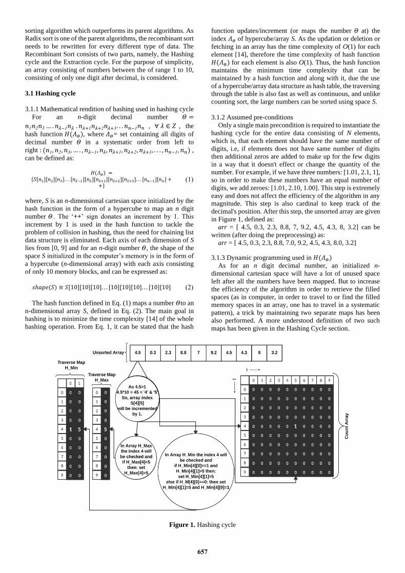
in Figure 1, defined as:
arr = [ 4.5, 0.3, 2.3, 8.8, 7, 9.2, 4.5, 4.3, 8, 3.2] can be
written (after doing the preprocessing) as:
arr = [ 4.5, 0.3, 2.3, 8.8, 7.0, 9.2, 4.5, 4.3, 8.0, 3.2]
3.1.3 Dynamic programming used in 𝐻(𝛬𝛩)
As for an n digit decimal number, an initialized n-
dimensional cartesian space will have a lot of unused space
left after all the numbers have been mapped. But to increase
the efficiency of the algorithm in order to retrieve the filled
spaces (as in computer, in order to travel to or find the filled
memory spaces in an array, one has to travel in a systematic
pattern), a trick by maintaining two separate maps has been
also performed. A more understood definition of two such
maps has been given in the Hashing Cycle section.
Figure 1. Hashing cycle
657

The steps of the hashing cycle are lucidly depicted in Figure
1 (the hashing function 𝐻(𝛬𝛩) defined above is used for each
element of the unsorted array arr). For sorting the type of data
considered in the example, a 2D array of dimension 10x10
called the Count array, where the values will be mapped is
considered, a traverse map H_Max of dimension 10x1 and a
traverse map H_Min of dimension 10x2 are also taken. The
two traverse maps are used to avoid unnecessary steps during
the extraction period. The algorithm for hashing cycle
designed for the example considered is as follows:
_________________________________________________
HASHING CYCLE ALGORITHM: The algorithm
presented below uses two function: First, the numeric to string
converter function, defined as: 𝐹𝑠𝑡𝑟𝑖𝑛𝑔()and second, the string
to numeric converter, defined as: 𝐹𝑁𝑢𝑚𝑒𝑟𝑖𝑐().
_________________________________________________
Recombinant-hashing(arr, size): //the unsorted array arr
S[10][10];
H_Max[10];
H_Min[10][2];
set digit_count_after_decimal ← 1
for i = 0 to size do
𝑡 = 𝐹𝑠𝑡𝑟𝑖𝑛𝑔(𝑎𝑟𝑟[𝑖] × (10𝑑𝑖𝑔𝑖𝑡_𝑐𝑜𝑢𝑛𝑡_𝑎𝑓𝑡𝑒𝑟_𝑑𝑒𝑐𝑖𝑚𝑎𝑙 ))
𝑆[𝐹𝑁𝑢𝑚𝑒𝑟𝑖𝑐(𝑡[0])][𝐹𝑁𝑢𝑚𝑒𝑟𝑖𝑐(𝑡[1])] ← 𝒊𝒏𝒄𝒓𝒆𝒎𝒆𝒏𝒕 𝑏𝑦 1
if( 𝐻_𝑀𝑎𝑥[𝐹𝑁𝑢𝑚𝑒𝑟𝑖𝑐(𝑡[0])] < 𝐹𝑁𝑢𝑚𝑒𝑟𝑖𝑐(𝑡[1])) then
set 𝐻_𝑀𝑎𝑥[𝐹𝑁𝑢𝑚𝑒𝑟𝑖𝑐(𝑡[0])] ← 𝐹𝑁𝑢𝑚𝑒𝑟𝑖𝑐(𝑡[1])
if (𝐻_𝑀𝑖𝑛[𝐹𝑁𝑢𝑚𝑒𝑟𝑖𝑐(𝑡[0])][0] == 0) then
set 𝐻_𝑀𝑖𝑛[𝐹𝑁𝑢𝑚𝑒𝑟𝑖𝑐(𝑡[0])][1] ←𝐹𝑁𝑢𝑚𝑒𝑟𝑖𝑐(𝑡[1])
set 𝐻_𝑀𝑖𝑛[𝐹𝑁𝑢𝑚𝑒𝑟𝑖𝑐(𝑡[0])][0] ← 1
else if (𝐻_𝑀𝑖𝑛[𝐹𝑁𝑢𝑚𝑒𝑟𝑖𝑐(𝑡[0])][0] ≠ 0 and
𝐻_𝑀𝑖𝑛[𝐹𝑁𝑢𝑚𝑒𝑟𝑖𝑐(𝑡[0])][1] > 𝐹𝑁𝑢𝑚𝑒𝑟𝑖𝑐(𝑡[1])) then
set 𝐻_𝑀𝑖𝑛[𝐹𝑁𝑢𝑚𝑒𝑟𝑖𝑐(𝑡[0])][1] ← 𝐹𝑁𝑢𝑚𝑒𝑟𝑖𝑐(𝑡[1])
end for( i )
end func
_________________________________________________
As depicted in Figure 1, the array arr (defined above) is fed
to the hashing cycle for sorting and the space S of 10x10 is
initialized along with a vector H_Max of shape 10 and a space
H_Min of shape 10x2. The further steps are as follows:
1. The first element of the array is ‘4.5’, so:
a. First, it will be multiplied by 101 (as count after
decimal is 1): 4.5×10 = 45
b. Second, the number 45 will be converted to string
using 𝐹𝑆𝑡𝑟𝑖𝑛𝑔(45) = t = ‘45’.
c. Third, we will increment the value in the memory
block at row t[0] = 4 and column t[1] = 5 (at array
index (4, 5)).
d. Fourth, in the traverse map H_Max, as H_Max
[t[0]] < t[1], then H_Max[t[0]] will be set as t[1].
e. Fifth, in traverse map H_Min, as H_Min [t[0]][0]
= = 0, then H_Min[t[0]][1] will be set as t[1] and
H_Min[𝐹𝑁𝑢𝑚𝑒𝑟𝑖𝑐(t[0])][0] will be set to 1.
f. Lastly, the complete process will continue for each
array element till we reach the end of the unsorted
array and the rest of the complete steps are given in
the example 1 in the supplementary section.
3.2 Extraction cycle
The end result of the hashing cycle is depicted in Figure 2.
For the extraction of sorted arrays from the count array, the
exaction cycle moves row by row, like done in raster scanning,
for example, the cycle will visit all indices of row 0 and then
all indices of row 1 and so on.
Figure 2. Extraction cycle
It is clear from Figure 2 that most of the memory spaces in
the count array are not filled and thus, traversing these unused
spaces will increase the time complexity of the algorithm. So,
in order to minimize the time complexity and prevent wasteful
traversal of these unused spaces, the traverse maps H_Min and
H_Max are used. In the Traverse map H_Min, each row stores
the lowest numeric value attained by the columns for that
particular row in the count array and in the Traverse map
H_Max, each row stores the highest numeric value attained by
the columns for that particular row in the count array, for
example, for row 4 in the count array the minimum column
reached is 3 and the maximum column reached is 5, so the
traverse map H_Min will store the value 3 and of H_Max will
store the value 5, for row 4 of the count array. The column 0
of the traverse map H_Min will store whether the map for that
particular row had been updated before or not. The algorithm
for extraction cycle is as follows:
_________________________________________________
EXTRACTION CYCLE ALGORITHM: The algorithm
presented below uses a function defined as:
Overwrite_arr(element, position, arr). This function
overwrites the element ‘element’ at position ‘position’ of array
‘arr’. The importance of pre-conditions, defined above, can be
seen in line 7. The 𝐹𝐹𝑙𝑜𝑎𝑡() function used below converts
strings to float numbers and numeric to string converter
function is also used and is defined as: 𝐹𝑠𝑡𝑟𝑖𝑛𝑔(). In line 7, the
‘+’ sign is used to represent string concatenation.
_________________________________________________
Recombinant-extraction(S, H_Min, H_Max,arr, size):
set overwrite_pos_at ← 0
for i = 0 to 9 do
for j = H_Min[i][1] to H_Max[i]+1 do
if(S[i][j]!=Empty) then
for z = 0 to S[i][j] do
Overwrite_arr(𝐹𝐹𝑙𝑜𝑎𝑡(𝐹𝑠𝑡𝑟𝑖𝑛𝑔(i)+'.'+
𝐹𝑠𝑡𝑟𝑖𝑛𝑔(j)), overwrite_pos_at, arr)
overwrite_pos_at ← increment by 1
if(overwrite_pos_at == size) then
return arr
end func
658
end for( z )
end for( j )
end for( i )
end func _________________________________________________
At the end of the extraction cycle, the parts of the count
array traversed are shown in Figure 2 and the sorted array
obtained is shown below. The time complexity of the example
taken in the prior section is found to be O(n+17). Sorted array
arr returned as:
[0.3, 2.3, 3.2, 4.3, 4.5, 4.5, 7.0, 8.0, 8.8, 9.2]
Why Does Extraction Cycle Work?
As it is known that in a computer’s memory, in order to
travel through an n-dimensional space one has to travel in a
systematic pattern, performed using for loops. This systematic
pattern traversal has a unique ability, whose advantage has
been taken during the extraction cycle. A similar pattern can
be observed when traversing a Binary Search Tree in an
inorder traversal fashion. By traversing inorderly, a sorted
form of the unsorted data used to build the binary search tree
can be obtained. Due to the unique hash function 𝐻(𝛬𝛩)used
to map an n-digit number 𝛩 to an n-dimensional cartesian
space, a unique sorted outcome observed when performing
inorder traversal in a binary search can also be observed when
using Extraction Cycle (proposed above) to traverse through
an n-dimensional cartesian space.
4. PROOF OF CORRECTNESS
Loop Invariant Induction [14] method has been used to
prove the correctness of the proposed algorithm. It has been
used to prove the correctness of both the Hashing Cycle and
the Extraction Cycle. The correctness is for the recombinant
sorting algorithm for n digit decimal numbers (the pseudo code
for which is given in Supplementary Section).
Notations: The unsorted array is denoted by arr[] and S is
used to denote the initialized n-dimensional space. The two
arrays used to lower the extraction cost of the algorithm are
denoted by H_Min and H_Max. It is assumed that arr[]
contains N elements and the precondition stated above has
been satisfied, and therefore, each element of arr[] has n digits.
It is also assumed that the decimal point is placed after
𝜆𝑡ℎ,∀ 𝜆 ∈ 𝑍, digit for each element and thus, λ digits lie before
the decimal and (n-λ) digits lie after decimal for each element.
4.1 Hashing cycle
The predominant objective of this function is to use 𝐻(𝛬𝛩)
so as to map all n elements of arr[] to an n-dimensional
cartesian space, which is in the form of an array in the
computer’s memory. So, for every element in arr[], there
exists a place in the n-dimensional space. Therefore, the loop
invariant 𝐼𝐻𝑎𝑠ℎ for iteration 𝑖𝑡ℎcan be defined as,
𝐼𝐻𝑎𝑠ℎ ≡ At iteration i, the initialized n-dimensional empty
cartesian space S should have ≤ 𝑖 points mapped in it by using
𝐻(𝛬𝛩). Also, the arrays H_Min and H_Max should have ≤ 2𝑖 and ≤ 𝑖 spaces mapped in it respectively.
Or
𝐼𝐻𝑎𝑠ℎ ≡ At iteration i, the cycle should successfully map all
elements in arr[0: i] using𝐻(𝛬𝛩), to an n-dimensional space
S, initialized prior to the starting of loop.
The three steps for Loop invariant proof are as follows:
(1) Initialization: Before the first iteration of the loop or
at i=0 in the cycle, the invariant 𝐼𝐻𝑎𝑠ℎ states that the initialized
n-dimensional empty cartesian space should have ≤ 0 points
mapped in it by using 𝐻(𝛬𝛩). Also, the arrays H_Min and
H_Max should have ≤ 2 ∗ 0 and ≤ 0 spaces mapped in it,
respectively. As 0 points have been mapped in space S at i=0,
therefore the space remains vacant. Also, 0 spaces in arrays
H_Min and H_Max have been mapped, therefore they also
remain unoccupied. As the space S and arrays H_Min and
H_Max were already set to be vacant, the invariant condition
stands corrected.
(2) Maintenance: Assume that the loop invariant stands
corrected at the start of iteration i=j in the cycle. Then it must
be that the initialized n-dimensional empty cartesian space S
should have ≤ 𝑗points mapped in it by using 𝐻(𝛬𝛩). Also, the
arrays H_Min and H_Max should have≤ 2 ∗ 𝑗 and ≤ 𝑗 spaces
mapped in it respectively. In the body of the loop at iteration j,
arr[j] is mapped to cartesian space S, and if the defined
condition holds True, then the required values are mapped in
arrays H_Min and H_Max. Thus, at the start of the iteration i
= j+1, the initialized n-dimensional empty cartesian space S
will have ≤ 𝑗 + 1points mapped in it by using 𝐻(𝛬𝛩). Also,
the arrays H_Min and H_Max will have ≤ 2 ∗ (𝑗 + 1) and ≤𝑗 + 1spaces mapped in it respectively, which needed to be
proved.
(3) Termination: When the for-loop terminates at i = N,
the initialized n-dimensional empty cartesian space S has ≤𝑁points mapped in it by using 𝐻(𝛬𝛩). Also, the arrays H_Min
and H_Max has ≤ 2 ∗ 𝑁 and ≤ 𝑁 spaces mapped in it
respectively. As arr[] has N elements, therefore all elements
have been mapped to space S, which is also the desired output.
As all three steps of the loop invariant hold true, therefore
the algorithm for the hash cycle is correct.
4.2 Extraction cycle
It is a known fact that a human can traverse an n-
dimensional space in either a linear or a nonlinear fashion, but
computers can only traverse such spaces in a linear fashion.
This linear traversal, as also mentioned before, yields an
advantage. For instance, in order to traverse through a 2-
dimensional space of size 10×10, a for or while-loop is needed,
and upon discerning those loops closely, one would notice that
they are intrinsically counting from 0 to 100 (and undeniably
counting is sorted). Thus, the extraction cycle traverses the n-
dimensional space in a fashion that it encounters the mapped
elements in a sorted manner, due to the intrinsic nature of loop
traversal. n+1 number of for-loops are required for traversing
an n-dimensional array, as well as for extracting the numbers
mapped. In order to define n+1 for-loops, n+1 number of
iterators will be needed, and can be defined as:
(𝑖1, 𝑖2, 𝑖3, . . . , 𝑖𝑛−1, 𝑖𝑛 , 𝑖𝑛+1). Another variable overwrite_at_pos
is defined to keep track of how many occupied spaces in S have
been detected and tells where to overwrite the original
unsorted array. The loop invariant IExtract for every ith iteration
can be defined as,
𝑰𝑬𝒙𝒕𝒓𝒂𝒄𝒕 ≡ At iteration overwrite_at_pos = j and iterators
𝑖1, 𝑖2, 𝑖3, . . . , 𝑖𝑛−1, 𝑖𝑛 𝑎𝑛𝑑 𝑖𝑛+1 having any value such that the
mentioned if-condition is satisfied, the element 𝐸𝑗+1 detected
659
at 𝑆[𝑖1][𝑖2][𝑖3]. . . [𝑖𝑛−1][𝑖𝑛+1] can be represented as:
𝐸1, 𝐸2, 𝐸3, . . . , 𝐸𝑗 ≤ 𝐸𝑗+1 ≤ 𝐸𝑗+2, 𝐸𝑗+3, 𝐸𝑗+4, . . . , 𝐸𝑁 (3)
And the overwritten sub-array arr[0:j] should be sorted or
the sub-array arr[j:N] should be unsorted or unchanged.
The three steps for Loop invariant proof are as follows:
(1) Initialization: Before the first iteration of the loop or
at overwrite_at_pos=j=0 and iterators
𝑖1, 𝑖2, 𝑖3, . . . , 𝑖𝑛−1, 𝑖𝑛 , 𝑖𝑛+1 having any value such that the
mentioned if-condition is satisfied, the element 𝐸1 detected at
𝑆[𝑖1][𝑖2][𝑖3]. . . [𝑖𝑛−1][𝑖𝑛+1] can be represented as:
𝐸1 ≤ 𝐸2, 𝐸3, 𝐸4, . . . , 𝐸𝑁 (4)
And the overwritten sub-array arr[0:0] should be sorted or
the sub-array arr[0:N] should be unsorted or unchanged. As
the size of the overwritten sub-array arr[0:0] is zero, or the
overwritten sub-array arr[0:0] is completely empty, therefore,
it is sorted. Also, as the sub-array arr[0:N] was already
unsorted or unchanged, the invariant condition stands
corrected.
(2) Maintenance: Assume that the loop invariant stands
corrected at the start of iteration overwrite_at_pos=j=z and
and iterators 𝑖1, 𝑖2, 𝑖3, . . . , 𝑖𝑛−1, 𝑖𝑛 , 𝑖𝑛+1 having any value such
that the mentioned if-condition is satisfied in the cycle. Then
it must be that the element 𝐸𝑧+1 detected at
𝑆[𝑖1][𝑖2][𝑖3]. . . [𝑖𝑛−1][𝑖𝑛+1]can be represented as:
𝐸1, 𝐸2, 𝐸3, . . . , 𝐸𝑧−1 ≤ 𝐸𝑧+1 ≤ 𝐸𝑧+2, 𝐸𝑧+3, 𝐸𝑧+4, . . . , 𝐸𝑁 (5)
And the overwritten sub-array arr[0:z] should be sorted or
the sub-array arr[z:N] should be unsorted or unchanged. In the
body of the loop at iteration overwrite_at_pos=j=z, the
extracted element is overwritten at index z of unsorted array
arr[], leaving sub-array arr[0:z] sorted or sub-array arr[z:N]
unsorted or unchanged. Thus, at the start of iteration
overwrite_at_pos=j=z+1 and iterators
𝑖1, 𝑖2, 𝑖3, . . . , 𝑖𝑛−1, 𝑖𝑛 , 𝑖𝑛+1 having any value such that the
mentioned if-condition is satisfied in the cycle, the element
𝐸𝑧+2 detected at 𝑆[𝑖1][𝑖2][𝑖3]. . . [𝑖𝑛−1][𝑖𝑛+1]will be represented
as:
𝐸1, 𝐸2, 𝐸3, . . . , 𝐸𝑧+1 ≤ 𝐸𝑧+2 ≤ 𝐸𝑧+3, 𝐸𝑧+4, 𝐸𝑧+5, . . . , 𝐸𝑁 (6)
And the overwritten sub-array arr[0:z+1] will be sorted or
the sub-array arr[z+1:N] will be unsorted or unchanged,
which needed to be proved.
(3) Termination: When the for-loop terminates at
overwrite_at_pos=j=N and iterators
𝑖1, 𝑖2, 𝑖3, . . . , 𝑖𝑛−1, 𝑖𝑛 , 𝑖𝑛+1 having any value such that the
mentioned if-condition is satisfied in the cycle, then the
element 𝐸𝑁+1 detected at 𝑆[𝑖1][𝑖2][𝑖3]. . . [𝑖𝑛−1][𝑖𝑛+1] is
represented as:
𝐸1, 𝐸2, 𝐸3, 𝐸4, . . . , 𝐸𝑁 ≤ 𝐸𝑁+1 (7)
As EN+1 does not exist, therefore, all N elements have been
detected and overwritten. Also, the overwritten sub-array
arr[0:N] will be sorted or the sub-array arr[N:N] will have
size zero or contain zero elements, which is also the desired
output.
As all three steps of the loop invariant hold true, therefore
the algorithm for the extraction cycle is correct. Also, as both
the hashing cycle and extraction cycle are correct, it renders
the proposed Recombinant Sort algorithm correct. The
correctness of the algorithm can also be verified from the
example 1 described in the supplementary section.
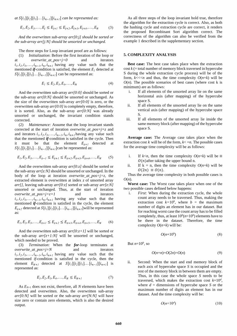
5. COMPLEXITY ANALYSIS
Best case: The best case takes place when the extraction
cost k (= total number of memory block traversed in hypercube
S during the whole extraction cycle process) will be of the
form, k<<<n and thus, the time complexity O(n+k) will be
O(n). The possible scenarios of best cases (where cost k is
minimum) are as follows:
i. If all elements of the unsorted array lie on the same
horizontal axis (after mapping) of the hypercube
space S.
ii. If all elements of the unsorted array lie on the same
vertical axis (after mapping) of the hypercube space
S.
iii. If all elements of the unsorted array lie inside the
same memory block (after mapping) of the hypercube
space S.
Average case: The Average case takes place when the
extraction cost 𝑘 will be of the form, k< =n. The possible cases
for the average time complexity will be as follows:
i. If k<n, then the time complexity O(n+k) will be ≡𝑂(𝑛)after taking the upper bound n.
ii. If k = n, then the time complexity O(n+k) will be
𝑂(2𝑛) ≡ 𝑂(𝑛).
Thus the average time complexity in both possible cases is
O(n).
Worst case: The Worst case takes place when one of the
two possible cases defined below happens:
i. First: When during the extraction cycle, the whole
count array needs to be traversed. Thus, making the
extraction cost k=10b, where b = the maximum
number of digits an element has in our dataset. But
for reaching worst case the count array has to be filled
completely, thus, at least 10b(n=10b) elements have to
be there in the dataset. Therefore, the time
complexity O(n+k) will be:
O(n+10b) (8)
But n=10b, so
O(n+n)=O(2n)=O(n) (9)
ii. Second: When the start and end memory block of
each axis of hypercube space S is occupied and the
rest of the memory block in between them are empty.
Thus, in this case the whole space S needs to be
traversed, which makes the extraction cost k=10d,
where d = dimensions of hypercube space S or the
maximum number of digits an element has in our
dataset. And the time complexity will be:
O(n+10d) (10)
660

But for this case to be valid, the total number of elements to
be sorted should be =10d. Thus, it can be stated that n=10d and
the Eq. (10) can be written as:
𝑂(10𝑑 +10𝑑) (11)
𝑂 (10𝑑 (1 + 10(𝑑−1)
𝑑)) (12)
As n =10d,
𝑂 (𝑛 (1 + 10(𝑑−1)
𝑑)) (13)
Which can be further simplified as,
𝑂(𝑛𝐶) (14)
where, C =(1 +10(𝑑−1)
𝑑).
Figure 3. Relationship between constant C, n, 𝑛2 and d
On the basis of experiment, whose results are shown in
Figure 3, (by putting different values of d) it was observed that:
𝐶 < 𝑛2 (15)
Thus, from Eq. (15) we can state that C is a constant that
will never make the time complexity nonlinear and the
complexity given in Eq. (14) can be written as O(n).
Thus, the time complexity will always be linear.
6. RESULTS AND DISCUSSIONS
Table 1 shows the time taken by the system to execute
recombinant sort using Python on Mac OS. The sorting
method is executed in Python, C++ and Java language on Mac
OS, Windows OS and Linux OS. The system had 3.1 GHz
Intel Core i5 processor and 8 GB 2133 MHz LPDDR3 RAM.
The testing data is generated from a random generator function
available in python’s numpy library. The number of elements
taken for the execution of recombinant sort ranges from 10 to
10000, increasing in powers of 10. Time is calculated for five
major cases, namely, for data between the range of 1 to 10
having no digits after the decimal, having a single digit after
the decimal and having two digits after the decimal, and for
data between the range of 1 to 100 having no digits after the
decimal and having a single digit after the decimal. The time
taken for a specific number of elements for all the cases are of
comparable order, as can be seen from Table 1. The results
obtained by running the algorithm in different languages on
different operating systems platforms are shown in tabular
format (Tables 4-11), along with their graphical representation
(Figure 5), are given in the supplementary section. These
languages (Python, C++ and Java) and operating systems
(Window, Mac and Linux) have been chosen specifically as
they are very widely used.
Figure 4 depicts the results obtained in Table 1 in a
graphical manner. The graph shows the time taken to execute
recombinant sort (in milliseconds) for all the five enlisted
cases. The graph depicts linear characteristics of the proposed
sorting algorithm and it can also be concluded from the graph
that the count_after_decimal variable hardly affects the time
complexity. These same observations can also be made while
observing the graphs (for Python, C++ and Java languages and
Mac OS, Windows OS and Linux OS) given in the
supplementary section.
Table 2 gives a complete comparison between various
existing and known sorting algorithms and the proposed
Recombinant sort technique on the basis of various cardinal
factors like best case time complexity, average case time
complexity, worst case time complexity, stability, in-place or
out-of-place sorting and the ability to process strings and
floating point numbers.
Figure 4. Relationship between the number of elements and
the time taken by Recombinant Sort to sort elements using
Python on Mac OS
Table 1. The time taken (in sec) by the system to execute recombinant sort using python on Mac OS
No. of elements TFD (1,10) & cd=0 TFD (1,10) & cd=1 TFD (1,10) & cd=2 TFD (1,100) & cd=0 TFD (1,100) & cd=1)
10 0.00066 0.00078 0.00091 0.00079 0.00091
100 0.00581 0.00649 0.00792 0.00641 0.007.91
1000 0.5790 0.06124 0.06889 0.06112 0.06821
10000 0.57410 0.60279 0.61084 0.59412 0.61038 Note: The expression TFD(a,b) & cd = c stands for: Time For sorting Data ranging between a to b, and count after decimal = c respectively.
661

Table 2. Comparison with other sorting algorithms
Sorting algorithm Best TC Average TC Worst TC stable sort PD PS IP
Bubble sort [15] O(n)
(waas) O(n2) O(n2) Yes Yes No Yes
Selection Sort [16] O(n2) O(n2) O(n2) No Yes No Yes
Insertion Sort [17] O(n2) (waas) O(n2) O(n2) Yes Yes No Yes
Merge Sort [18] O(nlogn) O(nlogn) O(nlogn) Yes Yes No No
Quick Sort [19] O(nlogn) O(nlogn) O(n2) No Yes No Yes
Bucket Sort [9] O(n+c) O(n+c) O(n2) Yes Yes No No
Radix Sort [12] O(kn)
(k∈Z) O(kn) (k∈Z) O(kn) (k∈Z) Yes No Yes No
Heap Sort [20] O(nlogn) O(nlogn) O(nlogn) No Yes No Yes
Tim Sort [21] O(n)
(waas) O(nlogn) O(nlogn) Yes Yes No No
Shell Sort [22] O(n)
(waas) O(n2) O(n2) No Yes No Yes
Counting Sort [11] O(n) O(n+c) O(n2) Yes No No No
Recombinant Sort O(n) O(n) O(n) No Yes Yes No Note: waas stands for: When array is already sorted; TC stands for Time Complexity; PD: Can Sort or Process Decimals; PS: Can Sort or Process Strings; IP:
Inplace Sort; Z: integer.
Table 3. Dimensions of elements required for sorting different types of data
S.
No.
Type of
Data
Dimensions of
Count Array
Dimensions of
Traverse Map H_Min
Dimensions of
Traverse Map H_Max
1. D(1,10) & cd = 0 10 2 1
2. D(1,10) & cd = 1 10x10 10x2 10x1
3. D(1,10) & cd = 2 10x10x10 10x22 10x11
4. D(1,100) & cd = 0 10x10 10x2 10x1
5. D(1,100) & cd = 1 10x10x10 10x22 10x11 Note: The expression D(a,b) & cd = c stands for: Data ranging between a to b, and count after decimal = c respectively.
From Table 2, it is observed that merge sort and heap sort
have the consistent time complexity of O(nlogn) for the best,
average and worst case scenarios, but none of these sorting
methods can be used to sort elements of string data type.
Quicksort also has O(nlogn) time complexity for the best and
average cases, but resorts to being O(n2) for the worst case, i.e.
when the array is already sorted in any order or when the array
contains all identical elements. Tim sort has the time
complexity O(nlogn) for the worst and average cases and O(n)
for the best case (given that the array is already sorted). Unlike
the sorting algorithms listed above, the proposed recombinant
sort has consistent performance of O(n) for the best case,
average case and worst case scenarios. In addition to this,
recombinant sort can also be used to sort elements of string
data type and floating type. Therefore, it can be observed that
the proposed recombinant sort performs best among all the
listed sorting algorithms.
Table 3 specifies the dimensions of the elements
constituting the recombinant sort, that is, the count array, and
the H_Min and H_Max traverse maps, for sorting data
elements that belong to the data specified in the five cases
enlisted previously.
This table depicts a pattern that can be followed to deal with
different types of data (not mentioned in the table) using
Recombinant Sort.
7. CONCLUSION AND FUTURE WORK
The proposed Recombinant Sort is a dynamic sorting
technique which can be modified as per the needs of the user
and is designed to achieve utmost efficiency for sorting data
of varied types and ranges. The time complexity of the
proposed Recombinant Sort is estimated to be O(n+k) for best,
average and worst cases. The k in O(n+k) will become n in the
worse case scenario, but in no circumstance will n’s order
approaches two, i.e, k will never approach n2, thus, the
complexity will never be O(n2). The extraction cost 𝑘, will
always be very less than or equal to 𝑛, thus, the final time
complexity will always be O(n). Also, the extraction cost 𝑘 of
the proposed Recombinant Sort came out to be much smaller
than the extraction cost of any other linear sorting algorithms.
The graph plotted between the number of elements and the
time taken by recombinant sort to sort those elements depicts
a linear characteristic.
All major highlighted demerits of the parent algorithms of
the Recombinant Sort, i.e., counting sort, radix sort and bucket
sort, are surmounted by Recombinant Sort. Recombinant Sort
can process strings as well as numbers, and can also process
both floating point and integer type numbers together. Though,
with the increase in the number of digits in elements to be
sorted, the dimensions of the count array will increase, and the
complexity of the working of the algorithm will also increase.
But an important thing to note here is that, in the physical
world, we don’t usually deal with numbers containing more
than 10 digits, be it, marks obtained or the net salaries. By
testing the algorithm on all possible types of data, it has been
empirically proved that the proposed algorithm is correct,
complete and terminates at the end. Thus, Recombinant Sort is
a viable option from the user’s perspective. In order to accredit
fair competition, an open source library named Recombinant
Sort has been released on github.
In the future, the proposed Recombinant Sort can be
enhanced by sorting integer, string and floating type elements
without rewriting the entire program for these specific needs.
Another noteworthy addition to the current proposed
algorithm can be made post-availability of advanced literature
on N-dimensional space or hypercubes.
662

REFERENCES
[1] Sorting. Definition of Sorting. En.wikipedia.org.
https://en.wikipedia.org/wiki/Sorting, accessed on May
20, 2020.
[2] Aung, H.H. (2019). Analysis and comparative of sorting
algorithms. International Journal of Trend in Scientific
Research and Development (IJTSRD), 3(5): 1049-1053.
https://doi.org/10.31142/ijtsrd26575
[3] Comparison Sort Definition. En.wikipedia.org.
https://en.wikipedia.org/wiki/Comparison_sort,
accessed on May 20, 2020.
[4] In-place Sorting Technique. 2020. En.wikipedia.org.
https://en.wikipedia.org/wiki/In-place_algorithm,
accessed on May 20, 2020.
[5] Verma, A.K., Kumar, P. (2013). List sort: A new
approach for sorting list to reduce execution time. arXiv
preprint arXiv:1310.7890.
[6] Stable Sorts Definition. En.wikipedia.org.
https://en.wikipedia.org/wiki/Category:Stable_sorts,
accessed on May 22, 2020.
[7] Singh, M., Garg, D. (2009). Choosing best hashing
strategies and hash functions. In proceedings of 2009
IEEE International Advance Computing Conference,
Patiala, pp. 50-55.
https://doi.org/10.1109/IADCC.2009.4808979
[8] Mohammad, S., Kumar, A.R. (2019). SA sorting: A
novel sorting technique for large-scale data. Journal of
Computer Networks and Communications, 2019:
3027578. https://doi.org/10.1155/2019/3027578
[9] Bucket Sort Definition. En.wikipedia.org.
https://en.wikipedia.org/wiki/Bucket_sort, accessed on
May 22, 2020.
[10] Abdulla, P.A. (2009). Counting Sort.
[11] Counting Sort Definition. En.wikipedia.org.
https://en.wikipedia.org/wiki/Counting_sort, accessed
on May 23, 2020.
[12] Radix Sort Definition. En.wikipedia.org.
https://en.wikipedia.org/wiki/Radix_sort, accessed on
May 23, 2020.
[13] Abdulla, P.A. (2011). Radix Sort. Encyclopedia of
Parallel Computing.
[14] Cormen, T.H., Leiserson, C.E., Rivest, R.L., Stein, C.
(2009). Introduction to Algorithms. MIT press.
[15] Astrachan, O.L. (2003). Bubble sort: An archaeological
algorithmic analysis. SIGCSE, 35(1).
https://doi.org/10.1145/792548.611918
[16] Chand, S., Chaudhary, T., Parveen, R. (2011). Upgraded
selection sort. International Journal on Computer Science
and Engineering, 3(4): 1633-1637.
[17] Kowalk, W.P. (2011). Insertion Sort. In: Vöcking B. et
al. (eds) Algorithms Unplugged. Springer, Berlin,
Heidelberg. https://doi.org/10.1007/978-3-642-15328-
0_2
[18] Wang, B. (2008). Merge Sort. (2008).
[19] Hennequin, P. (1989). Combinatorial analysis of
quicksort algorithm. RAIRO-Theoretical Informatics
and Applications, 23(3): 317-333.
https://doi.org/10.1051/ita/1989230303171
[20] Schaffer, R., Sedgewick, R. (1993). The analysis of
heapsort. Journal of Algorithms, 15(1): 76-100.
https://doi.org/10.1006/jagm.1993.1031
[21] Auger, N., Jugé, V., Nicaud, C., Pivoteau, C. Analysis of
TimSort Algorithm. http://igm.univ-
mlv.fr/~juge/slides/poster/ligm-2019.pdf, accessed on
Jun. 2, 2020.
[22] Sedgewick, R. (1996). Analysis of Shellsort and related
algorithms. In: Diaz J., Serna M. (eds) Algorithms - ESA
'96. ESA 1996. Lecture Notes in Computer Science, vol
1136. Springer, Berlin, Heidelberg.
https://doi.org/10.1007/3-540-61680-2_42
SUPPLEMENTARY SECTION
________________________________________________________________________________________________________
HASHING CYCLE ALGORITHM FOR n DIGIT NUMBER: The algorithm presented below uses two function: First, the
numeric to string converter function, defined as: 𝐹𝑠𝑡𝑟𝑖𝑛𝑔()and second, the string to numeric converter, defined as: 𝐹𝑁𝑢𝑚𝑒𝑟𝑖𝑐().
NOTE: In day to day life we usually deal with 4-5 digit numbers.
________________________________________________________________________________________________________
Recombinant-hashing(arr , size,𝜆) // the unsorted array arr
1. S[10][10][10]..[10][10]; // n dimensional count array S is initialized
2. H_Max[10][10][10]..[10][10]; // (n-1) dimensional traverse map H_Max is
initialized
3. H_Min[10][222...222]; // traverse map H_Min is initialized. (n-1) 2’s are
there
4. set digit_count_after_decimal← 𝜆
5. for i = 0 to size do
6. 𝑡 = 𝐹𝑠𝑡𝑟𝑖𝑛𝑔(𝑎𝑟𝑟[𝑖] × (10𝑐𝑜𝑢𝑛𝑡_𝑎𝑓𝑡𝑒𝑟_𝑑𝑒𝑐𝑖𝑚𝑎𝑙 )) //converts number
to string
7. 𝑆[𝐹𝑁𝑢𝑚𝑒𝑟𝑖𝑐(𝑡[0])][𝐹𝑁𝑢𝑚𝑒𝑟𝑖𝑐(𝑡[1])]. . . [𝐹𝑁𝑢𝑚𝑒𝑟𝑖𝑐(𝑡[𝑛 − 1])] ← 𝒊𝒏𝒄𝒓𝒆𝒎𝒆𝒏𝒕 𝑏𝑦 1
8. if( 𝐻_𝑀𝑎𝑥[𝐹𝑁𝑢𝑚𝑒𝑟𝑖𝑐(𝑡[0])][0] < 𝐹𝑁𝑢𝑚𝑒𝑟𝑖𝑐(𝑡[1])) then // checking H_Max
9. set 𝐻_𝑀𝑎𝑥[𝐹𝑁𝑢𝑚𝑒𝑟𝑖𝑐(𝑡[0])][0] ← 𝐹𝑁𝑢𝑚𝑒𝑟𝑖𝑐(𝑡[1])
10. if (𝐻_𝑀𝑖𝑛[𝐹𝑁𝑢𝑚𝑒𝑟𝑖𝑐(𝑡[0])][0] == 0) then // if H_Min traverse map had been updated before
11. set 𝐻_𝑀𝑖𝑛[𝐹𝑁𝑢𝑚𝑒𝑟𝑖𝑐(𝑡[0])][1] ← 𝐹𝑁𝑢𝑚𝑒𝑟𝑖𝑐(𝑡[1])
12. set 𝐻_𝑀𝑖𝑛[𝐹𝑁𝑢𝑚𝑒𝑟𝑖𝑐(𝑡[0])][0] ← 1 // marking that the H_Min is updated
13. else if (𝐻_𝑀𝑖𝑛[𝐹𝑁𝑢𝑚𝑒𝑟𝑖𝑐(𝑡[0])][0] ≠ 0 and
𝐻_𝑀𝑖𝑛[𝐹𝑁𝑢𝑚𝑒𝑟𝑖𝑐(𝑡[0])][1] > 𝐹𝑁𝑢𝑚𝑒𝑟𝑖𝑐(𝑡[1])) then
14. set 𝐻_𝑀𝑖𝑛[𝐹𝑁𝑢𝑚𝑒𝑟𝑖𝑐(𝑡[0])][1] ← 𝐹𝑁𝑢𝑚𝑒𝑟𝑖𝑐(𝑡[1])
15. .
663
16. .
17. .
18. if( 𝐻_𝑀𝑎𝑥[𝐹𝑁𝑢𝑚𝑒𝑟𝑖𝑐(𝑡[0])][222. .221] < 𝐹𝑁𝑢𝑚𝑒𝑟𝑖𝑐(𝑡[𝑛 − 1])) then // checking H_Max
19. set 𝐻_𝑀𝑎𝑥[𝐹𝑁𝑢𝑚𝑒𝑟𝑖𝑐(𝑡[0])][10][10]. . . [10][10] ← 𝐹𝑁𝑢𝑚𝑒𝑟𝑖𝑐(𝑡[𝑛 − 1])
20. if (𝐻_𝑀𝑖𝑛[𝐹𝑁𝑢𝑚𝑒𝑟𝑖𝑐(𝑡[𝑛 − 1])][222. .220] == 0) then // if H_Min traverse map had been updated before
21. set 𝐻_𝑀𝑖𝑛[𝐹𝑁𝑢𝑚𝑒𝑟𝑖𝑐(𝑡[𝑛 − 1])][222. .221] ← 𝐹𝑁𝑢𝑚𝑒𝑟𝑖𝑐(𝑡[𝑛 − 1])
22. set 𝐻_𝑀𝑖𝑛[𝐹𝑁𝑢𝑚𝑒𝑟𝑖𝑐(𝑡[𝑛 − 1])][222. .220] ← 1 // marking that the H_Mi is updated
23. else if (𝐻_𝑀𝑖𝑛[𝐹𝑁𝑢𝑚𝑒𝑟𝑖𝑐(𝑡[𝑛 − 1])][222. .221] ≠ 0 and
𝐻_𝑀𝑖𝑛[𝐹𝑁𝑢𝑚𝑒𝑟𝑖𝑐(𝑡[𝑛 − 2])][222. . .221] > 𝐹𝑁𝑢𝑚𝑒𝑟𝑖𝑐(𝑡[𝑛 − 1])) then
24. set 𝐻_𝑀𝑖𝑛[𝐹𝑁𝑢𝑚𝑒𝑟𝑖𝑐(𝑡[𝑛 − 2])][222. .221] ← 𝐹𝑁𝑢𝑚𝑒𝑟𝑖𝑐(𝑡[𝑛 − 1])
25. end for( j )
26. end func
________________________________________________________________________________________________________
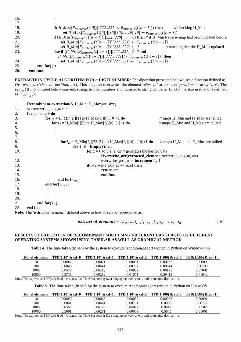
EXTRACTION CYCLE ALGORITHM FOR n DIGIT NUMBER: The algorithm presented below uses a function defined as:
Overwrite_arr(element, position, arr). This function overwrites the element ‘element’ at position ‘position’ of array ‘arr’. The
𝐹𝐹𝑙𝑜𝑎𝑡()function used below converts strings to float numbers and numeric to string converter function is also used and is defined
as: 𝐹𝑠𝑡𝑟𝑖𝑛𝑔().
________________________________________________________________________________________________________
Recombinant-extraction(S, H_Min, H_Max,arr, size)
1. set overwrite_pos_at ← 0
2. for 𝑖1 = 0 to 9 do
3. for 𝑖2 = H_Min[𝑖1][1] to H_Max[𝑖1][0]..[0]+1 do // maps H_Min and H_Max are tallied
4. for 𝑖3 = H_Min[i][2] to H_Max[𝑖1][0]..[1]+1 do // maps H_Min and H_Max are tallied
5. .
6. .
7. .
8. for 𝑖𝑛 = H_Min[𝑖1][22..21] to H_Max[𝑖1][10]..[10]+1 do // maps H_Min and H_Max are tallied
9. if(S[i][j]!=Empty) then
10. for z = 0 to S[i][j] do // generates the hashed data
11. Overwrite_arr(extracted_element, overwrite_pos_at, arr)
12. overwrite_pos_at ← increment by 1
13. if(overwrite_pos_at == size) then
14. return arr
15. end func
16. end for( 𝑖1𝑛 )
17. end for( 𝑖𝑛−1 )
18. .
19. .
20. .
21. end for( 𝑖1 )
22. end func
Note: The ‘extracted_element’ defined above in line 11 can be represented as:
𝒆𝒙𝒕𝒓𝒂𝒄𝒕𝒆𝒅_𝒆𝒍𝒆𝒎𝒆𝒏𝒕 = 𝑖1𝑖2𝑖3 … . 𝑖𝜆−1𝑖𝜆 . 𝑖𝜆+1𝑖𝜆+2𝑖𝜆+3. . . 𝑖𝑛−1𝑖𝑛 (16)
RESULTS OF EXECUTION OF RECOMBINANT SORT USING DIFFERENT LANGUAGES ON DIFFERENT
OPERATING SYSTEMS SHOWN USING TABULAR AS WELL AS GRAPHICAL METHOD
Table 4. The time taken (in sec) by the system to execute recombinant sort written in Python on Windows OS
No. of elements TFD(1,10) & cd=0 TFD(1,10) & cd=1 TFD(1,10) & cd=2 TFD(1,100) & cd=0 TFD(1,100) & cd=1)
10 0.00062 0.00071 0.00091 0.00085 0.0009
100 0.0049 0.00641 0.00797 0.00644 0.00783
1000 0.0572 0.06119 0.06882 0.06123 0.07001
10000 0.5738 0.60282 0.61071 0.59415 0.61042 Note: The expression TFD(a,b) & cd = c stands for: Time For sorting Data ranging between a to b, and count after decimal = c.
Table 5. The time taken (in sec) by the system to execute recombinant sort written in Python on Linux OS
No. of elements TFD(1,10) & cd=0 TFD(1,10) & cd=1 TFD(1,10) & cd=2 TFD(1,100) & cd=0 TFD(1,100) & cd=1)
10 0.00052 0.00063 0.00089 0.00083 0.00094
100 0.0041 0.00641 0.00791 0.0065 0.00777
1000 0.0569 0.06123 0.06872 0.0612 0.0702
10000 0.5681 0.60281 0.60039 0.5835 0.61061 Note: The expression TFD(a,b) & cd = c stands for: Time For sorting Data ranging between a to b, and count after decimal = c.
664

Table 6. The time taken (in sec) by the system to execute recombinant sort written in Java on Windows OS
No. of elements TFD (1,10) & cd=0 TFD (1,10) & cd=1 TFD (1,10) & cd=2 TFD (1,100) & cd=0 TFD (1,100) & cd=1)
10 0.00059 0.00069 0.00089 0.00085 0.00092
100 0.0044 0.00641 0.00791 0.00644 0.00782
1000 0.0572 0.06127 0.06822 0.06123 0.0701
10000 0.5682 0.60281 0.61066 0.57354 0.61039 Note: The expression TFD(a,b) & cd = c stands for: Time For sorting Data ranging between a to b, and count after decimal = c.
Table 7. The time taken (in sec) by the system to execute recombinant sort written in Java on Mac OS
No. of elements TFD (1,10) & cd=0 TFD (1,10) & cd=1 TFD (1,10) & cd=2 TFD (1,100) & cd=0 TFD (1,100) & cd=1)
10 0.00059 0.00071 0.00091 0.00085 0.00091
100 0.0046 0.00644 0.00792 0.00644 0.00785
1000 0.0574 0.06122 0.06885 0.06123 0.07011
10000 0.5732 0.60285 0.61069 0.59415 0.61039 Note: The expression TFD(a,b) & cd = c stands for: Time For sorting Data ranging between a to b, and count after decimal = c.
Table 8. The time taken (in sec) by the system to execute recombinant sort written in Java on Linux OS
No. of elements TFD (1,10) & cd=0 TFD (1,10) & cd=1 TFD (1,10) & cd=2 TFD (1,100) & cd=0 TFD (1,100) & cd=1)
10 0.00055 0.0007 0.00089 0.00081 0.00093
100 0.0047 0.00642 0.00791 0.00642 0.00783
1000 0.0569 0.06122 0.06123 0.06885 0.07013
10000 0.573 0.61068 0.60285 0.59339 0.6104 Note: The expression TFD(a,b) & cd = c stands for: Time For sorting Data ranging between a to b, and count after decimal = c.
Table 9. The time taken (in sec) by the system to execute recombinant sort written in C++ on Windows OS
No. of elements TFD (1,10) & cd=0 TFD (1,10) & cd=1 TFD (1,10) & cd=2 TFD (1,100) & cd=0 TFD (1,100) & cd=1)
10 0.00058 0.00071 0.00091 0.00083 0.00091
100 0.0045 0.00644 0.00792 0.00641 0.00782
1000 0.0575 0.06122 0.06885 0.06125 0.07021
10000 0.5731 0.59415 0.61069 0.60115 0.6104 Note: The expression TFD(a,b) & cd = c stands for: Time For sorting Data ranging between a to b, and count after decimal = c.
Table 10. The time taken (in sec) by the system to execute recombinant sort written in C++ on Mac OS
No. of elements TFD (1,10) & cd=0 TFD (1,10) & cd=1 TFD (1,10) & cd=2 TFD (1,100) & cd=0 TFD (1,100) & cd=1)
10 0.0005 0.00065 0.0009 0.00085 0.00094
100 0.0044 0.00641 0.00791 0.00644 0.00782
1000 0.0572 0.06127 0.06882 0.06123 0.0701
10000 0.5682 0.5682 0.61039 0.5835 0.61066 Note: The expression TFD(a,b) & cd = c stands for: Time For sorting Data ranging between a to b, and count after decimal = c.
Table 11. The time taken (in sec) by the system to execute recombinant sort written in C++ on Linux OS
No. of elements TFD (1,10) & cd=0 TFD (1,10) & cd=1 TFD (1,10) & cd=2 TFD (1,100) & cd=0 TFD (1,100) & cd=1)
10 0.00049 0.00061 0.00084 0.0008 0.00091
100 0.0036 0.0064 0.0079 0.0065 0.0077
1000 0.057 0.0612 0.0687 0.0612 0.0702
10000 0.5679 0.6028 0.6003 0.5835 0.6106 Note: The expression TFD(a,b) & cd = c stands for: Time For sorting Data ranging between a to b, and count after decimal = c.
665

Figure 5. Graphs A-H represent the linear characteristics depicted by tables 4-11 respectively
EXAMPLE 1
As depicted in Figure 1, the array arr (defined above) is fed
to the hashing cycle for sorting and the space S of 10x10 is
initialized along with a vector H_Max of shape 10 and a space
H_Min of shape 10x2. The further steps are as follows:
1. The first element of the array is ‘4.5’, so:
a. First, it will be multiplied by 101 (as count after
decimal is 1): 4.5×10 = 45
b. Second, the number 45 will be converted to string
using 𝐹𝑆𝑡𝑟𝑖𝑛𝑔(45) = t = ‘45’.
c. Third, we will increment the value in the memory
block at row t[0] = 4 and column t[1] = 5 (at array
index ( 4 , 5 ) ).
d. Fourth, in the traverse map H_Max, as H_Max
[ 𝐹𝑁𝑢𝑚𝑒𝑟𝑖𝑐 (t[0])] < 𝐹𝑁𝑢𝑚𝑒𝑟𝑖𝑐 (t[1]), then
H_Max[ 𝐹𝑁𝑢𝑚𝑒𝑟𝑖𝑐 (t[0])] will be set as
𝐹𝑁𝑢𝑚𝑒𝑟𝑖𝑐(t[1]).
e. Fifth, in traverse map H_Min, as H_Min
[ 𝐹𝑁𝑢𝑚𝑒𝑟𝑖𝑐 (t[0])][0] = = 0, then
H_Min[ 𝐹𝑁𝑢𝑚𝑒𝑟𝑖𝑐 (t[0])][1] will be set as
𝐹𝑁𝑢𝑚𝑒𝑟𝑖𝑐(t[1]) and H_Min[𝐹𝑁𝑢𝑚𝑒𝑟𝑖𝑐( t[0] )][0] will
be set to 1.
2. The first element of the array is ‘0.3’, so:
a. First, it will be multiplied by 101 (as count after
decimal is 1): 0.3×10 = 03
b. Second, the number 03 will be converted to string
using 𝐹𝑆𝑡𝑟𝑖𝑛𝑔(03) = t = ‘03’.
666
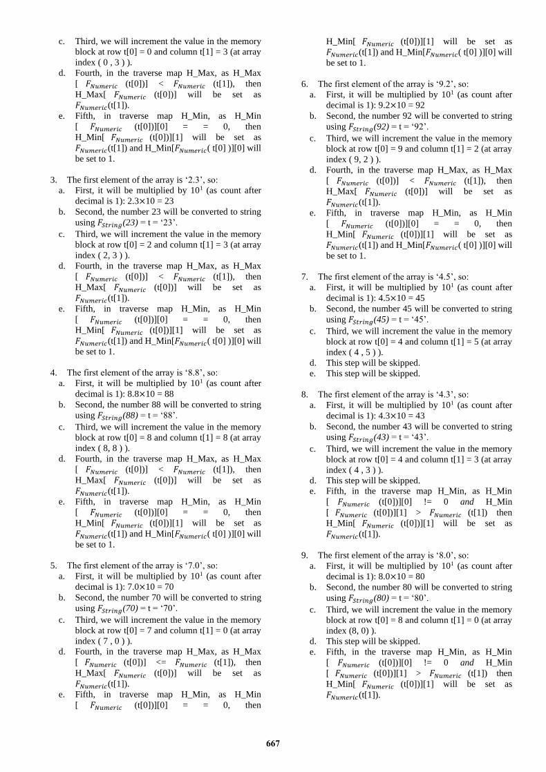
c. Third, we will increment the value in the memory
block at row t[0] = 0 and column t[1] = 3 (at array
index ( 0 , 3 ) ).
d. Fourth, in the traverse map H_Max, as H_Max
[ 𝐹𝑁𝑢𝑚𝑒𝑟𝑖𝑐 (t[0])] < 𝐹𝑁𝑢𝑚𝑒𝑟𝑖𝑐 (t[1]), then
H_Max[ 𝐹𝑁𝑢𝑚𝑒𝑟𝑖𝑐 (t[0])] will be set as
𝐹𝑁𝑢𝑚𝑒𝑟𝑖𝑐(t[1]).
e. Fifth, in traverse map H_Min, as H_Min
[ 𝐹𝑁𝑢𝑚𝑒𝑟𝑖𝑐 (t[0])][0] = = 0, then
H_Min[ 𝐹𝑁𝑢𝑚𝑒𝑟𝑖𝑐 (t[0])][1] will be set as
𝐹𝑁𝑢𝑚𝑒𝑟𝑖𝑐(t[1]) and H_Min[𝐹𝑁𝑢𝑚𝑒𝑟𝑖𝑐( t[0] )][0] will
be set to 1.
3. The first element of the array is ‘2.3’, so:
a. First, it will be multiplied by 101 (as count after
decimal is 1): 2.3×10 = 23
b. Second, the number 23 will be converted to string
using 𝐹𝑆𝑡𝑟𝑖𝑛𝑔(23) = t = ‘23’.
c. Third, we will increment the value in the memory
block at row t[0] = 2 and column t[1] = 3 (at array
index ( 2, 3 ) ).
d. Fourth, in the traverse map H_Max, as H_Max
[ 𝐹𝑁𝑢𝑚𝑒𝑟𝑖𝑐 (t[0])] < 𝐹𝑁𝑢𝑚𝑒𝑟𝑖𝑐 (t[1]), then
H_Max[ 𝐹𝑁𝑢𝑚𝑒𝑟𝑖𝑐 (t[0])] will be set as
𝐹𝑁𝑢𝑚𝑒𝑟𝑖𝑐(t[1]).
e. Fifth, in traverse map H_Min, as H_Min
[ 𝐹𝑁𝑢𝑚𝑒𝑟𝑖𝑐 (t[0])][0] = = 0, then
H_Min[ 𝐹𝑁𝑢𝑚𝑒𝑟𝑖𝑐 (t[0])][1] will be set as
𝐹𝑁𝑢𝑚𝑒𝑟𝑖𝑐(t[1]) and H_Min[𝐹𝑁𝑢𝑚𝑒𝑟𝑖𝑐( t[0] )][0] will
be set to 1.
4. The first element of the array is ‘8.8’, so:
a. First, it will be multiplied by 101 (as count after
decimal is 1): 8.8×10 = 88
b. Second, the number 88 will be converted to string
using 𝐹𝑆𝑡𝑟𝑖𝑛𝑔(88) = t = ‘88’.
c. Third, we will increment the value in the memory
block at row t[0] = 8 and column t[1] = 8 (at array
index ( 8, 8 ) ).
d. Fourth, in the traverse map H_Max, as H_Max
[ 𝐹𝑁𝑢𝑚𝑒𝑟𝑖𝑐 (t[0])] < 𝐹𝑁𝑢𝑚𝑒𝑟𝑖𝑐 (t[1]), then
H_Max[ 𝐹𝑁𝑢𝑚𝑒𝑟𝑖𝑐 (t[0])] will be set as
𝐹𝑁𝑢𝑚𝑒𝑟𝑖𝑐(t[1]).
e. Fifth, in traverse map H_Min, as H_Min
[ 𝐹𝑁𝑢𝑚𝑒𝑟𝑖𝑐 (t[0])][0] = = 0, then
H_Min[ 𝐹𝑁𝑢𝑚𝑒𝑟𝑖𝑐 (t[0])][1] will be set as
𝐹𝑁𝑢𝑚𝑒𝑟𝑖𝑐(t[1]) and H_Min[𝐹𝑁𝑢𝑚𝑒𝑟𝑖𝑐( t[0] )][0] will
be set to 1.
5. The first element of the array is ‘7.0’, so:
a. First, it will be multiplied by 101 (as count after
decimal is 1): 7.0×10 = 70
b. Second, the number 70 will be converted to string
using 𝐹𝑆𝑡𝑟𝑖𝑛𝑔(70) = t = ‘70’.
c. Third, we will increment the value in the memory
block at row t[0] = 7 and column t[1] = 0 (at array
index ( 7 , 0 ) ).
d. Fourth, in the traverse map H_Max, as H_Max
[ 𝐹𝑁𝑢𝑚𝑒𝑟𝑖𝑐 (t[0])] <= 𝐹𝑁𝑢𝑚𝑒𝑟𝑖𝑐 (t[1]), then
H_Max[ 𝐹𝑁𝑢𝑚𝑒𝑟𝑖𝑐 (t[0])] will be set as
𝐹𝑁𝑢𝑚𝑒𝑟𝑖𝑐(t[1]).
e. Fifth, in traverse map H_Min, as H_Min
[ 𝐹𝑁𝑢𝑚𝑒𝑟𝑖𝑐 (t[0])][0] = = 0, then
H_Min[ 𝐹𝑁𝑢𝑚𝑒𝑟𝑖𝑐 (t[0])][1] will be set as
𝐹𝑁𝑢𝑚𝑒𝑟𝑖𝑐(t[1]) and H_Min[𝐹𝑁𝑢𝑚𝑒𝑟𝑖𝑐( t[0] )][0] will
be set to 1.
6. The first element of the array is ‘9.2’, so:
a. First, it will be multiplied by 101 (as count after
decimal is 1): 9.2×10 = 92
b. Second, the number 92 will be converted to string
using 𝐹𝑆𝑡𝑟𝑖𝑛𝑔(92) = t = ‘92’.
c. Third, we will increment the value in the memory
block at row t[0] = 9 and column t[1] = 2 (at array
index ( 9, 2 ) ).
d. Fourth, in the traverse map H_Max, as H_Max
[ 𝐹𝑁𝑢𝑚𝑒𝑟𝑖𝑐 (t[0])] < 𝐹𝑁𝑢𝑚𝑒𝑟𝑖𝑐 (t[1]), then
H_Max[ 𝐹𝑁𝑢𝑚𝑒𝑟𝑖𝑐 (t[0])] will be set as
𝐹𝑁𝑢𝑚𝑒𝑟𝑖𝑐(t[1]).
e. Fifth, in traverse map H_Min, as H_Min
[ 𝐹𝑁𝑢𝑚𝑒𝑟𝑖𝑐 (t[0])][0] = = 0, then
H_Min[ 𝐹𝑁𝑢𝑚𝑒𝑟𝑖𝑐 (t[0])][1] will be set as
𝐹𝑁𝑢𝑚𝑒𝑟𝑖𝑐(t[1]) and H_Min[𝐹𝑁𝑢𝑚𝑒𝑟𝑖𝑐( t[0] )][0] will
be set to 1.
7. The first element of the array is ‘4.5’, so:
a. First, it will be multiplied by 101 (as count after
decimal is 1): 4.5×10 = 45
b. Second, the number 45 will be converted to string
using 𝐹𝑆𝑡𝑟𝑖𝑛𝑔(45) = t = ‘45’.
c. Third, we will increment the value in the memory
block at row t[0] = 4 and column t[1] = 5 (at array
index ( 4 , 5 ) ).
d. This step will be skipped.
e. This step will be skipped.
8. The first element of the array is ‘4.3’, so:
a. First, it will be multiplied by 101 (as count after
decimal is 1): 4.3×10 = 43
b. Second, the number 43 will be converted to string
using 𝐹𝑆𝑡𝑟𝑖𝑛𝑔(43) = t = ‘43’.
c. Third, we will increment the value in the memory
block at row t[0] = 4 and column t[1] = 3 (at array
index ( 4 , 3 ) ).
d. This step will be skipped.
e. Fifth, in the traverse map H_Min, as H_Min
[ 𝐹𝑁𝑢𝑚𝑒𝑟𝑖𝑐 (t[0])][0] != 0 and H_Min
[ 𝐹𝑁𝑢𝑚𝑒𝑟𝑖𝑐 (t[0])][1] > 𝐹𝑁𝑢𝑚𝑒𝑟𝑖𝑐 (t[1]) then
H_Min[ 𝐹𝑁𝑢𝑚𝑒𝑟𝑖𝑐 (t[0])][1] will be set as
𝐹𝑁𝑢𝑚𝑒𝑟𝑖𝑐(t[1]).
9. The first element of the array is ‘8.0’, so:
a. First, it will be multiplied by 101 (as count after
decimal is 1): 8.0×10 = 80
b. Second, the number 80 will be converted to string
using 𝐹𝑆𝑡𝑟𝑖𝑛𝑔(80) = t = ‘80’.
c. Third, we will increment the value in the memory
block at row t[0] = 8 and column t[1] = 0 (at array
index (8, 0) ).
d. This step will be skipped.
e. Fifth, in the traverse map H_Min, as H_Min
[ 𝐹𝑁𝑢𝑚𝑒𝑟𝑖𝑐 (t[0])][0] != 0 and H_Min
[ 𝐹𝑁𝑢𝑚𝑒𝑟𝑖𝑐 (t[0])][1] > 𝐹𝑁𝑢𝑚𝑒𝑟𝑖𝑐 (t[1]) then
H_Min[ 𝐹𝑁𝑢𝑚𝑒𝑟𝑖𝑐 (t[0])][1] will be set as
𝐹𝑁𝑢𝑚𝑒𝑟𝑖𝑐(t[1]).
667

10. The first element of the array is ‘3.2’, so:
a. First, it will be multiplied by 101 (as count after
decimal is 1): 3.2×10 = 32
b. Second, the number 32 will be converted to string
using 𝐹𝑆𝑡𝑟𝑖𝑛𝑔(32) = t = ‘32’.
c. Third, we will increment the value in the memory
block at row t[0] = 3 and column t[1] = 2 (at array
index ( 3, 2 ) ).
d. Fourth, in the traverse map H_Max, as H_Max
[ 𝐹𝑁𝑢𝑚𝑒𝑟𝑖𝑐 (t[0])] < 𝐹𝑁𝑢𝑚𝑒𝑟𝑖𝑐 (t[1]), then
H_Max[ 𝐹𝑁𝑢𝑚𝑒𝑟𝑖𝑐 (t[0])] will be set as
𝐹𝑁𝑢𝑚𝑒𝑟𝑖𝑐(t[1]).
e. Fifth, in traverse map H_Min, as H_Min
[ 𝐹𝑁𝑢𝑚𝑒𝑟𝑖𝑐 (t[0])][0] = = 0, then
H_Min[ 𝐹𝑁𝑢𝑚𝑒𝑟𝑖𝑐 (t[0])][1] will be set as
𝐹𝑁𝑢𝑚𝑒𝑟𝑖𝑐(t[1]) and H_Min[𝐹𝑁𝑢𝑚𝑒𝑟𝑖𝑐( t[0] )][0] will
be set to 1.
The final result of this algorithm (Hashing Cycle) is given
in Figure 2.
668