1

Potential Projects Recognition and classification

Face recognition: under age variation Image-based disease diagnosis Shoe image classification Scene understanding

Matching & registration TPS-RPM registration for medical structures (shapes) Image stitching

Video analysis Visual tracking Action recognition

Detection Landmark point detection License plate detection Blurred object detection

Others …

CIS 5543 – Computer Vision

Shape Analysis

Haibin Ling

Many slides revised from D. Jacobs

Shape Analysis Topics Shape similarity

Example: known point correspondences, determine similarity

Shape morphing (warping) Example: known point correspondences,

determine warping function

Shape matching Example: determine point correspondences

Combined tasks

Early Work by D’Arcy Thompson

D’Arcy Thompson, 1917

Key Points Math is helpful for morphology.

Homologous structures necessary: correspondence.

Given these, compute transformations of plane.

Uses: Nature of transformation gives clues to forces of growth. Shapes related by simple transformation -> species are

related. Many compelling examples. Morph between species, predict intermediate species. Can predict missing parts of skeleton.

Homologies

Had a long tradition Aristotle: Save only for a difference in the way

of excess or defect, the parts are identical in the case of such animals as are of one and the same genus.

In biology, study of homologous structures in species preceded provided background for Darwin. Homologous structures explained by God creating

different species according to a common plan. Ontogeny provided clues to homology.

2

Transformations

Given matching points in two images, we find a transformation of plane.

Homeomorphism (continuous, one-to-one)

This is underconstrained problem Implicitly, seeks simple transformation. Not well defined here, will be subject of much

future research. Intuitively pretty clear in examples considered.

Simplest, subset of affine

Cannon-bone of ox, sheep, giraffe

Piecewise affine

Logarithmically varying: eg., tapir’s toes

Smooth: amphipods (a kind of crustacean).

Descriptions of shape: Clues to Growth

Somewhat different topic, shape descriptions relevant even without comparison. Fourier descriptors Shape context

Equal growth in all directions leads to circle (or sphere).

3

No growth in one direction (as in a leaf on a stem), growth increases in directions away from this so r = sin(.

Asymmetric amounts of growth on two sides.

Related Species

Invention of Morphing?

Given transformation between species, linearly interpolate intermediate transformations.

Intermediate morphs predict intermediate species.

Pages 1070-71

Figure 537

4

Conclusions

Stress on homologies.

Shape comparison through non-trivial transformations.

Simplicity of transformation -> similarity of shape.

What is the simplest transformation? How do we find it?

Transformation may leave some deviations, how are these handled?

Shape Spaces – Procrustes Analysis

Matching Sets of Point Features

1. Find best transformation.• Similarity transformation, thin-plate splines.

2. Measure how good it is. Chamfer distance, Haussdorf distance,

Euclidean distance, procrustean distance, deformation energy.

Assumptions

Two sets of 2D points.

Mostly we assume there exists a correct one-to-one correspondence

And this correspondence is given. This is very natural in morphometrics, where

points are measured and labeled. In vision we must solve for correspondence.

Shape Space What is shape?

“all the geometrical information that remains when location, scale and rotational effects are filtered out from an object.” – D. G. Kendall (1984)

So describe points independent of similarity transformation.

Remove translation Simplest way: translate so point 1 is at origin, then

remove it. More elegant, translate center of mass to origin,

remove a point.

Remove scale Scale so that sum||Xi||^2 = 1.

Resulting set of points is called pre-shape. Pre because we haven’t removed rotation yet.

Pre-shape

Notation: U and X denote sets of normalizedpoints. Points called Xi and Ui, with coordinates (xi,yi), (ui, vi).

If we started with n points, we now have n-1 so that:

sumi=1..n-1 xi^2 + yi^2 = 1.

So we can think of these coordinates as lying on a unit hypersphere in 2(n-1)-dimensional space.

5

Shape

If we consider all possible rotations of a set of normalized points, these trace out a closed, 1D curve in pre-shape space. Manifold

Distances between shapes can be thought of as distances between these curves. Note: to compute distance, without loss of generality,

we can assume that one set of points (U) does not rotate, since rotating both point sets by the same amount doesn’t change distances.

Procrustes Distances Full Procrustes Distance. DF

min(s,) U – sXR Find a scaling and rotation of X that minimizes the

Euclidean distance to U. R() means rotate by .

Partial Procrustes Distance. DPminU – XR

Rotate X to minimize the Euclidean distance to U.

Procrustes Distance. Rotate X to minimize the geodesic distance on the

sphere from X to U.

Linear Pose Solving

We can linearly find optimal similarity transformation that matches X to U. (ie., minimize sum ||AXi-Ui||^2, where A is a similarity transformation. This is asymmetric between X and U.

In same way we can linearly compute Full Procrustes Distance. This is symmetric. Leads immediately to other procrustes distances.

Linear Pose: 2D rotation, translation & scale

sin,coswith

111

...

111

...

cossin

sincos...

21

21

21

21

21

21

sbsa

yyy

xxx

tab

tba

yyy

xxx

t

ts

vvv

uuu

n

n

y

x

n

n

y

x

n

n

• Notice a and b can take on any values.

• Equations linear in a, b, translation.

• Solve exactly with 2 points, or overconstrained system with more.

sabas cos22

Similarity Matching

Given point sets X and U, compare by finding similarity transformation A that minimizes ||AX-U||. X = points X1, …, Xn

U = points U1, …, Un. Find A to minimize sum ||AXi – Ui||^2 A straightforward, linear problem.

Taking derivatives with respect to four unknowns of A gives four linear equations in four unknowns.

Note that we now also know how to calculate the Full Procrustes Distance. This is just a least-squares solution to the over-constrained problem:

n

n

n

n

n

n

yyy

xxx

ab

ba

yyy

xxxs

vvv

uuu

21

21

21

21

21

21

...

...

cossin

sincos...

6

Given two points on the hypersphere, we can draw the plane containing these points and the origin.

DF

DP

Procrustes Distances is

DP = 2 sin ( /2)

DF = sin

• These are all monotonic in . So the same choice of rotation minimizes all three.

• DF is easy to compute, others are easy to compute from DF.

Why Procrustes Distance?

Procrustes distance is most natural.

Intuition: given two objects, we can produce a sequence of intermediate objects on a ‘straight line’ between them, so the distance between the two objects is the sum of the distances between intermediate objects.

This requires a geodesic.

Tangent Space

Can compute a hyperplane tangent to the hypersphere at a point in preshape space.

Project all points onto that plane. All distances Euclidean. Average shape

easy to find. This is reasonable when all shapes similar. In this case, all distances are similar too.

Note that when is small, , 2sin( /2), sin() are all similar.

Warping

Thin-Plate Splines

A function, f, R2 -> R2 is a thin-plate spline if:

• Constraint: Given corresponding points: X1…Xn and U1…Un, f(Xi)=Ui.

• Energy: f minimizes the following bending energy:

dxdyy

f

yx

f

x

f

R

2

2

2

2222

2

2

If we think of this as the amount of bending produced by f. Allows arbitrary affine transformation.

Solution: The function f can be computed using straightforward linear algebra. See Principal Warps: Thin-Plate Splines and the

Decomposition of Deformations, Bookstein Statistical Shape Analysis, Dryden and Mardia

Extension: Can penalize mismatch of points (using function of || Ui – f(Xi)||).

Results: Much like D’Arcy Thompson.

Thin-Plate Splines

7

Chamfer Matching

Chamfer Matching

i

d

For every edge point pi in the transformed object, compute the distance to the nearest image edge point. Sum distances.

||),||||,,||||,,min(|| 21

1 mii

n

ii qpqpqp

ip

Main Feature

• Every model point matches an image point.

• An image point can match 0, 1, or more model points.

Chamfer Matching

Then, minimize this distance over pose.

Example: minimum Chamfer distance over all translations t.

||),||||,,||||,,min(||min 21

1 mii

n

ii qtpqtpqtp

t

Chamfer Matching

Variations Sum a different distance

f(d) = d2

or Manhattan distance. f(d) = 1 if d < threshold, 0 otherwise.

This is called bounded error.

Use maximum distance instead of sum. This is called: directed Hausdorff distance. Use median distance.

Use other features Corners. Lines. Then position and angles of lines must be similar.

Model line may be subset of image line.

Shape Context

Slides revised from J. Malik

S. Belongie, J. Malik and J. Puzicha

PAMI 2002

8

Matching Framework

• Find correspondences between points on shape

• Fast pruning

• Estimate transformation & measure similarity

model target

...

Comparing Pointsets

Shape Context

• Count the number of points inside each bin, e.g.:

Count = 4

Count = 10

...

F Compact representation of distribution of points relative to each point

Shape Context

Shape Contexts

Invariant under translation and scale Can be made invariant to rotation by

using local tangent orientation frame Tolerant to small affine distortion

Log-polar bins make spatial blur proportional to r

Cf. Spin Images (Johnson & Hebert) - range image registration

Comparing Shape Contexts

Compute matching costs using Chi Squared distance:

Recover correspondences by solving linear assignment problem with costs Cij

[Jonker & Volgenant 1987]

9

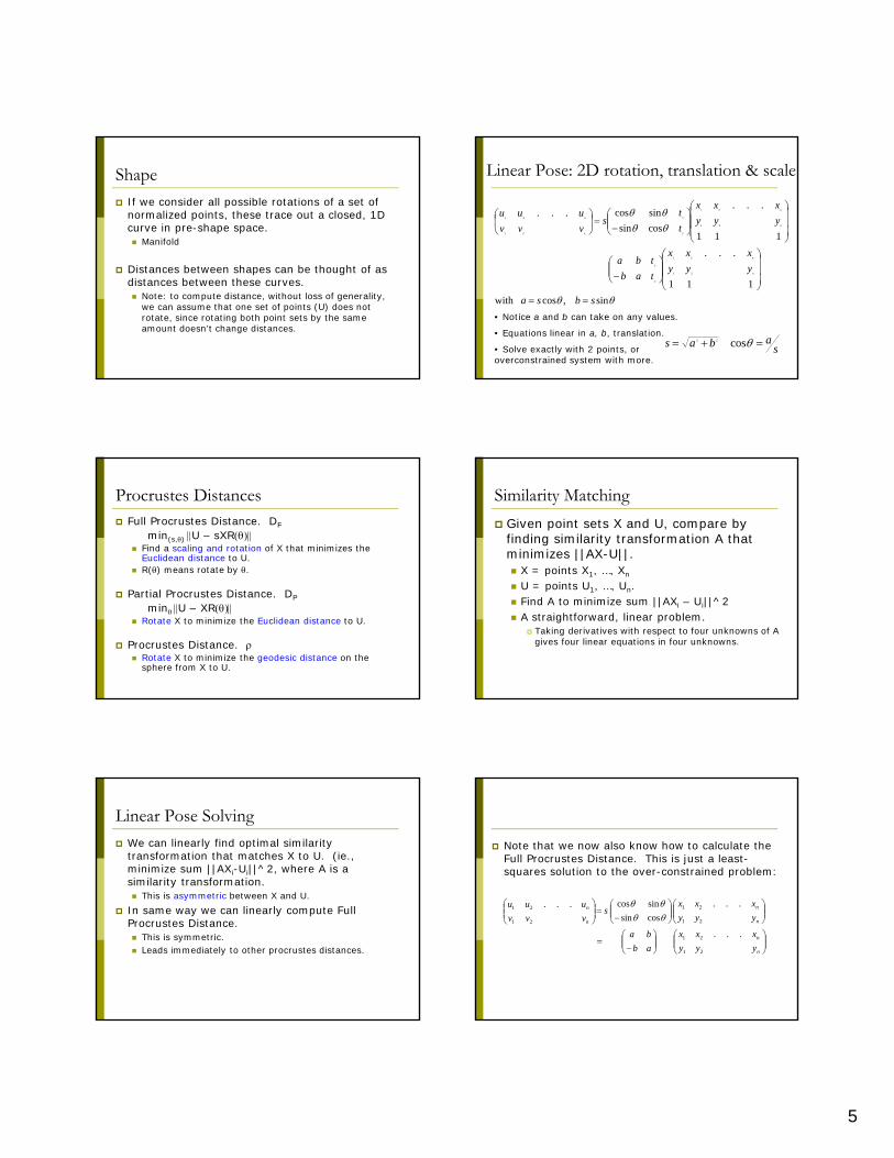
Articulation Invariant Shape Matching

PAMI’07, Ling & Jacobs

Inner-distanceLength of the shortest path between landmark points.

Articulation InsensitivityTheorem: The change of inner-distances during articulation is up bounded by a small value.

ComputationShortest pathFast marching

Inner-Distance, Articulation Insensitivity

Computation:Step 1: Build graph

Points NodesVisible point pairs Edges

Step 2: Shortest pathE.g., Bellman-Ford

0

00

3

9

0

5

3

0

13

0

110 0

5

10

40

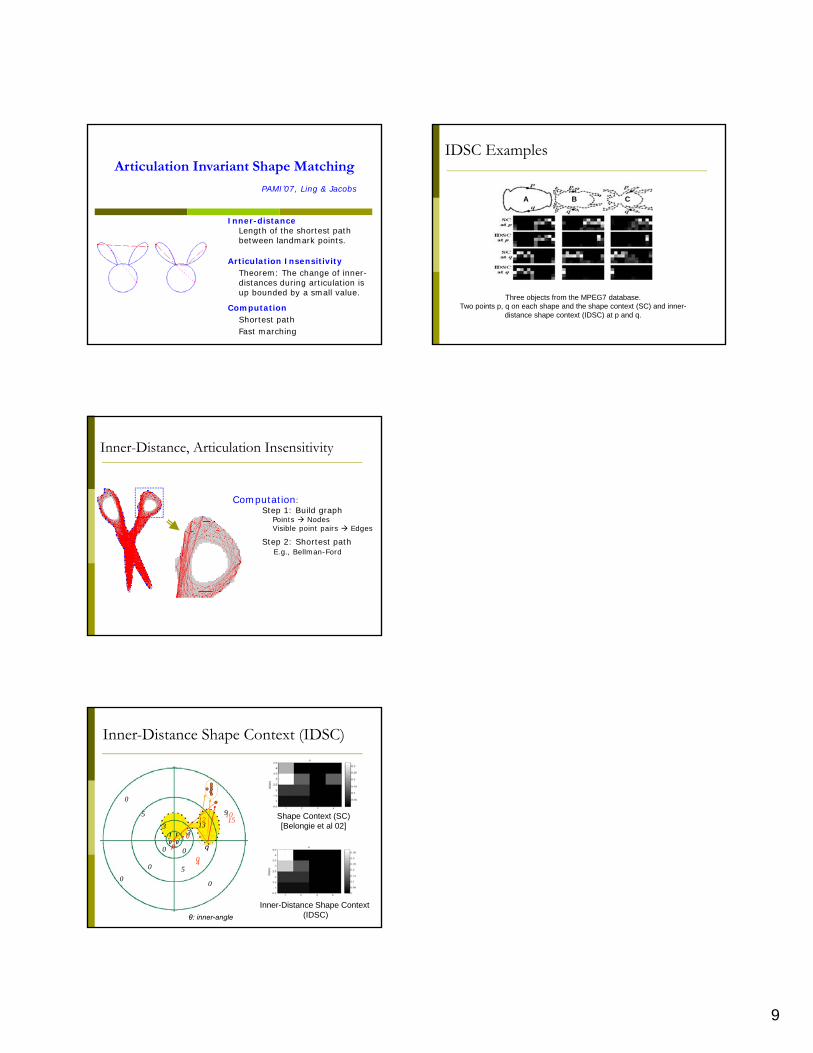
12 15 Shape Context (SC)[Belongie et al 02]

Inner-Distance Shape Context (IDSC)

q

θ

Inner-Distance Shape Context (IDSC)

p

θ: inner-angle

IDSC Examples

Three objects from the MPEG7 database. Two points p, q on each shape and the shape context (SC) and inner-

distance shape context (IDSC) at p and q.

A B C