Receptivity of Boundary-Layer Flowsover Flat and Curved Walls

by

Lars-Uve Schrader

November 2010Technical Reports

KTH Royal Institute of TechnologyLinne Flow Centre, KTH Mechanics

SE-100 44 Stockholm, Sweden

Akademisk avhandling som med tillstand av Kungliga Tekniska Hogskolan iStockholm framlagges till offentlig granskning for avlaggande av teknologiedoktorsexamen fredagen den 12 november 2010 kl 10.00 i sal F3, KungligaTekniska Hogskolan, Lindstedtsvagen 26, Stockholm.

c⃝Lars-Uve Schrader 2010

Universitetsservice US–AB, Stockholm 2010

Receptivity of Boundary-Layer Flows over Flat and CurvedWalls

Lars-Uve SchraderLinne Flow CentreKTH Mechanics, KTH Royal Institute of TechnologySE-100 44 Stockholm, Sweden

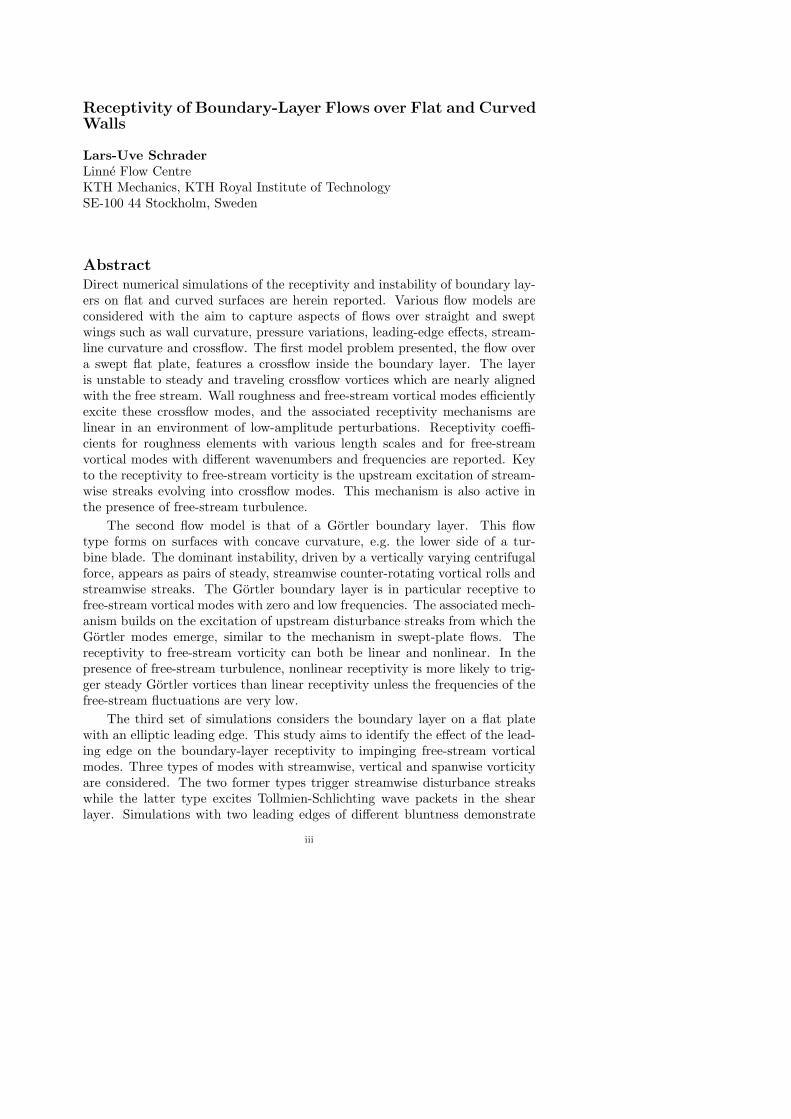
AbstractDirect numerical simulations of the receptivity and instability of boundary lay-ers on flat and curved surfaces are herein reported. Various flow models areconsidered with the aim to capture aspects of flows over straight and sweptwings such as wall curvature, pressure variations, leading-edge effects, stream-line curvature and crossflow. The first model problem presented, the flow overa swept flat plate, features a crossflow inside the boundary layer. The layeris unstable to steady and traveling crossflow vortices which are nearly alignedwith the free stream. Wall roughness and free-stream vortical modes efficientlyexcite these crossflow modes, and the associated receptivity mechanisms arelinear in an environment of low-amplitude perturbations. Receptivity coeffi-cients for roughness elements with various length scales and for free-streamvortical modes with different wavenumbers and frequencies are reported. Keyto the receptivity to free-stream vorticity is the upstream excitation of stream-wise streaks evolving into crossflow modes. This mechanism is also active inthe presence of free-stream turbulence.

The second flow model is that of a Gortler boundary layer. This flowtype forms on surfaces with concave curvature, e.g. the lower side of a tur-bine blade. The dominant instability, driven by a vertically varying centrifugalforce, appears as pairs of steady, streamwise counter-rotating vortical rolls andstreamwise streaks. The Gortler boundary layer is in particular receptive tofree-stream vortical modes with zero and low frequencies. The associated mech-anism builds on the excitation of upstream disturbance streaks from which theGortler modes emerge, similar to the mechanism in swept-plate flows. Thereceptivity to free-stream vorticity can both be linear and nonlinear. In thepresence of free-stream turbulence, nonlinear receptivity is more likely to trig-ger steady Gortler vortices than linear receptivity unless the frequencies of thefree-stream fluctuations are very low.

The third set of simulations considers the boundary layer on a flat platewith an elliptic leading edge. This study aims to identify the effect of the lead-ing edge on the boundary-layer receptivity to impinging free-stream vorticalmodes. Three types of modes with streamwise, vertical and spanwise vorticityare considered. The two former types trigger streamwise disturbance streakswhile the latter type excites Tollmien-Schlichting wave packets in the shearlayer. Simulations with two leading edges of different bluntness demonstrate

iii

that the leading-edge shape hardly influences the receptivity to streamwise vor-tices, whereas it significantly enhances the receptivity to vertical and spanwisevortices. It is shown that the receptivity mechanism to vertical free-streamvorticity involves vortex stretching and tilting – physical processes which areclearly enhanced by blunt leading edges.

The last flow configuration studied models an infinite wing at 45 degreessweep. This model is the least idealized with respect to applications in aerospaceengineering. The set-up mimics the wind-tunnel experiments carried out bySaric and coworkers at the Arizona State University in the 1990s. The numer-ical method is verified by simulating the excitation of steady crossflow vorticesthrough micron-sized roughness as realized in the experiments. Moreover, thereceptivity to free-stream vortical disturbances is investigated and it is shownthat the boundary layer is most receptive if the free-stream modes are closelyaligned with the most unstable crossflow mode.

DescriptorsBoundary-layer receptivity, laminar-turbulent transition, swept-plate boundarylayer, Gortler flow, leading-edge effects, swept-wing flow, crossflow vortices,Gortler rolls, disturbance streaks, wall roughness, free-stream turbulence

iv

Preface

This thesis deals with the receptivity, instability and transition to turbulence inspatially developing boundary layers on flat and curved walls. These physicalprocesses were investigated using direct numerical simulation. A brief overviewover the basic concepts and numerical methods is presented in the first part.The second part is a collection of the articles listed below. Papers 1 to 4 appearhere in the same form as the corresponding submitted and published versionsexcept for some adjustments to the present thesis format and a few correctionsof errata. Papers 5 and 6 are internal technical reports.

Paper 1L.-U. Schrader, L. Brandt & D.S. Henningson, 2009Receptivity mechanisms in three-dimensional boundary-layer flows.J. Fluid Mech. 618, pp. 209–241

Paper 2L.-U. Schrader, S. Amin & L. Brandt, 2010Transition to turbulence in the boundary layer over a smooth and rough sweptplate exposed to free-stream turbulence. J. Fluid Mech. 646, pp. 297–325

Paper 3L.-U. Schrader, L. Brandt & T. A. Zaki, 2010Receptivity, instability and breakdown of Gortler flow.Submitted to J. Fluid Mech.

Paper 4L.-U. Schrader, L. Brandt, C. Mavriplis & D. S. Henningson, 2010Receptivity to free-stream vorticity of flow past a flat plate with elliptic leadingedge. J. Fluid Mech. 653, pp. 245–271

Paper 5L.-U. Schrader, 2010Nonlinear receptivity of leading-edge flow to oblique free-stream vortical modes.Internal report

Paper 6L.-U. Schrader, D. Tempelmann, L. Brandt,A. Hanifi & D. S. Henningson, 2010Numerical study of boundary-layer receptivity on a swept wing.Internal report

v

Authors’ contributions to the papersThe research project was initiated by Dr. Luca Brandt (LB) who is Lars-UveSchrader’s (LS) main advisor. Prof. Dan Henningson (DH) acts as the co-advisor. In 2009 LB initiated a collaboration with Prof. Tamer Zaki (TZ)from Imperial College London, UK. As a result, LS spent six months with TZ’sresearch group.

Paper 1The modification of the simulation code and the computations were performedby LS with feedback from LB. Most of the paper was written by LS with inputfrom LB and DH.

Paper 2LS carried out the implementation of the surface roughness and the adaptationof the free-stream turbulence code to three-dimensional flows. The simulationswere performed by Subir Amin as a part of his Master’s Thesis and by LS.Most parts of the paper were written by LS with the help of LB, who wrotethe section about the breakdown.

Paper 3LS carried out the receptivity calculations using the open-source spectral ele-ment code Nek5000 (Argonne National Laboratory, USA). TZ performed thesimulations of laminar-turbulent transition due to free-stream turbulence. LSanalyzed the data and wrote the manuscript with the help of TZ and LB.

Paper 4The spectral element code Nek5000 was used. LS modified parts of the codefor the handling of the computational mesh and the boundary conditions withthe help of Prof. Catherine Mavriplis (CM). LS performed the computationsand wrote the paper with inputs from LB, CM and DH.

Paper 5LS carried out the simulations, using the code Nek5000, and wrote the report.

Paper 6LS and David Tempelmann (DT) developed the computational meshes. Theinitial and boundary conditions were extracted from RANS simulations byArdeshir Hanifi (AH). The simulations were performed by LS and DT, us-ing Nek5000. The report was written by LS with inputs from LB, DT, AH andDH.

vi

Abstract iii

Preface v

Part I – Introduction 1

Chapter 1. Introduction 2

1.1. Boundary layer 2

1.2. Receptivity 3

1.3. Instability 3

1.4. Breakdown to turbulence 4

Chapter 2. Boundary-layer flows 5

2.1. Characteristic scales 5

2.2. Flow over wings 6

2.3. Model problems 8

2.3.1. Swept-plate flow 8

2.3.2. Flow over concave plates 10

2.3.3. Flow past elliptic leading edges 11

2.3.4. Swept-wing flow 13

Chapter 3. Instability 15

3.1. Linearized stability equations 15

3.2. Linear stability theory 16

3.3. Two examples of modal boundary-layer instability 18

3.3.1. Crossflow instability 18

3.3.2. Gortler instability 20

3.4. Nonmodal stability theory 22

3.5. An example: Boundary-layer streaks 23

Chapter 4. Receptivity 25

4.1. Receptivity coefficients 26

4.2. Examples of boundary-layer receptivity 28

4.2.1. Direct receptivity of swept-plate flow to roughness 28

4.2.2. Receptivity to vertical vorticity at a leading edge 29

4.2.3. Nonlinear receptivity of Gortler flow to free-stream vorticity 31

Chapter 5. Breakdown 33

5.1. Examples of secondary instability and breakdown 33

5.1.1. Streak instability in flat-plate flows 33

5.1.2. Secondary instability of Gortler rolls 34

vii

5.1.3. Turbulent spots in swept-plate flows 35

Chapter 6. Numerical methods 37

6.1. Direct numerical simulation 37

6.2. Simulation codes 38

6.3. Comparison 40

Chapter 7. Summary and outlook 42

Acknowledgements 44

Bibliography 47

Part II – Papers 51

Paper 1. Receptivity mechanisms in three-dimensional boundary-layer flows 55

Paper 2. Transition to turbulence in the boundary layer overa smooth and rough swept plate exposed to free-stream turbulence 97

Paper 3. Receptivity, instability and breakdown of Gortler flow 135

Paper 4. Receptivity to free-stream vorticity of flow past a flatplate with elliptic leading edge 183

Paper 5. Nonlinear receptivity of leading-edge flow to obliquefree-stream vortical modes 219

Paper 6. Numerical study of boundary-layer receptivity on aswept wing 237

1

Part I

Introduction

CHAPTER 1

Introduction

The present thesis reports numerical studies of the receptivity, instability andbreakdown to turbulence of boundary-layer flows over flat and curved surfaces.Obviously, the notions ‘boundary layer’, ‘receptivity’, ‘instability’ and ‘break-down’ play a central role for the current work. These are briefly introducedhere and explained in more detail in §§2, 4, 3 and 5, respectively.

1.1. Boundary layer

The boundary-layer concept is closely related with the internal friction in a flowfield due to the viscosity of the fluid. Already Newton described in his PrincipiaMathematica (1687) that the friction force per unit area (the shear stress τ)behaves as τ = −µ(du/dy) for one-dimensional flows, where µ stands for theviscosity and du/dy is the gradient of the flow velocity. Before the 20th centuryit was believed that τ is negligible in Newtonian fluids because of the very lowviscosity of these fluids (air: µ ∼ 10−5). This assumption led to the result thata solid body moving relative to a fluid does not experience a drag force. Thisis clearly against intuition, experience and experimental evidence, as alreadynoticed by d’Alembert in the mid of the 18th century. About 150 years laterthe German physicist Ludwig Prandtl was able to resolve d’Alembert’s paradoxby introducing the concept of boundary layer (Prandtl 1905). This is a verythin fluid layer on the surface of a body in a flow, for instance a wing in anairstream (see figure 1.1a). Prandtl assumed that the fluid sticks to the wallof the body (no slip) where the flow velocity – for a fixed body – hence iszero, and that the velocity increases from zero to the value of the free streamacross a very thin layer. Thus, the wall-normal component of ∇u becomeslarge inside the boundary layer and the shear stress is relevant even in fluidswith low viscosity. In particular, the shear stress at the wall exerts a drag forceon the body, the skin-friction drag. The boundary-layer theory thus offered anexplanation for the conventional wisdom that a body moving through a fluidexperiences a force. Outside the boundary layer, where both µ and ∇u aresmall, the flow behaves essentially as an inviscid flow.

The flow in the boundary layer may be smooth and ordered (laminar) orswirling and chaotic (turbulent). On an airplane wing, for instance, the flowstarts out as laminar at the leading edge. At some location downstream of theleading edge, the laminar flow becomes unstable and turns into a turbulentmotion. The boundary layer is said to undergo a laminar-turbulent transition.

2

1.3. INSTABILITY 3

(a) (b)

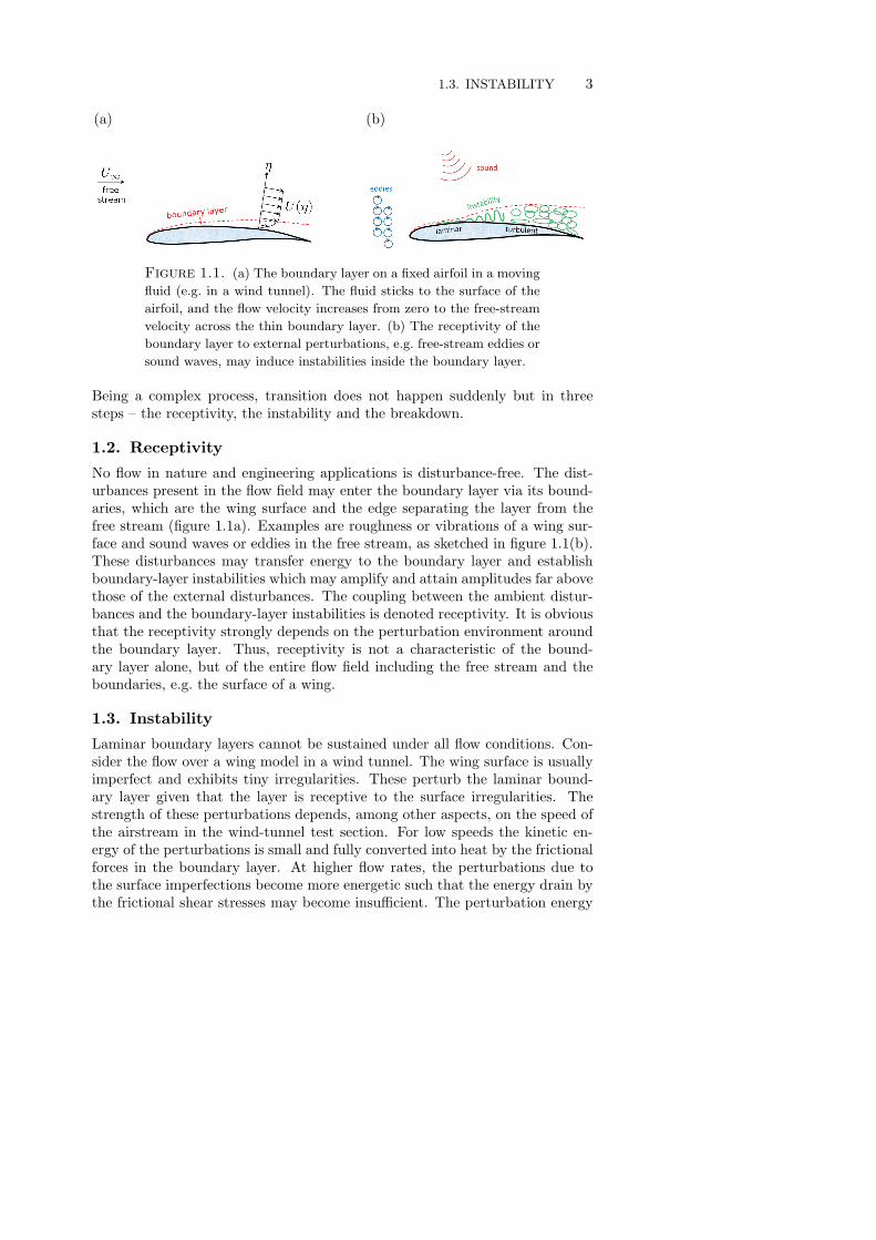
Figure 1.1. (a) The boundary layer on a fixed airfoil in a moving

fluid (e.g. in a wind tunnel). The fluid sticks to the surface of the

airfoil, and the flow velocity increases from zero to the free-stream

velocity across the thin boundary layer. (b) The receptivity of the

boundary layer to external perturbations, e.g. free-stream eddies or

sound waves, may induce instabilities inside the boundary layer.

Being a complex process, transition does not happen suddenly but in threesteps – the receptivity, the instability and the breakdown.

1.2. Receptivity

No flow in nature and engineering applications is disturbance-free. The dist-urbances present in the flow field may enter the boundary layer via its bound-aries, which are the wing surface and the edge separating the layer from thefree stream (figure 1.1a). Examples are roughness or vibrations of a wing sur-face and sound waves or eddies in the free stream, as sketched in figure 1.1(b).These disturbances may transfer energy to the boundary layer and establishboundary-layer instabilities which may amplify and attain amplitudes far abovethose of the external disturbances. The coupling between the ambient distur-bances and the boundary-layer instabilities is denoted receptivity. It is obviousthat the receptivity strongly depends on the perturbation environment aroundthe boundary layer. Thus, receptivity is not a characteristic of the bound-ary layer alone, but of the entire flow field including the free stream and theboundaries, e.g. the surface of a wing.

1.3. Instability

Laminar boundary layers cannot be sustained under all flow conditions. Con-sider the flow over a wing model in a wind tunnel. The wing surface is usuallyimperfect and exhibits tiny irregularities. These perturb the laminar bound-ary layer given that the layer is receptive to the surface irregularities. Thestrength of these perturbations depends, among other aspects, on the speed ofthe airstream in the wind-tunnel test section. For low speeds the kinetic en-ergy of the perturbations is small and fully converted into heat by the frictionalforces in the boundary layer. At higher flow rates, the perturbations due tothe surface imperfections become more energetic such that the energy drain bythe frictional shear stresses may become insufficient. The perturbation energy

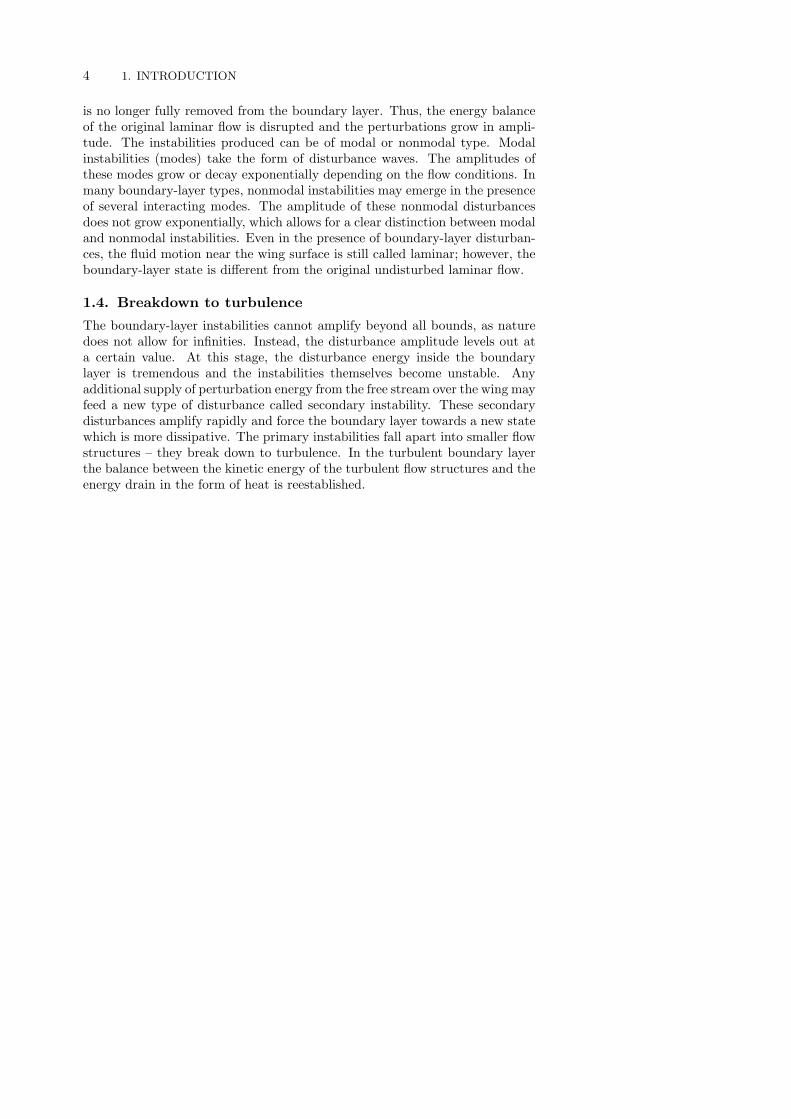
4 1. INTRODUCTION

is no longer fully removed from the boundary layer. Thus, the energy balanceof the original laminar flow is disrupted and the perturbations grow in ampli-tude. The instabilities produced can be of modal or nonmodal type. Modalinstabilities (modes) take the form of disturbance waves. The amplitudes ofthese modes grow or decay exponentially depending on the flow conditions. Inmany boundary-layer types, nonmodal instabilities may emerge in the presenceof several interacting modes. The amplitude of these nonmodal disturbancesdoes not grow exponentially, which allows for a clear distinction between modaland nonmodal instabilities. Even in the presence of boundary-layer disturban-ces, the fluid motion near the wing surface is still called laminar; however, theboundary-layer state is different from the original undisturbed laminar flow.

1.4. Breakdown to turbulence

The boundary-layer instabilities cannot amplify beyond all bounds, as naturedoes not allow for infinities. Instead, the disturbance amplitude levels out ata certain value. At this stage, the disturbance energy inside the boundarylayer is tremendous and the instabilities themselves become unstable. Anyadditional supply of perturbation energy from the free stream over the wing mayfeed a new type of disturbance called secondary instability. These secondarydisturbances amplify rapidly and force the boundary layer towards a new statewhich is more dissipative. The primary instabilities fall apart into smaller flowstructures – they break down to turbulence. In the turbulent boundary layerthe balance between the kinetic energy of the turbulent flow structures and theenergy drain in the form of heat is reestablished.

CHAPTER 2

Boundary-layer flows

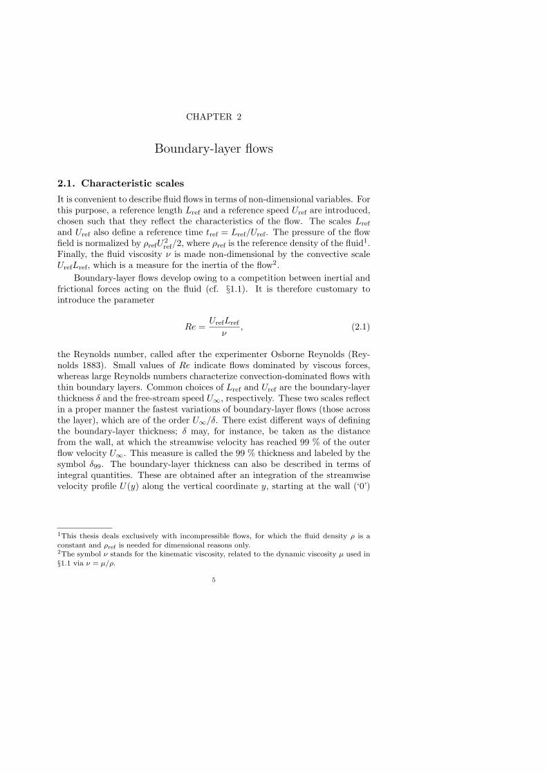
2.1. Characteristic scales

It is convenient to describe fluid flows in terms of non-dimensional variables. Forthis purpose, a reference length Lref and a reference speed Uref are introduced,chosen such that they reflect the characteristics of the flow. The scales Lref

and Uref also define a reference time tref = Lref/Uref. The pressure of the flowfield is normalized by ρrefU

2ref/2, where ρref is the reference density of the fluid1.

Finally, the fluid viscosity ν is made non-dimensional by the convective scaleUrefLref, which is a measure for the inertia of the flow2.

Boundary-layer flows develop owing to a competition between inertial andfrictional forces acting on the fluid (cf. §1.1). It is therefore customary tointroduce the parameter

Re =UrefLref

ν, (2.1)

the Reynolds number, called after the experimenter Osborne Reynolds (Rey-nolds 1883). Small values of Re indicate flows dominated by viscous forces,whereas large Reynolds numbers characterize convection-dominated flows withthin boundary layers. Common choices of Lref and Uref are the boundary-layerthickness δ and the free-stream speed U∞, respectively. These two scales reflectin a proper manner the fastest variations of boundary-layer flows (those acrossthe layer), which are of the order U∞/δ. There exist different ways of definingthe boundary-layer thickness; δ may, for instance, be taken as the distancefrom the wall, at which the streamwise velocity has reached 99 % of the outerflow velocity U∞. This measure is called the 99 % thickness and labeled by thesymbol δ99. The boundary-layer thickness can also be described in terms ofintegral quantities. These are obtained after an integration of the streamwisevelocity profile U(y) along the vertical coordinate y, starting at the wall (‘0’)

1This thesis deals exclusively with incompressible flows, for which the fluid density ρ is aconstant and ρref is needed for dimensional reasons only.2The symbol ν stands for the kinematic viscosity, related to the dynamic viscosity µ used in§1.1 via ν = µ/ρ.

5

6 2. BOUNDARY-LAYER FLOWS

and reaching far out into the free stream (‘∞’),

δ∗ =

∞∫0

(1− U(y)

U∞

)dy,

θ =

∞∫0

U(y)

U∞

(1− U(y)

U∞

)dy. (2.2)

The thicknesses δ∗ and θ are the displacement thickness and the momentum-loss thickness of the boundary layer, respectively. These are illustrated infigure 2.1 for the example of a Blasius profile. Blasius flow is the boundary-layer flow over an infinitely thin flat plate downstream of the plate leadingedge (zero pressure gradient). The displacement thickness is the distance, bywhich a hypothetical inviscid-flow profile must be shifted away from the wall inorder to obtain the same volume flux as for the boundary-layer profile (figure2.1a). Analogously, the momentum-loss thickness corresponds to the distance,by which an inviscid-flow profile must be shifted away from the wall in order toobtain the same transport of streamwise momentum as for the boundary-layerprofile (figure 2.1b). The displacement thickness is often used to define theReynolds number, i.e. Re = U∞δ

∗/ν. In §2.3, we will also consider alternativedefinitions of Re.

0 0.4 0.8 1.20

2

4

6

8

U(y)

y

δ*

(a)

0 0.4 0.8 1.20

2

4

6

8

U(y)

y

θ

(b)

Figure 2.1. (a) The displacement thickness and (b) the

momentum-loss thickness of a Blasius profile.

2.2. Flow over wings

Figure 2.2 sketches the flow over a straight and a swept wing. Straight wingsare preferable for low-speed flight due to the beneficial lift performance atlow velocities. An example of a modern aircraft with straight wings is theBombardier Dash 8 Q400 (cruise speed 650 km/h). In contrast, high-speedairliners usually have swept wings. The sweep of the wing shifts the formationof shock waves at the wing leading edge towards speeds above those typical forcruising flight, thus avoiding an increase of resistance due to wave drag. The

2.2. FLOW OVER WINGS 7

Boeing 777 (cruise speed 900 km/h), with a wing sweepback of about 32◦, shallserve as an example here.

x

y

(a) (b)

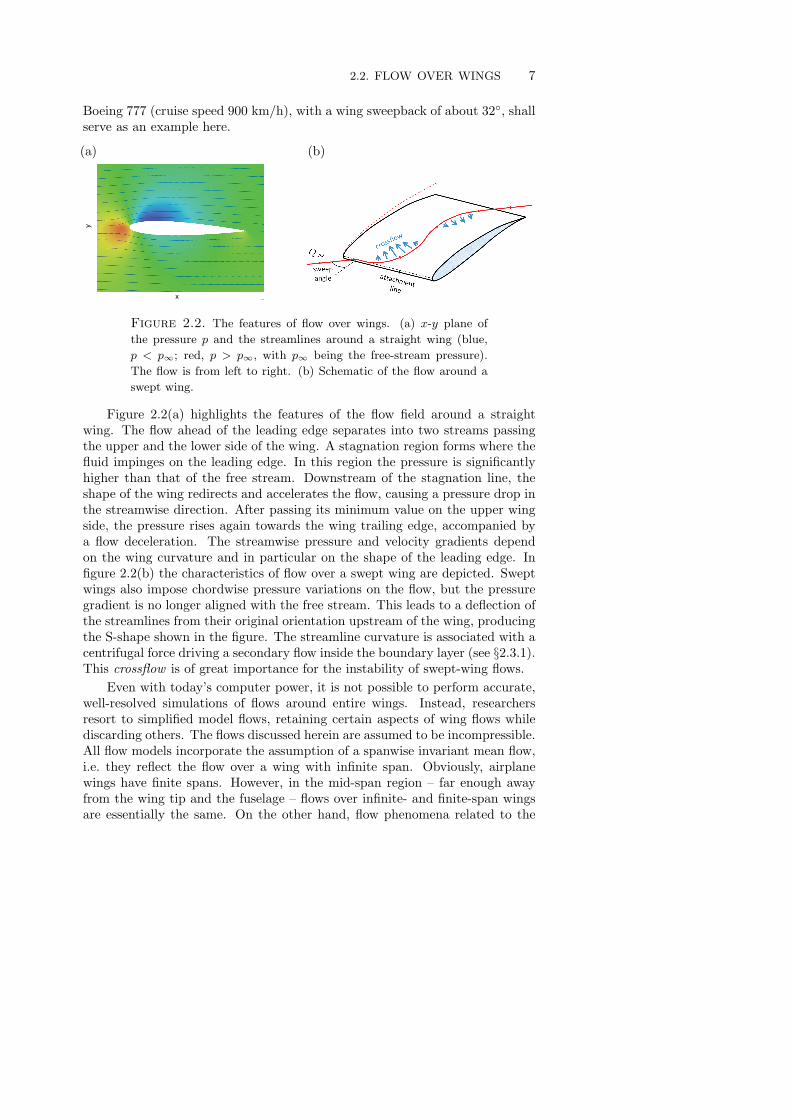
Figure 2.2. The features of flow over wings. (a) x-y plane of

the pressure p and the streamlines around a straight wing (blue,

p < p∞; red, p > p∞, with p∞ being the free-stream pressure).

The flow is from left to right. (b) Schematic of the flow around a

swept wing.

Figure 2.2(a) highlights the features of the flow field around a straightwing. The flow ahead of the leading edge separates into two streams passingthe upper and the lower side of the wing. A stagnation region forms where thefluid impinges on the leading edge. In this region the pressure is significantlyhigher than that of the free stream. Downstream of the stagnation line, theshape of the wing redirects and accelerates the flow, causing a pressure drop inthe streamwise direction. After passing its minimum value on the upper wingside, the pressure rises again towards the wing trailing edge, accompanied bya flow deceleration. The streamwise pressure and velocity gradients dependon the wing curvature and in particular on the shape of the leading edge. Infigure 2.2(b) the characteristics of flow over a swept wing are depicted. Sweptwings also impose chordwise pressure variations on the flow, but the pressuregradient is no longer aligned with the free stream. This leads to a deflection ofthe streamlines from their original orientation upstream of the wing, producingthe S-shape shown in the figure. The streamline curvature is associated with acentrifugal force driving a secondary flow inside the boundary layer (see §2.3.1).This crossflow is of great importance for the instability of swept-wing flows.

Even with today’s computer power, it is not possible to perform accurate,well-resolved simulations of flows around entire wings. Instead, researchersresort to simplified model flows, retaining certain aspects of wing flows whilediscarding others. The flows discussed herein are assumed to be incompressible.All flow models incorporate the assumption of a spanwise invariant mean flow,i.e. they reflect the flow over a wing with infinite span. Obviously, airplanewings have finite spans. However, in the mid-span region – far enough awayfrom the wing tip and the fuselage – flows over infinite- and finite-span wingsare essentially the same. On the other hand, flow phenomena related to the

8 2. BOUNDARY-LAYER FLOWS

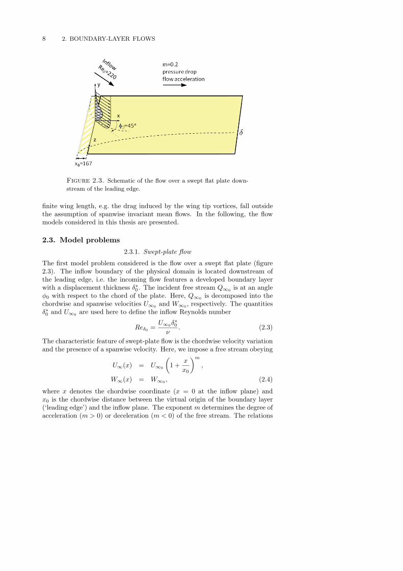
Figure 2.3. Schematic of the flow over a swept flat plate down-

stream of the leading edge.

finite wing length, e.g. the drag induced by the wing tip vortices, fall outsidethe assumption of spanwise invariant mean flows. In the following, the flowmodels considered in this thesis are presented.

2.3. Model problems

2.3.1. Swept-plate flow

The first model problem considered is the flow over a swept flat plate (figure2.3). The inflow boundary of the physical domain is located downstream ofthe leading edge, i.e. the incoming flow features a developed boundary layerwith a displacement thickness δ∗0 . The incident free stream Q∞0 is at an angleϕ0 with respect to the chord of the plate. Here, Q∞0 is decomposed into thechordwise and spanwise velocities U∞0 and W∞0 , respectively. The quantitiesδ∗0 and U∞0 are used here to define the inflow Reynolds number

Reδ0 =U∞0δ

∗0

ν. (2.3)

The characteristic feature of swept-plate flow is the chordwise velocity variationand the presence of a spanwise velocity. Here, we impose a free stream obeying

U∞(x) = U∞0

(1 +

x

x0

)m

,

W∞(x) = W∞0 , (2.4)

where x denotes the chordwise coordinate (x = 0 at the inflow plane) andx0 is the chordwise distance between the virtual origin of the boundary layer(‘leading edge’) and the inflow plane. The exponentm determines the degree ofacceleration (m > 0) or deceleration (m < 0) of the free stream. The relations

2.3. MODEL PROBLEMS 9

0 300 600 900

35

40

45

1

1.2

1.4

x

φ

8

U

8

U8φ 8

(a)

0 0.5 1 1.50

3

6

9

Q, 5C

y

x=10

100300600

1000

(b)

Figure 2.4. (a) Chordwise velocity (U∞) according to (2.4) and

streamline angle (ϕ∞) in the free stream (y = 25) versus the chord-

wise coordinate for m = 0.2. (b) Streamwise velocity profiles (thin

lines) and crossflow profiles (multiplied by 5; thick lines) at various

chordwise locations.

in (2.4) are those of Falkner-Skan-Cooke flow, allowing for a self-similar solutionof the mean-flow profiles (Falkner & Skan 1931; Cooke 1950). Note that theswept-plate flow is fully characterized by the values of Reδ0 , ϕ0 and m, whichare given in figure 2.3. The distance x0 follows from

x0 =m+ 1

2

Reδ0c2

, (2.5)

where c is a constant for self-similar boundary layers, which must be calculatednumerically. The value of the present swept-plate flow is c = 0.893

Figure 2.4 shows some important characteristics of swept-plate flows. Thechordwise acceleration of the free stream (m = 0.2) causes curved externalstreamlines with downstream decreasing streamline angles (figure 2.4a). Thestreamline curvature is associated with a centrifugal force on the fluid elements.If the flow field is decomposed into components parallel and normal to the ex-ternal streamlines, the profiles Q(y) and C(y) in figure 2.4(b) are obtained.These are the streamwise and crossflow velocities, respectively. The physicalexplanation of the crossflow is as follows. In the free stream, the centrifu-gal force is counterbalanced by the pressure force. Towards the wall, the flowis retarded and the centrifugal force decreases, whereas the pressure is essen-tially unaffected. The resulting force imbalance induces a secondary flow inthe cross-stream direction – the crossflow – which is maximum in the bulkof the boundary layer and vanishes at the layer edge. The crossflow profilesare crucial for the instability characteristics of swept-plate flows (see §3.3.1)and also play an important role in flows over swept wings. Therefore – andbecause of the availability of analytical baseflow profiles – swept-plate flows

3The constant c is the ratio between the displacement thickness and the Falkner-Skan length

scale, c = δ∗(x)/δFS(x). The Falkner-Skan length δFS(x) =√

2/(m + 1)√

νx/U∞ is used

to form the similarity variable η(x, y) = y/δFS(x). See paper 1 for details.

10 2. BOUNDARY-LAYER FLOWS

Figure 2.5. Schematic of the flow over a concave plate down-

stream of the leading edge.

of Falkner-Skan-Cooke type were extensively studied (Crouch 1993; Choudhari1994; Hogberg & Henningson 1998, for instance). On the other hand, the in-fluences of the leading edge and of the surface curvature of swept wings are notcaptured within this approximation.

2.3.2. Flow over concave plates

Figure 2.5 depicts the flow over a concave plate downstream of the leading edge.The boundary layer forming on the plate is known as the Gortler boundary layer(Gortler 1941). The prominent characteristic of Gortler flows is the presenceof a centrifugal force acting on the fluid in the wall-normal direction. Thespeed of the incoming free stream is U∞, and the boundary layer features adisplacement thickness of δ∗0 at the inflow plane of the physical domain. Thequantities U∞ and δ∗0 , chosen to be the reference length and speed, are used toformulate the inflow Reynolds number

Reδ0 =U∞0δ

∗0

ν. (2.6)

The flow is fully determined by Reδ0 and by the radius of curvature R of theplate, which are given in figure 2.5. Gortler (1941) introduced an alternativecontrol parameter, the Gortler number

Gθ =U∞0θ

ν

√θ

R= Reθ

√θ

R. (2.7)

Traditionally, the momentum-loss thickness θ rather than the displacementthickness δ∗ of the Gortler boundary layer is used in the definition of theGortler number. Gθ combines the Reynolds number (based on θ) with a non-dimensional curvature parameter. The flow over the concave plate is hence

2.3. MODEL PROBLEMS 11

0 0.05 0.1 0.15 0.20

30

60

90

(p−p )/(p0−p )

η

ξ=0

1504.5936

0.19 0.20

3

6

9

δ*

0

δ*(ξ=1505)

(a)

0 500 1000 15000

2

4

6

ξ

δ* , θ

δ*

θ

δ*

Blasius

θBlasius

(b)

Figure 2.6. (a) Wall-normal pressure distribution of Gortler flow.

(b) Displacement and momentum-loss thicknesses of the Gortler

boundary layer as compared with the Blasius boundary layer.

fully described by one single parameter (Gθ0) instead of two (Reδ0 and R),where Gθ0 is the inflow Gortler number

Gθ0 =U∞0θ0ν

√θ0R, (2.8)

with θ0 being the inflow momentum-loss thickness. The value of Gθ0 consideredhere is given in figure 2.5.

Figure 2.6(a) shows that the vertical pressure decreases away from the con-cave wall. This pressure distribution is a result of the increase of the balancingcentrifugal force in the wall-normal direction owing to a decrease of the radiusof the streamlines. The inset of figure 2.6(a) shows that the wall-normal pres-sure gradient relaxes towards zero inside the boundary layer, in agreement withthe vertical boundary-layer momentum equation ∂p/∂η = 0. The streamwisedevelopment of the boundary layer (e.g. its thicknesses) is hardly affected bythe presence of the wall-normal centrifugal force and essentially correspondsto that in Blasius flow (figure 2.6b). The Gortler boundary layer is a modelfor the flow past the concave regions of wings and blades. These regions areusually found on the lower side of the aerodynamic shape. Gortler flow is inparticular relevant on turbine blades. The present model incorporates the mostimportant aspects of these flows – the wall curvature and the resulting wall-normal centrifugal forces. Leading-edge effects are, however, excluded from ouranalysis.

2.3.3. Flow past elliptic leading edges

Figure 2.7 shows the third flow model considered. A flat plate with an ellipticleading edge serves as a model of a straight wing. The shape of the leadingedge is that of a modified super-ellipse (MSE, Lin et al. 1992). In contrast toa regular ellipse, the exponent p of the MSE (see inset of figure 2.7b) is not aconstant of two, but changes monotonically from two to three between the nose

12 2. BOUNDARY-LAYER FLOWS

(a) (b)

Figure 2.7. Schematic of the flow over a flat plate with an elliptic

leading edge.

of the leading edge and the joint to the flat plate. This guarantees that notonly the contour but also the slope and the curvature of the plate are smoothat the juncture. The shape of the leading edge can be altered by changingthe semi-major and semi-minor ellipse axes a and b, which are related witheach other via the leading-edge aspect ratio AR = a/b. A small value of ARindicates a blunt leading edge, whereas slender leading edges have a large AR.Here, the semi-minor axis b, which is also the half-thickness of the plate, shallserve as the reference length and the free stream velocity U∞ as the referencespeed of the flow. The Reynolds number is based on these two quantities,

Reb =U∞b

ν. (2.9)

It is also common to express the Reynolds number in terms of the streamwiselocation xout of the outflow boundary of the physical domain, i.e. Rexout =U∞xout/ν. The flow field around the plate is fully characterized by the valuesof Reb (or Rexout) and AR, which are given in figure 2.7.

Figure 2.8(a) shows the streamwise pressure variations for two differentplates with blunt (AR = 6) and slender leading edges (AR = 20). Downstreamof the stagnation line (cp = 1), the pressure drops rapidly, accompanied by astrong flow acceleration, and attains its minimum value (‘suction peak’) be-tween the nose and the junction of the leading edge. Subsequently, the fluidpasses a region of adverse pressure gradient where the flow decelerates. Far-ther downstream, on the flat part of the plate, the pressure relaxes towards aconstant value. Figure 2.8(b) shows that downstream of the leading-edge junc-ture, the wall vorticity of the flows over the plates with elliptic leading edgesconverges with that of the Blasius boundary layer. Many relevant aspects offlows around straight wings are included in the model flow over a flat plate withan elliptic leading edge, for instance the stagnation region, the attachment lineand the streamwise flow variations in the leading-edge vicinity. On the otherhand, the downstream pressure distribution is different from that on a wing,

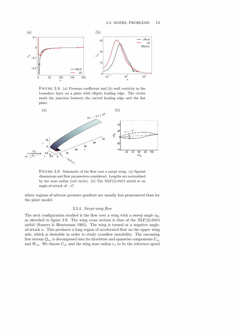
2.3. MODEL PROBLEMS 13

0 50 100 150 200

−0.2

−0.1

0

0.1

x

cp

AR=6

20

(a)

10−2

100

102

0

15

30

45

x

ζw

AR=6

20

Blasius

(b)

Figure 2.8. (a) Pressure coefficient and (b) wall vorticity in the

boundary layer on a plate with elliptic leading edge. The circles

mark the junction between the curved leading edge and the flat

plate.

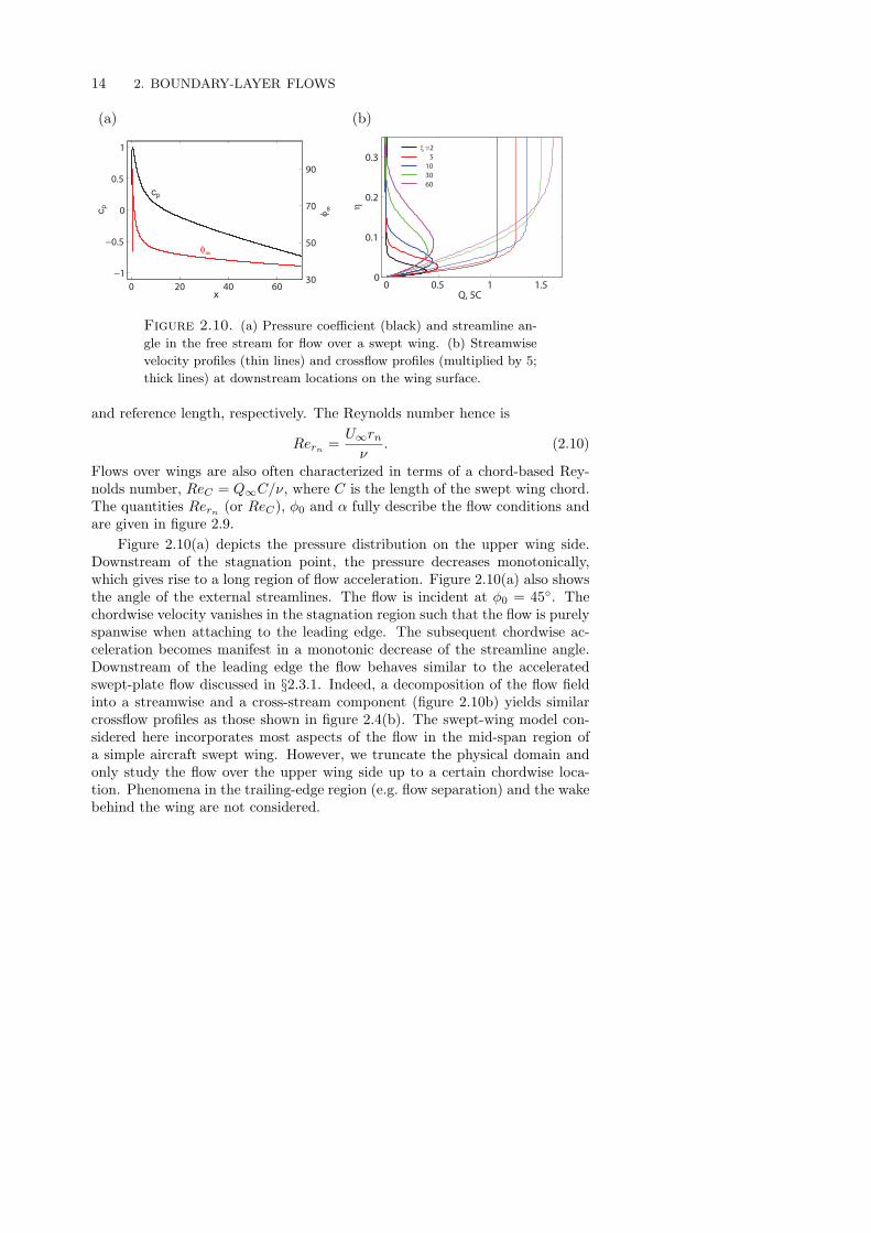
(a) (b)

Figure 2.9. Schematic of the flow over a swept wing. (a) Spatial

dimensions and flow parameters considered. Lengths are normalized

by the nose radius (red circle). (b) The NLF(2)-0415 airfoil at an

angle-of-attack of −4◦.

where regions of adverse pressure gradient are usually less pronounced than forthe plate model.

2.3.4. Swept-wing flow

The next configuration studied is the flow over a wing with a sweep angle ϕ0,as sketched in figure 2.9. The wing cross section is that of the NLF(2)-0415airfoil (Somers & Horstmann 1985). The wing is turned at a negative angle-of-attack α. This produces a long region of accelerated flow on the upper wingside, which is desirable in order to study crossflow instability. The oncomingfree stream Q∞ is decomposed into its chordwise and spanwise components U∞and W∞. We choose U∞ and the wing nose radius rn to be the reference speed

14 2. BOUNDARY-LAYER FLOWS

0 20 40 60

−1

−0.5

0

0.5

1

30

50

70

90

φ

8cp

φ 8

cp

x

(a)

0 0.5 1 1.50

0.1

0.2

0.3

Q, 5C

η

ξ =2

5

10

30

60

(b)

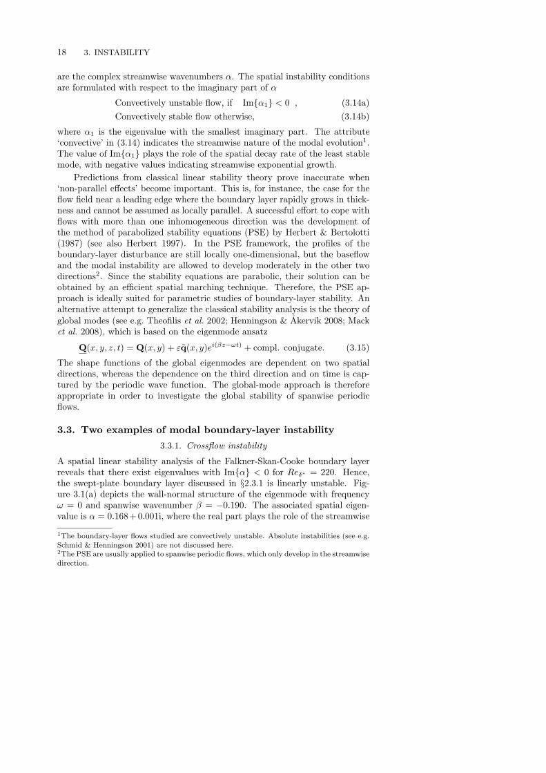
Figure 2.10. (a) Pressure coefficient (black) and streamline an-

gle in the free stream for flow over a swept wing. (b) Streamwise

velocity profiles (thin lines) and crossflow profiles (multiplied by 5;

thick lines) at downstream locations on the wing surface.

and reference length, respectively. The Reynolds number hence is

Rern =U∞rnν

. (2.10)

Flows over wings are also often characterized in terms of a chord-based Rey-nolds number, ReC = Q∞C/ν, where C is the length of the swept wing chord.The quantities Rern (or ReC), ϕ0 and α fully describe the flow conditions andare given in figure 2.9.

Figure 2.10(a) depicts the pressure distribution on the upper wing side.Downstream of the stagnation point, the pressure decreases monotonically,which gives rise to a long region of flow acceleration. Figure 2.10(a) also showsthe angle of the external streamlines. The flow is incident at ϕ0 = 45◦. Thechordwise velocity vanishes in the stagnation region such that the flow is purelyspanwise when attaching to the leading edge. The subsequent chordwise ac-celeration becomes manifest in a monotonic decrease of the streamline angle.Downstream of the leading edge the flow behaves similar to the acceleratedswept-plate flow discussed in §2.3.1. Indeed, a decomposition of the flow fieldinto a streamwise and a cross-stream component (figure 2.10b) yields similarcrossflow profiles as those shown in figure 2.4(b). The swept-wing model con-sidered here incorporates most aspects of the flow in the mid-span region ofa simple aircraft swept wing. However, we truncate the physical domain andonly study the flow over the upper wing side up to a certain chordwise loca-tion. Phenomena in the trailing-edge region (e.g. flow separation) and the wakebehind the wing are not considered.

CHAPTER 3

Instability

3.1. Linearized stability equations

The present study is restricted to incompressible boundary-layer flows. Theseflows are governed by the time-dependent incompressible Navier-Stokes equa-tions and the continuity condition,

∂U

∂t+ (U · ∇)U = −∇P +

1

Re∇2U, (3.1a)

∇ ·U = 0. (3.1b)

The instantaneous flow field (marked by an underline) is described by the ve-locity vector U(x, t) = (U, V ,W ) and the pressure P (x, t), which both dependon space x = (x, y, z) and time t. The equations in (3.1) are in non-dimensionalform, where velocities have been normalized by Uref and lengths by Lref, andRe = UrefLref/ν is the Reynolds number (cf. §2.1). The solution U(x, t) de-pends on the initial state of the flow field at time t0,

U(x, t0) = U0, (3.2)

and on the conditions at the boundaries of the physical domain. An exampleis the no-slip condition for the velocity at a solid wall.

The objective of a stability analysis is to determine the evolution of smalldisturbances u to the underlying baseflow U. If these disturbances grow inamplitude as time passes by (temporal perspective) or as they are advectedin downstream direction (spatial perspective), the boundary layer is unstable;if they, in contrast, decay, the flow is stable. The evolution of disturbancesis governed by the stability equations. These are derived by substituting thedecomposition

U = U+ εu, (3.3a)

P = P + εp (3.3b)

into (3.1), where P denotes the mean pressure and p the pressure perturbation.Within the framework of linear stability theory the disturbance amplitude ε in(3.3) is assumed to be small as compared with Uref. This allows for a lineariza-tion of the stability equations, i.e. the terms of order ε2 are discarded. After

15

16 3. INSTABILITY

subtracting the equations of the baseflow, we obtain

∂u

∂t+ (U · ∇)u+ (u · ∇)U = −∇p+ 1

Re∇2u, (3.4a)

∇ · u = 0. (3.4b)

The solution for u requires the specification of an initial state, e.g. adisturbance-free flow field, and of boundary conditions, for instance an incom-ing disturbance at the inflow boundary of the physical domain.

3.2. Linear stability theory

If the space and time variables are separable, the boundary-layer instabilitiescan be assumed as time-periodic. Then, (3.3) is written as

Q(x, y, z, t) = Q(x, y, z) + εq(x, y, z)e−iωt, (3.5)

where Q = (U, P ) and Q = (U, P ). The disturbance takes the form of atemporal Fourier mode with an amplitude function q = (u, p). In classicallinear theory, (3.5) is simplified by assuming a one-dimensional, locally parallelbaseflow and a disturbance with an amplitude function depending on the wall-normal direction only (‘normal mode’),

Q(x, y, z, t) = Q(y) + εq(y)ei(αx+βz−ωt) + compl. conjugate. (3.6)

This approach was in particular successful in viscous theory based on the Orr-Sommerfeld/Squire system (Orr 1907; Sommerfeld 1908; Squire 1933). Thenormal-mode ansatz is valid not only in strictly parallel flows (e.g. Couetteflow), but also in flows with a slow streamwise evolution. An example is thelaminar flat-plate boundary layer at large enough Reynolds numbers (Blasiusboundary layer). The normal modes of Blasius flow predicted by the lineartheory are referred to as Tollmien-Schlichting (T-S) waves. Instabilities of T-Stype were indeed observed in the wind-tunnel experiment on a flat plate bySchubauer & Skramstad (1947).

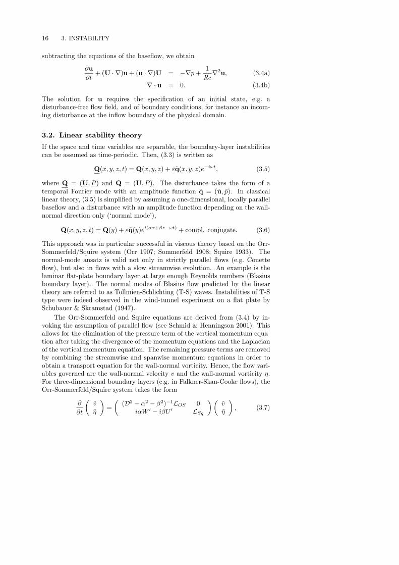
The Orr-Sommerfeld and Squire equations are derived from (3.4) by in-voking the assumption of parallel flow (see Schmid & Henningson 2001). Thisallows for the elimination of the pressure term of the vertical momentum equa-tion after taking the divergence of the momentum equations and the Laplacianof the vertical momentum equation. The remaining pressure terms are removedby combining the streamwise and spanwise momentum equations in order toobtain a transport equation for the wall-normal vorticity. Hence, the flow vari-ables governed are the wall-normal velocity v and the wall-normal vorticity η.For three-dimensional boundary layers (e.g. in Falkner-Skan-Cooke flows), theOrr-Sommerfeld/Squire system takes the form

∂

∂t

(vη

)=

((D2 − α2 − β2)−1LOS 0

iαW ′ − iβU ′ LSq

)(vη

), (3.7)

3.2. LINEAR STABILITY THEORY 17

where the tilde indicates a Fourier transformation to wavenumber space. Thelinear Orr-Sommerfeld and Squire operators LOS and LSq are

LOS = (−iαU − iβW )(D2 − α2 − β2) + iαU ′′ + iβW ′′ (3.8a)

+1

Re(D2 − α2 − β2)2,

LSq = −iαU − iβW +1

Re(D2 − α2 − β2). (3.8b)

The quantities α and β are the streamwise and spanwise wavenumbers, respec-tively, and D stands for the derivative operator in wall-normal direction. Theprime and double prime denote the first and second derivatives of the parallelbaseflow. The system (3.7) is an initial-value problem with the solution

q = eLtq|t=t0 , (3.9)

where q = (v, η), and L labels the matrix operator of (3.7). Key to a sta-bility analysis are the eigenvalues σi and the eigenfunctions ϕi of the matrixexponential

eLtϕi = σiϕi, |σ1| > · · · > |σn|. (3.10)

The instability condition stated in §3.1 can now be mathematically formulated:

Asymptotically unstable flow, if |σ1| > 1 , (3.11a)

Asymptotically stable flow otherwise. (3.11b)

The eigenvalues λi of of the matrix operator L are related with those of eLt viaλi = 1

t log σi. The values of λi are a measure for the temporal amplificationor decay rates of the eigenmodes ϕi. The conditions (3.11) indicate that oneeigenvalue alone governs the modal instability of the basic state, namely thatpertaining to the least stable eigenmode. The value of |σ1| determines whetherthe least stable mode grows beyond all bounds or decays to zero as time t→∞,i.e. it characterizes the asymptotic temporal stability of the baseflow.

In convection-dominated flows, the spatial stability is often more relevant.The spatial Orr-Sommerfeld/Sqire problem is formulated by re-ordering theterms of (3.7),

0 =

(LOS 0

iβU ′ − iαW ′ LSq

)(vη

), (3.12)

where LOS and LSq are the spatial Orr-Sommerfeld and Squire operators

LOS = (iω − iαU − iβW )(D2 − α2 − β2) + iαU ′′ + iβW ′′ (3.13a)

+1

Re(D2 − α2 − β2)2,

LSq = iω − iαU − iβW +1

Re(D2 − α2 − β2) (3.13b)

and ω is the angular frequency. The spatial stability of the basic state ischaracterized by the spatial eigenvalues of the operator matrix in (3.12), which

18 3. INSTABILITY

are the complex streamwise wavenumbers α. The spatial instability conditionsare formulated with respect to the imaginary part of α

Convectively unstable flow, if Im{α1} < 0 , (3.14a)

Convectively stable flow otherwise, (3.14b)

where α1 is the eigenvalue with the smallest imaginary part. The attribute‘convective’ in (3.14) indicates the streamwise nature of the modal evolution1.The value of Im{α1} plays the role of the spatial decay rate of the least stablemode, with negative values indicating streamwise exponential growth.

Predictions from classical linear stability theory prove inaccurate when‘non-parallel effects’ become important. This is, for instance, the case for theflow field near a leading edge where the boundary layer rapidly grows in thick-ness and cannot be assumed as locally parallel. A successful effort to cope withflows with more than one inhomogeneous direction was the development ofthe method of parabolized stability equations (PSE) by Herbert & Bertolotti(1987) (see also Herbert 1997). In the PSE framework, the profiles of theboundary-layer disturbance are still locally one-dimensional, but the baseflowand the modal instability are allowed to develop moderately in the other twodirections2. Since the stability equations are parabolic, their solution can beobtained by an efficient spatial marching technique. Therefore, the PSE ap-proach is ideally suited for parametric studies of boundary-layer stability. Analternative attempt to generalize the classical stability analysis is the theory ofglobal modes (see e.g. Theofilis et al. 2002; Henningson & Akervik 2008; Macket al. 2008), which is based on the eigenmode ansatz

Q(x, y, z, t) = Q(x, y) + εq(x, y)ei(βz−ωt) + compl. conjugate. (3.15)

The shape functions of the global eigenmodes are dependent on two spatialdirections, whereas the dependence on the third direction and on time is cap-tured by the periodic wave function. The global-mode approach is thereforeappropriate in order to investigate the global stability of spanwise periodicflows.

3.3. Two examples of modal boundary-layer instability

3.3.1. Crossflow instability

A spatial linear stability analysis of the Falkner-Skan-Cooke boundary layerreveals that there exist eigenvalues with Im{α} < 0 for Reδ∗ = 220. Hence,the swept-plate boundary layer discussed in §2.3.1 is linearly unstable. Fig-ure 3.1(a) depicts the wall-normal structure of the eigenmode with frequencyω = 0 and spanwise wavenumber β = −0.190. The associated spatial eigen-value is α = 0.168+0.001i, where the real part plays the role of the streamwise

1The boundary-layer flows studied are convectively unstable. Absolute instabilities (see e.g.Schmid & Henningson 2001) are not discussed here.2The PSE are usually applied to spanwise periodic flows, which only develop in the streamwisedirection.

3.3. TWO EXAMPLES OF MODAL BOUNDARY-LAYER INSTABILITY 19

0 1 2 3 4 50

2

4

6

8

|ui|

y

|u|

|v|

|w|

~

~

~

~

(a)

0 200 400 600 800−5

0

5

10x 10

−3

100

101

102

x

σe

e

σe

e

(b)

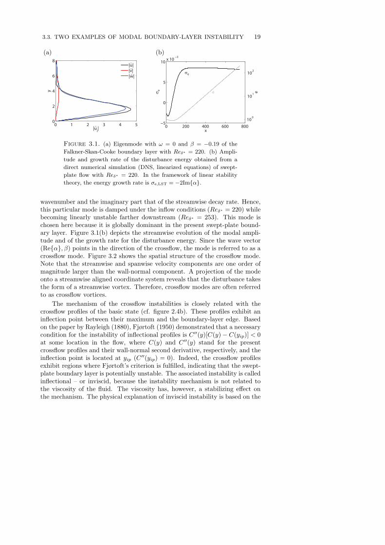
Figure 3.1. (a) Eigenmode with ω = 0 and β = −0.19 of the

Falkner-Skan-Cooke boundary layer with Reδ∗ = 220. (b) Ampli-

tude and growth rate of the disturbance energy obtained from a

direct numerical simulation (DNS, linearized equations) of swept-

plate flow with Reδ∗ = 220. In the framework of linear stability

theory, the energy growth rate is σe,LST = −2Im{α}.

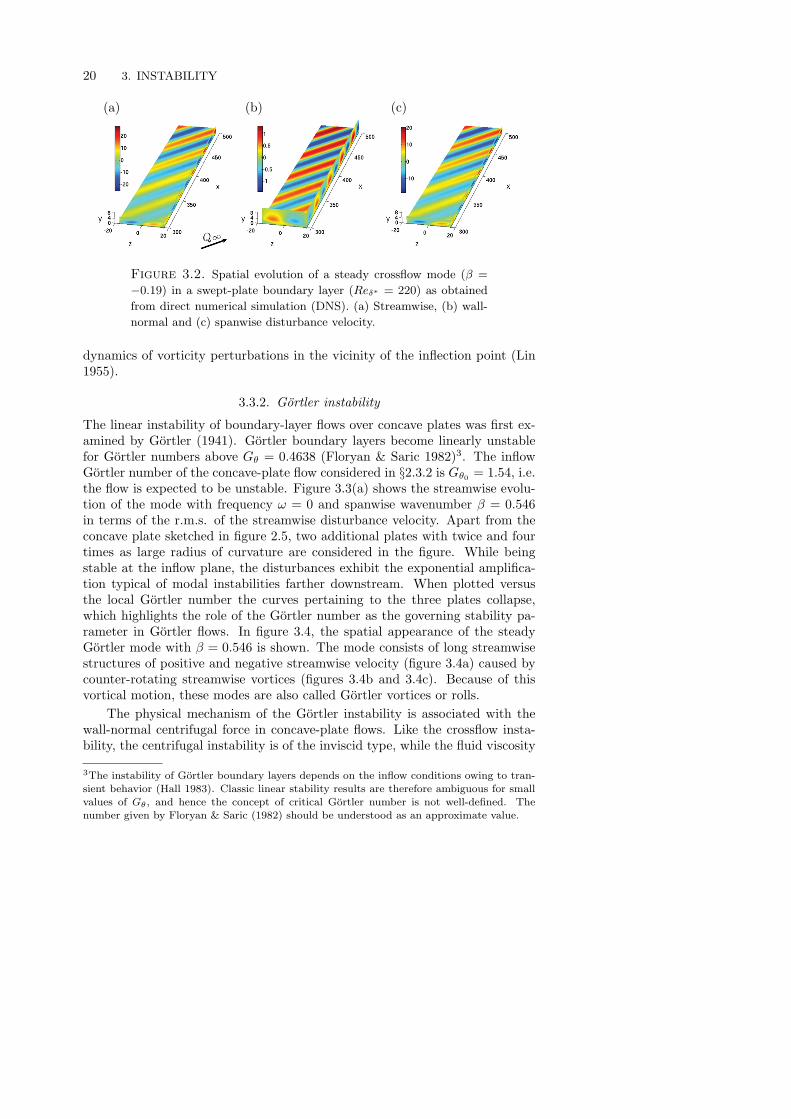
wavenumber and the imaginary part that of the streamwise decay rate. Hence,this particular mode is damped under the inflow conditions (Reδ∗ = 220) whilebecoming linearly unstable farther downstream (Reδ∗ = 253). This mode ischosen here because it is globally dominant in the present swept-plate bound-ary layer. Figure 3.1(b) depicts the streamwise evolution of the modal ampli-tude and of the growth rate for the disturbance energy. Since the wave vector(Re{α}, β) points in the direction of the crossflow, the mode is referred to as acrossflow mode. Figure 3.2 shows the spatial structure of the crossflow mode.Note that the streamwise and spanwise velocity components are one order ofmagnitude larger than the wall-normal component. A projection of the modeonto a streamwise aligned coordinate system reveals that the disturbance takesthe form of a streamwise vortex. Therefore, crossflow modes are often referredto as crossflow vortices.

The mechanism of the crossflow instabilities is closely related with thecrossflow profiles of the basic state (cf. figure 2.4b). These profiles exhibit aninflection point between their maximum and the boundary-layer edge. Basedon the paper by Rayleigh (1880), Fjørtoft (1950) demonstrated that a necessarycondition for the instability of inflectional profiles is C ′′(y)[C(y)− C(yip)] < 0at some location in the flow, where C(y) and C ′′(y) stand for the presentcrossflow profiles and their wall-normal second derivative, respectively, and theinflection point is located at yip (C ′′(yip) = 0). Indeed, the crossflow profilesexhibit regions where Fjørtoft’s criterion is fulfilled, indicating that the swept-plate boundary layer is potentially unstable. The associated instability is calledinflectional – or inviscid, because the instability mechanism is not related tothe viscosity of the fluid. The viscosity has, however, a stabilizing effect onthe mechanism. The physical explanation of inviscid instability is based on the

20 3. INSTABILITY

(a) (b) (c)

Figure 3.2. Spatial evolution of a steady crossflow mode (β =

−0.19) in a swept-plate boundary layer (Reδ∗ = 220) as obtained

from direct numerical simulation (DNS). (a) Streamwise, (b) wall-

normal and (c) spanwise disturbance velocity.

dynamics of vorticity perturbations in the vicinity of the inflection point (Lin1955).

3.3.2. Gortler instability

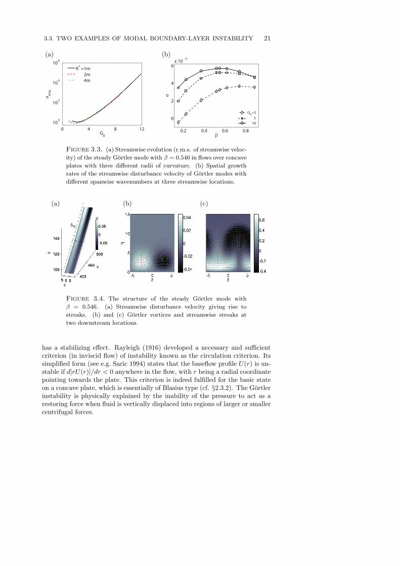
The linear instability of boundary-layer flows over concave plates was first ex-amined by Gortler (1941). Gortler boundary layers become linearly unstablefor Gortler numbers above Gθ = 0.4638 (Floryan & Saric 1982)3. The inflowGortler number of the concave-plate flow considered in §2.3.2 is Gθ0 = 1.54, i.e.the flow is expected to be unstable. Figure 3.3(a) shows the streamwise evolu-tion of the mode with frequency ω = 0 and spanwise wavenumber β = 0.546in terms of the r.m.s. of the streamwise disturbance velocity. Apart from theconcave plate sketched in figure 2.5, two additional plates with twice and fourtimes as large radius of curvature are considered in the figure. While beingstable at the inflow plane, the disturbances exhibit the exponential amplifica-tion typical of modal instabilities farther downstream. When plotted versusthe local Gortler number the curves pertaining to the three plates collapse,which highlights the role of the Gortler number as the governing stability pa-rameter in Gortler flows. In figure 3.4, the spatial appearance of the steadyGortler mode with β = 0.546 is shown. The mode consists of long streamwisestructures of positive and negative streamwise velocity (figure 3.4a) caused bycounter-rotating streamwise vortices (figures 3.4b and 3.4c). Because of thisvortical motion, these modes are also called Gortler vortices or rolls.

The physical mechanism of the Gortler instability is associated with thewall-normal centrifugal force in concave-plate flows. Like the crossflow insta-bility, the centrifugal instability is of the inviscid type, while the fluid viscosity

3The instability of Gortler boundary layers depends on the inflow conditions owing to tran-sient behavior (Hall 1983). Classic linear stability results are therefore ambiguous for small

values of Gθ, and hence the concept of critical Gortler number is not well-defined. Thenumber given by Floryan & Saric (1982) should be understood as an approximate value.

3.3. TWO EXAMPLES OF MODAL BOUNDARY-LAYER INSTABILITY 21

0 4

100

102

104

106

Gθ

urm

s

8 12

R* =1m

2m

4m

(a)

0.2 0.4 0.6 0.8

0

2

4

6x 10

−3

β

σ

Gθ

=3

5

10

(b)

Figure 3.3. (a) Streamwise evolution (r.m.s. of streamwise veloc-

ity) of the steady Gortler mode with β = 0.546 in flows over concave

plates with three different radii of curvature. (b) Spatial growth

rates of the streamwise disturbance velocity of Gortler modes with

different spanwise wavenumbers at three streamwise locations.

z

x

y

u

δ99

(a) (b) (c)

Figure 3.4. The structure of the steady Gortler mode with

β = 0.546. (a) Streamwise disturbance velocity giving rise to

streaks. (b) and (c) Gortler vortices and streamwise streaks at

two downstream locations.

has a stabilizing effect. Rayleigh (1916) developed a necessary and sufficientcriterion (in inviscid flow) of instability known as the circulation criterion. Itssimplified form (see e.g. Saric 1994) states that the baseflow profile U(r) is un-stable if d|rU(r)|/dr < 0 anywhere in the flow, with r being a radial coordinatepointing towards the plate. This criterion is indeed fulfilled for the basic stateon a concave plate, which is essentially of Blasius type (cf. §2.3.2). The Gortlerinstability is physically explained by the inability of the pressure to act as arestoring force when fluid is vertically displaced into regions of larger or smallercentrifugal forces.

22 3. INSTABILITY

3.4. Nonmodal stability theory

The wind-tunnel experiment by Schubauer & Skramstad (1947) gave strongsupport to the linear stability theory, which was apparently able to predictthe instability of flat-plate boundary layers. However, already the work byTaylor (1939) had cast a shadow on the classical approach. Later research ef-forts revealed that an eigenmode analysis fails to predict the response of theBlasius boundary layer to free-stream turbulence. Klebanoff (1971) observedboundary-layer disturbances in a wind-tunnel experiment which differed se-verely from the T-S waves predicted by a linear eigenmode analysis. Thesedisturbances occurred farther upstream, had a different shape and exhibited anon-exponential amplification rate. Since these instabilities are not associatedwith a single eigenmode of the baseflow, they are called nonmodal instabili-ties. The historical term ‘Klebanoff modes’ for these disturbances was coinedbefore their nonmodal nature was fully understood. The development of thenonmodal stability theory started with the paper by Ellingsen & Palm (1975)who demonstrated for inviscid shear layers that there exist initial disturban-ces growing linearly instead of exponentially in time. These disturbances werefound to produce a streaky pattern of alternating high and low streamwisevelocities. The amplification of the streaks was termed ‘transient growth’ byHultgren & Gustavsson (1981). Transient growth was shown to occur also inviscous flows.

The mathematical framework for transient growth was given by Butler& Farrell (1992); Reddy & Henningson (1993); Trefethen et al. (1993) (seealso Schmid & Henningson 2001). It is based on the non-normality of thelinear Navier-Stokes operator in shear flows (or of the Orr-Sommerfeld/Squireoperator discussed in §3). An operator L is non-normal if LL∗ = L∗L, wherethe star denotes the adjoint operator4. The transient growth of an initialdisturbance at time t = t0 is given by

G(t) = ∥eLtq|t=t0∥2. (3.16)

The condition for nonmodal instability is formulated by means of the singularvalues σi, which are the eigenvalues of the matrix eL

∗teLt,

eL∗teLtϕi = σiϕi, σ1 ≥ · · · ≥ σn ≥ 0. (3.17)

The condition for transient growth is stated as

Transient growth, if σ1 > 1, (3.18a)

No transient growth otherwise. (3.18b)

Transient amplification describes the short-time behavior of the boundary-layerdisturbances. In contrast, the linear growth is approached when t→∞, as re-flected by the attribute ‘asymptotic’ in (3.11). The instabilities undergoingtransient growth are nonmodal, because the underlying mechanism does not

4The adjoint operator is implicitly defined as the operator L∗ fulfilling ⟨Lx, y⟩ = ⟨x,L∗y⟩,where x, y ∈ H (Hilbert space) and ⟨·⟩ is an inner product defined on H.

3.5. AN EXAMPLE: BOUNDARY-LAYER STREAKS 23

0 100 200 300 4000

20

40

60

|uj |εj

x

0.72

β = 1.44

2.16

Figure 3.5. Streamwise amplification of steady boundary-layer

streaks with different spanwise wavenumbers in the flow over a plate

with an elliptic leading edge. Leading edges with aspect ratio AR =

6 (dashed lines) and AR = 20 (solid lines) are considered.

rely on the evolution of a single growing eigenmode. Instead, a linear interac-tion between eigenmodes of Orr-Sommerfeld and Squire type gives rise to thenonmodal instability. This results in a boundary-layer disturbance changing itsshape as individual modes grow or decay in time and space at different rates.Transient growth may for this reason occur before the subsequent exponentialbehavior and trigger the laminar-turbulent transition prior to the asymptoticinstability. The ‘natural transition mechanism’ due to the most unstable eigen-mode is then ‘bypassed’, and the transition route is called bypass transition.

3.5. An example: Boundary-layer streaks

Consider the boundary layer on the flat plate with an elliptic leading edgeintroduced in §2.3.3. When exposed to a free stream with vortical disturban-ces, this type of flow can develop nonmodal instabilities. Figure 3.5 shows thestreamwise evolution of nonmodal disturbances with frequency ω = 0 and threedifferent spanwise wavenumbers. Obviously, these instabilities do not amplifyexponentially in the downstream direction, which distinguishes them from theboundary-layer eigenmodes discussed in §3.3. Eventually, the nonmodal dist-urbances decay (cf. figure 3.5, β = 2.16), i.e. their amplification is limited inspace and time. Therefore, the evolution of nonmodal instabilities is referredto as transient (short-term) growth, as opposed to the asymptotic (long-term)behavior of the unstable eigenmodes of the flow. Figure 3.5 indicates that thetransient growth rate is substantial near the leading edge and that the am-plitude of the nonmodal instabilities can exceed the amplitude of their source(the free-stream disturbance here) by orders of magnitude. Therefore, non-modal disturbances may cause a transition to turbulence before the modalinstabilities (T-S waves in this case) attain significant amplitudes. Figure 3.6illustrates the spatial appearance of the nonmodal instabilities. Most of the dis-turbance energy is concentrated in the streamwise velocity component (figure3.6a). The disturbance structures are elongated in the streamwise direction

24 3. INSTABILITY

(a)

x

y

u

v

w

(b)

x

y

z

δ99u

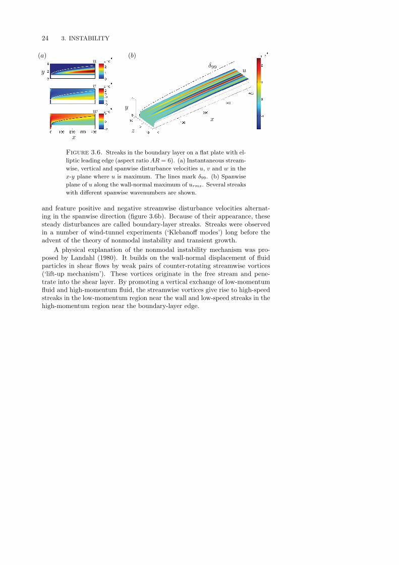
Figure 3.6. Streaks in the boundary layer on a flat plate with el-

liptic leading edge (aspect ratio AR = 6). (a) Instantaneous stream-

wise, vertical and spanwise disturbance velocities u, v and w in the

x-y plane where u is maximum. The lines mark δ99. (b) Spanwise

plane of u along the wall-normal maximum of urms. Several streaks

with different spanwise wavenumbers are shown.

and feature positive and negative streamwise disturbance velocities alternat-ing in the spanwise direction (figure 3.6b). Because of their appearance, thesesteady disturbances are called boundary-layer streaks. Streaks were observedin a number of wind-tunnel experiments (‘Klebanoff modes’) long before theadvent of the theory of nonmodal instability and transient growth.

A physical explanation of the nonmodal instability mechanism was pro-posed by Landahl (1980). It builds on the wall-normal displacement of fluidparticles in shear flows by weak pairs of counter-rotating streamwise vortices(‘lift-up mechanism’). These vortices originate in the free stream and pene-trate into the shear layer. By promoting a vertical exchange of low-momentumfluid and high-momentum fluid, the streamwise vortices give rise to high-speedstreaks in the low-momentum region near the wall and low-speed streaks in thehigh-momentum region near the boundary-layer edge.

CHAPTER 4

Receptivity

Boundary-layer instabilities emerge as a result of a forcing of the layer by itsenvironment1. Sources of such a forcing are, for example, the vortical fluctua-tions of a free stream or the roughness of a wall. If the forced boundary-layerdisturbance is able to feed the eigenmodes of the layer with energy and modalor nonmodal instabilities arise, the layer is said to be receptive to the forcing.

The simplest receptivity mechanism is that of direct receptivity. Direct re-ceptivity requires a resonance between the frequencies and wavenumbers of theenforced disturbances and those of the boundary-layer eigenmodes. A swept-plate boundary layer, for instance, is directly receptive to natural wall rough-ness, because the roughness exhibits a broad range of length scales – amongthem those of the steady crossflow modes. However, many natural free-streamdisturbance sources are not ‘wavenumber resonant’ with the boundary-layermodes. The mismatch in wavenumber arises because the length scales of thefree-stream disturbances are governed by the inviscid dynamics of the outerflow, whereas those of the eigenmodes are determined by the viscous effectsinside the boundary layer. An example is the Blasius boundary layer exposedto a free-stream sound wave at a low Mach number. In the incompressiblelimit, the streamwise wavenumber of the acoustic wave is zero and so is thewavenumber of the disturbance enforced inside the layer (Stokes wave). Thus,the Stokes wave does not directly couple to the large-wavenumber T-S mode ofthe Blasius boundary layer.

Despite the lack of a direct receptivity mechanism, Blasius flow was foundto be receptive to free-stream sound under certain conditions. Goldstein (1983)and Ruban (1985) proposed an explanation for this apparent contradiction byintroducing the concept of length-scale conversion. For the example of Bla-sius flow with free-stream sound, a second – steady – source is required inorder to provide the T-S wavenumber. Therefore, the receptivity mechanismis sometimes called indirect receptivity. Goldstein (1983) demonstrated by anasymptotic analysis that the rapidly developing boundary-layer region near aleading edge can convert the length scale of the enforced Stokes solution intothat of the T-S wave. This is shown in figure 4.1 for the case of free-streamvorticity. Although the free-stream wave exhibits a longer wavelength than theT-S mode, the boundary layer is receptive to the free-stream disturbance. As

1In absolutely unstable flows, the instabilities are sustained without an external forcing (e.g.

Schmid & Henningson 2001).

25

26 4. RECEPTIVITY

Figure 4.1. Excitation by free-stream vorticity of a T-S wave

inside the boundary layer on a plate with an elliptic leading edge.

(a) Streamwise and (b) vertical disturbance velocities.

demonstrated by Goldstein (1985), a streamwise variation in surface geometry,e.g. a roughness bump or a suction hole, can also promote the length-scaleconversion. The asymptotic theory considered by Goldstein (1983, 1985) andRuban (1985) is based on an expansion of the disturbance in powers of 1/Re,which leads to the linearized triple-deck equations. These govern the distur-bance evolution in the limit of high Reynolds numbers. The triple-deck for-mulation is only valid at the first neutral point of the unstable mode (branchI). A successful attempt to extend the receptivity analysis to finite Reynoldsnumbers and to the regions away from the first branch of instability was the fi-nite Reynolds-number theory (FRNT) first proposed by Zavol’skii et al. (1983).The FRNT relies on the same ideas as the classical linear stability theory (see§3.2). These are the assumption of a locally parallel baseflow and the limitationto small disturbance amplitudes, allowing for a linearization of the governingequations. The FRNT was successfully applied to two-dimensional flat-plateflows (Crouch 1992; Choudhari & Streett 1992) and to Falkner-Skan-Cookeboundary layers (Crouch 1993, 1994; Choudhari 1994).

4.1. Receptivity coefficients

During the receptivity phase, the external forcing imposes the upstream ampli-tude (‘initial condition’) of the boundary-layer instabilities at the receptivitysite (e.g. a roughness bump). This amplitude may therefore be called receptiv-ity amplitude (denoted byAR here). It is obvious that the receptivity amplitudedepends on the amplitude ε of the ambient perturbation. If AR is proportionalto ε, the receptivity to the forcing is linear. It is customary to introduce theratio between AR and ε, referred to as receptivity coefficient,

CR =AR

ε. (4.1)

For linear receptivity, CR is constant upon varying the forcing amplitude ε. Theassumption of linear receptivity only holds for ambient perturbations with smallamplitudes. The receptivity of swept-plate flow to shallow localized roughnessbumps is an example for a linear mechanism. For indirect receptivity, i.e. thereceptivity to a combination of two external sources (e.g. coupling of sound at

4.1. RECEPTIVITY COEFFICIENTS 27

roughness), CR is written as

CR =AR

ε1ε2, (4.2)

where ε1 and ε2 are the amplitudes of the two sources. The indirect receptivityis linear if AR is proportional to both ε1 and ε2. There also exist receptivitymechanisms which are nonlinear even for small amplitudes. For example, thereceptivity of boundary layers to pairs of oblique vortical free-stream wavesis quadratic in the amplitude of the free-stream disturbance. The receptivitycoefficient for quadratic receptivity is

CR =AR

ε2. (4.3)

In general, we may summarize (4.1), (4.2) and (4.3) by stating

CR =Initial instability amplitude

Amplitudes of the perturbation sources, (4.4)

i.e. the receptivity coefficient is a measure for the efficiency of the energy trans-fer from the forcing to the boundary-layer instability. The receptivity amplitudeAR and the forcing amplitude ε should be chosen such that they reflect in aproper way the nature of the triggered instability and the characteristics of theforcing. Common choices of AR are the wall-normal maximum of the stream-wise disturbance-velocity amplitude (or the r.m.s.) and quantities based ona wall-normal integration of the disturbance-velocity profiles. The choice of εdepends on the type of disturbance source considered. An example for surfaceroughness is given in §4.2.1.

The receptivity coefficients are key to a receptivity analysis of boundary-layer flows. They can be combined with standard transition-prediction methodsbased on linear stability theory (e.g. the eN -method) in order to provide arefined prediction tool for industrial use, including the receptivity. Since theinstability amplitudes obtained by the eN -method are usually normalized bytheir magnitude at the first neutral instability point, it is more convenient todefine the receptivity coefficients at branch I rather than at the receptivity site.These branch-I coefficients are sometimes referred to as effective coefficients,denoted by Ceff

R here. The effective receptivity coefficients can be used todetermine the disturbance amplitude A(x) at any location in the linear regimedownstream of the receptivity site. If the N -factor of the instability is known,the disturbance amplitude can be written as

A(x) = εCeffR eN(x). (4.5)

Since the receptivity mechanisms depend on a wealth of factors – e.g. the flowconfiguration, the perturbation environment and the nature of the dominantinstabilities – the application of the results from a receptivity analysis in anindustrial context will require a vast database of receptivity coefficients. Thismotivates the continuation of receptivity research in order to develop refinedtheoretical receptivity models. Direct numerical simulations and large-eddy

28 4. RECEPTIVITY

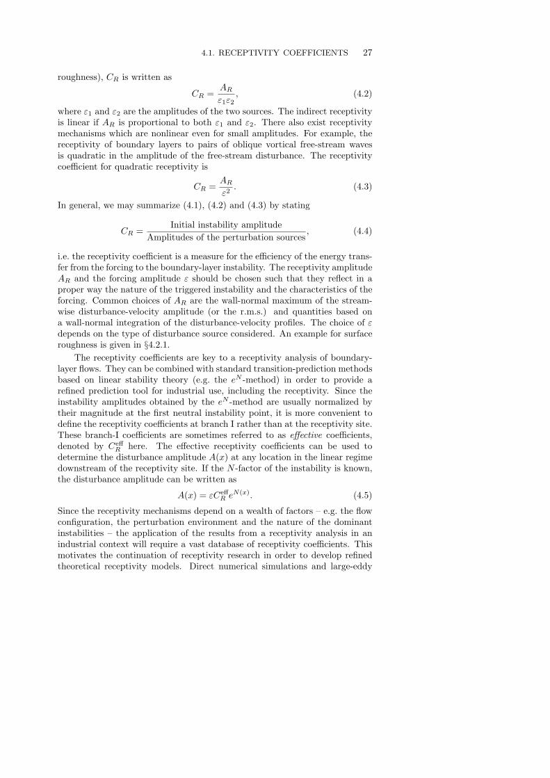
Figure 4.2. Streamwise localized roughness element with span-

wise sinusoidal shape.

simulations like those presented in this thesis will continue to serve as validationtools for these models.

4.2. Examples of boundary-layer receptivity

4.2.1. Direct receptivity of swept-plate flow to roughness

Consider the swept-plate boundary layer depicted in figure 2.3, which is un-stable to crossflow modes (§3.3.1). Steady crossflow vortices can be excited bywall roughness via a direct receptivity mechanism. This receptivity was ex-amined here by considering the roughness element sketched in figure 4.2. Theroughness is localized in the chordwise direction and periodic in the spanwisedirection. Therefore, the bump enforces a steady boundary-layer disturbancewith a large number of chordwise wavenumbers (denoted by α) and one singlespanwise wavenumber (βr). Instead of prescribing the roughness as a deforma-tion of the wall, we modeled it in terms of inhomogeneous boundary conditionsfor the enforced disturbance. These conditions are obtained by a projection ofthe no-slip conditions at the bump contour onto the smooth wall (index ‘0’),using the wall-normal gradient of the baseflow profiles,

u0(x, z) = −h(x)(∂U

∂y

)0

sin (βrz), (4.6)

where h(x) is the chordwise shape of the roughness. After a chordwise Fouriertransformation, the roughness model becomes

u0(α, βr) = −H(α)

(∂U

∂y

)0

sin (βrz), (4.7)

with H(α) being the chordwise wavenumber spectrum of the roughness. Here,the spectrum was manipulated by altering the chordwise bump shape. Thisis seen in figure 4.3(a), where three different bump contours (inset) and their

wavenumber spectra |H| are depicted. We also varied the spanwise wavenumber

4.2. EXAMPLES OF BOUNDARY-LAYER RECEPTIVITY 29

0 0.2 0.4 0.6 0.80

5

10

15

10 20 300

1

(a)

H

αR

x

hx

0.1 0.3 0.5

0.01

0.015

(b)

CR

βR

Figure 4.3. (a) Bumps with three different streamwise shapes in

physical space (inset) and Fourier space. (b) Receptivity coefficients

for roughness elements with different spanwise wavenumbers and

streamwise shapes. The coefficients were extracted from DNS data.

The peak is explained in paper 1. The thin curve pertains to the

receptivity of a streamwise constant (‘parallel’) basic state.

βr of the roughness. The symbols in figure 4.3(a) mark the spectral bump am-

plitudes |H(αCF )| obtained at the wavenumbers αCF of the unstable crossflowmodes pertaining to three values of βr. Figure 4.3(b) shows the receptivity co-efficients obtained. The most remarkable result is that the receptivity becomesindependent of the chordwise bump shape for nearly all spanwise wavenumbersconsidered2. This shape independence is obtained if the amplitude ε of theforcing (cf. §4.1) is defined as ε = εr|H(α)|, where εr is the roughness height.The receptivity coefficient for roughness-induced steady crossflow instability isthen

CR =ACF

εr|H(αCF )|, (4.8)

where ACF is the receptivity amplitude of the excited crossflow vortex at theroughness site. Note that (4.8) can be derived in the FRNT framework when theroughness model (4.7) is used (see e.g. Choudhari 1994, for indirect receptivityto roughness and sound).

4.2.2. Receptivity to vertical vorticity at a leading edge

Figure 4.4 is a close-up of the leading edge region of the flow configurationdepicted in figure 2.7. A steady free-stream vortical disturbance in the form ofa spanwise sinusoidal distribution of the streamwise velocity is considered. Thisparticular disturbance is characterized by a vertical vorticity vector, i.e. thestreamwise and spanwise vorticity components are zero. When the disturbanceimpinges onto the leading edge, a spanwise velocity disturbance (‘crossflow’) isproduced (figure 2.7, plane I). Downstream of the leading edge (plane II), we

2Conditions for which the shape independence becomes invalid are discussed in paper 1.

30 4. RECEPTIVITY

x

y

z

δ99

Plane III

Plane II

Plane I

Figure 4.4. Instantaneous boundary-layer response to a single

free-stream vortical mode with vertical vorticity only. The lead-

ing edge with aspect ratio AR = 6 is considered. Plane I: colors,

spanwise disturbance velocity; vectors, streamwise and spanwise

disturbance. Plane II: vertical disturbance velocity (×5). Plane

III: colors, streamwise disturbance velocity; vectors, vertical and

spanwise components.

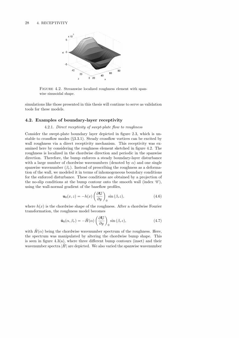
also identify a weak vertical velocity component. The vertical and spanwisedisturbances establish a streamwise vortical motion near the boundary-layeredge. These counter-rotating vortices are able to penetrate into the boundarylayer and produce streamwise disturbance streaks inside the layer (figure 2.7,plane III). The receptivity mechanism to vertical free-stream vorticity at aleading edge is summarized as follows. When impinging on the leading edge, thevertical vorticity is converted into streamwise vorticity via vortex stretching andvortex tilting. The counter-rotating streamwise vortices produce the boundary-layer streaks by the lift-up mechanism (cf. §3.5). Figure 4.5 shows boundary-layer streaks generated by this receptivity mechanism. Two leading edges withdifferent bluntness and various spanwise wavenumbers are considered. Thestreak amplitudes are significantly larger when the leading edge is blunt. Thissuggests that the stretching and tilting of the vertical disturbance vorticity areenhanced at blunt leading edges. We conclude that boundary layers on bluffbodies are more receptive to vertical free-stream vorticity than those on slenderbodies.

4.2. EXAMPLES OF BOUNDARY-LAYER RECEPTIVITY 31

0 50 100 150 2000

4

8

12

|uj |εj

x

β=2.161.44

0.72

2.16

1.44

0.72

Figure 4.5. Downstream development of boundary-layer streaks

with different spanwise wavenumbers. These streaks were initiated

by the receptivity of the leading-edge flow to a free-stream distur-

bance with vertical vorticity only. Downstream of a blunt leading

edge (AR = 6, dashed lines), the streak amplitudes are larger than

downstream of a slender leading edge (AR = 20, solid lines).

4.2.3. Nonlinear receptivity of Gortler flow to free-stream vorticity

For low-amplitude perturbations, the receptivity mechanisms presented in§§4.2.1 and 4.2.2 are linear in the amplitude of the external forcing (rough-ness and vortical mode, respectively). Here, we present a nonlinear receptiv-ity mechanism for a pair of high-frequency oblique vortical modes in the freestream over a concave plate (see §2.3.2). Figure 4.6 shows the response of theGortler boundary layer to this kind of external forcing. A temporal-spanwiseFourier transform reveals that the flow response not only contains componentswith the fundamental frequency and spanwise wavenumber of the forcing, butalso harmonic and subharmonic contributions (figure 4.6a). Downstream, themost energetic component is a zero-frequency disturbance with twice the span-wise wavenumber of the free-stream vorticity. This component is the Gortlerroll shown in figure 3.4 and results from a nonlinear interaction between thefundamental components enforced by the free-stream disturbance. Hence, theGortler boundary layer is receptive to high-frequency free-stream vortices, andthe receptivity mechanism associated with the steady Gortler roll is nonlinearin the forcing amplitude. Figure 4.6(b) shows that the receptivity coefficientof this mechanism (defined in 4.3) decreases with increasing frequency of thefree-stream disturbances.

32 4. RECEPTIVITY

0 300 600 90010

−5

10−3

10−1

ξ

u, u

rms

(F,β)=(F0 ,β0)

(0,2β0)

(0,0)

<

(a)

100 200 300 400200

220

240

260

F

Cv

C of (0,2β )-mode0v

(b)

Figure 4.6. (a) Decomposition of the disturbance enforced in-

side a Gortler boundary layer by a weak pair of oblique vortical

free-stream modes. Contributions with different frequencies and

spanwise wavenumbers versus the tangential plate coordinate ξ. (b)

Coefficient for nonlinear receptivity to oblique free-stream modes

versus frequency of the external forcing.

CHAPTER 5

Breakdown

The final step of laminar-turbulent transition in boundary layers is the break-down to turbulence, which occurs in layers with high-intensity disturbances.The breakdown is preceded by a saturation of the disturbance amplitude, in-dicating a nonlinear redistribution of energy to a broad range of disturbancescales (frequency/wavenumber cascade). This cascade results from nonlinearself-interactions of the fundamental disturbance and from mutual interactionsbetween different disturbance components, promoting the emergence of har-monic and subharmonic modes, respectively. At this stage, the disturbanceenvironment inside the boundary layer is complex, the primary disturbancesin turn become unstable and a new type of instability develops on top of theflow. These new disturbances are referred to as secondary modes in orderto distinguish them from the primary disturbances. It is believed that thesecondary instabilities are excited by high-frequency fluctuations of the flow(e.g. free-stream turbulence). The appearance of the secondary instabilitiesdepends on the type of boundary layer and on the kind of primary distur-bance (e.g. modal/nonmodal). The secondary instabilities have, on the otherhand, in common that they are three-dimensional in nature, appear as small-scale vortical structures and feature large growth rates, thus promoting a rapidbreakdown of the primary instabilities. The breakdown becomes manifest inthe formation of turbulent spots at random locations. These spots are patchesof turbulent motion in a perturbed laminar flow (intermittent state). Since theleading edge of the turbulent spots propagates faster than the trailing edge, thespots grow in size and merge with each other. This leads to a fully turbulentboundary layer downstream.

5.1. Examples of secondary instability and breakdown

5.1.1. Streak instability in flat-plate flows

Figure 5.1 shows quasi-steady low-momentum and high-momentum stream-wise disturbance streaks in a flat-plate boundary layer. These streaks wereextracted from a DNS of zero pressure-gradient flow with a turbulent freestream (cf. Brandt et al. 2004; Schlatter et al. 2008). Upon saturation, thestreaks strongly deform the underlying baseflow, producing inflectional wall-normal and spanwise profiles of the streamwise velocity. At this stage, thelow-speed streaks become susceptive to secondary instabilities, which may be-come manifest in a spanwise meandering of the streaks (figure 5.1a). This type

33

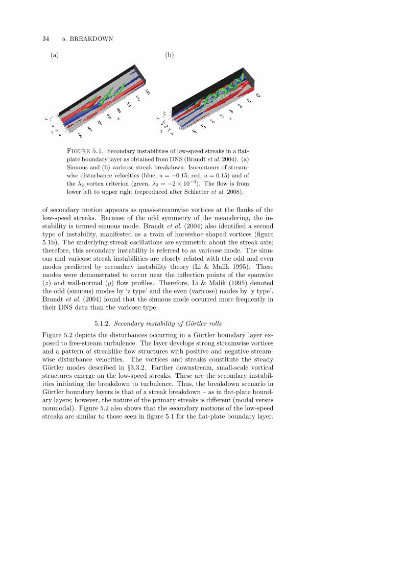
34 5. BREAKDOWNy

z

x

(a)

x

z

y

(b)

Figure 5.1. Secondary instabilities of low-speed streaks in a flat-

plate boundary layer as obtained from DNS (Brandt et al. 2004). (a)

Sinuous and (b) varicose streak breakdown. Isocontours of stream-

wise disturbance velocities (blue, u = −0.15; red, u = 0.15) and of

the λ2 vortex criterion (green, λ2 = −2 × 10−3). The flow is from

lower left to upper right (reproduced after Schlatter et al. 2008).

of secondary motion appears as quasi-streamwise vortices at the flanks of thelow-speed streaks. Because of the odd symmetry of the meandering, the in-stability is termed sinuous mode. Brandt et al. (2004) also identified a secondtype of instability, manifested as a train of horseshoe-shaped vortices (figure5.1b). The underlying streak oscillations are symmetric about the streak axis;therefore, this secondary instability is referred to as varicose mode. The sinu-ous and varicose streak instabilities are closely related with the odd and evenmodes predicted by secondary instability theory (Li & Malik 1995). Thesemodes were demonstrated to occur near the inflection points of the spanwise(z) and wall-normal (y) flow profiles. Therefore, Li & Malik (1995) denotedthe odd (sinuous) modes by ‘z type’ and the even (varicose) modes by ‘y type’.Brandt et al. (2004) found that the sinuous mode occurred more frequently intheir DNS data than the varicose type.

5.1.2. Secondary instability of Gortler rolls

Figure 5.2 depicts the disturbances occurring in a Gortler boundary layer ex-posed to free-stream turbulence. The layer develops strong streamwise vorticesand a pattern of streaklike flow structures with positive and negative stream-wise disturbance velocities. The vortices and streaks constitute the steadyGortler modes described in §3.3.2. Farther downstream, small-scale vorticalstructures emerge on the low-speed streaks. These are the secondary instabil-ities initiating the breakdown to turbulence. Thus, the breakdown scenario inGortler boundary layers is that of a streak breakdown – as in flat-plate bound-ary layers; however, the nature of the primary streaks is different (modal versusnonmodal). Figure 5.2 also shows that the secondary motions of the low-speedstreaks are similar to those seen in figure 5.1 for the flat-plate boundary layer.

5.1. EXAMPLES OF SECONDARY INSTABILITY AND BREAKDOWN 35

Figure 5.2. Disturbance structures in the transitional region of

a Gortler boundary layer subject to free-stream turbulence (from

DNS). Isosurfaces of streamwise disturbance velocities (blue, u =

−0.25; red, u = 0.2) and of the λ2 vortex-identification criterion

(green, λ2 = −5× 10−4). The flow is from left to right.

In particular, a distinct horseshoe-vortex train is prominent in figure 5.2, indi-cating a varicose streak breakdown. The low-speed streak at z = 30, in contrast,features the spanwise meandering due to quasi-streamwise vortices typical ofa sinuous secondary instability. The downstream region of the boundary layeris characterized by spanwise alternating patches of laminar and turbulent flow(intermittency), which highlights the local nature of the breakdown to turbu-lence.

5.1.3. Turbulent spots in swept-plate flows

We now consider the swept-plate boundary layer described in §2.3.1. Figure5.3 depicts the boundary-layer disturbance structures excited by free-streamturbulence. The primary disturbances consist of traveling crossflow waveswith different frequencies, spanwise wavelengths and amplitudes (‘wave pack-ets’). After saturating, these waves become susceptive to secondary instabilitymodes. Malik et al. (1999) performed a secondary instability analysis of sat-urated crossflow vortices and identified ‘z modes’ and ‘y modes’ in analogy tothose discussed in §5.1.1. Wassermann & Kloker (2003) investigated in detailthe secondary instabilities of traveling crossflow waves, using DNS. The mostunstable secondary mode was found near the wall and corresponded to the ‘z

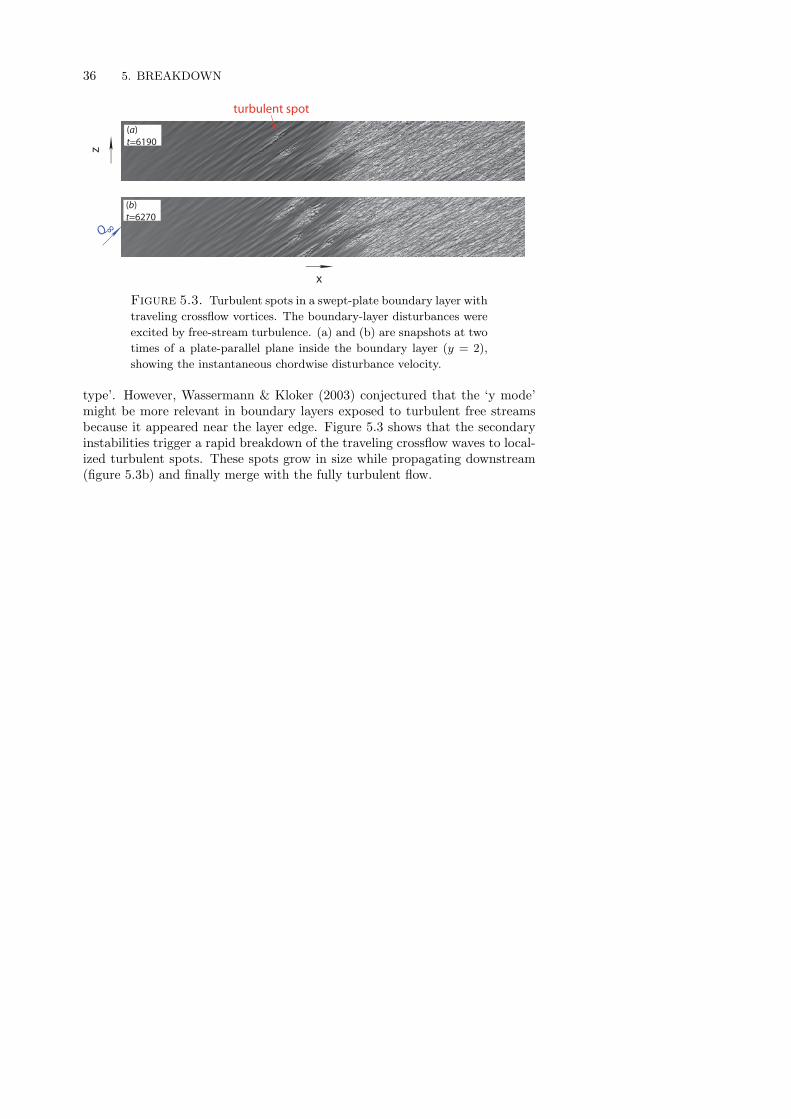
36 5. BREAKDOWN

(a)

t=6190

(b)

t=6270

x

z

Q8

turbulent spot

Figure 5.3. Turbulent spots in a swept-plate boundary layer with

traveling crossflow vortices. The boundary-layer disturbances were

excited by free-stream turbulence. (a) and (b) are snapshots at two

times of a plate-parallel plane inside the boundary layer (y = 2),

showing the instantaneous chordwise disturbance velocity.

type’. However, Wassermann & Kloker (2003) conjectured that the ‘y mode’might be more relevant in boundary layers exposed to turbulent free streamsbecause it appeared near the layer edge. Figure 5.3 shows that the secondaryinstabilities trigger a rapid breakdown of the traveling crossflow waves to local-ized turbulent spots. These spots grow in size while propagating downstream(figure 5.3b) and finally merge with the fully turbulent flow.

CHAPTER 6

Numerical methods

6.1. Direct numerical simulation

Most results presented in this thesis were obtained by spatial direct numeri-cal simulations (DNS). DNS is a numerical technique, by which the governingequations are solved directly. Terms of the Navier-Stokes equations are neitheromitted (as in the PSE) nor modeled (as in the RANS equations). However,some modeling is introduced in the DNS framework by the treatment of theboundaries. These boundaries arise due to a truncation of the flow domain. Anexample is the modeling of (statistically) spanwise invariant flows by periodicboundary conditions. The assumption of periodicity at the spanwise bound-aries introduces a fundamental spanwise wavelength (the width of the domain),which must be chosen such that it does not interfere with the physically relevantlength scales of the flow.

The DNS approach requires a resolution of all dynamically important flowstructures. This is an easy task for a low Reynolds-number laminar bound-ary layer. However, since the ratio between the largest and the smallest flowstructures is proportional to Re3/4 (length-scale cascade), the spatial resolutiondemands for a three-dimensional DNS increase as Re9/4 (Moin & Kim 1997)1.Moreover, an increase in spatial resolution requires – for methods with explicittime advancement – a reduction of the time step in order not to violate the CFLcondition of numerical stability. Kim et al. (1987) and Spalart (1988) give rec-ommendations for the maximum allowed grid spacings for DNS of wall-boundedturbulent flows. These are ∆x+ = 15, ∆y+ = 1 at the wall and ∆z+ = 8 inthe streamwise, vertical and spanwise directions, respectively. The symbol ‘+’denotes a normalization by ν/uτ (‘wall units’), where uτ =

√τw/ρ is the fric-

tion velocity. Most simulations reported in this thesis consider pre-transitionallaminar boundary layers, characterized by larger flow structures than those inturbulent layers. The grid spacings of these DNS can therefore be chosen largerthan the values given above2. On the other hand, we also present simulationsof transition to turbulence in a swept-plate boundary layer. In the chordwise

1This scaling holds for DNS of homogeneous isotropic turbulence. The increase in grid points

is usually less for DNS of boundary layers, because only the resolution of the layer – but notthat of the free stream – needs to be refined.2This holds, in particular, for DNS of linear receptivity and instability by a spectral method

for the solution of the linearized Navier-Stokes equations, allowing for a significant reductionof the spanwise resolution.

37

38 6. NUMERICAL METHODS

and spanwise directions, the grid spacings of these simulations fulfilled the rec-ommendations cited above, whereas the smallest wall-normal grid spacing wassomewhat larger than ∆y+ = 1. Therefore, while being small enough to cap-ture the flow structures in the pre-transitional boundary layer, the vertical gridspacing was insufficient in order to resolve the smallest scales of the fully turbu-lent flow. This lack of resolution was compensated for by using an LES subgridmodel. The model mimicked the influence of the unresolved fluctuations onthe smallest turbulent motions resolved, while being inactive in the laminarregion of the boundary layer. This example shows that simulations may beconsidered DNS in certain regions of the flow field, whereas other regions areunder-resolved, requiring a model.

We summarize that the DNS technique allows for high-fidelity simulationsincluding all relevant length and time scales of a flow. On the other hand, theprice to pay is that of long simulation times. In recent years, DNS has be-come more affordable thanks to the advent of supercomputers and parallelizedsimulation codes.

6.2. Simulation codes

The results in this thesis were obtained by using the simulation codes Simsonand Nek5000. Simson uses a global spectral method (GSM) and is documentedin Chevalier et al. (2007). The time-dependent incompressible Navier-Stokesequations are implemented in the velocity-vorticity formulation, where the wall-normal components of the velocity and the vorticity are the dependent flow vari-ables. The wall-parallel velocity components are retrieved using the continuityequation and the definition of wall-normal vorticity. The spatial discretizationof the governing equations builds on Fourier expansions in the wall-paralleldirections and a Chebyshev expansion in the wall-normal direction. The useof Chebyshev polynomials is beneficial for simulations of wall-bounded flows,because the associated weight functions naturally concentrate the wall-normalresolution towards the wall. The use of Fourier modes requires spatially pe-riodic solutions. Periodicity can often be assumed in the spanwise direction(spanwise invariant flows); however, boundary-layer flows are not streamwiseinvariant. The required streamwise periodicity must be artificially imposed bya ‘fringe region’ at the downstream end of the computational domain, in whichthe flow is forced towards the inflow conditions (Bertolotti et al. 1992)3.

The terms of the governing equations are evaluated in Fourier-Chebyshevspectral space except for the nonlinear terms, which are computed in physicalspace (‘pseudo-spectral’ treatment). This involves products between expansioncoefficients, with the products at highest order (N , say) effectively leading toan expansion up to order 2N . If the number of collocation points is only equalto N , the numerical quadrature is not exact and introduces aliasing errors. Forincompressible flows, these can be removed by using ≥ 3N/2 collocation points(3/2-rule, Spalart et al. 1991). The time advancement of Simson is based on

3See also paper 1

6.2. SIMULATION CODES 39

a combined implicit-explicit scheme. The linear terms of the Navier-Stokesequations are discretized in time by a second-order implicit Crank-Nicolsonscheme, whereas the nonlinear terms are discretized explicitly, using a third-order four-step Runge-Kutta scheme.

The global nature of the GSM becomes manifest in the use of globalbasis functions in the expansions, i.e. these functions are defined on theentire numerical domain. The major benefit of the GSM is the exponentialconvergence of the approximated solution, as the number of grid nodes isincreased. The major shortcoming is the inability to deal with complex flowgeometries and discontinuities of the flow field, e.g. shock waves.

Nek5000 is an implementation of the spectral element method (SEM) by Patera(1984) and is documented in (see Tufo & Fischer 1999; Fischer et al. 2008). Theflow domain is decomposed into spectral elements, which in turn are subdividedby arrays of spectral interpolation nodes. Thus, the decomposition is both ina spatial and a spectral sense. Therefore, the SEM is sometimes classified as amethod in between finite element methods and global spectral methods. TheSEM is based on the weak statement of the incompressible Navier-Stokes equa-tions, obtained by multiplying the terms of the equations by test functions andintegrating over the physical domain. In particular, the viscous terms are inte-grated by parts, which leads to a reduction of the order of the derivatives in theviscous terms from two to one. The spatial discretization uses a Galerkin pro-jection onto a subspace spanned by orthogonal polynomial functions. These areLagrangian interpolants defined on Gauss-Lobatto-Legendre (GLL) nodes forthe velocity space and Gauss-Legendre (GL) nodes for the pressure space, usingLegendre polynomials. The interpolation is performed on GLL/GL reference el-ements; therefore, the linear combination of the basis functions must be mappedonto the actual elements of the flow domain in order to retrieve the expansionsfor the velocity and the pressure. The use of different subspaces for the velocityand the pressure is similar to the strategy of staggered grids in finite differenceand finite volume methods. The aim is to avoid spurious pressure fluctuations.In Nek5000, the so-called PN -PN−2 discretization by Maday & Patera (1989) isused. As indicated by this notation, the highest order of the polynomials usedfor the pressure expansion is by two lower than that for the velocity expan-sions. As in the GSM, the evaluation of the nonlinear terms leads to aliasingerrors. These are removed by ‘over-integration’ similar to the 3/2-rule of fullyspectral methods. Moreover, a filtering technique is implemented in Nek5000

(Fischer & Mullen 2001), allowing for a damping of the highest-order modesincluded in the expansions. The filtering procedure was developed in order toensure numerical stability for simulations of high-Reynolds number turbulentflows. The discretization in time follows the implicit-explicit operator-splittingmethod by Maday et al. (1990). The viscous terms are treated implicitly, us-ing a third-order backward-difference scheme, while the nonlinear terms arediscretized explicitly by a second-order extrapolation.

40 6. NUMERICAL METHODS

The local nature of the SEM is manifested by the spatial decompositioninto spectral elements. This allows – together with the spectral intra-elementaldiscretization – for two refinement strategies, based on decreasing the size of theelements (‘h refinement’) and on raising the highest order of the polynomialsincluded in the expansions (‘p refinement’). The major benefit of the SEM arisesfrom its local nature, allowing for its application to flows of complex geometry;the major shortcoming is the large computational cost. In order to compensatefor this, Nek5000 was designed for an efficient use on supercomputers withthousands of processors (Tufo & Fischer 2001).

6.3. Comparison

Table 6.1 gives a comparison between the GSM code Simson and the SEM codeNek5000 in order to highlight their applicability and limitations. We summa-rize that the GSM is – due to its efficiency – the preferred tool whenever thegeometry of the simulation domain can be kept simple, allowing for a represen-tation of the flow field in terms of a linear combination of Fourier modes. Forcomplex geometries or flow fields with local steep gradients, requiring local-ized refinement, the SEM is an accurate alternative to finite difference or finitevolume methods. Also note that the SEM passes into a GSM, if the physicaldomain of interest is decomposed into one single element only.

6.3. COMPARISON 41

Table 6.1. Global spectral method (GSM) versus spectral ele-

ment method (SEM).

GSM SEM

Simulationcode

Simson Nek5000

Programminglanguage

Mainly Fortran77 Mainly Fortran77

General Global approach Local approachcharacteristics Fourier-Galerkin-

Chebyshev tau methodGalerkin method

Fast Fourier transformsSpecial fea-tures

Fringe technique

Numericalgrid

Equidistant in the hori-zontal directions, Gauss-Lobatto-Chebyshev nodesin the vertical direction

Sub-domains (spectralelements) with arbi-trary shape, Gauss-Lobatto/Gauss-Lobatto-Legendre points, staggeredgrids

Basis func-tions/ spatialdiscretization

Fourier modes in the hor-izontal directions, Cheby-shev polynomials in the ver-tical direction

Polynomial interpolation ofLagrange form at Legendrenodes

De-aliasing 3/2-rule in the horizontal di-rections

Filtering at the high-est wavenumbers, over-integration

Time integra-tion

Implicit/explicit split-ting: Four-step third orderRunge- Kutta method+ second-order Crank-Nicolson

Implicit/explicit splittingtechnique: Third-orderbackward differentiation+ third-order Adams-Bashforth

Parallelisation MPI and OpenMP MPIPartitioning into slices inthe spanwise direction

Element-wise partitioning

Applications Incompressible laminar andturbulent flows: Channelflow, 2D and 3D boundary-layer flows on flat plates

Massively parallelized sim-ulations of incompressiblelaminar and turbulent flowsin complex geometries

Limitations To problems which can bemade periodic using thefringe technique

Less efficient than the globalspectral method

Simple geometries, e.g. nocurved walls or leading edge

CHAPTER 7

Summary and outlook

The present thesis reports results on the receptivity and instability of spatiallyevolving boundary layers to wall roughness and free-stream vortices. The re-sults have been obtained by direct numerical simulations (DNS), using twodifferent spectral methods. Various boundary-layer flows are considered; theseare a three-dimensional boundary layer of Falkner-Skan-Cooke type, a Gortlerboundary layer, a two-dimensional boundary-layer flow past a flat plate with el-liptic leading edge and a swept-wing boundary layer. These flows accommodatevarious characteristics of the flows over straight and swept wings and bladessuch as the stagnation and attachment at the leading edge, wall curvature,chordwise pressure gradients, streamline curvature and crossflow.

The focus is on the receptivity of these boundary layers. The receptivitydescribes the coupling between the boundary-layer instabilities and the pertur-bations from the surroundings of the boundary layer. A receptivity analysisexplains, by which mechanisms boundary-layer disturbances are produced andhow large the initial amplitudes of these disturbances are. The boundary-layer receptivity must be considered in order to predict the transition locationin boundary layers. Different receptivity mechanisms such as direct and in-direct receptivity and linear and nonlinear receptivity are herein discussed.These mechanisms are characterized in terms of receptivity coefficients, whichare a measure for the coupling efficiency between ambient perturbations andboundary-layer instabilities. Once these receptivity coefficients are known, thestreamwise evolution of the amplitudes of the boundary-layer instabilities canbe predicted, using linear or nonlinear methods (e.g. the PSE method).

The present thesis also reports the linear and nonlinear phases of instabilitygrowth and the breakdown to turbulence. The spatial DNS presented hereare ideally suited in order to identify the relevant flow structures in spatiallydeveloping boundary layers. The value of data from spectral DNS lies in theaccuracy and the completeness of the results; the drawback, on the other hand,is the tremendous computational cost. To date, DNS cannot be used to producehuge databases of receptivity coefficients for different flow parameters of interestfor aeronautical engineers (e.g. Reynolds number or Mach number). Instead,simplified and more efficient methods such as the PSE and the FRNT must beaddressed. These methods must, however, be verified and validated with thehelp of experiments or DNS. A successful validation of the PSE is, for instance,presented in Hogberg & Henningson (1998) and Tempelmann et al. (2010).

42

7. SUMMARY AND OUTLOOK 43

In the near future, the study of swept-wing flows will be extended in orderto determine the receptivity of the wing boundary layer to vortical free-streammodes and free-stream turbulence. We will also consider different representa-tions of surface roughness (both meshed and modeled) and compute the asso-ciated receptivity coefficients. In particular, we will identify the performanceof the standard linear roughness model based on inhomogeneous disturbanceboundary conditions by a comparison with the results for a meshed roughnesselement. PSE calculations will also be considered. The aim is to combine theDNS and the PSE methods by prescribing mean-flow and disturbance profilesobtained by DNS as the upstream (‘initial’) condition for the PSE marchingprocedure. DNS is thus only used where needed (e.g. in the leading-edge re-gion), and the PSE is employed to computed the downstream evolution of thedisturbance input from the DNS.

In the far future, the optimization and flow-control techniques developedat KTH Mechanics will be applied to some of the flow configurations discussedin this thesis. Optimization techniques in hydrodynamics aim to identify theupstream flow structures causing the largest downstream disturbance ampli-tudes inside the boundary layer (‘worst-case scenario’). These techniques havebeen successfully applied to relatively simple flows such as the Blasius bound-ary layer (Monokrousos et al. 2010a) and the Falkner-Skan-Cooke boundarylayer (Tempelmann et al. 2010). Research is currently underway in order toextend the optimization analysis to the flat plate with an elliptic leading edgepresented in this thesis.

The objective of flow control is to manipulate the flow by passive or ac-tive methods such that a certain objective (e.g. the delay of transition or theenhancement of mixing) is achieved. This is, for instance, accomplished byinserting actuators into the boundary layer (e.g. suction holes or active dim-ples). Flow-control techniques devise optimal strategies in order to achievethe objective chosen with the least possible amount of energy for the oper-ation of the actuators. The concepts of flow control were demonstrated intwo-dimensional Blasius flow (Bagheri et al. 2009), and they were recently ex-tended to a three-dimensional configuration of the flat-plate boundary layer(Semeraro et al. 2010). These methods still await their application, for ex-ample, to the swept-wing flow considered in this thesis in order to control theamplitudes of more complicated instabilities such as crossflow vortices. Finally,the concepts of flow control need to be tested by wind-tunnel and in-flight ex-periments. A comparison between experimental and numerical results on flowcontrol in a flat-plate boundary layer is given by Monokrousos et al. (2010b).A setup for wind-tunnel experiments in swept boundary layers is available atKTH Mechanics (Kurian 2010) and may be used for experimental flow controlof crossflow vortices.

Acknowledgements

The present thesis reflects the outcome of about four and a half years of re-search within the VR1 project ‘Receptivity’. Moreover, it also reflects my – theauthor’s – personal development throughout these years at KTH Mechanics.Both my research and personal progress were strongly influenced by my super-visors, Luca Brandt and Dan Henningson.

Luca, although you acted for the first time as a principle PhD supervisor, youguided me through my studies in the best possible manner. I was fortunateto have you as my boss and advisor. Your vast knowledge and experience arecertainly impressive, but your way of dealing with students, of encouragingthem, impressed me even more. Your recipe is your sense of humor. To learnfrom you and work with you was enjoyable.

Dan, although I had quit another PhD project before, you accepted me asyour student – I am grateful for the confidence you had in me. During ourbiweekly research meetings, I learnt a lot from you. Your generosity shall alsobe highlighted here: You gave me the opportunity of attending a number ofconferences, workshops and training courses within the Linne Flow Centre. Ihighly benefited from all these experiences.

Key to my well-being at KTH Mechanics were my wonderful colleagues – cre-ators of an enjoyable working atmosphere. All of you were helpful, open-mindedand behaved like true friends2. Here, I shall devote a one-liner to those of youwho were my longtime fellows and companions:

Shervin – the brilliant. My valued office mate of four and a half years. Es-pen – the social. Although you left the department two years ago, you are stillconstantly cited. Antonios – the charmer. The master of conversation, theowner of charisma and of the secret of coffee brewing. David – the perfect. Theone I discussed most with and learnt most from (apart from my supervisors).Qiang – the modest. You were often able to surprise me with an unexpectedjoke. Johan (Ohlsson) – the rare3. You taught me how to deal with Nek5000

and the Swedes. Johan (Malm) – the busy. “You have a lot of work to do”4.

1Vetenskapsradet – The Swedish Research Council2As opposed to Facebook friends3The only true Swede of our PhD group, potentially with Viking blood4Bogus lawski, L. 2010 Public communication. EFMC-8, Bad Reichenhall, Germany

44

ACKNOWLEDGEMENTS 45

You will manage. Onofrio – the aesthete. The connoisseur of classic music andowner of a fine taste. Lailai – the efficient. I enjoyed your jokes – did youlike mine? Philipp – the instructive. Is there anyone giving more comprehen-sible seminars than you? Yohann – the maıtre du savoir-vivre. The master ofcombining outstanding research with a sense of humor, music, food and wine.Milos – the eloquent. If there is anything to explain, you will find the mostappropriate words to explain it. Ardeshir – the hilarious. Laughing is healthy,you are healthier.

I also want to thank my former colleagues – those who left soon after myarrival and those who only stayed for a short while. These are Astrid, Ori,Olaf, Mathias, Jerome, Martin, Carl-Gustav and Robin5. Good luck to ourfreshmen, Sasan and Reza. Thanks to Subir and Tobias, the two MSc studentsI was in charge of together with Luca. Catherine Mavriplis is acknowledged forher help with Nek5000. The people from the other KTH Mechanics groups notto be forgotten are Andreas, Amin, Enrico, Andreas, Zeinab, Florian, Peter,Tobias and Geert. I shall also thank the staff of the lab at Teknikringen 8, mostnotably Thomas, Bengt, Outi, Ramis, Gabriele, Jens, Fredrik, Nils and Henrik.I am also grateful to the non-academics at KTH Mechanics, in particular toNina, Carolina, Heide, Bubba and Par.

In 2009, I spent six months in Tamer Zaki’s research group at Imperial College,London. I am indebted to Tamer, the master of efficiency and multitasking,who shared his knowledge and experience with me. I shall not forget to thankSandeep, my best friend in London. I made extensive use of your DVAMOstrategy6.

This thesis was proofread by Fredrik Lundell, David Tempelmann and OnofrioSemeraro, who gave valuable hints for its improvement.

Finally, the Swedish taxpayers are acknowledged. The research project wasfunded by VR. The simulations were carried out using SNIC computing fa-cilities at PDC (KTH Stockholm), NSC (Linkopings universitet) and HPC2N(Umea universitet). Moreover, resources of ICT (Imperial College London)were used for parts of the computations.

5Possibly the last KTH Mechanics thesis for you to be acknowledged6Declare Victory And Move On

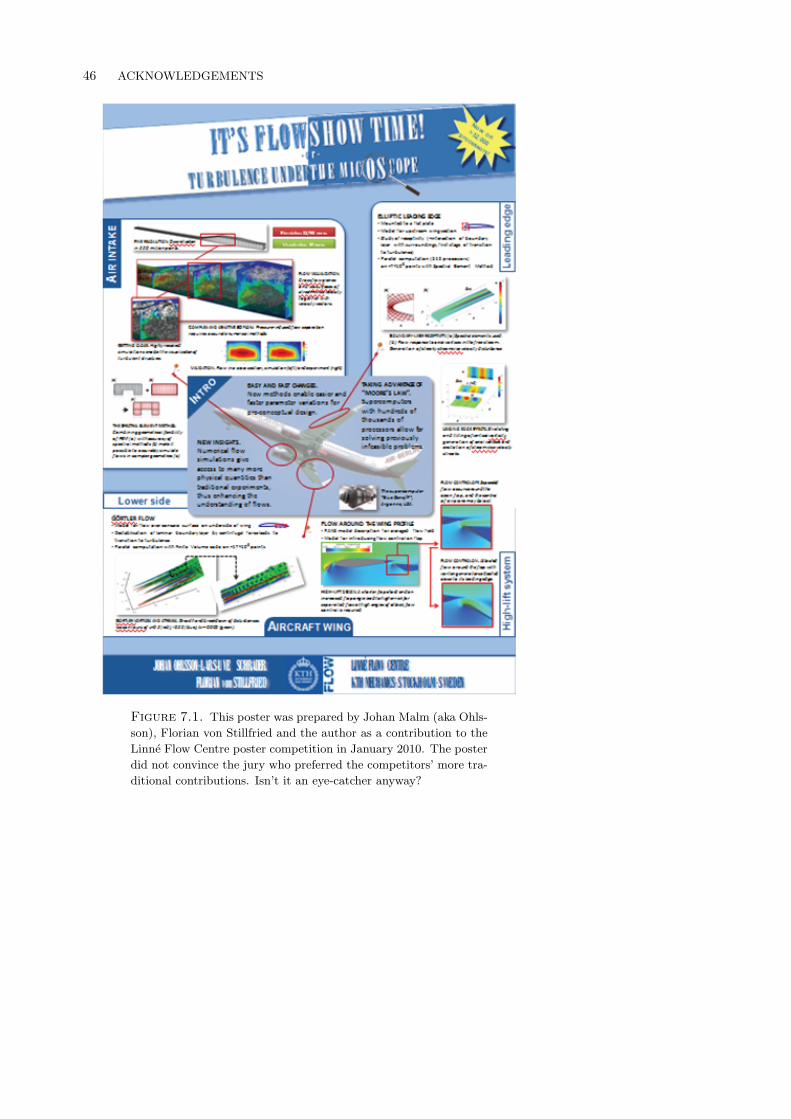
46 ACKNOWLEDGEMENTS

Figure 7.1. This poster was prepared by Johan Malm (aka Ohls-

son), Florian von Stillfried and the author as a contribution to the

Linne Flow Centre poster competition in January 2010. The poster

did not convince the jury who preferred the competitors’ more tra-

ditional contributions. Isn’t it an eye-catcher anyway?

Bibliography

Bagheri, S., Brandt, L. & Henningson, D. S. 2009 Input-output analysis, modelreduction and control of the flat-plate boundary layer. J. Fluid Mech. 620, 263–298.

Bertolotti, F. P., Herbert, T. & Spalart, P. R. 1992 Linear and nonlinearstability of the Blasius boundary layer. J. Fluid Mech. 242, 441–474.

Brandt, L., Schlatter, P. & Henningson, D. S. 2004 Transition in boundarylayers subject to free-stream turbulence. J. Fluid Mech. 517, 167–198.

Butler, K. M. & Farrell, B. F. 1992 Three-dimensional optimal perturbations inviscous shear flow. Phys. Fluids A 4, 1637–1650.

Chevalier, M., Schlatter, P., Lundbladh, A. & Henningson, D. S. 2007 APseudo-Spectral Solver for Incompressible Boundary Layer Flows. Tech. RepTRITA-MEK 2007:07. Royal Institute of Technology (KTH), Dept. of Mechanics,Stockholm.

Choudhari, M. 1994 Roughness-induced Generation of Crossflow Vortices in Three-Dimensional Boundary Layers. Theoret. Comput. Fluid Dynamics 6, 1–30.

Choudhari, M. & Streett, C. L. 1992 A finite Reynolds number approach for theprediction of boundary layer receptivity in localized regions. Phys. Fluids A 4,2495–2514.

Cooke, J. C. 1950 The boundary layer of a class of infinite yawed cylinders. In Proc.Camb. Phil. Soc., , vol. 46, pp. 645–648.

Crouch, J. D. 1992 Localized receptivity of boundary layers. Phys. Fluids A 4 (7),1408–1414.

Crouch, J. D. 1993 Receptivity of three-dimensional boundary layers. AIAA Pa-per (93-0074).

Crouch, J. D. 1994 Distributed excitation of Tollmien-Schlichting waves by vorticalfree-stream disturbances. Phys. Fluids 6 (1), 217–223.

Ellingsen, T. & Palm, E. 1975 Stability of linear flow. Phys. Fluids 18, 487–488.

Falkner, V. M. & Skan, S. W. 1931 Solutions of the boundary layer equation 12,865–896.

Fischer, P., Kruse, J., Mullen, J., Tufo, H., Lottes, J. & Kerke-meier, S. 2008 NEK5000 - Open Source Spectral Element CFD solver .Https://nek5000.mcs.anl.gov/index.php/MainPage.

Fischer, P. F. & Mullen, J. 2001 Filter-based stabilization of spectral elementmethods. C. R. Acad. Sci. Paris t. 332, Serie I, 265–270.

47

48 BIBLIOGRAPHY

Fjørtoft, R. 1950 Application of integral theorems in deriving criteria of instabilityfor laminar flows and for the baroclinic circular vortex. Geofys. Publ., Oslo 17(6), 1–52.

Floryan, J. M. & Saric, W. S. 1982 Stability of Gortler vortices in boundarylayers. AIAA Journal 20 (3), 316–324.

Goldstein, M. E. 1983 The evolution of Tollmien-Schlichting waves near a leadingedge. J. Fluid Mech. 127, 59–81.

Goldstein, M. E. 1985 Scattering of acoustic waves into Tollmien-Schlichting wavesby small streamwise variations in surface geometry. J. Fluid Mech. 154, 509–529.

Gortler, H. 1941 Instabilitat laminarer Grenzschichten an konkaven Wandengegenuber gewissen dreidimensionalen Storungen. ZAMM 21, 250–252, in Ger-man.

Hall, P. 1983 The linear development of Gortler vortices in growing boundary layers.J. Fluid Mech. 130, 41–58.

Henningson, D. S. & Akervik, E. 2008 The use of global modes to understandtransition and perform flow control. Phys. Fluids 20 (031302).

Herbert, T. 1997 Parabolized stability equations. Annu. Rev. Fluid Mech. 29, 245–283.

Herbert, T. & Bertolotti, F. P. 1987 Stability analysis of nonparallel boundarylayers. Bull. Am. Phys. Soc. 32, 2079.

Hogberg, M. & Henningson, D. S. 1998 Secondary instability of cross-flow vorticesin Falkner-Skan-Cooke boundary layers. J. Fluid Mech. 368, 339–357.

Hultgren, L. S. & Gustavsson, L. H. 1981 Algebraic growth of disturbances in alaminar boundary layer. Phys. Fluids 24, 1000–1004.

Kim, J., Moin, P. & Moser, R. D. 1987 Turbulence statistics in fully developedchannel flow at low Reynolds number. J. Fluid Mech. 177, 133–166.

Klebanoff, P. S. 1971 Effect of free-stream turbulence on the laminar boundarylayer. Bull. Am. Phys. Soc. 10, 1323.

Kurian, T. 2010 An experimental investigation of disturbance growth in boundarylayer flows. Tech. Rep TRITA-MEK 2010:04. KTH Royal Institute of Technology,Department of Mechanics, Linne Flow Centre, Stockholm, Sweden.

Landahl, M. T. 1980 A note on an algebraic instability of inviscid parallel shearflows. J. Fluid Mech. 98, part 2, 243–251.

Li, F. & Malik, M. R. 1995 Fundamental and subharmonic secondary instabilitiesof Gortler vortices. J. Fluid Mech. 297, 77–100.

Lin, C. C. 1955 The Theory of Hydrodynamic Stability . Cambridge University Press.

Lin, N., Reed, H. & Saric, W. 1992 Effect of leading edge geometry on boundary-layer receptivity to freestream sound. In Instability, Transition and Turbulence(ed. M. Hussaini, A. Kumar & C. Streett). Springer.

Mack, C. J., Schmid, P. J. & Sesterhenn, J. L. 2008 Global stability of sweptflow around a parabolic body: connecting attachment-line and crossflow modes.J. Fluid. Mech. 611, 205–214.

Maday, Y. & Patera, A. T. 1989 Spectral element methods for the Navier-Stokesequations. In State of the Art Surveys in Computational Mechanics (ed. A. K.Noor), pp. 71–143. ASME, New York.

Maday, Y., Patera, A. T. & Ronquist, E. M. 1990 An operator-integration-factor

BIBLIOGRAPHY 49

splitting method for time-dependent problems: Application to incompressiblefluid flow. J. Sci. Comput. 5(4), 310–337.

Malik, M. R., Li, F., Choudhari, M. M. & Chang, C.-L. 1999 Secondary insta-bility of crossflow vortices and swept-wing boundary-layer transition. J. FluidMech. 399, 85–115.

Moin, P. & Kim, J. 1997 Tackling Turbulence with Supercomputers. Sci. Americanpp. 62–68.

Monokrousos, A., Akervik, E., Brandt, L. & Henningson, D. S. 2010a Globaloptimal disturbances in the blasius boundary-layer flow using time-steppers.J. Fluid Mech. 650, 181–214.

Monokrousos, A., Lundell, F. & Brandt, L. 2010b Feedback control of boundarylayer bypass transition: Comparison of a numerical study with experiments.AIAA Journal 48 (8), 1848–1851.

Orr, W. M. F. 1907 The stability or instability of the steady motions of a perfectliquid and of a viscous liquid. Part I: A perfect liquid. Part II: A viscous liquid.In Proc. Roy. Irish Acad. A, , vol. 27, pp. 9–138.

Patera, A. T. 1984 A Spectral Element Method for Fluid Dynamics: Laminar Flowin a Channel Expansion. J. Comp. Phys. 54, 468–488.

Prandtl, L. 1905 Uber Flussigkeitsbewegung bei sehr kleiner Reibung. In Verhand-lungen des dritten internationalen Mathematiker-Kongresses in Heidelberg 1904(ed. A. Krazer), pp. 484–491. Teubner, Leipzig.

Rayleigh, J. W. S. 1880 On the stability, or instability, of certain fluid motions.Proc. Lond. Math. Soc. 11, 57–70.

Rayleigh, J. W. S. 1916 On the dynamics of revolving fluids. Proc. Roy. Soc. Lond.A 93, 148–154.

Reddy, S. C. & Henningson, D. S. 1993 Energy growth in viscous channel flows.J. Fluid Mech. 252, 209–238.

Reynolds, O. 1883 On the experimental investigation of the circumstances whichdetermine whether the motion of water shall be direct or sinuous, and the law ofresistance in parallel channels. Phil. Trans. R. Soc. Lond. Mech. 174, 935–982.

Ruban, A. I. 1985 On the generation of Tollmien-Schlichting waves by sound.Fluid Dynamics 19, 709–716, translated from Izvestiya Akademii Nauk SSSR,Mekhanika Zhidkosti i Gaza, No. 5, pp. 44–52, 1984.

Saric, W. S. 1994 Gortler vortices. Annu. Rev. Fluid Mech. 26, 379–409.

Schlatter, P., Brandt, L., deLange, H. C. & Henningson, D. S. 2008 Onstreak breakdown in bypass transition. Phys. Fluids 20 (101505), invited paper.

Schmid, P. J. & Henningson, D. S. 2001 Stability and Transition in Shear Flows.Springer.

Schubauer, G. B. & Skramstad, H. K. 1947 Laminar boundary layer oscillationsand stability of laminar flow. J. Aero. Sci. 14, 69–78.

Semeraro, O., Bagheri, S., Brandt, L. & Henningson, D. S. 2010 Feedbackcontrol of three-dimensional optimal disturbances using reduced-order models.J. Fluid Mech. Submitted.

Somers, D. M. & Horstmann, K.-H. 1985 Design of a Medium-Speed, Natural-Laminar-Flow Airfoil for Commuter Aircraft Applications. Tech. Rep IB 129-85/26. Deutsches Zentrum fur Luft- und Raumfahrt (DLR).

Sommerfeld, A. 1908 Ein Beitrag zur hydrodynamischen Erklarung der turbulenten

Flussigkeitsbewegungen. In Proc. 4th Internat. Congr. Math., , vol. III, pp. 116–124. Rome.

Spalart, P. R. 1988 Direct simulation of a turbulent boundary layer up to Reθ=1410.J. Fluid Mech. 187, 61–98.

Spalart, P. R., Moser, R. D. & Rogers, M. M. 1991 Spectral methods for theNavier-Stokes equations with one infinite and two periodic directions. J. Comp.Phys. 96, 297–324.

Squire, H. B. 1933 On the stability of three-dimensional disturbances of viscous flowbetween parallel walls. In Proc. Roy. Soc. Lond. A, , vol. 142, pp. 621–628.

Taylor, G. I. 1939 Some recent developments in the study of turbulence. In Proc.5th Intl. Congr. Appl. Mech. (ed. J. P. D. Hartog & H. Peters), pp. 294–310.Wiley.

Tempelmann, D., Hanifi, A. & Henningson, D. S. 2010 Spatial optimal growthin three-dimensional boundary layers. J. Fluid Mech. 646, 5–37.

Theofilis, V., Barkley, D. & Sherwin, S. 2002 Spectral/hp element technologyfor global flow instability and control. Aeronaut. J. 106, 619–625.

Trefethen, L. N., Trefethen, A. N., Reddy, S. C. & Driscoll, T. A. 1993Hydrodynamic stability without eigenvalues. Science 261, 578–584.

Tufo, H. M. & Fischer, P. F. 1999 Terascale spectral element algorithms andimplementations. In Supercomputing, ACM/IEEE 1999 Conference. Portland,USA.

Tufo, H. M. & Fischer, P. F. 2001 Fast Parallel Direct Solvers for Coarse GridProblems. J. Parallel Distrib. Comput. 61 (2), 151–177.

Wassermann, P. & Kloker, M. 2003 Transition mechanisms induced by travellingcrossflow vortices in a three-dimensional boundary layer. J. Fluid Mech. 483,67–89.

Zavol’skii, N. A., Reutov, V. P. & Rybushkina, G. V. 1983 Generation ofTollmien-Schlichting waves via scattering of acoustic and vortex perturbationsin boundary layer on wavy surface. J. Appl. Mech. Tech. Phys. 24 (3), 355–361,translated from Zhurnal Prikladnoi Mekhaniki i Tekhnicheskoi Fiziki, No. 3, pp.79–86, 1983.