Recent progress on the combinatorial diameter of polytopes and simplicial complexes
35
Top (2013) 21:426–460 DOI 10.1007/s11750-013-0295-7 INVITED PAPER Recent progress on the combinatorial diameter of polytopes and simplicial complexes Francisco Santos Published online: 1 October 2013 © Sociedad de Estadística e Investigación Operativa 2013 Abstract The Hirsch Conjecture, posed in 1957, stated that the graph of a d -dimen- sional polytope or polyhedron with n facets cannot have diameter greater than n − d . The conjecture itself has been disproved, but what we know about the underlying question is quite scarce. Most notably, no polynomial upper bound is known for the diameters that were conjectured to be linear. In contrast, no polyhedron violating the conjecture by more than 25 % is known. This paper reviews several recent attempts and progress on the question. Some work is in the world of polyhedra or (more often) bounded polytopes, but some try to shed light on the question by generalizing it to simplicial complexes. In particular, we include here our recent and previously unpublished proof that the maximum diameter of arbitrary simplicial complexes is in n Θ(d) , and we summarize the main ideas in the polymath 3 project, a web-based collective effort trying to prove an upper bound of type nd for the diameters of polyhedra and of more general objects (including, e.g., simplicial manifolds). Keywords Polyhedra · diameter · Hirsch Conjecture · Simplex method · Simplicial complex Mathematics Subject Classification (2000) 52B05 · 90C60 · 90C05 Work of F. Santos is supported in part by the Spanish Ministry of Science (MICINN) through grant MTM2011-22792 and by the MICINN-ESF EUROCORES programme EuroGIGA—ComPoSe IP04—Project EUI-EURC-2011-4306. This invited paper is discussed in the comments available at doi:10.1007/s11750-013-0291-y; doi:10.1007/s11750-013-0292-x; doi:10.1007/s11750-013-0293-9; doi:10.1007/s11750-013-0294-8. F. Santos (B ) Departamento de Matemáticas, Estadística y Computación, Universidad de Cantabria, E-39005 Santander, Spain e-mail: [email protected]
Transcript of Recent progress on the combinatorial diameter of polytopes and simplicial complexes
Top (2013) 21:426–460DOI 10.1007/s11750-013-0295-7
I N V I T E D PA P E R
Recent progress on the combinatorial diameterof polytopes and simplicial complexes
Francisco Santos
Published online: 1 October 2013© Sociedad de Estadística e Investigación Operativa 2013
Abstract The Hirsch Conjecture, posed in 1957, stated that the graph of a d-dimen-sional polytope or polyhedron with n facets cannot have diameter greater than n − d .The conjecture itself has been disproved, but what we know about the underlyingquestion is quite scarce. Most notably, no polynomial upper bound is known for thediameters that were conjectured to be linear. In contrast, no polyhedron violating theconjecture by more than 25 % is known.
This paper reviews several recent attempts and progress on the question. Somework is in the world of polyhedra or (more often) bounded polytopes, but some try toshed light on the question by generalizing it to simplicial complexes. In particular, weinclude here our recent and previously unpublished proof that the maximum diameterof arbitrary simplicial complexes is in nΘ(d), and we summarize the main ideas in thepolymath 3 project, a web-based collective effort trying to prove an upper boundof type nd for the diameters of polyhedra and of more general objects (including,e.g., simplicial manifolds).
Keywords Polyhedra · diameter · Hirsch Conjecture · Simplex method · Simplicialcomplex
Mathematics Subject Classification (2000) 52B05 · 90C60 · 90C05
Work of F. Santos is supported in part by the Spanish Ministry of Science (MICINN) through grantMTM2011-22792 and by the MICINN-ESF EUROCORES programme EuroGIGA—ComPoSeIP04—Project EUI-EURC-2011-4306.
This invited paper is discussed in the comments available at doi:10.1007/s11750-013-0291-y;doi:10.1007/s11750-013-0292-x; doi:10.1007/s11750-013-0293-9; doi:10.1007/s11750-013-0294-8.
F. Santos (B)Departamento de Matemáticas, Estadística y Computación, Universidad de Cantabria, E-39005Santander, Spaine-mail: [email protected]
Combinatorial diameter of polytopes and simplicial complexes 427
1 Introduction
In 1957, W. M. Hirsch asked Dantzig what Dantzig “expressed geometrically” asfollows (Dantzig 1963, Problem 13, p. 168): In a convex region in n−m dimensionalspace defined by n half-planes, is m an upper bound for the minimum-length chainof adjacent vertices joining two given vertices? In more modern terminology:
Conjecture (Hirsch 1957) The (graph) diameter of a convex polyhedron with at mostn facets in R
d cannot exceed n − d .
An unbounded counterexample to this was found by Klee and Walkup (1967) andthe bounded case was disproved only recently, by the author of this paper (Santos2012). But the underlying question, how large can the diameter of a polyhedron be interms of n and d , can be considered to be still widely open:
– No polynomial upper bound is known. We can only prove nlogd+2 (quasi-polynomial bound by Kalai and Kleitman 1992) and 2d−3n (linear bound in fixeddimension by Larman 1970, improved to 2n
3 2d−3 by Barnette 1974).– The known counterexamples violate the Hirsch bound only by a constant and small
factor (25 % in the case of unbounded polyhedra, 5 % for bounded polytopes).See Matschke et al. (2012) and Santos (2012).
The existence of a polynomial upper bound is dubbed the “polynomial HirschConjecture” and was the subject of the third “polymath project,” hosted by Kalai(2010):
Conjecture 1.1 (Polynomial Hirsch Conjecture) Is there a polynomial functionf (n, d) such that for any polytope (or polyhedron) P of dimension d with n facets,diam(G(P )) ≤ f (n, d)?
The main motivation for this question is its relation to the worst-case complexityof the simplex method. More precisely, its relation to the possibility that a pivot rulefor the simplex method exists that is guaranteed to finish in a polynomial number ofpivot steps. In this respect, it is also related to the possibility of designing stronglypolynomial algorithms for linear programming, a problem that Smale included amonghis list of Mathematical problems for the 21st century (Smale 2000). See Sect. 2.1.
Somehow surprisingly, the last couple of years have seen several exciting resultson this problem coming from different directions, which made De Loera (2011) call2010 the annus mirabilis for the theory of linear programming. The goal of this paperis to report on these new results and, at the same time, to fill a gap in the literaturesince some of them are, as yet, unpublished.
We have decided to make the scope of this paper intentionally limited for lack oftime, space, and knowledge, so let us start mentioning several things that we do notcover. We do not cover the very exciting new lower bounds, recently found by Fried-mann (2011) and Friedmann et al. (2011) for the number of pivot steps required bycertain classical pivot rules that resisted analysis. We also do not cover the promis-ing investigations of Deza et al. on continuous analogues to the Hirsch Conjecture
428 F. Santos
in the context of interior point methods Deza et al. (2008, 2009a, 2009b) or otherattempts at polynomial simplex-like methods for linear programming (Betke 2004;Chubanov 2012; Dunagan and Vempala 2008; Dunagan et al. 2011; Vershynin 2009).Information on these developments can be found, apart of the original papers, in DeLoera (2011). (For some of them, see also Ziegler 2012 or our recent survey (Kimand Santos 2010).)
Our object of attention is the (maximum) diameter of polyhedra in itself. This mayseem a too narrow (and classical) topic, but there have been the following recentresults on it, which we review in the second half of the paper:
– In Sect. 4.1, we recall what is known about the exact maximum diameter of poly-topes for specific values of d and n. In particular, combining clever ideas and heavycomputations, Bremner et al. (2013) and Bremner and Schewe (2011) have provedthat every d-polyhedron with at most d + 6 facets satisfies the Hirsch bound.
– In Sect. 4.2, we give a birds-eye picture of our counterexamples to the boundedHirsch Conjecture (Matschke et al. 2012; Santos 2012), focusing on what can andcannot be derived from our methods.
– For polytopes and polyhedra whose (dual) face complex is flag the original Hirschbound holds. (A complex is called flag if it is the clique complex of a graph.) Thisis a recent result of Adiprasito and Benedetti (2013) proved in the general contextof flag and normal simplicial complexes. See Sect. 4.3.
– Provan and Billera (1980) introduced k-decomposability and weak-k-decom-posability of simplicial complexes (Definitions 4.21 and 4.22) in an attempt toprove the Polynomial Hirsch Conjecture: for (weakly or not) k-decomposablepolytopes, a bound of type nk can easily be proved. Non-0-decomposable poly-topes were soon found (Klee and Kleinschmidt 1987), but it has only recentlybeen proved that polytopes that are not weakly 0-decomposable actually exist (DeLoera and Klee 2012). In a subsequent paper, Hähnle et al. (2013) extend the resultto show that for every k there are polytopes (of dimension roughly k2/2) that arenot weakly-k-decomposable. See Sect. 4.4.
– There is also a recent upper bound for the diameter of a polyhedron in terms of n,d and the maximum subdeterminant of the matrix defining the polyhedron (whereinteger coefficients are assumed), proved by Bonifas et al. (2012). Most strikingly,when this bound is applied to the very special case of polyhedra defined by totallyunimodular matrices, it greatly improves the classical bound by Dyer and Frieze(1994). See Sect. 4.5.
In the first half, we report on some equally recent attempts of settling the Hirschquestion by looking at the problem in the more general context of pure simplicialcomplexes: What is the maximum diameter of the dual graph of a simplicial (d − 1)-sphere or (d − 1)-ball with n vertices?
Here, a simplicial (d − 1)-ball or sphere is a simplicial complex homeomorphic tothe (d − 1)-ball or sphere. Their relation to the Hirsch question is as follows. It hasbeen known for a long time (Klee 1964) that the maximum diameter of polyhedraand polytopes of a given dimension and number of facets is attained at simple ones.Here, a simple d-polyhedron is one in which every vertex is contained in exactly d-facets. Put differently, one whose facets are “sufficiently generic.” To understand the
Combinatorial diameter of polytopes and simplicial complexes 429
combinatorics of a simple polyhedron P , one can look at its dual simplicial complex,which is a (d − 1)-ball if P is unbounded and a (d − 1)-sphere if P is bounded andthe diameter of P is the dual diameter of this simplicial complex.
We can also remove the sphere/ball condition and ask the same for all pure sim-plicial complexes. In Sects. 2 and 3, we include two pieces of previously unpublishedwork in this direction:
– We construct pure simplicial complexes whose diameter grows exponentially.More precisely, we show that the maximum diameter of simplicial d-complexeswith n vertices is in nΘ(d) (Sect. 2, Corollary 2.12).
– For complexes in which the dual graph of every star is connected (the so-callednormal complexes), the Kalai–Kleitman and the Barnette–Larman bounds statedabove hold, essentially with the same proofs. See Theorems 3.12 and 3.14. Thisis a consequence of more general work developed by several people (with a spe-cial mention to Nicolai Hähnle) in the “polymath 3” project coordinated by Kalai(2010). We summarize the main ideas and results of that project in Sect. 3. Theproject led to the conjecture that the (dual) diameter of every simplicial manifoldof dimension d − 1 with n vertices is bounded above by (n− 1)d (Conjecture 3.4).
2 The maximum diameter of simplicial complexes
2.1 Polyhedra, linear programming, and the Hirsch question
A (convex) polyhedron is a region of Rd defined by a finite number of linear inequal-ities. That is, the set
P(A,b) := {x ∈R
d : Ax ≤ b},
for a certain real n × d matrix A and right-hand side vector b ∈ Rn. A bounded poly-
hedron is a polytope. Polyhedra and polytopes are the geometric objects underlyingLinear Programming. Indeed, the feasibility region of a linear program
Maximize c · x, subject to Ax ≤ b
is the polyhedron P(A,b).The combinatorics of a polytope or polyhedron is captured by its lattice of faces,
where a face of P(A,b) is the set where a linear functional is maximized. Faces of apolyhedron P are themselves polyhedra of dimensions ranging from 0 to dim(P )−1.Those of dimensions 0, and dim(P ) − 1 are called, respectively, vertices and facets.Bounded faces of dimension 1 are called edges and unbounded ones rays. The ver-tices and edges of a polyhedron P form the graph of P , which we denote G(P ). Weare interested in the following question:
Question 2.1 (Hirsch question) What is the maximum diameter among all polyhedrawith a given number n of facets and a given dimension d?
430 F. Santos
We call Hp(n,d) this maximum. The Hirsch Conjecture stated that
Hp(n,d) ≤ n − d.
Hirsch’s motivation for raising this question (and everybody else’s for studyingit!) is that the celebrated simplex algorithm of Dantzig (1951), one of the “ten al-gorithms with the greatest influence in the development of science and engineeringin the twentieth century” according to the list compiled by Dongarra and Sullivan(2000) and Nash (2000), solves linear programs by walking along the graph of thefeasibility region, from an initial vertex that is easy to find (perhaps after a certaintransformation of the program which does not affect its optimum) up to an optimalvertex. When an improving edge does not exist, we have either found a ray wherethe functional is unbounded (proving that the LP has no optimum) or a local and, byconvexity, global optimum.
That is to say, the Hirsch question is closely related to the worst-case computa-tional complexity of the simplex method, a question that is somehow open; we knowthe simplex method to be exponential or subexponential (in the worst case) with mostof the pivot rules that have been proposed, where a pivot rule is the rule used bythe method to choose the improving edge to follow. (See Klee and Minty 1972 forDantzig’s maximum gradient rule, the first one that was solved, and Friedmann 2011;Friedmann et al. 2011 for some recent additions, including random edge, randomfacet, and Zadeh’s least visited facet rule.) But we do not know whether polynomialpivot rules exist. Of course, this is impossible (or, at least, it would require some del-icate strategy to find a good initial vertex) if the answer to the Hirsch question turnsout to be that Hp(n,d) is not bounded by a polynomial.
Observe also that, even if polynomial-time algorithms for linear programming areknown (the most classical ones being the ellipsoid method of Khaachiyan 1979 andthe interior point method of Karmarkar 1984), all of them work by successive ap-proximation, and hence they are not strongly polynomial. They are polynomial inbit-complexity when the bit-size of the input is taken into account, but they are notguaranteed to finish in a number of arithmetic operations that is polynomial in n andd alone. In contrast, a polynomial pivot rule for the simplex method would auto-matically yield a strongly polynomial algorithm for linear programming. This relatesthe polynomial Hirsch Conjecture to one of Smale’s “Mathematical problems for thetwenty-first century” (Smale 2000), namely the existence of strongly polynomial al-gorithms for linear programming.
2.2 From polyhedra to simplicial complexes
It is known since long that the maximum Hp(n,d) is achieved at a simple polyhedron,for every n and d (Klee 1964). So, let P be a simple d-polyhedron with n facets,which we label (for example) with the numbers 1 to n. Since each nonempty faceof P is (in a unique way) an intersection of facets, we can label faces as subsets of[n] := {1, . . . , n}. Let C be the collection of subsets of [n] so obtained. It is wellknown (and easy to prove) that, if P is simple, then C is a pure (abstract) simplicialcomplex of dimension d − 1 with n vertices (or, a (d − 1)-complex on n vertices, forshort).
Combinatorial diameter of polytopes and simplicial complexes 431
Here, a simplicial complex is a collection C of subsets from a set V of size n
(for example, the set [n] = {1, . . . , n}) with the property that if X is in C then everysubset of X is in C as well. The individual sets in a simplicial complex are calledthe faces of it, and the maximal ones are called its facets. A complex is pure ofdimension d − 1 if all its facets have the same cardinality, equal to d . Of course, apure simplicial complex is determined by its list of facets alone, which are subsets of[n] of cardinality d . Conversely, any such subset defines a pure simplicial complexof dimension d − 1. Hence, we take this as a definition.
Definition 2.2 A pure simplicial complex of dimension d − 1 (or, a (d − 1)-complex)is any family of d-element subsets of an n-element set V (typically, V = [n] :={1, . . . , n}). Elements of C are called facets and any subset of a facet is a face. Moreprecisely, a k-face is a face with k + 1 elements. Faces of dimensions 0, 1, and d − 2are called, respectively, vertices, edges, and ridges.
Observe that a pure (d − 1)-complex is the same as a uniform hypergraph ofrank d . Its facets are called hyperedges in the hypergraph literature.
The particular (d −1)-complex obtained above from a simple polytope P is calledthe dual face complex of P . The adjacency graph or dual graph of a pure complex C,denoted G(C), is the graph having as vertices the facets of C and as edges the pairsof facets X,Y ∈ C that differ in a single element (that is, those that share a ridge). Weare only interested in complexes with a connected adjacency graph, which are calledstrongly connected complexes.
Example 2.3 A 0-complex is just a set of elements of [n] and its adjacency graph iscomplete. A 1-complex is a graph G, and its adjacency graph is the line graph of G.The adjacency graph of the complete complex
([n]d
)is usually called the Johnson
graph J (n, d) (see, e.g., Holton and Sheehan 1993). It is also the graph (1-skeleton)of the d th hypersimplex of dimension n−1 (De Loera et al. 2010; Ziegler 1995), andthe basis exchange graph of the uniform matroid of rank d on n elements.
We leave it to the reader to check the following elementary fact:
Proposition 2.4 Let P be a simple polyhedron with at least one vertex. Then theadjacency graph of the dual complex of P equals the graph of P .
As usual, the diameter of a graph is the maximum distance between its vertices,where the distance between vertices is the minimum number of edges in a path fromone to the other. For simplicity, we abbreviate “diameter of the adjacency graph ofthe complex C” to “diameter of C.” The main object of our attention in this sectionis the function
Hs(n, d) := maximum diameter of strongly connected (d − 1)-complexes on [n].
Proposition 2.5 Hs(n, d) equals the length of the longest induced path in the John-son graph J (n, d).
432 F. Santos
Proof Every pure (d − 1)-simplicial complex C on n vertices is a subcomplex of thecomplete complex
([n]d
), and the adjacency graph of C is the corresponding induced
subgraph in J (n, d). So, it suffices to show that Hs(n, d) is achieved at a complexwhose adjacency graph is a path.
For this, let C be any pure d-complex, and let X and Y be facets at maximaldistance. Let Γ be a shortest path of facets from X to Y . Then Γ , considered as a setof facets, is a pure d-complex with the same diameter as C and its adjacency graphis a path (or otherwise the path Γ in C would not be shortest). �
Remark 2.6 There is some literature on the problem of finding the longest inducedpath in an arbitrary graph, which is NP-complete in general. But we do not know ofanywhere this problem is addressed for the Johnson graph specifically.
We call complexes whose adjacency graphs are paths corridors. They are particu-lar examples of pseudomanifolds, that is, complexes in which every ridge is containedin at most two facets.
Corollary 2.7 The maximum diameter of pure simplicial complexes of fixed dimen-sion and number of vertices is always attained at a corridor, hence at a pseudomani-fold. In particular,
Hs(n, d) <1
d − 1
(n
d − 1
)− 1.
Proof Let P be a (d − 1)-corridor on n vertices and of length N . We can explicitlycompute its number of ridges as follows: each of the N + 1 facets has d ridges, andexactly N of these ridges belong to two facets, the rest only to one. Thus, the numberof ridges equals
d(N + 1) − N = N(d − 1) + d.
Now, the total number of ridges in P is at most(
nd−1
)(the ridges in the complete
complex), so
N(d − 1) + d ≤(
n
d − 1
),
or
N ≤ 1
d − 1
(n
d − 1
)− d
d − 1<
1
d − 1
(n
d − 1
)− 1. �
2.3 The maximum diameter of simplicial complexes
Theorem 2.8
2
9(n − 3)2 ≤ Hs(n,3) ≤ 1
4n2.
Combinatorial diameter of polytopes and simplicial complexes 433
Proof The upper bound follows immediately from Corollary 2.7. For the lowerbound, let us first assume that n = 3k + 1 (that is, n equals 1 modulo 3), and show
Hs(3k + 1, d) ≥ 2k2 + k − 2 > 2k2 = 2
9(n − 1)2.
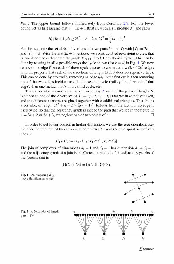
For this, separate the set of 3k+1 vertices into two parts V1 and V2 with |V1| = 2k+1and |V2| = k. With the first 2k + 1 vertices, we construct k edge-disjoint cycles, thatis, we decompose the complete graph K2k+1 into k Hamiltonian cycles. This can bedone by rotating in all k possible ways the cycle shown (for k = 4) in Fig. 1. We nowremove one edge from each of these cycles, so as to construct a walk of 2k2 edgeswith the property that each of the k sections of length 2k in it does not repeat vertices.This can be done by arbitrarily removing an edge i0i1 in the first cycle, then removingone of the two edges incident to i1 in the second cycle (call i2 the other end of thatedge), then one incident to i2 in the third cycle, etc.
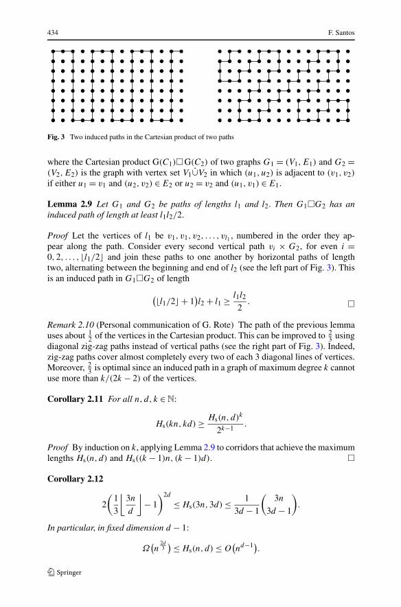
Then a corridor is constructed as shown in Fig. 2: each of the paths of length 2k
is joined to one of the k vertices of V2 = {j1, j2, . . . , jk} that we have not yet used,and the different sections are glued together with k additional triangles. That this isa corridor, of length 2k2 + k − 2 ≥ 2
9 (n − 1)2, follows from the fact that no edge isused twice, so that the adjacency graph is indeed the path that we see in the figure. Ifn = 3k + 2 or 3k + 3, we neglect one or two points of n. �
In order to get lower bounds in higher dimension, we use the join operation. Re-member that the join of two simplicial complexes C1 and C2 on disjoint sets of ver-tices is
C1 ∗ C2 := {v1 ∪ v2 : v1 ∈ C1, v2 ∈ C2}.The join of complexes of dimensions d1 − 1 and d2 − 1 has dimension d1 + d2 − 1and the adjacency graph of a join is the Cartesian product of the adjacency graphs ofthe factors; that is,
G(C1 ∗ C2) = G(C1)�G(C2),
Fig. 1 Decomposing K2k+1into k Hamiltonian cycles
Fig. 2 A 2-corridor of length29 (n − 1)2
434 F. Santos
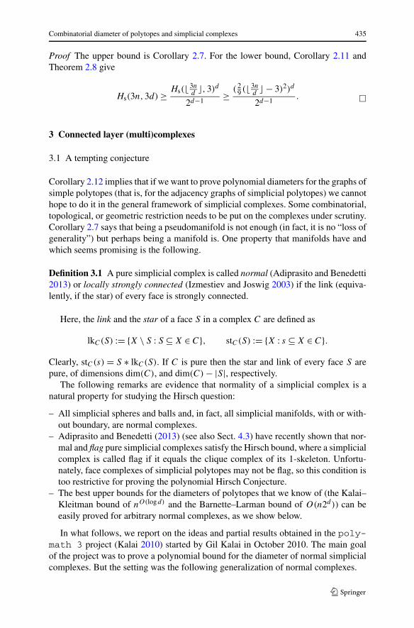
Fig. 3 Two induced paths in the Cartesian product of two paths
where the Cartesian product G(C1)�G(C2) of two graphs G1 = (V1,E1) and G2 =(V2,E2) is the graph with vertex set V1∪̇V2 in which (u1, u2) is adjacent to (v1, v2)
if either u1 = v1 and (u2, v2) ∈ E2 or u2 = v2 and (u1, v1) ∈ E1.
Lemma 2.9 Let G1 and G2 be paths of lengths l1 and l2. Then G1�G2 has aninduced path of length at least l1l2/2.
Proof Let the vertices of l1 be v1, v1, v2, . . . , vl1 , numbered in the order they ap-pear along the path. Consider every second vertical path vi × G2, for even i =0,2, . . . , �l1/2� and join these paths to one another by horizontal paths of lengthtwo, alternating between the beginning and end of l2 (see the left part of Fig. 3). Thisis an induced path in G1�G2 of length
(�l1/2� + 1)l2 + l1 ≥ l1l2
2. �
Remark 2.10 (Personal communication of G. Rote) The path of the previous lemmauses about 1
2 of the vertices in the Cartesian product. This can be improved to 23 using
diagonal zig-zag paths instead of vertical paths (see the right part of Fig. 3). Indeed,zig-zag paths cover almost completely every two of each 3 diagonal lines of vertices.Moreover, 2
3 is optimal since an induced path in a graph of maximum degree k cannotuse more than k/(2k − 2) of the vertices.
Corollary 2.11 For all n,d, k ∈N:
Hs(kn, kd) ≥ Hs(n, d)k
2k−1.
Proof By induction on k, applying Lemma 2.9 to corridors that achieve the maximumlengths Hs(n, d) and Hs((k − 1)n, (k − 1)d). �
Corollary 2.12
2
(1
3
⌊3n
d
⌋− 1
)2d
≤ Hs(3n,3d) ≤ 1
3d − 1
(3n
3d − 1
).
In particular, in fixed dimension d − 1:
Ω(n
2d3) ≤ Hs(n, d) ≤ O
(nd−1).
Combinatorial diameter of polytopes and simplicial complexes 435
Proof The upper bound is Corollary 2.7. For the lower bound, Corollary 2.11 andTheorem 2.8 give
Hs(3n,3d) ≥ Hs(� 3nd
�,3)d
2d−1≥ ( 2
9 (� 3nd
� − 3)2)d
2d−1. �
3 Connected layer (multi)complexes
3.1 A tempting conjecture
Corollary 2.12 implies that if we want to prove polynomial diameters for the graphs ofsimple polytopes (that is, for the adjacency graphs of simplicial polytopes) we cannothope to do it in the general framework of simplicial complexes. Some combinatorial,topological, or geometric restriction needs to be put on the complexes under scrutiny.Corollary 2.7 says that being a pseudomanifold is not enough (in fact, it is no “loss ofgenerality”) but perhaps being a manifold is. One property that manifolds have andwhich seems promising is the following.
Definition 3.1 A pure simplicial complex is called normal (Adiprasito and Benedetti2013) or locally strongly connected (Izmestiev and Joswig 2003) if the link (equiva-lently, if the star) of every face is strongly connected.
Here, the link and the star of a face S in a complex C are defined as
lkC(S) := {X \ S : S ⊆ X ∈ C}, stC(S) := {X : s ⊆ X ∈ C}.Clearly, stC(s) = S ∗ lkC(S). If C is pure then the star and link of every face S arepure, of dimensions dim(C), and dim(C) − |S|, respectively.
The following remarks are evidence that normality of a simplicial complex is anatural property for studying the Hirsch question:
– All simplicial spheres and balls and, in fact, all simplicial manifolds, with or with-out boundary, are normal complexes.
– Adiprasito and Benedetti (2013) (see also Sect. 4.3) have recently shown that nor-mal and flag pure simplicial complexes satisfy the Hirsch bound, where a simplicialcomplex is called flag if it equals the clique complex of its 1-skeleton. Unfortu-nately, face complexes of simplicial polytopes may not be flag, so this condition istoo restrictive for proving the polynomial Hirsch Conjecture.
– The best upper bounds for the diameters of polytopes that we know of (the Kalai–Kleitman bound of nO(logd) and the Barnette–Larman bound of O(n2d)) can beeasily proved for arbitrary normal complexes, as we show below.
In what follows, we report on the ideas and partial results obtained in the poly-math 3 project (Kalai 2010) started by Gil Kalai in October 2010. The main goalof the project was to prove a polynomial bound for the diameter of normal simplicialcomplexes. But the setting was the following generalization of normal complexes.
436 F. Santos
Definition 3.2 A pure multicomplex of rank d on n elements is a collection M ofmultisets of size d of [n] (or of any other set V of size n). Here, a multiset is anunordered set of elements of [n] with repetitions allowed. Formally, a multiset of sized can be modeled as a degree d monomial in K[x1, . . . , xn].
We keep for multicomplexes the notions defined for complexes, such as facet,face, link, etc. For example, the star and the link of a face S in M are
lkM(S) := {X \ S : S ⊆ X ∈ C}, stM(S) := {X : s ⊆ X ∈ C}.But, of course, set operations have to be understood in the multiset sense. The inter-section of two multisets A and B is the multiset that contains each element of [n] withthe minimum number of repetitions it has in A or B , and the union is the same withminimum replaced to maximum. If multisets are modeled as monomials, intersectionand union become gcd and lcm. We also keep for multicomplexes the definitions ofdual graph, diameter, and of being strongly connected or normal.
We now get to the main definition in this section.
Definition 3.3 A connected layer multicomplex (or c.l.m., for short), is a pure multi-complex M together with a partition M = La∪̇La+1∪̇ · · · ∪̇Lb (with a, b ∈ Z, a ≤ b)of its set of facets into layers having the following connectedness property:
For every mutisubset S, the star of S intersects an interval of layers. (1)
The length of a c.l.m. is b − a, that is, one less than the number of layers.
In particular, we are interested in the function:
Hc.l.m.(n, d) := maximum length of c.l.m.’s of rank d with [n] elements.
This definition, and some of the results below, were first introduced by Eisen-brand et al. (2010) except they considered usual complexes instead of multicomplexes.The generalization to multicomplexes was proposed by Hähnle in the polymath 3project (Kalai 2010), where he also made the following conjecture:
Conjecture 3.4 (Hähnle-polymath 3 (Kalai 2010))
∀n,d, Hc.l.m.(n, d) ≤ d(n − 1).
Remark 3.5 This conjecture would imply, by Proposition 3.7 below, the same boundfor the diameter of every normal simplicial multicomplex of dimension d − 1 on n
vertices. In particular, for the graph-diameter of d-polytopes with n facets.
Let us be more explicit about condition (1). What we mean is that for every mul-tiset S, if there are facets that contain S in layers Li and Lj , then there is also a facetcontaining S in every intermediate layer. This easily implies the following proposi-tion.
Combinatorial diameter of polytopes and simplicial complexes 437
Proposition 3.6 Let M be a c.l.m. of rank d on n elements. Then for every face S,the link of S in M is a c.l.m. of rank d − |S| on (at most) n elements, where the ithlayer of lkM(S) is defined to be lkLi
(S).
Every normal multicomplex M can naturally be turned into a c.l.m. of lengthequal to the diameter of M . For this, let X and Y be facets of M at distance equalto the diameter of M . We layer M by “distance to X”. That is, we let Li contain allthe facets that are at distance i to X in the adjacency graph of M (e.g., L0 = {X}).Normality of M implies the connectedness condition (1). Hence:
Proposition 3.7 The maximum diameter among all normal multicomplexes of rankd with n elements is smaller or equal than Hc.l.m.(n, d).
3.2 Two extremal cases
We call a c.l.m. complete if its underlying multicomplex is complete; that is, each ofthe
(n+d−1
d
)multisubsets of [n] of size d is used in some layer. We call it injective if
each layer has a single facet, that is, the map M → Z that assigns facets to its layers isinjective. These two classes of c.l.m.’s are extremal and opposite, in the sense that thecomplete c.l.m.’s have the maximum number of facets for given n and d and injectiveones the minimum possible number for a given length.
Example 3.8 (A complete c.l.m., polymath 3 (Kalai 2010)) For any d and n, considerthe complete multicomplex of rank d on the set [n]. Consider it layered putting inlayer i (i = d, . . . , nd) all the facets with sum of elements equal to i. This is a c.l.m.
of length d(n − 1).
Example 3.9 (An injective c.l.m., polymath 3 (Kalai 2010)) For any d and n, considerthe multicomplex of rank d on [n] consisting of all the multisets using at most twodifferent elements from [n], and consecutive ones. For example, for n = 4, d = 3 ourmulticomplex is
{111,112,122,222,233,233,333,334,344,444}.Consider it layered with the restriction of the layering in the previous example. Thisproduces an injective c.l.m. of the same length d(n − 1).
Proposition 3.10 (Polymath 3 (Kalai 2010)) Let M = La∪̇ · · · ∪̇Lb be a connectedlayer multicomplex of rank d on n elements. If M is either complete or injective, thenits length is at most d(n − 1).
Proof If M is complete, we proceed by induction on d , the case d = 1 being trivial.Let X ∈ La and Y ∈ Lb be facets in the first and last layer, respectively, and let i andj be elements in X \Y and Y \X, respectively (these formulas have to be understoodin the multiset sense. That is, i ∈ X \ Y means that i appears more times in X thanin Y ). Let X′ = X \ {i} ∪ {j}, which must be in some layer Lc. Since X and X′ differon a single element, c − a ≤ n − 1 (the link of X ∩ X′ in M is a c.l.m. of rank d).
438 F. Santos
On the other hand, the link of j in M is a c.l.m. of rank d − 1 on n elements andit intersects (at least) the layers from c to b of M , so that b − c ≤ (n − 1)(d − 1).Putting this together:
b − a = (b − c) + (c − a) ≤ (n − 1)(d − 1) + (n − 1) = d(n − 1).
For the injective case, we observe that the degree of each element i ∈ [n] in thesequence of layers of M is a unimodal function: it (weakly) increases up to a certainpoint and then it decreases. In particular, there are at most d steps where the degree ofi increases from one layer to the next. On the other hand, at least one degree increasesat each step, so the number of steps is at most dn. This bound decreases to dn − d ifwe observe that in the first layer some degrees where already positive; more precisely,the initial sum of degrees is exactly d . �
Proposition 3.10 is quite remarkable. It shows that in two “extremal and opposite”cases of connected layer multicomplexes we have an upper bound of d(n − 1) fortheir length. And Examples 3.8 and 3.9 show that this bound is attained in both cases.This is, in our opinion, what makes Conjecture 3.4 exciting.
3.3 Two upper bounds
Here, we show that the two best upper bounds on diameters of polytopes that weknow of can actually be proved in the context of c.l.m.’s.
Lemma 3.11 For every n and d we have
Hc.l.m.(n, d) ≤ Hc.l.m.
(⌊n − 1
2
⌋, d
)+Hc.l.m.
(⌈n − 1
2
⌉, d
)+Hc.l.m.(n, d −1)+2.
Proof Let M be a c.l.m. of rank d on n elements. Let i be the largest integer such thatthe first i layers of M use at most �(n − 1)/2� of the n elements. Let j be the largestinteger such that the last j layers of M use at most �(n− 1)/2� of the n elements. Letk be the remaining number of layers. By construction, there has to be some commonelement used in all these k layers. Hence,
i − 1 ≤ Hc.l.m.
(�n/2�, d),
j − 1 ≤ Hc.l.m.
(�n/2�, d),
k − 1 ≤ Hc.l.m.(n, d − 1).
This gives the bound, since the length of our c.l.m. equals i + j + k − 1. �
Theorem 3.12 (Kalai and Kleitman 1992; Eisenbrand et al. 2010)
Hc.l.m.(n, d) ≤ nlog2 d+1 − 1
Combinatorial diameter of polytopes and simplicial complexes 439
Proof We assume that both n and d are at least equal to 2, or else the statement istrivial (and the inequality is tight). For later use, we observe that, under these con-straints:
n ≤ 2n2
4= 2 · 4log2 n−1 ≤ 2(2d)log2 n−1. (2)
Let us now convert the inequality of Lemma 3.11 in something more usable. Let-ting f (n, d) := Hc.l.m.(n, d) + 1 and taking into account that �n−1
2 � ≤ �n−12 � ≤ �n
2 �(plus monotonicity of Hc.l.m.) we get
f (n, d) ≤ 2f(�n/2�, d) + f (n, d − 1).
Applying this recursively, we get
f (n, d) ≤ 2d∑
i=2
f(�n/2�, i) + f (n,1) ≤ 2(d − 1)f
(�n/2�, d) + n. (3)
Now, by inductive hypothesis,
f(�n/2�, d) ≤
(n
2
)log2 d+1
= (2d)log2 n−1.
Plugging this into (3), and using (2) gives
f (n, d) ≤ 2(d − 1)(2d)log2 n−1 + n ≤ (2d)log2 n = nlog2 2d . �
Lemma 3.13 For every c.l.m. M of rank d on n elements there are n1, . . . , nk with∑ni ≤ 2n − 1 and such that the length of M is bounded above by
Hc.l.m.(n1, d − 1) + · · · + Hc.l.m.(nk, d − 1) + k − 1.
Proof Let L0, . . . ,LN be the layers of M . Let l1 be the last layer such that L0 andLl1 use some common vertex, and let n1 be the number of vertices used in the layersL0 ∪· · ·∪Ll1 . Clearly, l1 ≤ Hc.l.m.(n1, d −1). Apply the same to the remaining layersLl1+1, . . . ,LN . That is to say, let l2 be the last layer that shares a vertex with Ll1+1and let n2 be the vertices used in Ll1+1, . . . ,Ll2 , etc.
At the end, we have decomposed M into several (say k) connected layer multi-complexes so, indeed, its length is the sum of the k lengths plus k − 1. Since the ithsub-multicomplex has the property that it uses ni elements and one of them is usedin all layers, its length is at most Hc.l.m.(ni, d − 1).
It only remains to be shown that∑
ni ≤ 2n − 1. That∑
ni ≤ 2n comes fromthe fact that no vertex can be used in more that two of the sub-multicomplexes, byconstruction of them. The −1 from the fact that vertices used in L0 cannot be used inany sub-multicomplex other than the first one. �
Theorem 3.14 (Larman 1970; Barnette 1974; Eisenbrand et al. 2010)
Hc.l.m.(n, d) ≤ (n − 1)2d−1.
440 F. Santos
Proof By induction on d , with the case d = 1 being trivial. For the general case, letM be a c.l.m. of maximal length equal to Hc.l.m.(n, d) and use the decomposition ofLemma 3.13. This gives
Hc.l.m.(n, d) ≤k∑
i=1
Hc.l.m.(ni, d − 1) + k − 1
≤k∑
i=1
(ni − 1)2d−2 + k − 1
≤ (2n − k − 1)2d−2 + k − 1
= (n − 1)2d−1 − (k − 1)(2d−2 − 1
) ≤ (n − 1)2d−1. �
Corollary 3.15 If n ≤ 3 or d ≤ 2, then
Hc.l.m.(n, d) = (n − 1)d.
Proof By Examples 3.8 and 3.9, we only need to prove the upper bound. In the casesn ≤ 2 or d = 1, we have that (n − 1)d + 1 = (
n+d−1d
), which is the number of facets
in the complete multicomplex, so the bound is trivial. The case d = 2 follows fromTheorem 3.14 and the case n = 3 from Lemma 3.11. �
Besides the values in this corollary, Kalai (2010) has verified Conjecture 3.4 forall values of (n, d) in or below {(4,13), (5,7), (6,5), (7,4), (8,3)}.
3.4 Variations on the theme of c.l.m.’s
What is contained above are the main properties and results on connected layer mul-ticomplexes and, in particular, the main outcome of the polymath 3 project. But itmay be worth mentioning other related ideas, questions, and loose ends.
3.4.1 Complexes versus multicomplexes
Connected layer multicomplex were introduced in Kalai (2010) based on previouswork of Eisenbrand et al. (2010) in which they introduced connected layer com-plexes (under the name connected layer families). The definition is exactly the sameas Definition 3.3 except M is now a pure simplicial complex, rather than a multi-complex. Since the concept is more restricted, all the upper bounds that we provedfor c.l.m.’s (Proposition 3.10, Theorems 3.12, and 3.14) are still valid for connectedlayer complexes. The question is whether multicomplexes allow for longer objectsthan complexes. The following result says that “not much more.” In it, Hc.l.c.(n, d)
denotes the maximum length of connected layer complexes of rank d on n elements.
Theorem 3.16 (Polymath 3 (Kalai 2010))
Hc.l.c.(n, d) ≤ Hc.l.m.(n, d) ≤ Hc.l.c.(nd, d).
Combinatorial diameter of polytopes and simplicial complexes 441
Proof The first inequality is obvious. For the second one, let M be a c.l.m. of rank d
on n elements achieving Hc.l.m.(n, d). We can construct a connected layer complexof the same length and rank on the set [n] × [d] simply by the following substitutionof multisets to sets:
{1k1, . . . , nkn
} �→ {(1,1), . . . , (1, k1), . . . , (n,1), . . . , (n, kn)
}. �
As further evidence, one of the main results of Eisenbrand et al. (2010) is theconstruction of connected layer complexes showing that
Hc.l.c.(4d, d) ≥ Ω(d2/ logd
),
which is not far from the upper bound (4d − 1)d in Conjecture 3.4.Similarly, in the polymath 3 project it was shown that
2n − O(√
n) ≤ Hc.l.c.(n,2) ≤ Hc.l.m.(n,2) = 2n − 2.
These inequalities are interesting for two reasons. On the one hand, they point againinto the direction of Hc.l.m.(n, d) and Hc.l.c.(n, d) not being too different. But theyalso highlight the fact that Hc.l.m.(n, d) is more tractable than Hc.l.c.(n, d). We knowthe exact value of Hc.l.m.(n,2) but not that of Hc.l.c.(n,2), despite quite some effortdevoted in the polymath 3 project to this very specific question.
3.4.2 Specific values for small n or d
Not much is known on this besides Corollary 3.15. In particular, for Hc.l.m.(n,3) weonly know
3n − 3 ≤ Hc.l.m.(n,3) ≤ 4n − 4.
The lower bound comes from Examples 3.9 and 3.8, while the upper bound comesfrom Theorem 3.14. Some effort was devoted (with no success) to deciding whichof the two bounds is closer to the truth, since the answer would be an indicationof whether Hc.l.m.(n,3) behaves polynomially or not. Of course, the lower bound issimply the value predicted by Conjecture 3.4.
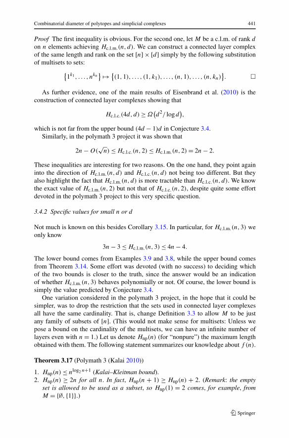
One variation considered in the polymath 3 project, in the hope that it could besimpler, was to drop the restriction that the sets used in connected layer complexesall have the same cardinality. That is, change Definition 3.3 to allow M to be justany family of subsets of [n]. (This would not make sense for multisets: Unless wepose a bound on the cardinality of the multisets, we can have an infinite number oflayers even with n = 1.) Let us denote Hnp(n) (for “nonpure”) the maximum lengthobtained with them. The following statement summarizes our knowledge about f (n).
Theorem 3.17 (Polymath 3 (Kalai 2010))
1. Hnp(n) ≤ nlog2 n+1 (Kalai–Kleitman bound).2. Hnp(n) ≥ 2n for all n. In fact, Hnp(n + 1) ≥ Hnp(n) + 2. (Remark: the empty
set is allowed to be used as a subset, so Hnp(1) = 2 comes, for example, fromM = {∅, {1}}.)
442 F. Santos
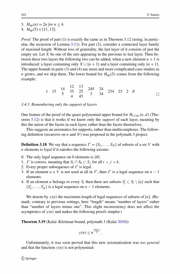
3. Hnp(n) = 2n for n ≤ 4.4. Hnp(5) ∈ [11,12].
Proof The proof of part (1) is exactly the same as in Theorem 3.12 (using, in partic-ular, the recursion of Lemma 3.11). For part (2), consider a connected layer familyof maximal length. Without loss of generality, the last layer of it consists of just theempty set. Let X be one of the sets appearing in the previous to last layer. Then be-tween these two layers the following two can be added, when a new element n + 1 isintroduced: a layer containing only X ∪ {n + 1} and a layer containing only {n + 1}.The upper bounds in parts (3) and (4) use more and more complicated case-studies asn grows, and we skip them. The lower bound for Hnp(5) comes from the followingexample:
1 15145
12354
132545
2453
2434
234 23 2 ∅ �
3.4.3 Remembering only the support of layers
One feature of the proof of the quasi-polynomial upper bound for Hc.l.m.(n, d) (The-orem 3.12) is that it works if we know only the support of each layer, meaning bythis the union of the facets in each layer, rather than the facets themselves.
This suggests an axiomatics for supports, rather than multicomplexes. The follow-ing definition (recursive on n and N ) was proposed in the polymath 3 project.
Definition 3.18 We say that a sequence Γ = {S1, . . . , SN } of subsets of a set V withn elements is legal if it satisfies the following axioms:
0. The only legal sequence on 0 elements is {∅}.1. Γ is convex, meaning that Si ∩ Sk ⊂ Sj for all i < j < k.2. Every proper subsequence of Γ is legal.3. If an element a ∈ V is not used at all in Γ , then Γ is a legal sequence on n − 1
elements.4. If an element a belongs to every Si then there are subsets S′
i ⊂ Si \ {a} such that{S′
1, . . . , S′N } is a legal sequence on n − 1 elements.
We denote by y(n) the maximum length of legal sequences of subsets of [n]. (Re-mark: contrary to previous settings, here “length” means “number of layers” ratherthan “number of layers minus one”. This slight inconsistency does not affect theasymptotics of y(n) and makes the following proofs simpler.)
Theorem 3.19 (Kalai–Kleitman bound, polymath 3 (Kalai 2010))
y(n) ≤ nlog2 n
2 .
Unfortunately, it was soon proved that this new axiomatization was too generaland that the function y(n) is not polynomial:
Combinatorial diameter of polytopes and simplicial complexes 443
Lemma 3.20 For every n and i,
y(2(n + i)
) ≥ (i + 1)y(n).
Proof For i = 1, observe that the sequence with y(n) copies of a set A of size n + 1is valid on n + 1 elements. Taking two disjoint sets A and B of the same size, thesequence
(A, . . . ,A,B, . . . ,B),
where each block has length y(n), shows y(2n + 2) ≥ 2y(n).The same idea shows (by induction on i) the general statement: sets if A and B
are disjoint with n + i elements, then the sequence
(A, . . . ,A,A ∪ B, . . . ,A ∪ B,B, . . . ,B),
where the blocks of A’s and B’s have length y(n) and the block of A∪B’s has length(i − 1)y(n) is legal. �
Corollary 3.21 (Polymath 3 (Kalai 2010))
1. y(4n) ≥ ny(n) for all n.
2. y(4k) ≥ 4(k2).
Proof For part (1), let i = n in the lemma. For part (2), use part (1) and inductionon k. �
Observe that this is not far from the upper bound of Theorem 3.19, which special-izes to
y(4n
) ≤ 4k2.
3.4.4 Reformulations and other abstractions
The connected layer complexes and multicomplexes that we have been consideringin this section are certainly not the first attempt at proving the Hirsch Conjecture (ora polynomial version of it) by generalizing and abstracting the properties of graphsof polytopes. Other classical attempts are for example in Adler and Dantzig (1974)and Kalai (1992). (The second one can be considered a prequel to the Kalai–Kleitmanquasi-polynomial upper bound.) In fact, these earlier attempts were an inspiration forthe work of Eisenbrand et al. (2010).
Taking this into account, Kim (2013) started a study of variations of the axiomsdefining connected layer complexes. His main generalization is that instead of thelayers forming a sequence, he allows for them to be attached to the vertices of anarbitrary graph G, whose diameter we want to bound. The connectedness conditionposed for c.l.m.’s or c.l.c.’s (condition (1) of Definition 3.3) becomes:
∀S ⊂ [n], the star of S intersects a connected subgraph of layers. (4)
Apart of this, Kim considers also the following properties, that can be posed forthese objects:
444 F. Santos
– Adjacency: if two facets of M differ by a single element then they must lie in thesame or adjacent layers. (That is, the map from G(M) to G associating each facetto its layer is simplicial.)
– Strong adjacency: adjacency holds and every two adjacent layers contain facetsdiffering by an element.
– Pseudomanifold, or end-point count: no codimension one face of M is containedin more than two facets of M .
Among his results are a generalization of the Kalai–Kleitman bound for all layercomplexes satisfying connectivity, and some examples showing that without connec-tivity exponential diameters (of the graph G) can occur. For example, diameter nd/4
can be obtained for layer complexes that have the end-point count and the strong-adjacency properties. Similar examples were later obtained by Hähnle (2012).
4 Recent results on the diameter of polytopes and polyhedra
4.1 Exact bounds for small d and n
Remember that we denote by Hp(n,d) the maximum diameter among all d-polyhedra with n facets. The version restricted to bounded polytopes will be de-noted Hb(n, d). It is easy to show that Hp(n,d) ≥ Hb(n, d) for all n > d and thatHp(n,d) ≥ n − d for all n and d . The latter is not true for Hb(n, d) (e.g., it is clearthat Hb(n,2) = �n/2�).
In this section, we report on what exact values of Hb(n, d) are known. The recentpart are the papers (Bremner et al. 2013; Bremner and Schewe 2011), but let us startwith a bit of history. The Hirsch Conjecture was soon proved to hold for polytopesand polyhedra of dimension 3 (we here state only the version for polytopes). A proofcan be found in Kim and Santos (2010).
Theorem 4.1 (Klee 1966) Hb(n,3) = � 2n3 � − 1.
In fact, the lower bound in this statement is easy to generalize. Observe that theformula below gives the exact value of Hb(n, d) for d = 2 as well. Proofs of Theo-rem 4.1 and Proposition 4.2 can be found in Kim and Santos (2009).
Proposition 4.2
Hb(n, d) ≥⌊
d − 1
dn
⌋− (d − 2).
On the other extreme, when n − d , rather than d , is small, there is also the fol-lowing classical and important statement of Klee and Walkup. A proof can be foundin Kim and Santos (2010, Theorem 3.2).
Theorem 4.3 (Klee and Walkup 1967) Fix a positive integer k. Then maxd H(d +k, d) = H(2d, d).
Combinatorial diameter of polytopes and simplicial complexes 445
Here, we write H(n,d) without a subscript because the statement is valid forbounded polytopes, for unbounded polyhedra, and for much more general objects(e.g., normal (d − 1)-spheres or balls). In the same paper, Klee and Walkup showedthat Hb(10,5) = 5. With this, they concluded the Hirsch Conjecture for polytopeswith n − d ≤ 5. Goodey (1972) computed Hb(10,4) = 5 and Hb(11,5) = 6, but wasnot able to certify that Hb(12,6) = 6. This was done only recently by Bremner andSchewe (2011).
Corollary 4.4 (Bremner and Schewe 2011) The Hirsch bound holds for polytopeswith at most six facets more than their dimension.
The work from Bremner and Schewe (2011) was later extended by the same au-thors together with Deza and Hua, which computed Hb(12,4) = Hb(12,5) = 7. Allin all, the following statement exhausts all pairs (n, d) for which the maximum di-ameter Hb(n, d) of d-polytopes with n facets is known. We omit the cases n < 2d ,because Hb(d + k, d) = Hb(2k, k) for all k < d (see Theorem 4.3), and the trivialcase d ≤ 2.
Theorem 4.5
– Hb(8,4) = 4 (Klee 1966).– Hb(9,4) = Hb(10,5) = 5 (Klee and Walkup 1967).– Hb(10,4) = 5, Hb(11,5) = 6 (Goodey 1972).– Hb(11,4) = Hb(12,6) = 6 (Bremner and Schewe 2011).– Hb(12,4) = Hb(12,5) = 7 (Bremner et al. 2013).
The results in Bremner et al., Bremner and Schewe (2013, 2011) involve heavyuse of computer power. But it would be unfair to say that they are obtained by “bruteforce.” In fact, brute force enumeration of the combinatorial types of polytopes with12 facets is beyond today’s possibilities.
Instead of that the authors look, for each pair (n, d) under study, at the possiblepath complexes, where a path complex is a simplicial complex of dimension d − 1with n vertices and with certain axiomatic restrictions that are necessary for it to be asubcomplex of a simplicial polytope. After enumerating path complexes, the authorsaddress the question of which of them can be completed to be part of the boundaryof an actual polytope without the completion producing “shortcuts.” This is modeledin oriented matroid terms: For the path complex to be part of a polytope boundary,certain signs are needed in the chirotope of the polytope. The question of whether ornot a chirotope with those sign constraints exists is solved with a standard SAT solver,using some ad-hoc decompositions in the instances that are too large for the solverto decide. The reduction to satisfiability follows ideas of Schewe (2009) developedoriginally for a different realizability question.
4.2 Polytope counterexamples to the Hirsch Conjecture
The Hirsch Conjecture for unbounded polyhedra was disproved in 1967 by Klee andWalkup, who showed the following.
446 F. Santos
Theorem 4.6 (Klee and Walkup 1967) There is a 4-polyhedron with 5 facets anddiameter five.
See Kim and Santos (2009, 2010) for a relatively simple description of the Klee–Walkup polyhedron, and its relation to a Hirsch-sharp 4-polytope with nine facets andto the disproof by Todd (1980) of the “monotone Hirsch Conjecture.” The parametersn and d in this example are smallest possible, as Klee and Walkup also showed. More-over, it was later shown by Altshuler et al. (1980) that the Klee–Walkup non-Hirschpolyhedron is unique among simple polyhedra with that dimension and number offacets: Every 4-polyhedron with 8 facets not combinatorially equivalent to it satisfiesthe Hirsch bound.
But the same paper of Klee and Walkup contains the more relevant (in our opinion)result that we stated as Theorem 4.3: that the Hirsch Conjecture (be it for polytopes,polyhedra, or simplicial balls and spheres) is equivalent to the special case n = 2d .This special case was dubbed the d-step conjecture since it states that we can go fromany vertex to any other vertex in (at most) d-steps. This result of Klee and Walkupwas based in the following easy lemma (see, e.g., Kim and Santos 2010, Lemma 3.1):
Lemma 4.7 (d-Step Lemma, Klee and Walkup 1967) Let P be a polyhedron with n
facets, dimension d , and a certain diameter δ. Then, by a wedge on any facet of P ,we obtain another polyhedron P ′ of dimension d + 1, with n + 1 facets and withdiameter (at least) δ.
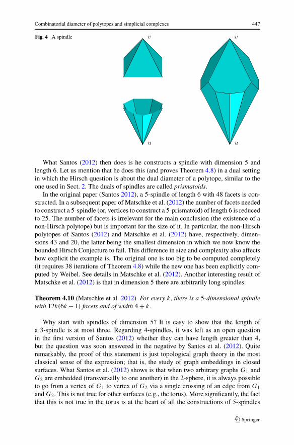
The first ingredient in the construction of bounded counter-examples to the HirschConjecture is a stronger version of the d-step lemma for a particular class of poly-topes. We call a polytope a spindle if it has two specified vertices u and v such thatevery facet contains exactly one of them. Put differently, a spindle is the intersectionof two pointed cones with apices at u and v (see Fig. 4). The length of a spindle isthe graph distance between u and v. Spindles that are simple at u and v coincide withwhat are classically called Dantzig figures. Our statement is, however, about spindlesthat are not simple:
Theorem 4.8 (Strong d-step lemma, Santos 2012) Let P be a spindle with n facets,dimension d , and a certain length l, and suppose n > 2d . Then, by a wedge on acertain facet of P followed by a perturbation, we can obtain another spindle P ′ ofdimension d + 1, with n + 1 facets and with length (at least) l + 1.
Observe that this statement is stronger than the classical d-step lemma only in the“+1” in l. This is enough, however, to obtain the following crucial corollary.
Corollary 4.9 If a spindle P has length greater than its dimension, then applyingTheorem 4.8 n − 2d times we obtain a polyhedron violating the Hirsch Conjecture.More precisely, from a d-spindle with n > 2d facets and length l > d we obtain apolyhedron of dimension D = n− d , with N = 2(n− d) facets, and diameter at leastl + (n − 2d) > D = N − D.
Combinatorial diameter of polytopes and simplicial complexes 447
Fig. 4 A spindle
What Santos (2012) then does is he constructs a spindle with dimension 5 andlength 6. Let us mention that he does this (and proves Theorem 4.8) in a dual settingin which the Hirsch question is about the dual diameter of a polytope, similar to theone used in Sect. 2. The duals of spindles are called prismatoids.
In the original paper (Santos 2012), a 5-spindle of length 6 with 48 facets is con-structed. In a subsequent paper of Matschke et al. (2012) the number of facets neededto construct a 5-spindle (or, vertices to construct a 5-prismatoid) of length 6 is reducedto 25. The number of facets is irrelevant for the main conclusion (the existence of anon-Hirsch polytope) but is important for the size of it. In particular, the non-Hirschpolytopes of Santos (2012) and Matschke et al. (2012) have, respectively, dimen-sions 43 and 20, the latter being the smallest dimension in which we now know thebounded Hirsch Conjecture to fail. This difference in size and complexity also affectshow explicit the example is. The original one is too big to be computed completely(it requires 38 iterations of Theorem 4.8) while the new one has been explicitly com-puted by Weibel. See details in Matschke et al. (2012). Another interesting result ofMatschke et al. (2012) is that in dimension 5 there are arbitrarily long spindles.
Theorem 4.10 (Matschke et al. 2012) For every k, there is a 5-dimensional spindlewith 12k(6k − 1) facets and of width 4 + k.
Why start with spindles of dimension 5? It is easy to show that the length ofa 3-spindle is at most three. Regarding 4-spindles, it was left as an open questionin the first version of Santos (2012) whether they can have length greater than 4,but the question was soon answered in the negative by Santos et al. (2012). Quiteremarkably, the proof of this statement is just topological graph theory in the mostclassical sense of the expression; that is, the study of graph embeddings in closedsurfaces. What Santos et al. (2012) shows is that when two arbitrary graphs G1 andG2 are embedded (transversally to one another) in the 2-sphere, it is always possibleto go from a vertex of G1 to vertex of G2 via a single crossing of an edge from G1and G2. This is not true for other surfaces (e.g., the torus). More significantly, the factthat this is not true in the torus is at the heart of all the constructions of 5-spindles
448 F. Santos
of length greater than 5, via the standard Clifford embedding of the torus in the 3-sphere and a reduction of the combinatorics of 5-spindles to the study of certain celldecompositions of the 3-sphere.
In the rest of this section, we study how good (or how bad) the counter-examplesto the Hirsch Conjecture that can be obtained with this spindle method are. Follow-ing Santos (2012), we call (Hirsch) excess of a d-polytope P with n facets and diam-eter δ the quantity
δ
n − d− 1.
This is positive if and only if the diameter of P exceeds the Hirsch bound. Excess is asignificant parameter since, as shown in Santos (2012, Sect. 6), from any non-Hirschpolytope one can obtain infinite families of them with (essentially) the same excessas the original, even in fixed (but high) dimension.
Theorem 4.11 (Santos 2012) Let P be a non-Hirsch polytope of dimension d andexcess ε. Then for each k ∈ N there is an infinite family of non-Hirsch polytopes ofdimension kd and with excess greater than
(1 − 1
k
)ε.
The excess of the non-Hirsch polytope produced via Theorem 4.8 from a d-spindleP of length l and n vertices equals
l − d
n − d,
so we call this quotient the (spindle) excess of P . The spindle of Matschke et al.(2012), hence also the non-Hirsch polytope obtained from it, has excess 1/20. Thisis the greatest excess of a spindle or polytope constructed so far. (The excess of theKlee–Walkup unbounded non-Hirsch polyhedron is, however, 1/4.)
It could seem that the arbitrarily long spindles mentioned in Theorem 4.10 shouldlead to non-Hirsch polytopes of greater excess. This is not the case, however, becausetheir number of facets grows quadratically with the length. So, asymptotically, theirspindle excess is zero.
On the side of upper bounds, the Barnette–Larman general bound for the diame-ters of polytopes (Larman 1970) (see the version for connected layer families in The-orem 3.14) implies that the excess of spindles of dimension d cannot exceed 2d−2/3.For dimension 5, this is improved to 1/3 in Matschke et al. (2012). What are the im-plications of this? Of course, using spindles of higher dimension it may be possibleto get non-Hirsch polytopes of great excess. But the main point of the spindle methodis that it relates non-Hirschness to length and dimension alone, regardless of numberof facets or vertices, which gives a lot of freedom to construct complicated spindlesin fixed dimension. It seems to us that giving up “fixed dimension” in this methodleads to a problem as complicated as the original Hirsch question. On the other hand,Barnette–Larman’s bound implies that the method in fixed dimension cannot produce
Combinatorial diameter of polytopes and simplicial complexes 449
non-Hirsch polytopes whose excess is more than a constant. That is, the method doesnot seem to be good enough to disprove a “linear Hirsch Conjecture” (in case it isfalse).
4.3 The Hirsch Conjecture holds for flag normal complexes
A simplicial complex C is a flag complex (or a clique complex) if, whenever the graphof C contains the complete graph on a certain subset S of vertices, we have that S isa face in C. (Here, we mean the usual graph of C, not the adjacency or dual graph).Equivalently, C is flag if every minimal nonface (that is, every inclusion minimalsubset of vertices that is not a face) has cardinality two. Examples of flag complexesinclude the barycentric subdivisions of arbitrary simplicial complexes.
In this section, we reproduce Adiprasito and Benedetti’s recent proof of the Hirschbound for simple polytopes whose polar simplicial complex is flag (Adiprasito andBenedetti 2013). The proof actually works not only for polytopes, but for all normal(or locally strongly connected, in the terminology of Izmestiev and Joswig (2003))and flag complexes, that is to say:
Theorem 4.12 (Adiprasito and Benedetti 2013) Let C be a normal and flag puresimplicial complex of dimension d − 1 on n vertices. Then the adjacency graph of C
has diameter at most n − d .
The proof is via non-revisiting paths. A path X0,X1, . . . ,XN in the dual graph of apure complex C is called non-revisiting if its intersection with the star of every vertexis connected. Put differently, if for every 0 ≤ i < j < k ≤ N we have Xi ∩ Xk ⊂ Xj .Observe the similarity with the connectivity condition for connected layer families inSect. 3. The relation of non-revisiting paths to the Hirsch Conjecture is the followingproposition.
Proposition 4.13 A non-revisiting path in a pure (d − 1)-complex with n verticescannot have length greater than n − d .
Proof In a dual path X0,X1, . . . ,XN , at every step from Xi to Xi+1 a unique vertexis abandoned and a unique vertex is introduced. The non-revisiting condition saysthat no vertex can be introduced twice, and that the d initial vertices in X0 cannot be(abandoned and then) reintroduced. That is, the number of vertices introduced in theN steps, hence the number of steps, is bounded above by n − d . �
In fact, Klee and Walkup (1967) showed that the Hirsch Conjecture for polytopeswas equivalent to the conjecture that every pair of facets in a simplicial polytope couldbe joined by a non-revisiting dual path. The latter was the non-revisiting path con-jecture posed earlier (Klee 1966) and attributed to Klee and Wolfe. What Adiprasitoand Benedetti prove (which implies Theorem 4.12) is the following.
Theorem 4.14 (Adiprasito and Benedetti 2013) Every pair of facets in a normal andflag pure simplicial complex can be joined by a non-revisiting dual path.
450 F. Santos
Adiprasito and Benedetti give two proofs of Theorem 4.14. We will concentratein their combinatorial proof, but it is also worth sketching their geometric proof.
Geometric proof of Theorem 4.14, sketch We introduce the following metric in C:map each simplex to an orthant of the unit (d − 1)-sphere, so that every edge haslength π/2, every triangle is spherical with angles π/2, etc. Glue the metrics so ob-tained in adjacent facets via the unique isometry that preserves vertices. This is calledthe right angled metric on C.
Gromov (1987) proved that in the right angled metric of a flag complex the (open)star of every face is geodesically convex. That is, the shortest path between two pointsin the star is unique and stays within the star. This implies that the minimum geodesicbetween respective interior points in two given facets cannot revisit the star of anyvertex. Hence, if the geodesic induces a dual path, this path is non-revisiting.
The reason why this is only a “sketch” of proof, and the reason why normality of C
is needed, is that such a geodesic may not induce a dual path, if it goes through facesof codimension higher than one. More critically, in some complexes every geodesicbetween interior points of two given facets of may need to go through faces of codi-mension higher than one. (Consider for example the complex C obtained as the coneover a path of length at least four. Every geodesic between a point in the first triangleand a point in the last triangle necessarily goes through the apex, hence it does notdirectly induce a path in the adjacency graph of C). To solve this issue, a perturbationargument needs to be used: if the geodesic crosses a face F of codimension greaterthan one, a short piece of the geodesic around F is modified, using recursion on thelink of F . In particular, all links need to be strongly connected; that is, the complexC needs to be normal. �
The combinatorial proof cleverly mixes two notions of distance between facetsin the complex C. Apart of the dual graph distance (which is our ultimate object ofstudy) there is the vertex distance, in the following sense:
Definition 4.15 Let S and T be two subsets of vertices of a simplicial complex C (forexample, but not necessarily, the vertex sets of two faces of C). The vertex-distancebetween S and T in C, denoted vdistC(S,T ), is the minimum distance, along thegraph of C, between a vertex of S and a vertex of T .
Of course, the vertex distance between S and T is zero if and only if S ∩ T �= ∅.Adiprasito and Benedetti introduce a particular class of dual paths in C that they callcombinatorial segments. The definition is subtle in (at least) two ways:
– It uses double recursion on the dimension of C and on the vertex-distance betweenthe end-points.
– It is asymmetric. Combinatorial segment do not join two facets or two vertices, butrather go form a facet X to a set of vertices S. Eventually, we will make S to be afacet, but it is important in the proof to allow for more general sets.
Definition 4.16 Let X ∈ C be a facet and S ⊂ V be a set of vertices in a pure andnormal simplicial (d − 1)-complex C with vertex set V . Let x ∈ X. We say that a
Combinatorial diameter of polytopes and simplicial complexes 451
facet path (X = X0,X1, . . . ,XN) is a combinatorial segment from X to S anchoredat x if either:
– S ∩ X �= ∅ (in particular, x ∈ X ∩ S) and N = 0. That is, the path is just (X).(Distance zero).
– d = 1, S ∩ X = ∅ and N = 1, so that the path is (X, {v}) for a v ∈ S. (Dimensionzero.)
– d > 1, S ∩ X = ∅ and the following holds.
1. XN is the unique facet in the path intersecting S.2. Let δ = vdistC(X,S). Let Xk be the first facet in Γ with vdistC(Xk,S) < δ
and let y ∈ Xk be the unique vertex with vdistC(y,S) = vdistC(Xk,S) = δ − 1.(That is, let y be the only element of Xk \ Xk−1). Then x ∈ X0 ∩ X1 ∩ · · · ∩ Xk
and the link of x in Γ1 := (X0, . . . ,Xk) is a combinatorial segment in lkC(x)
from the facet X \ x to the set {z ∈ V : vdistC(z, x) = 1,vdistC(z,S) = δ − 1}.3. Γ2 := (Xk, . . . ,XN) is a combinatorial segment from Xk to S in C anchored
at y.
Some immediate consequences of this definition are the following.
Lemma 4.17 In the conditions of Definition 4.16:
1. vdistC(X,S) = vdistC(x,S).2. The distance vdistC(Xl, S) is weakly decreasing along the whole path.3. ∀l ∈ {1, . . . ,N}, (Xl, . . . ,XN) is a combinatorial segment from Xl to S (and, if
l < k, the segment is anchored at x).
Proof For (1), since x ∈ X ∩ Xk we have vdist(X,S) ≤ vdist(x, S) ≤ vdist(Xk,S) +1 < vdist(X,S) + 1. (2) is clear for Γ1 and true in Γ2 by induction on vdist(X,S).(3) is again trivial by induction on the dimension and the distance vdist(X,S). �
The existence of combinatorial segments may not be obvious, so let us prove it. Inthis and the following proofs when we say “induction on the dimension and distance,”we mean that the statement is assumed for all complexes of smaller dimension, andfor all complexes of the same dimension and pairs (X′, S′) at smaller distance.
Proposition 4.18 Let X be a facet and S ⊂ V be a set of vertices in a normal puresimplicial complex C. Let x ∈ X be with vdistC(X,S) = vdistC(x,S). Then thereexists a combinatorial segment from X to S anchored at x.
Proof We use induction on the dimension and distance, the cases of dimension ordistance zero being trivial.
Suppose then that d > 1 and that vdist(S,X) = δ > 0. By induction on dimension,there is a combinatorial segment Γ ′ in lkC(x) from the facet X \ x to the set {z ∈ V :vdistC(z, x) = 1,vdistC(z,S) = δ − 1} (we do not care about the anchor of Γ ′). LetΓ1 = (X0,X1, . . . ,Xk) be the join of Γ ′ and x, let y be the vertex in Xk \ Xk−1 andlet Γ2 be any combinatorial segment from Xk to S in C, which exists by induction ondistance. �
452 F. Santos
The following property of combinatorial segments is crucial for the proof of The-orem 4.14.
Lemma 4.19 Let Γ be a combinatorial segment from a facet X to a set S in apositive-dimensional flag and normal pure complex C. Let k, Γ1 = (X,X1, . . . ,Xk),x and y be as in Definition 4.16. Then for every z with vdist(z, y) = 1 that is used insome Xl of Γ1, we have z ∈ Xl ∩ Xl+1 ∩ · · · ∩ Xk .
Proof Without loss of generality (by property (3) of Lemma 4.17), we can assumel = 0 or, put differently, z ∈ X0. Also, we can assume z �= x since for z = x there isnothing to prove.
Observe that xy, xz and yz are edges in C. Since C is flag, xyz is a face. Inparticular, the lemma is trivially true (or, rather, void) for the case of dimension one(d = 2). For the rest, we assume d ≥ 3 and use induction on d .
Consider the combinatorial segment Γ ′ := lkΓ1(x) = (X′0,X
′1, . . . ,X
′k) in lkC(x).
Since vdistlkC(x)(X′, y) = 1 (because z ∈ X′
0), the decomposition of Γ ′ into a Γ ′1 and
a Γ ′2 is just Γ ′
1 = Γ ′ and Γ ′2 = (X′
k). Inductive hypothesis implies that z ∈ X′ ∩ X′1 ∩
· · · ∩ X′k . �
Corollary 4.20 Combinatorial segments in flag normal complexes are non-revisiting.
Proof We prove this by induction on dimension and distance, the cases of dimensionor distance zero being trivial.
In case vdistC(X,S) ≥ 0 and d > 1, let Γ1 = (X = X0, . . . ,Xk), Γ2, x and y beas in Definition 4.16. Since Γ1 and Γ2 are non-revisiting by inductive hypothesis, theonly thing to prove is that it is not possible for a vertex z used in Γ1 and Γ2 not to bein Xk .
Let δ = vdist(X,v). Observe that vdist(z, S) = δ, since z belongs both to facets ofΓ1 (which are at distance δ from S) and of Γ2 (at distance less than δ from S). Theproof is now by induction on δ:
– If δ = 1, then Γ2 = (Xk) and there is nothing to prove.– If δ > 1, decompose Γ2 as the concatenation of a Γ ′
1 and a Γ ′2 as in Definition 4.16.
Since Γ2 is anchored at y, Γ ′1 is contained in the star of y. Now, Γ ′
2 contains onlyfacets at distance less than δ − 1 to S so, in particular, it does not contain z. Thatimplies vdistC(z, y) = 1 and, by Lemma 4.19, z ∈ Xk . �
Combinatorial proof of Theorem 4.14 Let X and Y be two disjoint facets in C. (Fornon-disjoint facets, use induction in the link of a common vertex.)
Let Γ = (X, . . . ,XN) be a combinatorial segment from X to the vertex set Y , andlet v ∈ XN ∩ Y . By induction on the dimension, consider a non-revisiting path Γ ′from XN to Y in the star of v. We claim that the concatenation of Γ and Γ ′ is non-revisiting. Since both parts are non-revisiting (Γ by Lemma 4.19), the only thing toprove is that it is not possible for a vertex z used in Γ and Γ ′ not to be in XN .
Such a z must be at distance 1 from v (because Γ ′ is contained in the starof v), so the first facet of Γ containing z is at distance 1 from v. By property(3) of Lemma 4.17, there is no loss of generality in assuming that z ∈ X and that
Combinatorial diameter of polytopes and simplicial complexes 453
vdist(X,Y ) = 1. In this case, Γ coincides with the path Γ1 of Definition 4.16 and y
is the vertex in XN \ XN−1. By Lemma 4.19, z is in XN . �
4.4 Highly nondecomposable polyhedra do exist
In 1980, Provan and Billera (1980) introduced the following concepts for simplicialcomplexes, and proved the following results.
Definition 4.21 (Provan and Billera 1980, Definition 2.1) Let C be a pure (d − 1)-dimensional simplicial complex and let 0 ≤ k ≤ d − 1. We say that C is k-decomposable if either
1. C is a (d − 1)-simplex, or2. there exists a face S ∈ C (called a shedding face) with dim(S) ≤ k such that
(a) C \ S is (d − 1)-dimensional and k-decomposable, and(b) lkC(S) is (d − |S| − 1)-dimensional and k-decomposable.
Definition 4.22 (Provan and Billera 1980, Definition 4.2.1) Let C be a pure (d − 1)-dimensional simplicial complex and let 0 ≤ k ≤ d − 1. We say that C is weaklyk-decomposable if either
1. C is a (d − 1)-simplex, or2. there exists a face S ∈ C (called a shedding face) with dim(S) ≤ k such that C \ S
is (d − 1)-dimensional and weakly k-decomposable
In these statements, C \S denotes the simplicial complex obtained removing fromC all the facets that contain S. This is called the deletion or the antistar of S in C.The main motivation of Provan and Billera, as the title of their paper indicates, is torelate decomposability to the diameter of the adjacency graph of the complex
Theorem 4.23 Let C be a pure (d − 1)-dimensional complex. Let fk(C) denote thenumber of faces of dimension k in C, for k = 0, . . . , d − 1. Let diam(C) denote thediameter of the adjacency graph of C. Then:
1. If C is k-decomposable, then diam(C) ≤ fk(C) − (d
k+1
).
2. If C is weakly k-decomposable, then diam(C) ≤ 2fk(C).
Observe that for k = d − 1 Definitions 4.21 and 4.22 are equivalent (since the linkcondition becomes void). In fact, (d − 1)-decomposable complexes of dimensiond −1 are the same as shellable complexes, and include all the face complexes of sim-plicial d-polytopes. In this sense, the concept of k-decomposability, for varying k, in-terpolates between the face complexes of all polytopes and those of 0-decomposable(or vertex decomposable) ones, which satisfy the Hirsch bound, by part (1) of Theo-rem 4.23.
Simplicial polytopes with nonvertex-decomposable boundary complexes weresoon found. Klee and Kleinschmidt in their 1987 survey on the Hirsch Conjec-ture observe that a certain polytope constructed by E.R. Lockeberg is not vertex-decomposable (Klee and Kleinschmidt 1987, p. 742). But the question remained open
454 F. Santos
whether the same happens for weakly vertex-decomposable, or for k-decomposablewith higher k. The two questions have been solved recently, and with surprisinglysimple (in every possible sense of the word) polytopes.
Remember that the kth hypersimplex of dimension d is the intersection of the stan-dard (d + 1)-cube with the hyperplane {∑xi = k}, for an integer k ∈ {1, . . . , d} (DeLoera et al. 2010; Ziegler 1995). We generalize the definition as follows.
Definition 4.24 Let a and b be two positive integers. We call fractional hypersimplexof parameters (a, b) and dimension a +b the intersection of the standard (a +b+1)-cube [0,1]a+b+1 with the hyperplane {∑xi = a + 0.5}. We denote it �a,b .
Let us list without proof several easy properties of fractional hypersimplices:
1. �a,b is combinatorially equivalent to �b,a , and to the Minkowski sum of the a-thand a + 1-th hypersimplices of dimension a + b.
2. �a,b is the 2 × (a + b + 1) transportation polytope obtained with margins (a +0.5, b + 0.5) in the rows and (1, . . . ,1) in the columns.
3. �a,b is simple and it has 2a + 2b + 2 facets (one for each facet of the (a + b + 1)-cube).
4. By the previous property, a subset of facets of �a,b can be labeled as a pair (S,T )
of subsets of [a + b + 1], with an element i ∈ S representing the facet {xi = 0}and an element j ∈ T representing the facet {xj = 1}. Then the vertices of �a,b
correspond exactly to the pairs (S,T ) with S ∩ T = ∅, |S| = a, and |T | = b.5. In particular, �a,b has exactly (a + b + 1)
(a+ba
)vertices.
The main results concerning decomposability of �a,b are the following.
Theorem 4.25 Let ∇a,b denote the polar of the fractional hypersimplex �a,b .
1. (De Loera and Klee 2012). ∇a,b is not weakly vertex-decomposable for anya, b ≥ 2. In particular, ∇2,2 is a nonweakly-vertex decomposable simplicial 4-polytope with 10 vertices and 30 facets.
2. (Hähnle et al. 2013). ∇a,b is not weakly k-decomposable for any k ≤√2 min(a, b) − 3. In particular, for every k there is a nonweakly-k-decomposable
polytope of dimension 2�(k + 3)2/4� with (k + 3)2 + 2 vertices.
Proof We only give the proof of part (1). Part (2) follows similar ideas except thedetails are trickier.
What De Loera and Klee show is that there cannot be a shedding sequence(i1, i2, i3, . . .) simply because either (∇a,b \ i1) \ i2 or ((∇a,b \ i1) \ i2) \ i3 will notbe pure, no matter who the vertices i1, i2 and i3 are.
Remember that each vertex of ∇a,b (that is, each facet of �a,b) corresponds to afacet {xi = 0} or {xi = 1} of the cube, with i ∈ [a + b + 1]. In what follows, we labelthe vertex corresponding to {xi = 0} as +i and the vertex corresponding to {xi = 1}as −i, so that the vertex set of ∇a,b is {±1,±2, . . . ,±(a + b + 1)}. Without lossof generality, assume that at least two of the first three vertices i1, i2, and i3 in theshedding sequence are of the “+” form. There are then two cases:
Combinatorial diameter of polytopes and simplicial complexes 455
– If i1 and i2 are both of the “+” form, assume without loss of generality that{i1, i2} = {+1,+2}. Let C = (∇a,b \ i1) \ i2.
– If not, assume without loss of generality that {i1, i2, i3} = {+1,+2,−1} or{i1, i2, i3} = {+1,+2,−3}. Let C = ((∇a,b \ i1) \ i2) \ i3.
In all cases C is full-dimensional, since it contains (for example) one of the facets
{−2,−3, . . . ,−(b + 1),+(b + 2), . . . ,+(a + b + 1)}
or{−1,−2,−4, . . . ,−(b + 1),+(b + 2), . . . ,+(a + b + 1)
}.
But C is not pure, since it does not contain any of the following two facets of ∇a,b
but still it contains their common ridge:
{+1,+3, . . . ,+(a + 1),−(a + 2), . . . ,−(a + b + 1)}
{+2,+3, . . . ,+(a + 1),−(a + 2), . . . ,−(a + b + 1)}. �
4.5 Polynomial diameter of polyhedra with bounded coefficients
Although the main motivation for the Hirsch question is in the world of true, geomet-ric polyhedra, in most of the paper we have been using combinatorial or topologicalideas, even when the results mentioned were specific to realized (or realizable) ob-jects, as was the case in Sect. 4.1. But we finish with an intrinsically geometric issue,the role of the size of coefficients in the diameter of a polyhedron or polytope. Themotivation for studying this is two-fold:
– Since we cannot find a polynomial upper bound for the diameters of polyhedrain terms of n and d alone, it may be interesting to understand whether we cando it in terms of n, d and the size of the coefficients, where “size” should beunderstood as “bit-length” (or number of digits). Such a bound would be a steptoward a (nonstrongly) polynomial-time simplex method.
– Perhaps that is too optimistic; but bounding the diameter in terms of the size ofcoefficients will at least give polynomial upper bounds for the diameters of par-ticular classes of polytopes and polyhedra. As a classical example of this, in Dyerand Frieze (1994) gave a polynomial bound on the diameter of polyhedra whosedefining matrix is totally unimodular, a case that includes, for example, all networkflow polytopes:
Theorem 4.26 (Dyer and Frieze 1994) Let A be a totally unimodular n × d matrixand c a vector in R
n. Then the diameter of the polyhedron P = {x ∈ Rd : Ax ≤ c} is
O(d16n3(log(dn))3).
Here, the polyhedron P can be assumed to be a d-polytope with n facets. Theproof is based on a randomized simplex algorithm.
In the same vein, polynomial upper bounds exist for the diameters of the followingclasses of polytopes (see Bonifas et al. 2012; Kim and Santos 2010 and the references
456 F. Santos
therein): Naddef (1989) proved the Hirsch bound for polytopes whose vertices haveonly 0/1 coordinates. Orlin (1997) proved a quadratic upper bound for network flowpolytopes and Balinski (1984) proved the Hirsch bound for their linear programmingduals. Brightwell et al. (2006), improved by Hurkens (2007) have shown a linearbound for classical transportation polytopes. Their method was then generalized byDe Loera et al. (2009) to yield a quadratic upper bound for 3-way axial transportationpolytopes.
But the two most general results in this direction are the following 20-year old oneby Kleinschmidt and Onn (1992), and the following very recent one by Bonifas et al.(2012).
Theorem 4.27 (Kleinschmidt and Onn 1992) The diameter of a polytope with all itsvertices integer and contained in [0, k]d cannot exceed kd .
Theorem 4.28 (Bonifas et al. 2012) Let P = {x ∈ Rd : Ax ≤ b} be a polytope de-
fined by an integer matrix A ∈ Zn×d and suppose all subdeterminants of A are
bounded in absolute value by a certain M ∈ N. The diameter of P is bounded byO(M2d3.5 logdM).
What is remarkable about this result is that when applied to totally unimodularmatrices (taking M = 1) it gives a much better bound than the original one by Dyerand Frieze. We briefly sketch the main ideas in the proof of Theorem 4.28:
– Without loss of generality, P is supposed to be simple. This can be achieved byslightly perturbing the right-hand side b, whose coefficients are not taken into ac-count in M or even assumed to be integer. The perturbation can only increase thediameter.
– The proof then works in the normal fan of P , which is a decomposition of the(dual) vector space R
n into simplicial cones cv corresponding to the vertices v
of P . To each simplicial cone we associate a spherical volume, the volume of itsintersection with the unit ball. Observe that the cone associated to a vertex v isindependent of the right-hand side b. What b controls is only which cones appear(that is, which bases of A correspond to vertices of P ).
– Bonifas et al. then fix two cones cu and cv and grow breadth-first-search trees inthe dual graph of the normal fan (that is, in the normal fan of P ) starting from thosecones. Put differently, they consider the cones Ui and Vi for all i ∈ N with:– U0 = cu, V0 = cv .– Ui+1 equal to Ui together with all the vertex cones adjacent to Ui , and the same
for Vi+1.– The main idea in the proof is then to study how the volume of Ui and Vi grow
with i. When both can be guaranteed to be bigger than half of the volume of theball (which is estimated from above as 2d ) we are sure that Ui and Vi have acommon vertex-cone, so the distance from u to v in the graph of P is at most 2i.
For the last step, the following “volume expansion” result is crucial.
Lemma 4.29 Let P = {x ∈ Rd : Ax ≤ b} be a polytope defined by an integer matrix
A ∈ Zn×d and suppose all subdeterminants of A are bounded in absolute value by a
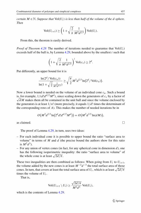
Combinatorial diameter of polytopes and simplicial complexes 457
certain M ∈ N. Suppose that Vol(Ui) is less than half of the volume of the d-sphere.Then
Vol(Ui+1) ≥(
1 +√
2
π
1
M2d2.5
)Vol(Ui).
From this, the theorem is easily derived.
Proof of Theorem 4.28 The number of iterations needed to guarantee that Vol(Ui)
exceeds half of the ball is, by Lemma 4.29, bounded above by the smallest i such that
(1 +
√2
π
1
M2d2.5
)i
Vol(cv) ≥ 2d .
Put differently, an upper bound for it is
ln(2d/Vol(cu))
ln(1 +√
2π
1M2d2.5 )
≥√
π
2M2d2.5 ln
(2d/Vol(cu)
).
Now a lower bound is needed on the volume of an individual cone cu. Such a boundis, for example, 1/(d!dd/2Md), since scaling down the generators of cv by a factor of√
dM makes them all be contained in the unit ball and since the volume enclosed bythe generators is at least 1/n! (more precisely, it equals 1/d! times the determinant ofthe corresponding rows of A). This makes the number of needed iterations be in
O(M2d2.5 ln
(2dd!dd/2Md
)) = O(M2d3.5 ln(dM)
),
as claimed. �
The proof of Lemma 4.29, in turn, uses two ideas:
– For each individual cone it is possible to upper bound the ratio “surface area tovolume” in terms of M and d (the precise bound the authors show for this ratiois M2d3).
– For any union of vertex cones (in fact, for any spherical cone in dimension d), onehas the following isoperimetric inequality: the ratio “surface area to volume” ofthe whole cone is at least
√2d/π .
These two inequalities are then combined as follows: When going from Ui to Ui+1,the volume added by the new cones is at least M−2d−3 the total surface area of thosecones. In turn, that covers at least the total surface area of Ui , which is at least
√2d/π
times the volume of Ui .That is,
Vol(Ui+1 \ Ui) ≥√
2d/π
M2d3Vol(Ui),
which is the contents of Lemma 4.29.
458 F. Santos
5 Conclusion
This paper deals with the problem of bounding the diameter of polyhedra in termsof their dimension and number of facets. The last section of the paper revises re-cent progress (sometimes “negative progress,” as in the case of the counterexamplesto the Hirsch Conjecture) but most of the paper (Sects. 2 and 3) is devoted to at-tempts at “proving it by generalizing it.” For this, the diameter problem on simplicialcomplexes is posed and studied without assuming that the complexes come from apolytope or polyhedron.
The main conclusion is that without extra conditions on the complexes polynomialbounds simply do not exist (Corollary 2.12). However, several results hint that thereis hope of getting polynomial bounds under the mild assumption of the complexesbeing normal, a.k.a. locally strongly connected. For example, Conjecture 3.4 wouldimply this by Proposition 3.7.
So, perhaps the main question is how plausible Conjecture 3.4 is. I have to admitthat, although 2 years ago I was very optimistic about this conjecture, now I havedoubts. Let me explain why. For me, the strongest evidence in favor of Conjecture 3.4is the combination of Examples 3.8 and 3.9 and Proposition 3.10. The examples showtwo extremal and “opposite” families of (multi)complexes for which the conjectureholds and, what is more striking, for which the bound in the conjecture is sharp. Whatnow makes me have doubts is the realization that these two examples are particularcases (in the “connected layer family” world) of flag and normal (multi)complexes.And for flag and normal complexes, we actually know the Hirsch bound to hold(Theorem 4.12).
In the other direction, the arguments of Sect. 4.2 indicate that we need new ideasif we want to have non-Hirsch polytopes that break the “linear barrier.” Even theconstruction of polytopes (or pure, normal simplicial complexes, for that matter) withdiameter exceeding 2n seems an extremely ambitious goal at this point.
Acknowledgements I would very much like to thank the two editors of TOP, Miguel Ángel Goberna andJesús Artalejo, for the invitation to write this paper. Unfortunately, while the paper was being processed,I received the extremely sad news of the passing away of Jesús. Let me send my warmest condolences tohis colleagues, friends, and above all, his family.
I also want to thank Jesús De Loera, Steve Klee, Tamás Terlaky, and Miguel Ángel Goberna (again)for sending me comments and typos on the first version of the paper.
References
Adiprasito K, Benedetti B (2013, preprint) The Hirsch bound holds for normal flag complexes. http://arxiv.org/abs/1303.3598
Adler I, Dantzig GB (1974) Maximum diameter of abstract polytopes. Math Program Stud 1:20–40. Piv-oting and extensions
Altshuler A, Bokowski J, Steinberg L (1980) The classification of simplicial 3-spheres with nine verticesinto polytopes and non-polytopes. Discrete Math 31:115–124
Barnette D (1974) An upper bound for the diameter of a polytope. Discrete Math 10:9–13Betke U (2004) Relaxation, new combinatorial and polynomial algorithms for the linear feasibility prob-
lem. Discrete Comput Geom 32(3):317–338Bonifas N, Di Summa M, Eisenbrand F, Hähnle N, Niemeier M (2012) On sub-determinants and the diam-
eter of polyhedra. In: Proceedings of the 28th annual ACM symposium on computational geometry,SoCG’12, pp 357–362
Combinatorial diameter of polytopes and simplicial complexes 459
Bremner D, Deza A, Hua W, Schewe L (2013) More bounds on the diameter of convex polytopes. OptimMethods Softw 28(3):442–450. Special issue in honour of Professor Kees Roos’70th Birthday
Bremner D, Schewe L (2011) Edge-graph diameter bounds for convex polytopes with few facets. ExpMath 20(3):229–237
Chubanov S (2012) A strongly polynomial algorithm for linear systems having a binary solution. MathProgram 134(2):533–570
Dantzig GB (1951) Maximization of a linear function of variables subject to linear inequalities. In: Activ-ity analysis of production and allocation, cowles commission monograph no. 13. Wiley, New York,pp 339–347
Dantzig GB (1963) Linear programming and extensions. Princeton University Press, PrincetonDe Loera JA (2011) New insights into the complexity and geometry of linear optimization. In: Optima,
mathematical optimization society newsletter, vol 87, pp 1–13De Loera JA, Klee S (2012) Transportation problems and simplicial polytopes that are not weakly vertex-
decomposable. Math Oper Res 37(4):670–674De Loera JA, Rambau J, Santos F (2010) Triangulations: structures for algorithms and applications. Algo-
rithms and computation in mathematics, vol 25. Springer, BerlinDeza A, Terlaky T, Zinchenko Y (2008) Polytopes and arrangements: diameter and curvature. Oper Res
Lett 36(2):215–222Deza A, Terlaky T, Zinchenko Y (2009a) Central path curvature and iteration-complexity for redundant
Klee–Minty cubes. Adv Appl Math Mech 17:223–256Deza A, Terlaky T, Zinchenko Y (2009b) A continuous d-step conjecture for polytopes. Discrete Comput
Geom 41:318–327Dongarra J, Sullivan F (2000) Guest editors’ introduction: the top 10 algorithms. Comput Sci Eng 2(22):2
pagesDunagan J, Spielman DA, Teng S-H (2011) Smoothed analysis of condition numbers and complexity
implications for linear programming. Math Program, Ser A 126(2):315–350Dunagan J, Vempala S (2008) A simple polynomial-time rescaling algorithm for solving linear programs.
Math Program, Ser A 114(1):101–114Dyer M, Frieze A (1994) Random walks, totally unimodular matrices, and a randomised dual simplex
algorithm. Math Program 64:1–16Eisenbrand F, Hähnle N, Razborov A, Rothvoß T (2010) Diameter of polyhedra: limits of abstraction.
Math Oper Res 35(4):786–794Friedmann O (2011) A subexponential lower bound for Zadeh’s pivoting rule for solving linear programs
and games. In: Proceedings of the 15th conference on Integer Programming and Combinatorial Op-timization, IPCO’11, New York, NY, USA
Friedmann O, Hansen T, Zwick U (2011) Subexponential lower bounds for randomized pivoting rulesfor the simplex algorithm. In: Proceedings of the 43rd ACM symposium on theory of computing,STOC’11, San Jose, CA, USA
Goodey PR (1972) Some upper bounds for the diameters of convex polytopes. Isr J Math 11:380–385Gromov M (1987) Hyperbolic groups. In: Essays in group theory. Math sci res inst publ, vol 8. Springer,
New York, pp 75–263Hähnle N (2012, preprint) Constructing subset partition graphs with strong adjacency and end-point count
properties. arXiv:1203.1525Hähnle N, Klee S, Pilaud V (2013) Obstructions to weak decomposability for simplicial polytopes. Proc
Amer Math Soc. To appear. http://arxiv.org/abs/1206.6143Holton DA, Sheehan J (1993) The Petersen graph. Australian mathematical society lecture series, vol 7.
Cambridge University Press, CambridgeIzmestiev I, Joswig M (2003) Branched coverings, triangulations, and 3-manifolds. Adv Geom 3(2):191–
225Kalai G (1992) Upper bounds for the diameter and height of graphs of convex polyhedra. Discrete Comput
Geom 8(4):363–372Kalai G (coordinator) (2010) Polymath 3: polynomial Hirsch Conjecture. http://gilkalai.wordpress.com/
2010/09/29/polymath-3-polynomial-hirsch-conjectureKalai G, Kleitman DJ (1992) A quasi-polynomial bound for the diameter of graphs of polyhedra. Bull Am
Math Soc 26:315–316Karmarkar N (1984) A new polynomial-time algorithm for linear programming. Combinatorica 4:373–
395Khaachiyan LG (1979) A polynomial algorithm in linear programming. Dokl Akad Nauk SSSR 244:1093–
1096
460 F. Santos
Kim ED (2013) Polyhedral graph abstractions and an approach to the Linear Hirsch Conjecture. MathProgram, Ser A. To appear. http://arxiv.org/abs/1103.3362v1
Kim ED, Santos F (2009, unpublished manuscript) Companion to “An update on the Hirsch Conjecture”.22 pages. http://arxiv.org/abs/0912.4235
Kim ED, Santos F (2010) An update on the Hirsch Conjecture. Jahresber Dtsch Math-Ver 112(2):73–98Klee V (1964) Diameters of polyhedral graphs. Can J Math 16:602–614Klee V (1966) Paths on polyhedra II. Pac J Math 17(2):249–262Klee V, Kleinschmidt P (1987) The d-step conjecture and its relatives. Math Oper Res 12(4):718–755Klee V, Minty GJ (1972) How good is the simplex algorithm? In: Inequalities, III, Proc third sympos,
Univ. California, Los Angeles, Calif., 1969 Academic Press, New York, pp 159–175. Dedicated tothe memory of Theodore S Motzkin
Klee V, Walkup DW (1967) The d-step conjecture for polyhedra of dimension d < 6. Acta Math 133:53–78
Kleinschmidt P, Onn S (1992) On the diameter of convex polytopes. Discrete Math 102(1):75–77Larman DG (1970) Paths on polytopes. Proc Lond Math Soc 20(3):161–178Matschke B, Santos F, Weibel C (2012, preprint) The width of 5-prismatoids. 28 pages. http://arxiv.org/
abs/1202.4701Naddef D (1989) The Hirsch conjecture is true for (0,1)-polytopes. Math Program 45:109–110Nash JC (2000) The (Dantzig) simplex method for linear programming. Comput Sci Eng 2(29):3 pagesProvan JS, Billera LJ (1980) Decompositions of simplicial complexes related to diameters of convex poly-
hedra. Math Oper Res 5(4):576–594Santos F (2012) A counter-example to the Hirsch Conjecture. Ann Math (2) 176:383–412Santos F, Stephen T, Thomas H (2012) Embedding a pair of graphs in a surface, and the width of 4-
dimensional prismatoids. Discrete Comput Geom 47(3):569–576Schewe L (2009) Non-realizable minimal vertex triangulations of surfaces: showing non-realizability using
oriented matroids and satisfiability solvers. Discrete Comput Geom 43(2):289–302Smale S (2000) Mathematical problems for the next century. In: Mathematics: frontiers and perspectives.
Am Math Soc, Providence, pp 271–294Todd MJ (1980) The monotonic bounded Hirsch Conjecture is false for dimension at least 4. Math Oper
Res 5(4):599–601Vershynin R (2009) Beyond Hirsch Conjecture: walks on random polytopes and smoothed complexity of
the simplex method. SIAM J Comput 39(2):646–678Ziegler GM (1995) Lectures on polytopes. Graduate texts in mathematics, vol 152. Springer, BerlinZiegler GM (2012) Who solved the Hirsch Conjecture? Doc Math. Extra volume: Optimization stories,
75–85


![Vašek Chvátal: A Very Short Introductionbico/papers/vasek_gc.pdf · Polytopes and a Hierarchy of Combinatorial Problems” [19]. He defined the clo-sure of a system of linear inequalities](https://static.fdocuments.in/doc/165x107/603de92f32c1c631e051f1e2/vaek-chvtal-a-very-short-introduction-bicopapersvasekgcpdf-polytopes.jpg)