Recent practices and advances for AMIS crop yield ... · recent practices and advances for amis...

Recent pRactices and advances foR aMis cRop yield foRecasting at faRM and paRcel level: A review

Recent pRactices and advances

foR aMis cRop yield foRecasting at faRM

and paRcel level: A review

FOOD AND AGRICULTURE ORGANIZATION OF THE UNITED NATIONS

Rome, 2017

Recent pRactices and advances foR aMis cRop yield foRecasting at faRM and paRcel level: A Review ii

The designations employed and the presentation of material in this information product do not imply the expression of any opinion whatsoever on the part of the Food and Agriculture Organization of the United Nations (FAO) concerning the legal or development status of any country, territory, city or area or of its authorities, or concerning the delimitation of its frontiers or boundaries. The mention of specific companies or products of manufacturers, whether or not these have been patented, does not imply that these have been endorsed or recommended by FAO in preference to others of a similar nature that are not mentioned.

The views expressed in this information product are those of the author(s) and do not necessarily reflect the views or policies of FAO.

ISBN 978-92-5-109779-3

© FAO, 2017

FAO encourages the use, reproduction and dissemination of material in this information product. Except where otherwise indicated, material may be copied, downloaded and printed for private study, research and teaching purposes, or for use in non-commercial products or services, provided that appropriate acknowledgement of FAO as the source and copyright holder is given and that FAO’s endorsement of users’ views, products or services is not implied in any way.

All requests for translation and adaptation rights, and for resale and other commercial use rights should be made via www.fao.org/contact-us/licence-request or addressed to [email protected].

FAO information products are available on the FAO website (www.fao.org/publications) and can be purchased through [email protected].

Recommended citationDelincé, J. 2017. Recent practices and advances for AMIS crop yield forecasting at farm/parcel level: A review. FAO – AMIS Publication: Rome.

This publication has been printed using selected products and processes so as to ensure minimal environmental impact and to promote sustainable forest management.

Layout: Laura Monopoli

Cover photos: © FAO/ Jacques Delincé

© FAO/ Jacques Delincé

© FAO/Jacques Delincé

Recent pRactices and advances foR aMis cRop yield foRecasting at faRM and paRcel level: A Review iii

ContentsAcknowledgements ivAcronyms vFigures viiExecutive summary ix

Chapter 1 Introduction ............................................................................................................................................................ 1

Chapter 2 The components of the crop yield model ........................................................................ 7

Chapter 3 The main crop yield models .............................................................................................................11

Chapter 4 Uncertainty in modelling (AgMIP and MACSUR) ..................................................21

Chapter 5 Recent advances ............................................................................................................................................27

Chapter 6 Specific observations on rice, corn, wheat and soybean .............................31

Chapter 7 Role of the private sector: insurances, start-ups, industry and foundations ..............................................................................................................................................37

Chapter 8 Current recommendations .................................................................................................................41

References ..............................................................................................................................................................43

Recent pRactices and advances foR aMis cRop yield foRecasting at faRM and paRcel level: A Review iv

AcknowledgementsThis publication was prepared by Jacques Delincé, senior statistician, and Consultant for the Statistics Division (ESS) of the Food and Agriculture Organization of the United Nations (FAO).

The contributions of leading crop growth modelers – B. Wu, M. Donatelli, G. Genovese, J.P. Guerschman, J.W Jones, M. Meisner, A. Potgieter, S. Ray, O. Rojas, O. Vergara – and of FAO staff – Y. Seid, F. Fonteneau, F. Bolliger and C. Duhamel – during the preparation of this review are gratefully acknowledged. The support provided for compilation of the bibliographic material by L. Galeotti of the FAO Library was highly appreciated. Norah de Falco coordinated the design and communication aspects. The publication was edited by Sarah Pasetto.

This review complements a former 2016 AMIS publication entitled Crop Yield Forecasting: Methodological and Institutional Aspects. Current Practices from Selected Countries (Belgium, China, Morocco, South Africa, USA) with a focus on AMIS Crops (Maize, Rice, Soybeans and Wheat)”.

This publication was prepared with the financial support of the Bill & Melinda Gates Foundation, through the FAO Project MTF-GLO-359-BMG on “Strengthening agricultural market information systems globally and in selected countries, using innovative methods and digital technology”, which is implemented in the context of the G20 AMIS Initiative.

Recent pRactices and advances foR aMis cRop yield foRecasting at faRM and paRcel level: A Review v

AcronymsAGMIP The Agriculture Model Intercomparison and Improvement ProjectAMIS Agricultural Market Information SystemAPSIM Agricultural Production Systems sIMulatorAVHRR Advanced Very High Resolution RadiometerCER CO2 Exchange RateCERES Crop Environment Resource Synthesis ModelCGM Crop Growth ModelCIAT Centro Internacional de Agricultura Tropical (CGIAR)CIMSAMS Center for Integrated modeling of Sustainable Agriculture & Nutrition SecurityCNC Critical Nitrogen ConcentrationCROPSYST Cropping Systems Simulation ModelCSM Crop Simulation ModelCWSB Crop Specific Water BalanceDGVM Dynamic Global Vegetation ModelsDMP Dry Matter ProductionDSSAT Decision Support System for Agrotechnology Transfere conversion coefficient (biomass produced / intercepted radiation)ENSO-MEI El Niño Southern Oscillation Multivariate IndexEPIC Environmental Policy Integrated Climate modelESA European Space AgencyEVI Enhanced Vegetation IndexFAO Food and Agriculture OrganizationfPAR Fraction of Photosynthetic Active RadiationGCVI Green Chlorophyll Vegetation Index GDP Gross Domestic ProductGDD Growing Degree DaysGEOGLAM Global Agriculture MonitoringGEOSHARE Geospatial Open Source Hosting of Agriculture, Resource & Environmental DataGGCM Global Gridded Crop ModelGIS Geographical Information SystemGYGA Global Yield Gap AtlasICCYF Integrated Canadian Crop Yield ForecastsILSI International Life Sciences InstituteLAI Leaf Area IndexMACSUR Modeling European Agriculture with Climate Change for Food SecurityMAPE Mean Absolute Percentage ErrorMARS Monitoring Agricultural ResourceS Project (EU)MSEP Mean Square Error of PredictionNASA National Aeronautics and Space Administration (USA)NDVI Normalized Difference Vegetation IndexNEXTGEN Next Model Generation

Recent pRactices and advances foR aMis cRop yield foRecasting at faRM and paRcel level: A Review vi

NOAA National Oceanic and Atmospheric Administration (USA)PASW Plant Available Soil WaterRMSE Root Mean Square ErrorRUE Radiation Use EfficiencySALUS System Approach to Land Use SustainabilitySAR Synthetic Aperture Radar SAVI Soil Adjusted Vegetation IndexSMAP Soil Moisture Active and Passive MissionSTARS Spurring a Transformation for Agriculture through Remote SensingSTICS Simulateur mulTIdiscplinaire pour les Cultures StandardTCI Temperature Conditions IndexTE Transpiration EfficiencyTGI Triangular Greenness IndexUSDA PSD United States Department of Agriculture, Production & Supply DatabaseWOFOST WOrld FOod Studies Model

Recent pRactices and advances foR aMis cRop yield foRecasting at faRM and paRcel level: A Review vii

FiguresFigure 1. Evolution of Yield for Wheat, Corn, Soybean and Rice in selected regions (1995–2016) .......................................................................................................................3Figure 2. Evolution of World Productions (Mtonnes) and Areas (Mha) ...................................................4Figure 3. IGC Grains and Oilseeds Index and sub-Indices (Daily) ...............................................................4Figure 4. The various modeling levels From potential to actual yields, the various modeling levels ................................................................................................................................6Figure 5. Key attributes of crop growth simulation models ..........................................................................13Figure 6. Diagram of the components of the SALUS model .......................................................................15Figure 7. External models integrated into the APSIM system since its introduction .............16Figure 8. Applications of Remote Sensing in Agriculture ................................................................................17Figure 9. Average Global Gridded Crop Model (GGCM) maize yield (rescaled to the common global average of historical yield in G) for various models from 1980 to 2010 .................................................................................................... 23Figure 10. Relative change (%) in RCP 8.5 dekadal mean production for various GGCM, from median for all GCM, with and without effects of CO2 for maize, wheat, rice and soybean ......................... 24Figure 11. List of remote sensing indices related to vegetation cover and chlorophyll content ........................................................................................................................................ 28Figure 12. Coefficient of variation of crop yields over a 30-year period for (a) maize, (b) rice, (c) wheat and (d) soybean .................................................................................... 32Figure 13. Global yield gap protocol for data aggregation ............................................................................... 35

Recent pRactices and advances foR aMis cRop yield foRecasting at faRM and paRcel level: A Review viii

Recent pRactices and advances foR aMis cRop yield foRecasting at faRM and paRcel level: A Review ix

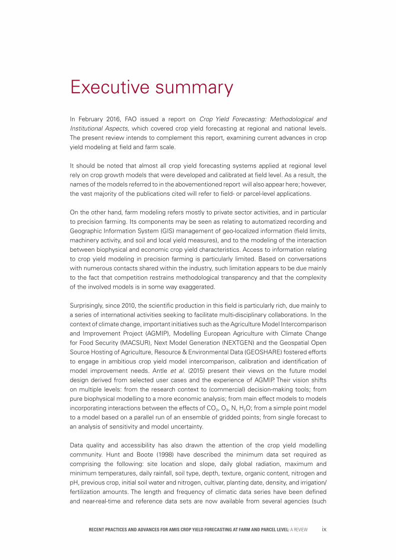
Executive summaryIn February 2016, FAO issued a report on Crop Yield Forecasting: Methodological and Institutional Aspects, which covered crop yield forecasting at regional and national levels. The present review intends to complement this report, examining current advances in crop yield modeling at field and farm scale.

It should be noted that almost all crop yield forecasting systems applied at regional level rely on crop growth models that were developed and calibrated at field level. As a result, the names of the models referred to in the abovementioned report will also appear here; however, the vast majority of the publications cited will refer to field- or parcel-level applications.

On the other hand, farm modeling refers mostly to private sector activities, and in particular to precision farming. Its components may be seen as relating to automatized recording and Geographic Information System (GIS) management of geo-localized information (field limits, machinery activity, and soil and local yield measures), and to the modeling of the interaction between biophysical and economic crop yield characteristics. Access to information relating to crop yield modeling in precision farming is particularly limited. Based on conversations with numerous contacts shared within the industry, such limitation appears to be due mainly to the fact that competition restrains methodological transparency and that the complexity of the involved models is in some way exaggerated.

Surprisingly, since 2010, the scientific production in this field is particularly rich, due mainly to a series of international activities seeking to facilitate multi-disciplinary collaborations. In the context of climate change, important initiatives such as the Agriculture Model Intercomparison and Improvement Project (AGMIP), Modelling European Agriculture with Climate Change for Food Security (MACSUR), Next Model Generation (NEXTGEN) and the Geospatial Open Source Hosting of Agriculture, Resource & Environmental Data (GEOSHARE) fostered efforts to engage in ambitious crop yield model intercomparison, calibration and identification of model improvement needs. Antle et al. (2015) present their views on the future model design derived from selected user cases and the experience of AGMIP. Their vision shifts on multiple levels: from the research context to (commercial) decision-making tools; from pure biophysical modelling to a more economic analysis; from main effect models to models incorporating interactions between the effects of CO2, O3, N, H2O; from a simple point model to a model based on a parallel run of an ensemble of gridded points; from single forecast to an analysis of sensitivity and model uncertainty.

Data quality and accessibility has also drawn the attention of the crop yield modelling community. Hunt and Boote (1998) have described the minimum data set required as comprising the following: site location and slope, daily global radiation, maximum and minimum temperatures, daily rainfall, soil type, depth, texture, organic content, nitrogen and pH, previous crop, initial soil water and nitrogen, cultivar, planting date, density, and irrigation/fertilization amounts. The length and frequency of climatic data series have been defined and near-real-time and reference data sets are now available from several agencies (such

Recent pRactices and advances foR aMis cRop yield foRecasting at faRM and paRcel level: A Review x

as the United States Geological Service or USGS, the National Oceanic and Atmospheric Administration or NOAA, the European Space Agency or ESA, and FAO), which deliver the information on soil, weather and crop masks as open access public goods. The availability of Global Positioning Services (GPS), GIS and automatic data transmission has also boosted private-sector prescriptive farming, allowing for an intra-field management of fertilization and water application that can ensure the sustainable economic use of the factors of production.

The main processes modeled in the equation system will mimic the factors limiting plant growth: soil moisture and nutrient availability, and solar radiation. The aspects of crop varieties and phenology, planting density, sowing date, rainfall distribution, fertilization plan and diseases will in turn interact with these three limiting factors, and influence the final storage organ accumulation. Considering that growth is basically dependent on the energy balance between the plant’s photosynthesis and respiration activities, the chlorophyll pigment, the enzyme activity response to the environment (temperature and water), and the light interception will be at the core of the models. Although in recent years the energy balance has not improved very much, an increase of accumulation in the storage organs has resulted, mainly due to the increase in the harvest index (the ratio of grain yield to shoot yield), reaching a level of 50 percent for wheat. The genotype characteristics of the plant are thus a compulsory component of all models.

Despite the progresses achieved in terms of model specification and data quality, much uncertainty remains. The major drawbacks of statistical models are that they tend to underperform in case of extreme events, and that the pure process-based models require a quantity of detailed information that is usually incompatible with the time and budget available for operational activities. In the projects for model intercomparison, the range of results in a set of 10–15 models is such that the current recommendation is to rely upon an ensemble solution of well-recognized models and data.

The main recent progresses for maize, wheat, rice and soybean may be found in the proceedings of the MACSUR and AGMIP projects. Most studies focused upon the simulation of crop response to changes in CO2 concentration, extreme temperatures (heat stress and frost damage), rainfall and their specificities at each development stage, tropospheric ozone concentration and pest and diseases, and crop rotations and intercropping (Müller and Eliot 2015).

Farm decision systems are now widely used in developed countries. The most popular of such systems include the following: the Climate Field View, that Monsanto claims to apply to more than 50 million ha, Yield Prophet (Australia), Agro Climate (Florida University), AgBiz (Oregon State University), and Air Worldwide (Insurance). Unfortunately, most of these systems are not open source and thus require farmers to make area-based payments. In addition, the crop yield model component seems to have been kept at a minimum level of complexity, thus making it impossible to conclude that any progress has been made, other than the industrialization of the process. The breeding sector has also identified the potential of merging crop models with genetic markers; however, in this context too, the explanation provided (general mixed linear models modelling the interaction between quantitative trait loci – QTL – and the environment) do not facilitate comprehension of the exact progress made and their potential replication.

Recent pRactices and advances foR aMis cRop yield foRecasting at faRM and paRcel level: A Review xi

The 2003 special issue of the European Journal of Agronomy on “Modeling Cropping Systems: science, software and application” and the 2015 special issue of Agricultural System, titled “Towards a New Generation of Agricultural System Models, Data, and Knowledge Products” assessed the progresses made over the last 10 years on crop yield modeling and advocated a recommended direction of move. Likewise, it may be expected that a new generation of modelers will in due time issue a 2025 review issue, showing that the current projects have evolved into reality and proposing new goals.

Recent pRactices and advances foR aMis cRop yield foRecasting at faRM and paRcel level: A Review xii

Recent pRactices and advances foR aMis cRop yield foRecasting at faRM and paRcel level: A Review 1

1IntroductionIn most countries, although the proportion of national GDP constituted by the agricultural sector has been declining for decades, the forecasting of food production remains a major challenge for all the economic actors of modern societies. At all levels – government, industry, farm, household – decisions must be taken on the basis of advanced knowledge of the potential influence of economic, biotic and abiotic factors upon crop yields of the major food commodities, especially the four major crops constituting the priorities of the Agricultural Market Information System (AMIS), the significance of which is clear from Table 1 below:

• Corn, with a harvested area of 177 million ha, a production of 959 million tonnes and exports for only 140 million tonnes;

• Wheat, with 225 million ha, 735 million tonnes and 173 million tonnes respectively; • Rice, with 160 million ha, 472 million tonnes and 41 million tonnes; and • Soybean, with 120 million ha, 313 million tonnes, 133 million tonnes. (area/

production/exports in 2015, source USDA PSD).

Table 1. Illustration of significance of AMIS crops for the year 2015

AMIS Crop

Harvested area (million tonnes)

Production (million tonnes)

Exports (million tonnes)

Corn 177 959 140

Wheat 225 735 173

Rice 160 472 41

Soybean 120 313 133

Source: USDA PSD.


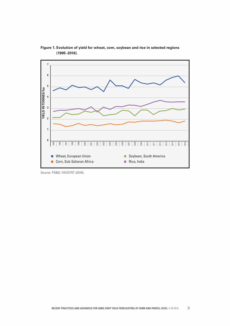
As is clear from Figures 1 to 3 below, since 1995, the world production of these commodities has followed a positive linear trend, largely explained by increases of the sown areas (10 percent for wheat and rice, 25 percent for corn and 50 percent for soybean). As studied by Potgieter et al. (2016), in Australia (a major player in cereals exports), over the last 30 years, yield increases remained limited for major cereal crops such as wheat, maize and rice (remaining at 1.2 percent yearly for wheat, representing an increase of only 21 kg/ha per year) compared to sorghum (which increased by 2.1 percent, or 44 kg/ha per year). Although the inter-annual variability of world production remained limited, with standard deviations of 1 percent for rice, 2 percent for wheat and corn and 4 percent for soybean, at the same time, the prices changed by a 1:4 ratio (compared to wheat and rice in 2008/2009). The vital character of food commodities, coupled with the limited stocks, largely explains the price volatility observed (in 2008, the low ending stocks were 169 million tonnes for wheat and 97 million tonnes for rice) and the erratic behavior of economic agents in light of the lack of information.

In reaction to these phenomena, at the 2011 G20 summit, the ministers of agriculture decided to launch AMIS1, an inter-agency platform tasked with enhancing food market transparency and encouraging the coordination of policy action in response to market uncertainty. At the same time, the private sector started to become active. The Bill & Melinda Gates Foundation invested in the monitoring of agricultural production, by introducing a change in data collection and analyses methods (Global Strategy for improving Agricultural and Rural Statistics2) and by supporting technical advances in modelling (the NEXTGEN project) and the use of new technologies (the Spurring a Transformation for Agriculture through Remote Sensing project, or STARS3). The food industry also began to model food production, aiming to make a joint academic, administration and industry effort for the purpose of Assessing Sustainable Nutrition Security (ILSI/CIMSANS; see Acharya et al., 2014).

1 http://www.amis-outlook.org/amis-about/en/.2 http://gsars.org/en/.3 http://www.stars-project.org/en/.


Figure 1. Evolution of yield for wheat, corn, soybean and rice in selected regions (1995–2016).

Source: PS&D, FAOSTAT (2016).

1995

1996

1997

1998

1999

2000

2001

2002

2003

2004

2005

2006

2007

2008

2009

2010

2011

2012

2013

2014

2015

2016

7

6

5

4

3

2

1

0

YIE

LD IN

TO

NN

ES

/ha

Wheat, European Union Corn, Sub-Saharan Africa

Soybean, South America Rice, India


Figure 2. Evolution of world productions (Mtonnes) and areas (Mha).

Source: PS&D, FAOSTAT (2016).

Figure 3. IGC Grains and Oilseeds Index and sub-indices (daily).

Source: International Grains Council (IGC).

1995

1996

1997

1998

1999

2000

2001

2002

2003

2004

2005

2006

2007

2008

2009

2010

2011

2012

2013

2014

2015

2016

1200

1000

800

600

400

200

0

250

200

150

100

50

0

PR

OD

UC

TIO

NS

AR

EA

S

Wheat production Corn production Soybean production Rice production

Wheat area Corn area Soybean area Rice area

Grains and Oilseeds Index Wheat

Maize Rice

Soybeans


In addition, the academic sector launched supranational initiatives of model comparison and improvement, namely AgMIP 4 and MACSUR 5.

Finally, start-up companies entered the field, providing alternative sources of information or a wholly new type of service. Opting to use microsatellites, companies such as Planet, TerraBella, Satellogic and Blacksky Global offer very high-resolution imagery at a very high time frequency. At the other end of the chain, precision farming agriculture has developed a range of services, such as field management advice based on meteorological and image (including drone) information.

However, grain production has two components: the yield and the area. For yield estimation, the most logic method is to proceed to field cutting. However, in addition to its high costs, this method requires waiting for crop maturity, a factor that often delays data availability. Therefore, yield forecasting relies mainly on models calibrated on the field measurements performed in previous years. However, once models rely on remotely sensed imagery, the crop locations of the current year will be required, either as crop-specific masks (which is difficult due to crop rotations), cropland masks (as in ESA’s SEN2 Africa product), or through yield correlation at pixel level (Kastens et al., 2005). The special issue of the Remote Sensing journal focusing on “Global Cropland” reviews this issue in detail (Thenkabail, 2010).

Yield forecast thus remains one of the major priorities for field managers and policymakers. Timeliness of information is of the greatest importance at field and national levels (at the former, the incorrect treatment of disease in due time can be devastating; at the latter, arranging for food imports before a crisis is less costly than obtaining emergency food assistance). Bias and the precision of forecasts are often considered from a “softer” point of view and the notion of root mean square error (RMSE) of the prediction (Wallach, 2016) is often the only criterion against which models are evaluated.

Before examining the subject matter of this review in detail, it appears relevant to clarify the following definitions, which will appear recurrently in the text:

• Yield potential (Yp): the yield of an adapted crop cultivar as determined by solar radiation, temperature, carbon dioxide, and genetic traits that govern the length of growing period, light interception by the crop canopy and its conversion to biomass, and the partition of biomass to the harvestable organs.

• Water-limited yield potential (Yw) is determined by the factors seen above and by water supply amount and distribution during the crop growth period, as well as by field and soil properties that affect soil water availability, such as slope, plant-available soil water-holding capacity, and depth of root zone.

• Actual yield (Ya): the potential yield minus the yield gap due to limiting factors caused by non-optimal management (poor sowing dates, lack of nutrients), environmental factors (temperatures) and abiotic factors such as weeds and pests. Actual yield is usually the yield provided by national statistical systems.

4 http://www.agmip.org/.5 http://macsur.eu/index.php.


• Relative yield (Y%): the ratio of Ya to Yw expressed as a percentage. This is a useful indicator of production as a function of potential. A Y% of 80 percent is regarded to fall within the upper range of wheat yields consistently achieved by leading farmers over a number of seasons.

• Exploitable yield: the additional yield that would be harvested if 80 percent of Yw is achieved (Exploitable yield = ((Yw × 0.8) − Ya)), with economic and climatic uncertainties constraining yields to fall within this range (Lobell et al., 2009).

Figure 4. From potential to actual yields: the various modelling levels.

Source: Van Ittersum et al. 2013.

POTENTIAL (Yp)

WATER-LIMITED (Yw)

WATER- ANDNUTRIENTS-LIMITED

ACTUAL (Ya)

PRODUCTION LEVEL (Mg/ha)

YIELD POTENTIAL (Yp or Yw)

EXPLOITABLEYIELD

AVERAGE FARM YIELD

(Ya)

PR

OD

UC

TIO

N S

ITU

AT

ION

YIE

LD L

EV

EL

DEFININGfactors

LIMITINGfactors

LIMITINGfactors

REDUCINGfactors

CO2

RadiationTemperature

Cultivar features

Water

WaterNutrients

WeedsPests and diseases

Pollutants

A

B

Determided by:radiation,

temperature,planting date,

cultivar maturity

(and water supply for Yw)

80%of Yp or Yw

Exploitable yieldgap


The components of the crop yield model Rana (2014) recently reviewed the advances made in crop growth and productivity. Soil moisture and nutrient availability are the first factors limiting growth, followed by solar radiation. Crop varieties and phenology, planting density, sowing date, rainfall distribution, the fertilization plan and any diseases will each interact with these three limiting factors and influence the final storage organ accumulation.

It should be recalled that growth is basically dependent upon the energy balance between the plant’s photosynthesis and respiration activities:

• Chlorophyll is at the core of photosynthesis. Composed of four ions of nitrogen and one of magnesium (C55H72O5N4Mg), its concentration in the leaves will depend on the availability of these nutrients. Last but not least, phosphorus will be also essential as ensuring intra-cell energy transfers.

• The temperature will influence enzyme activity during the Calvin cycle of photosynthesis, thus influencing the rate of CO2 absorption. Each plant species has a specific optimal temperature range, which varies among C3 and C4 plants. For the former, which include wheat, rice, soybean and sugar beet and constitute 85 percent of land plants, the optimal range is 25–30°C; for the latter, which comprise maize, sorghum, millet and sugarcane, and compose only 3 percent of plants, the optimal temperature is 35°C, due to their lower photorespiration level.

• The intercepted light will provide the energy required in the first phase of photosynthesis. Plant chlorophyll is most receptive to blue light (always associated with red light), because the blue wavelength provides the greatest intensity (ultraviolet and infrared waves being filtered by the atmosphere) and energy content (which is greater at short wavelengths) in the solar spectrum. Although 95 percent of the intercepted light will be lost due to heat regulation by transpiration, light is rarely the limiting factor, even though exceptional cases may occur: in June 2016,

2


the scarce sunlight reduced cereals yield by approximately 20 percent in central Europe.

• Water is necessary to ensure plant turgidity (structural stability), transpiration (heat emission) and photosynthesis (energy production); however, the quantity required for photosynthesis is marginal, such that water deficiency may be expected to have only indirect effects: enzyme efficiency is hampered by dehydration and stomata closure limits the availability of CO2.

• O2 and CO2 are a priori at a constant concentration in the atmosphere (even though their concentrations reduce with altitude); however, CO2 must penetrate the plant through the leaves’ stomata (which open or close in function of temperature and water availability), whereas O2 can pass through the cuticle layer. In addition, C3 and C4 plants differ in their use efficiency of CO2, with C4 plants again displaying greater efficiency.

The energy balance will result from the equilibrium between: • the glucose production of photosynthesis in the leaf’s chloroplast [H2O + sunlight O2 (waste) + ATP + NADPH + CO2 ADP + P + NADP + glucose (for efficient energy transport)] and

• the glucose consumption during cell respiration (in the mitochondria), which requires the small ATP’s energy content (C6H12O6 +O2 CO2+H2O+ ATP).

This may lead to a potential positive balance for growth and storage.

Considering a fixed value for the maximum light-saturated CO2 exchange rate per unit leaf area (CER), it may be seen that one should achieve, as rapidly as possible, the maximum leaf area index (LAI) compatible with the light intensity to reach the maximum possible assimilation, which in turn enables the maximum sink storage possible. Therefore, nutrients also have an important role to play in enabling the use of the available energy to achieve plant growth. Finally, the conversion coefficient e, defined as the quantity of biomass produced per unit of intercepted radiation, provides a measure of the efficiency with which the captured radiation is used to produce new plant material. In the absence of stress, e typically ranges between 1.0 and 1.5 g MJ–1 for C3 species in temperate environments, 1.5 to 1.7 g MJ–1 for tropical C3 species, and up to 2.5 g MJ–1 for tropical C4 species.

Although the energy balance has improved little in recent years, the growth in the accumulation in the storage organs may be ascribed mainly to the increase in the harvest index (ratio of grain yield and shoot yield), which has now reached 50 percent for wheat.

Bearing the above processes in mind, it is necessary to consider that plant growth will consist of successive development stages following a sigmoid function and that the influence of the limiting factors (temperature, water, nutrients, light, diseases) will be stage-dependent. As an example, a low photosynthesis activity at the grain-filling stage may be compensated by a mobilization of the stem sugar reserves, as occurs e.g. for wheat and sorghum. The determination of the occurrence of the individual development stages is usually based on the notion of Growing Degree Days (GDDs). These are defined as the number of mean temperature degrees above a certain threshold base temperature (which is crop specific: 5.5°C for wheat and barley, and 10°C for corn, soybean and rice) accumulated on a daily basis over a given


period of time. For cereals, the sequential stages are the following: leaf development, tillering, stem elongation, booting, heading, flowering, development of fruit, ripening and senescence.

Functional/empirical models are an elegant compromise between the demanding process-based model and the light statistical models (Basso et al., 2013). Through simple relations, major physiological processes may be approximated. The first category of models will predict the potential yield (in greenhouse conditions) based on temperature, radiation, CO2 and crop specificities, such as its phenology and biomass partitioning. More complex models will forecast the water/nutrient production by inserting equations simulating soil water, nitrogen, and carbon dynamics. Rare are the models capable of simulating the actual yield incorporating the reduction of yield due to pests, diseases or weeds. The Decision Support System for Agrotechnology Transfer (DSSAT) is capable, to some extent, of modelling pests and diseases, whereas the Agricultural Production Systems Simulator (APSIM) can also to model intercropping.


Main crop yield modelsReaders interested in the history of modelling agricultural systems should refer to Jones et al. (2016). Over the last five decades, research teams have produced hundreds of crop models differentiated by the crops covered, the targeted regions, the temporal and spatial scales, the approach (statistical or process-based), the input data required and the output variables (e.g. potential or actual yield, biomass and vegetation indices). Di Paola et al. (2016) reviewed approximately 70 models, classifying them in terms of model type, submodels, scale and time paths, crops addressed, place of application and IT system used. Most models were developed for field-level simulations and their actual use at regional or national levels often raises doubts as to their accuracy and data needs (Morell et al., 2016).

Model classification may rely on the purpose for which the model was developed. Such purpose may be the scientific understanding of crop growth (mechanistic or functional/empirical models) or the provision of support to decision making processes (predictive or descriptive models responding to external drivers). The modeling approaches separate statistical models (which build current predictions on the basis of past experience) from dynamic simulation models (which describe the effect of changes in weather or management practices). The spatial and temporal scales are the third criterion against which to differentiate models. In terms of space, the scale may range from field scale (point models with homogeneous conditions within field) to regional scale; as for time, the scale ranges from hourly steps (for pest management processes) to ten-daily steps (for delivering seasonal yield predictions). The major crop models currently in use are APSIM, the Cropping Systems Simulation model (CROPSYST), DSSAT, the Environmental Policy Integrated Climate model (EPIC), ORYZA (from the Latin word for rice), the Simulateur Multidiscplinaire pour les Cultures Standard (STICS), and the World Food Studies Model (WOFOST).

Considering the Global Gridded Crop Model Intercomparison project (Eliot et al., 2015; Rosenzweig et al., 2014), it is possible to identify the current main crop modeling systems selected by the AGMIP community for wheat, maize, soybean and rice.

3


In AGMIP Phase 1, three types of models are available: • Site-based process models (Elliot and Müller, 2015) are biophysical crop growth

field-scale models that are applied globally on a grid of points. They rely upon a detailed calibration of the crop growth processes, which requires a huge quantity of information on cultivars, management choices and soil inputs. The site-based process models used by the AGMIP community are DSSAT, EPIC and APSIM.

• Empirical or process-based models are large-area-scale models that are hybrid in the sense that they are not fully process-based. Indeed, some functional equations (i.e. management and inputs) are replaced with empirical calibration, to simplify the computations. They were developed to specifically simulate crop production at continental scale. The models used are PEGASUS (Predicting Ecosystem Goods And Services Using Scenarios), Global Agricultural Monitoring (GLAM), WOFOST-CGMS, PRYSBI-2 (Process-based Regional Yield Simulator with Bayesian Inference).

• Dynamic Global Vegetation Models (DGVMs) are used mainly to simulate the effects of future climate change on natural vegetation and its carbon and water cycles. DGVMs, which appeared in the mid-1990s, commonly simulate a variety of plant and soil physiological processes – such as the plant’s functional type, photosynthesis, competition for light-water-nitrogen, air temperature and solar radiation – and derive plant-specific indices, such as net primary production, soil-available water, root zone water supply, LAI, potential evapotranspiration, total live vegetation carbon, plant/crop establishment and mortality. Crop yields are usually not the prime focus of these models. DGVMs work at various time steps, ranging from hour to month or even year. Simulations usually run across a range of spatial scales and are carried out for thousands of “cells”, which are assumed to present homogeneous conditions. The DGVMs used under AGMIP are LPJmL (Lund-Postdam-Jena managed Land), Orchidee-crop, LPJ-GUESS (Lund-Potsdam-Jena General Ecosystem Simulator), CLM-Crop (Community Land Model – Crop)), ISAM (Integrated Science Assessment Model) and DLEM-Ag (Dynamic Land Ecosystem Model-Agriculture).

Following Basso et al. 2014, the approaches to yield forecasting will be divided into three categories: (1) crop simulation models, (2) remote sensing forecast and (3) statistical models that use the outputs produced under the first two approaches as explanatory variables.

3.1 Crop simulation models

Crop simulation models seek to predict field-scale crop yield in function of crop variety specificities, soil and weather conditions and management practice. They usually require site-specific detailed information, in function of the model’s complexity. Renowned examples of such models are DSSAT (United States of America) and APSIM (Australia). Although stochastic models do exist to introduce uncertainty into the input data, most of the current decision-making models are deterministic.

The minimum data set required is described by Hunt and Boote (1998) as comprising


the following: site location and slope, daily global radiation, maximum and minimum temperatures, daily rainfall, soil type, depth, texture, organic content, nitrogen and pH levels, previous crop(s), initial soil water and nitrogen, cultivar, planting date, density, and irrigation/fertilization amounts. More recently, Grassini et al. (2015) examine the issue of the data requirements for reliable crop modeling in the United States of America, Argentina and Kenya. For weather data, they conclude that between 10 and 20 years of archived information are necessary in function of the difficulties that may be posed by the sites (i.e. initial data quality and level of inter-annual variability) to maintain the yield estimates within +/- 10 percent of the estimations based on 30 years. The authors consider that data measured on a daily basis at least are required for pluviometry and temperature (Tmin, Tmax). With the exception of wind speed, the other variables (solar radiation and vapour pressure) necessary to calculate evapotranspiration can be derived or retrieved from data sets such as NASA-POWER. Cropping system details are also required (sowing dates, crop sequence in case of multiple-year cropping, irrigated or rain-fed cultivation, the GDDs between sowing and grain maturity for recent cultivars, and plant density). Usually, these must be derived from ancillary data. Soil information comprises mainly slope, drainage, soil depth and texture classes (for soil water capacity – the Plant Available Soil Water, or PASW).

Van Ittersum et al. (2013) insist that models must be rigorously evaluated for their ability to reproduce measured yields of field crops that have received near-optimal management practices, across a wide range of environments and management practices. They summarize the key attributes of crop growth simulation models as shown in Figure 5.

Figure 5. Key attributes of crop growth simulation models.

DESIRED ATTRIBUTES OF CROP SIMULATION MODELS

Desired attributes Explanation

Daily step simulationSimulation of daily crop growth and development based on weather, soil, and crop physiological attributes

Flexibility to simulate management practices Key management practices include: sowing date, plant density, cultivar maturity

Simulation of fundamental physiological processesSimulation of key physiological processes such as crop development, net carbon assimilation, biomass partitioning, crop water relations, and grain growth

Crop specificity

Should reflect crop-specific physiological attributes for respiration and photosynthesis, critical stages and growth periods that define vegetative and grain filling periods, and canopy architecture

Minimum requirement of crop ‘genetic’ coefficientsThe model should have a low requirement of crop-site ‘genetic’ coefficients, preferably only a limited number of phenological coefficients


DESIRED ATTRIBUTES OF CROP SIMULATION MODELS

Desired attributes Explanation

Validation against data from field crops that approach Yp and Yw

Comparison of model outcomes (grain yield, aboveground dry matter, crop evapotranspiration) against actual measured data from field crops that received management practice conductive to achieve Yp (irrigated) or Yw (rainfed crops)

User friendly

Models embedded in user-friendly interfaces, where required data inputs and outputs can be easily visualized, and with flexbility to modify defalut values for internal parameters

Full documentation of model parameterization and availability

Publicly available models, published in the peer-review literature, with full documentation and publicly available code, and with reference to data sources for internal parameter values

Source: Van Ittersum et al. 2013.

As examples of Crop Simulation Models (CSM), the following sections elaborate upon the presentation of Ritchie’s System Approach to Land Use Sustainability (SALUS) model1 and on the paper by Holzworth et al. (2014) on the evolution of the APSIM model. These two models represent simple and complex cases respectively.

The SALUS model should be considered as a simplified version of the DSSAT. Among other uses, it enables simulations for wheat, maize, soybean and rice. The SALUS simulation system is designed to model continuous crop, soil, water and nutrient conditions under different management strategies for multiple years. These strategies may present various crop rotations, planting dates, plant populations, irrigation and fertilizer applications, and tillage regimes. The program simulates plant growth and soil conditions every day (during growing seasons and fallow periods) for any time period, when weather sequences are available. For any simulation run, a number of different management strategies can be run simultaneously. Every day, and for each management strategy being run, all major components of the crop-soil-water model are executed. These components are: management practices, water balance, soil organic matter, nitrogen and phosphorous dynamics, heat balance, plant growth and plant development. The water balance considers surface runoff, infiltration, surface evaporation, saturated and unsaturated soil water flow, drainage, root water uptake, soil evaporation and transpiration. The soil organic matter and nutrient model simulates organic matter decomposition, nitrogen mineralization and formation of ammonium and nitrate, nitrogen immobilization, gaseous nitrogen losses and three pools of phosphorus. The development and growth of plants considers the environmental conditions (particularly temperature and light) to calculate the plant’s potential rates of growth. This growth is then reduced on the basis of water and nitrogen limitations.

1 http://nowlin.psm.msu.edu/salus/overview.html.


Figure 6. Diagram of the components of the SALUS model.

Source: J.T. Ritchie.

The biophysical model consists of three main structural components: a. A set of crop growth modules (derived mainly from the Crop Environment

Resource Synthesis (CERES) model. Phasic development is controlled by environmental variables (e.g. degree days and photoperiod), which are governed by variety-specific genetic coefficients. Dry matter production (DMP) is a function of the potential rates (controlled by solar radiation and parameters defining the variety-specific growth potential), which are then reduced according to water and nitrogen limitations.

b. A soil organic matter and nutrient (nitrogen, phosphorus) cycling module. The main external inputs required by this module are: soil texture, bulk density, horizon depths, total organic carbon and nitrogen, and initial mineral nitrogen content.

c. A soil water balance and temperature module incorporating a time-to-ponding (TP) concept to replace the previous CERES runoff and infiltration calculations. The main management-influenced parameter controlling the TP curve is the saturated hydraulic conductivity at the soil surface, which varies as a function of tillage, soil compaction and surface residue amounts. This approach requires additional information regarding rainfall intensity.

For pest and diseases, the SALUS model interfaces with external models of pest dynamics and damages, incorporating results such as reduction in plant number, photosynthetic rate reduction, leaf senescence acceleration, tissue consumption and turgor reduction.

The Agricultural Production System Simulator (APSIM) is a complex but free-access (for non-commercial use) framework for modelling farming systems developed in Australia. Its plant models simulate the key physiological processes, including phenology, organ (leaf, stem, root and grain) development, water and nutrient uptake, carbon assimilation, biomass

crops ■ Wheat ■ Barley ■ Maize ■ Soybean ■ Potato ■ etc...

biotic interactions

yeld atmospheric flux

socio-economic

drainageleaching

environmental

runoffsoil erosion

roots

management ■ Crop Sequencing ■ Planting ■ Residue ■ Tillage ■ Fertilizer ■ Manure ■ Pesticide ■ Irrigation ■ Drainage

weather

soilWater balance

Carbon balanceHeat balance

Nutrient balance (N & P)


and nitrogen partitioning between organs, and responses to abiotic stresses. Thirty plant species (including arable crops, cotton, grassland, eucalyptus and oil palm) are currently covered in the Plant Modeling Framework, thus providing a library of plant organ and process submodels that can be coupled, at runtime, to construct a model in much the same way that models can be coupled to construct a simulation. This means that model developers can obtain a dynamic composition of lower-level process and organ classes (e.g. photosynthesis and leaf) into larger constructions (e.g. wheat and sorghum) without additional coding. The impact of increased atmospheric CO2 concentration upon simulated crop growth is modelled via changes to radiation use efficiency (RUE), transpiration efficiency (TE) and the critical nitrogen concentration (CNC) for crop growth. The evolution of the APSIM model since 1990 is schematically reproduced in Figure 7.

Figure 7. External models integrated into the APSIM system since its introduction.

Source: Holzworth et al. 2014.

Its soil models simulate the relevant processes occurring on and within the soil profile; these includes water infiltration and movement, evaporation, runoff and drainage, temperature variations, the cycling of nitrate, ammonium and other solutes (phosphorus), and soil organic matter decomposition (litter or residues).

APSIM’s animal models simulate cattle and sheep in agricultural systems, including their effects on crops and soils. Grazing of grain crops, both during the growing season and as residues, can be modelled. The return of nutrients to the soil as urine and faeces is explicitly modelled.

Coupling models together to form larger “models” and then configuring each by specifying their input parameter values construct an APSIM simulation. A large set of toolboxes of biophysical and infrastructure models provide the necessary pieces to construct a representation of a single point in space. This single soil, climate or management construct has traditionally represented a field on a farm having a uniform soil and management. Every APSIM simulation must be represented as an XML document before it can be executed. The

swim (Verburg et al., 1996b)

ausfarm

ozcot

grasp (Bell et al., 2008)

agpasture (Li et al., 2011)

oryza (Gaydon et al., 2012b)

dymex (Whish et al., 2014)

swim (Verburg et al., 1996b)

grazplan (Freer et al., 1997)

ozcot (Hearn, et al.,1994)

grasp (Ricket et al., 2000)

dairymod (Johnson et al., 2008)

oryza2000 (Bouman et al., 2012b)

dymex (Maywald et al., 2014)

apsim

apsim 7.6

1990

2014


most common way of building this document is via a graphical user interface, which enables models to be chosen from a set of toolboxes.

3.2

Remote sensing forecasts of crop yields are one of the major applications of remote sensing in agriculture, as schematized by Guerschman et al. (2016) in Figure 8 below. The scheme shows that the modelling of the remote sensing signal into surface or canopy parameters can meet the needs of various applications.

Figure 8. Applications of remote sensing in agriculture.

Source: Guerschman et al. (2016).

The remote sensing modelling of crop yield can be done with or without a physiological model. Forecasts based on remote sensing are usually statistical models that link past and current season indices, whereas the use of remote sensing indicator as input variables into crop simulation models simply enrich the potential of such models by providing cheaper and gridded information.


The integration of remote sensing indicators into crop physiological models was boosted by the progresses made in terms of space data collection. A simple example is the rephrasing of the modelling proposed by Monteith in the 1970s, in which parts of the variables are derived from the imagery. Recalling that the fraction of the Photosyntetic Active Radiation (fPAR = APAR/PAR = AbsorbPAR/IncidentPAR)) is exponentially related to the LAI, which is itself linearly related to the Normalized Difference Vegetation Index (NDVI), one can rewrite Monteith’s daily DMP equation as DMP=PAR*fPAR*RUE, where the RUE is crop specific and a function of local conditions (for further details: Eerens, 2004). The yield is then defined as the product of a harvest index and the sum of the daily DMP during the growth period. Another example may be found in Enenkel (2015), where the Enhanced Combined Drought Index is based on satellite-derived rainfall, soil moisture, land surface temperature and vegetation status. Likewise, the estimation of evapotranspiration has been greatly simplified pursuant to the availability of satellite data (land surface temperature). The main methods and algorithms (such as SEBAL – Surface Energy Balance Algorithm for Land – and METRIC – Mapping Evapotranspiration With Internalized Calibration) used in the energy balance formula are reviewed by Colaizzi (2012) and Liou et al. (2014). Currently, FAO issues the Agriculture Stress Index System (or ASIS; VanHoolst, 2016), which is based on a vegetation heat index derived from the NDVI and soil temperature (BT4: Brightness temperature) obtained from METOP Advanced Very High Resolution Radiometer (AVHRR) (at a resolution of 1 km). Its use in the prediction of wheat yield in Syria has been recently reported as explaining 88 percent of the variability in a time series of 20 years.

A more complex approach consists in using remote sensing indicators, such as LAI, soil moisture or the crop development stage for mechanistic or functional model initialization and calibration. The use of Soil Moisture Active and Passive Mission (SMAP) data in the DSSAT model is shown, by El Sharif et al. (2015), to improve wheat yield forecasts in the United States of America. The strategy is to force the model to output crop yields that are compatible with the daily 10-km resolution soil moisture provided by the National Aeronautics and Space Administration (NASA), to obtain more reliable modeling outputs. Also using the DSSAT model, the Mahalanobis National Crop Forecast Centre in India relies on Indian Synthetic Aperture Radar (SAR) satellite (RISAT) to predict rice yield using the derived image crop mask, planting dates and biomass, taking advantage of the good relation between the height of rice plants and SAR backscattering (Choudhury et al., 2007). Another example is the prediction of wheat and sorghum yields in Australia. Using an agro-climatic model based on soil characteristics, water availability and evapotranspiration derived from the APSIM model, the predictions are improved using the climactic trimestral forecasts of the NOAA Southern Oscillations Index phase system (Potgieter et al., 2005).

The forecast solution based on remote sensing simply relates a time series of crop yields to vegetation indices (such as the NDVI and the Enhanced Vegetation Index, or EVI) through empirical regression analysis (i.e. a statistical model). In function of field sizes, the most relevant sensors today are the AVHRR (1 km), MODIS (500 m), LANDSAT 8 (30 m) and SENTINEL 2 (10 m) and 3 (300 m). When applied using a crop mask, the relationship between CNDVI (Crop specific NDVI) and biomass holds, especially in low-yield regions where the NDVI-LAI curve rarely reaches saturation.


Meroni et al. (2016) give recent examples of yield prediction as a function of NDVI temporal profiles for cereals in Algeria, Morocco and Tunisia, with an RMSE between 160 and 690 kg/ha. Rembold et al. (2013) review the results obtained in Niger, Burkina Faso and Egypt and note that, if crop areas are unknown, authors usually attempt to predict production instead of yield.

An improved solution is to complement the exploratory variables of the regression with other type of remote sensing information, such as satellite-derived surface temperature, rainfall, solar radiation or soil moisture. Using raw data (rainfall, as do Rojas et al. 2011; or radiation, as Lobell, 2013 and Durgun, 2016) or derived indicators (GDD-adjusted maximum NDVI, as do Franch et al. 2015; or FAOCWSB – Water Supply Balance – and Eta, as done by Rojas, 2007), yield predictions can usually be improved. For example, using MODIS data, for China, Franch et al. announce a precision of 6 percent for their final winter wheat yield and production forecasts computed two to three months prior to harvest.

Finally, the integrated Canadian crop yield forecasts are worthy of note (ICCYF, Chipanshi et al., 2015). These forecasts began in September 2016 to replace field-based crop cutting as the official and sole September forecasts for 15 crops. Weekly AVHRR NDVIs are used as competing predictors against agro-climatic variables (GDD, water deficit index, crop sowing dates) in a robust least-angle regression leading to a mean absolute prediction error of approximately 20 percent for spring wheat at agricultural census region level.


Uncertainty in modelling (AgMIP and MACSUR)

For several years, the authors of models and forecasts themselves have sought to evaluate the accuracy of their crop yield forecasts. For example, the relative percentage errors of the MARS 2014 forecasts were announced to lie below 5 percent for soft wheat, durum wheat, grain maize, potato and sunflower (respectively, at -4.3 percent, -2.4 percent, -3.8 percent, -3.0 percent and -1.0 percent) at the EU-28 level (Leo, 2016). Likewise, Chipanshi (2015) evaluated the Mean Absolute Percentage Error (MAPE) of the September crop yields as indicated by season forecasts in Canada; as noted above, since 2016, these are the only official forecast. At provincial level, MAPE ranged from 7 percent to 16 percent, from 7 percent to 14 percent, and from 6 percent to 14 percent for spring wheat, barley and canola respectively; at national level, accuracies of 8 percent, 5 percent and 9 percent were observed for the three crops respectively.

Wand et al. (2005) published interesting results of a sensitivity analysis applied to the EPIC model at field level, simulating the corn yields obtained in a field experimental station located in the United States of America. Applying the Generalized Likelihood Uncertainty Estimation (GLUE) and Fourier Amplitude Sensitivity Test (FAST) methodologies (Saltelli, 2000), it was found that, within the parameters analysed, only available water, temperature, RUE and harvest index main effect and interaction were influential; and it was possible to optimize the model’s parameters. Liu et al. (2014) examined parameter sensitivity at regional level in China using EPIC for winter wheat yield modeling; the Extended Fourier Amplitude Sensitivity Test (EFAST) was used for first- and second-order sensitivity estimation. Among the model’s 22 parameters, three main effect parameters (base temperature, available water and harvest index) explained 80 percent of the variability in the forecasted yields and more than 90 percent thereof, when interactions including global sensitivity were performed. The importance of accurate data on these influential variables is therefore clear.

4


Major progresses were recently achieved in the quantification of model uncertainty within the AGMIP initiative (Rosenzweig et al., 2014; Eliot et al., 2015). Although the objective of the activity was to quantify the uncertainty in estimating the effects of global change on crop yield, it provides remarkable information on the uncertainty surrounding yield simulation for current years. The main priorities were established as simulation of crop yield and water use (if irrigated) of maize, wheat, rice (the major food energy intake) and soybeans (the major animal feed) under three configurations of model inputs: best guess of modellers, harmonized inputs, and harmonized inputs with no nitrogen stress. The results were to be provided in a gridded format, for the entire world.

As shown in Figure 9, the simulated maize yields (seven models) may differ significantly from the observed values, thus demonstrating that even after the input data has been harmonized, model outputs may differ significantly from one another and with regard to the true values. On a rough visual interpretation, the Pegasus and LPJmL models certainly appear to be more relevant for Africa than the Image model.

Another way to consider model uncertainty is to examine the influence of changing weather conditions. Figure 9 compares – for wheat, maize, rice and soybean – the future influence of climate change on world-level crop production (expressed as a percentage of changed versus current yields). It may be seen that for all crops, the range of variation is unsatisfactory, going from negative to positive values (although the majority of value are negative) and displaying a range of variation of almost 100 percent. This demonstrates that it is easier to “predict the past” than the future, and that in science, any model is correct until it fails the tests to which it is put.


Figure 9. Average Global Gridded Crop Model (GGCM) maize yield (rescaled to the common global average of historical yield in G) for various models from 1980 to 2010.

Source: Rosenzweig et al. (2014).


Figure 10. Relative change (% from ensemble median) in dekadal mean production for various GGCM, with and without effects of CO2 for maize, wheat, rice and soybean (for Representative Concentration Pathway 8.5).

Source: Rosenzweig et al. (2014).

Readers interested in exploring the uncertainty associated with rice yield modelling in Asia may find an interesting comparison of thirteen rice models in Hasegawa (2015), who found that individual models failed to consistently reproduce both experimental and regional yields, that uncertainty was greater at the warmest and coolest sites, and that the variation in yield projections was greater among crop models than the variation resulting from 16 global climate model-based scenarios.

Müller et al. (2016) present the results of the intercomparison of the fourteen models of the GGCMI exercise. With regard to the models capacity to reproduce the past (1980–2012), they examined the correlation between FAOSTAT yield statistics and the models’ forecasts. Depending on the model, the correlation lies between 0.26 and 0.89 for maize, 0.25 and 0.67 for wheat, 0.10 and 0.60 for rice, 0 and 0.64 for soybean.

From the abovementioned AGMIP-related publications, the consensus seems to tilt in favour of the so-called “ensemble” solutions recommending the use of median or average outputs from several models (Martre et al., 2014). In addition, attention must be paid to the recommendations formulated by Grassini et al. (2015) on model tuning and data quality checks: “[i]n summary, a robust approach to simulate accurate crop yield potential and estimate yield gap requires: (i) input data that meet minimum quality standards at the appropriate spatial scale, (ii) agronomic relevance with regard to cropping-system context,


(iii) proper calibration of crop models used, and (iv) flexibility and transparency to account for different scenarios of data availability and quality”. Another interesting publication is that authored by Lobell et al. (2007), who study and quantify the structure of yield forecast variability in function of time and spatial dimensions. Wallach et al. (2016) compare fixed and random effects in the Generalized Least Square modelling of the forecast errors, and favour the use of random effects to quantify the uncertainty associated with the squared bias and variance, and to separate the components linked to model parameters (such as genotype) and model structure (in this case, DSSAT and APSIM). In an example involving rice in Sri Lanka, a field-level development stage RMSE of prediction of 10 days was observed (MSEPrandom=100 days2), the components of which were 7 days2 for model parameters, 15 days2 for model structure, and 86 days2 for bias.


Recent advances When discussing the key events and drivers to have influenced the development of agricultural system models since 2010, Jones et al. (2015) identifies these as the increasing successes achieved in combining crop models and molecular genetics, the private sector’s rising interest in agriculture models, and the increasing integration of food security challenges. One of the major advances in the field of crop modelling consists in the emergence of collaborative efforts among research institutions (largely fostered by the AGMIP and MACSUR), interaction between the private and the public sectors (like in CIMSANS), and the connection among climatic, biophysical and economic models. Gustafson et al. (2014) present a study resulting from the sharing of modelling knowledge from the academic world and the data obtained in private-sector variety trials. Messina et al. (2011) present a case of drought resistance in maize in which models linking phenotype and genotype are enriched with growth relations or parameters from research on crop growth modelling. Nelson et al. (2013) illustrate the power of integrating climatic, biophysical and economic models.

Among the recent advances made in crop simulation models, the most noteworthy are (1) the possibility to model intercropping in APSIM, and (2) the multi-year rotation cropping and pest/disease management in the DSSAT. In addition, simplified versions of models have been released, mainly to reduce computational complexity if it is sought to make decisions on well-delimited questions (Dzotsi et al. 2013).

In a STARS landscaping report, McKenzie et al. (2016) analyse how smallholder farmers in low-income countries could overcome the barriers to taking part in the digital revolution in agriculture, and refer to the recent advances made in crop yield modelling thanks to remote sensing. Atzberger (2013) reviews the progress achieved in remote sensing and covers five different applications: biomass and yield estimation, vegetation vigour and drought stress monitoring, assessment of crop phenological development, crop acreage estimation and cropland mapping, and mapping of disturbances and land use/land cover changes.

5


Rembold et al. (2013) review the methods to estimate biomass and yield with low-resolution imagery. Their findings on the new developments in this field are summarized below:

• The LAI and the fPAR are operationally derived from vegetation indices (NDVI, the Soil Adjusted Vegetation Index – SAVI – and EVI) and new computational techniques have been applied to MODIS data (Myneni, 2002) and to SPOT-Vegetation and PROBA-V data (artificial neural networks; see Verger et al. 2015).

• It is also possible to quantify the biomass of crop residues after tilling, senescent matter and litter (non-photosynthetic vegetation; see Guerschman, 2015) using the lignin/cellulose reflectance at a spectral wavelength of 2.0-2.2 µm.

• As presented by Hunt et al. (2013), a large number of spectral indices have been defined to derive the leaf chlorophyll content. To predict leaf nitrogen status, the triangular chlorophyll index (TCI) based on green, red and red-edge bands can be used with satellites such as Sentinel 2 or Rapideye. However, as red-edge bands are not available on Landsat 8, only the visible-band index called the triangular greenness index (TGI) can be used with this sensor.

Figure 11. List of remote sensing indices related to vegetation cover and chlorophyll content.

Source: Hunt et al. (2013)


Chlorophyll fluorescence (F760) has long been identified as being related to photosynthesis intensity because approximately 1 percent of the absorbed photons are reemitted into the wavelength (760 nm). Rossini et al. (2014) have shown that the estimation of DMP usually based on RUE and the NDVI (as proxy of fPAR) is improved if F760 is used as proxy of RUE in the equations They observe a coefficient of determination greater than 90 percent for rice and alfalfa. Guanter et al. (2014) compare the relation between official statistics and model-predicted values in Europe and in the United States of America. Using Sun-Induced Fluorescence (SIF) from GOME-METOP (at 0.5° ≈ 50km), they observe a better fit for SIF-derived productions than for complex process-based models. Mohammed et al. (2014) detail the potential of the SIF derived from Sentinel 3. Using the SCOPE model, they obtain accurate results (+/- 10 percent) for wheat productivity, as well as for water and nitrogen deficits.

When estimating yields with remote sensing data, the first step consists in determining the area of interest in which the crops are located. Crop-specific current-year maps would be ideal to meet this purpose; however, outside the United States of America and Canada, these instruments are rarely available. The remaining solution rely on the use of published global cropland masks (Congalton, 2014) or on a more recent approach proposed by Kastens et al. (2013), according to which the specific crop mask is created by computing, at pixel level, the correlation between a time series of official yield statistics and metrics derived from (AVHRR) satellite imagery. Only those pixels showing a good correlation are kept for the crop mask.

To predict crop yield, Lobell et al. (2015) propose an operational solution called “a scalable Satellite-based Crop Yield Mapper (SCYM)”, which makes use of open-access archives, and near-real-time satellite imagery (MODIS, LANDSAT, SENTINEL), as well as of the interface/cloud computing provided by Google Earth Engine. Essentially, the SCYM runs a process-based model (APSIM or DSSAT) on historical data (on yields, environment, genotype or management) in various sites, to produce site-, date- or crop-specific growth indicators. Making use of the published parameters linking these indicators to satellite imagery (e.g. LAI versus VIs and SAR-backscattering, or water availability versus the stress index), pseudo-observations may be generated. Finally, a linear model linking yields to weather and multi-date remote sensing indices (main effect and order 1 interaction) are adjusted. The regressions were adjusted using four types of weather data (June-August rainfall and solar radiation; July vapour pressure deficit; August maximum temperature; and the Green Chlorophyll Vegetation Index, or GCVI, from two dates (early and late in season). The computation was performed at pixel level for pixels belonging to the USDA-Crop Data Layer masks. The results were benchmarked in various ways: at state level, the correlation between USDA yields and the predicted yields explained 80 percent of the variance: at field level, that between the Risk Management Agency’s insurance-declared yields and the predicted yields explained 33 percent of the variability. In comparison, single-date GCVI only explained 28 percent of the variation (∂r=0.05).


Specific observations on rice, corn, wheat and soybean

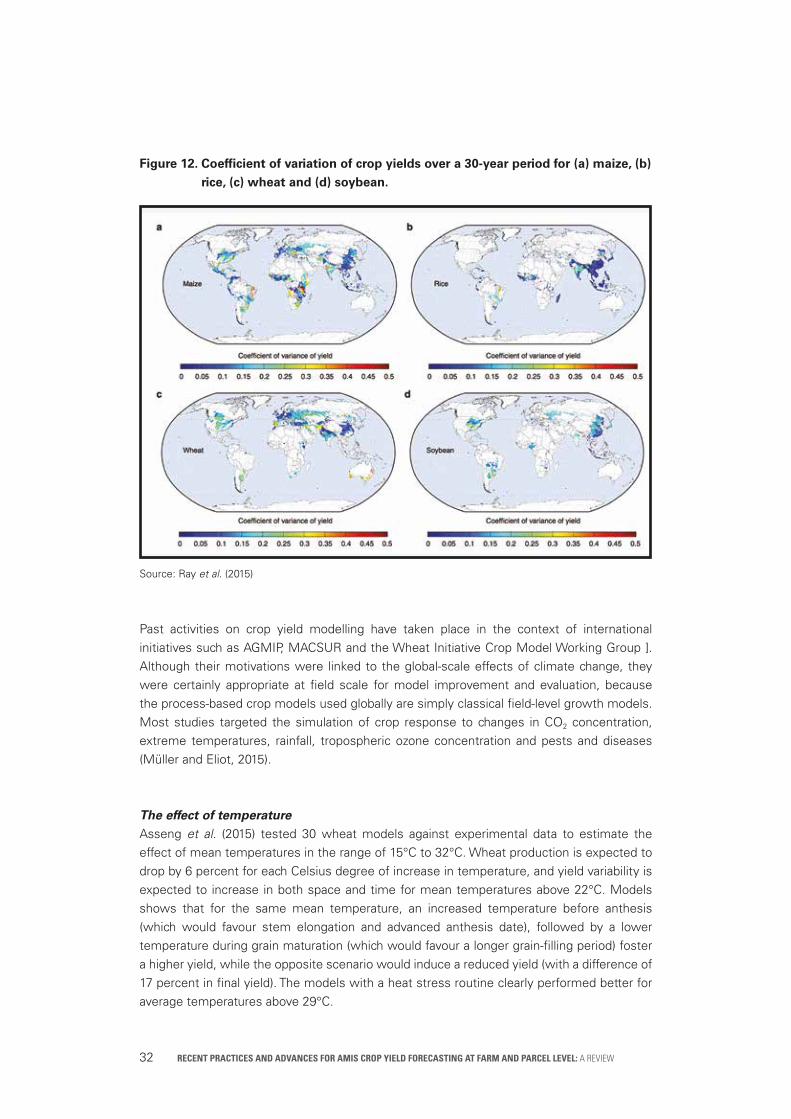
Recently, Ray et al. (2015) considered the influence of inter-annual climate variations on crop yields in different regions. On average, 30 percent of the variability experienced in the last 30 years may be explained by variations in temperature and/or rainfall; however, in the less productive zones, this percentage may reach 60 percent. Among the crops of wheat, rice, maize and soybean, rice is the least weather-dependent. Only 53 percent of rice areas showed a significant correlation, with a year-to-year yield variability of 0.1tonne/ha; precipitation variability is more explanatory of the variability in South Asia, and temperature variability of that in Southeast and East Asia. To the contrary, maize showed a significant correlation on 70 percent of the planted areas, for a variability of 0.8 tonnes/ha, 41 percent of which may be explained by the climatic conditions. Temperatures explained the yield in cold countries (Canada) as well as in warmer ones (Spain).

6


Figure 12. Coefficient of variation of crop yields over a 30-year period for (a) maize, (b) rice, (c) wheat and (d) soybean.

Source: Ray et al. (2015)

Past activities on crop yield modelling have taken place in the context of international initiatives such as AGMIP, MACSUR and the Wheat Initiative Crop Model Working Group ]. Although their motivations were linked to the global-scale effects of climate change, they were certainly appropriate at field scale for model improvement and evaluation, because the process-based crop models used globally are simply classical field-level growth models. Most studies targeted the simulation of crop response to changes in CO2 concentration, extreme temperatures, rainfall, tropospheric ozone concentration and pests and diseases (Müller and Eliot, 2015).

The effect of temperatureAsseng et al. (2015) tested 30 wheat models against experimental data to estimate the effect of mean temperatures in the range of 15°C to 32°C. Wheat production is expected to drop by 6 percent for each Celsius degree of increase in temperature, and yield variability is expected to increase in both space and time for mean temperatures above 22°C. Models shows that for the same mean temperature, an increased temperature before anthesis (which would favour stem elongation and advanced anthesis date), followed by a lower temperature during grain maturation (which would favour a longer grain-filling period) foster a higher yield, while the opposite scenario would induce a reduced yield (with a difference of 17 percent in final yield). The models with a heat stress routine clearly performed better for average temperatures above 29°C.


Frost damage is a well-known limiting factor in the Northern hemisphere. Recently, however, the heat stress undergone by cereals (including rice) during the reproductive period has drawn the attention of researchers, because heat stress accelerates the overall plant senescence and grain-filling process, thus resulting in an earlier maturity date and a shorter reproductive period. Due to the poor performance of major models such as APSIM or CERES, several routines (all heat-stress-related) have been developed for rice, wheat, soybean, sunflower and peanuts. Liu et al. (2016) looked at the post-heading duration due to heat stress for wheat in 160 agrometeorological experimental stations in China from 1981 to 2010. The performances of four widely used temperature response routines from four wheat models (APSIM-Wheat’s Bilinear routine; CERES-Wheat’s Trapezoidal routine; GECROS’s Beta routine; and WheatGrow’s Sin routine) were evaluated using the WheatGrow model. Because all routines failed to predict the reduction in duration, the first three models were successfully modified by including an additional heat thermal effect (HTE) quantified with heat degree days (HDD) and GDDs in the thermal effect on wheat development. All routines with the HTE function predicted shorter post-heading duration under heat stress, which agreed with the observations, and remarkable improvements in simulation accuracy were observed (RMSE = 2.3 days).

Limiting their study to maize, Bassu et al. (2014) used a set of 23 models to study yield variation due to increased temperature and CO2 concentration in Brazil, France, the United Republic of Tanzania and the United States of America. Forecasted yield decreased by 0.5 Tonnes/ha per Celsius degree increase and was boosted by 7.5 percent on average when CO2 concentration was shifted from 360 to 720 μmol mol-1 CO2.

The effect of rainfallAsseng et al. (2016) have screened the use of accurate 10-day advanced rainfall forecasts for anticipating rain-fed wheat sowing dates, and management decisions on late nitrogen fertilization and fungicide spraying in Australia. Interestingly, the potential gains are converted in A$/ha, corresponding to the recent trend of using crop simulation models to improve farm management, by providing farmers with a range of decision management options (for an average farm size of 2 000 ha). The APSIM model was applied on a 25-year historical time series. Depending on soil type and rainfall at each specific location, the gross margin obtained from dry-sowing varied between A$/ha 10 and 100 per ha, reaching A$/ha 160 ha when associated with late nitrogen and anti-rust fungicide applications.

The effect of CO2 concentrationIn the context of climate change, the initial statement that increased CO2 concentration had a positive effect on crop yields was subsequently challenged. O’Leary et al. (2015) base their analysis of wheat biomass at anthesis and final yield on the modifications of the RUE and TE for six crop growth simulation models (including APSIM, SALUS and CROPSYST). Although not all models adequately reproduce the initial growth, all models correctly reflected the experiment’s final results. At the increased concentration (550 versus 365 μmol mol-1 CO2), the final yields were increased by 21 to 23 percent (in both dry and wet conditions) and water use reduced by 20 mm, leading to a 30 percent increase in water use. The simultaneous


increase of temperature of 1°C reduced the yield increase to some extent, probably due to a reduction of the period for grain filling.

Li et al. (2016) examined the rice yield under increased CO2 concentration and air temperature. Compared to observation data, models generally tended to overestimate the positive effects of CO2 concentration and underestimate the negative effects of increased temperature.

The effect of ozone (O3)Although ozone is considered to affect stomatal conductance, photosynthesis efficiency, leaf ageing and yield, limited work has been done to add an O3 module to crop growth models. Recently, WOFOST (Capelli et al., 2016) was adapted and tested for wheat (high sensitivity) and barley (low sensitivity) in Germany and Spain. For O3 concentrations ranging from 20 to 60 ppb, effects on wheat yields reaching 30 percent were found in conditions not constrained by water stress, and of 10 percent for water-limited (rain-fed) conditions. In addition, Ghude et al. (2014) examined O3 influence on cotton, soybean, rice and wheat crops in India. Using the AOT40 metrics proposed by Hollaway et al. (2012), they estimate the expected cereals production reduction in India at 9.2 percent.

IntercroppingCarlson et al. (2016) incorporated maize and bean intercropping in the CROPSYST model considering the light interception shares among the two crops, as well as their water and nitrogen intakes in non-limited and limited conditions. The simulation results compared to observations for 2015 in Kenya show a good fit for green area index and biomass for both crops, confirming the advantage of intercropping for yield maximization. The STICS model was also adapted to enable simulations in cases of arable intercropping. Bocar Baldé (2016) illustrates its application to the maize and pigeon-pea crops in Brazil and millet and cowpea crops in Senegal.

The effect of pests and diseasesIt is currently estimated that the effect of pests and diseases reduces actual global food production by 16 percent, such that modelling such factors in agricultural crop systems is one of the current priorities. Readers interested in the state of the art on merging pest and disease models with crop models should refer to the proceedings of the 2015 workshop on “Advancing Pest and Disease Modeling” held by the University of Florida in Gainesville, Florida, United States of America from 23 to 25 February 20151. Boote et al. (2015) summarize the models involved (DSSAT, CROPGRO and CERES), the crop concerned (maize, soybean, millet and peanut) and the parameters modelled.

The current situation is that all models require the entry of pest damage (as scouting data) to enable ex post facto evaluation of yield losses to pests in research experiments. In the

1 http://conference.ifas.ufl.edu/pest/index.html.


future, the objective should be to create simple simulators of disease damage as a function of temperature, humidity, rainfall, crop stage, genetics and fungicide efficacy. Coupled with the crop model, this would enable predicting the effects of disease on crop yields without the need to input disease damage.

Bregaglio et al. (2015) retained an alternative approach, favouring the development of modular routines that are sufficiently generic to cover various pathogens and crops that could be integrated in more than one crop growth model. The four software components proposed cover the production of primary inoculum and the occurrence of primary infections (InoculumPressure), the development of secondary infection cycles during the cropping season (DiseaseProgress), the interactions between epidemic development and crop physiological processes (ImpactsOnPlants) and the impact of agricultural management practices on disease development (Agro-managementDisease), quantifying the disease effect on LAI reduction and RUE reduction (CERES, CROPSYST, STICS, WARM, DSSAT, APSIM) or alternatively CO2 assimilation (SUCROS, WOFOST, ORYZA). Willocquet et al. (2008) provide details on the modelling of LAI and RUE reductions in WHEATPEST and RICEPEST. The results of the simulations were successfully compared to field measurements for rice blast and wheat brown rust in China and Europe using the WOFOST and WARM models.

AGMIP has recently launched its Pests and Diseases Model Intercomparison Project, the first workshop regarding which took place in Toulouse, France in October 2016. During said workshop, it was resolved to set up an ad hoc working group.

Analysis of the yield gapThe compilation of the Global Yield Gap Atlas (or GYGA; see www.yieldgap.org) provided an opportunity to express recommendations to enhance the comparability of the outputs of crop models. As shown in Figure 13, the process consists in aggregating local crop growth model runs up to the regional or national level.

Figure 13. Global yield gap protocol for data aggregation.

Source: van Bussel, L.G.J. (2015).


As illustrated by Gobbet et al. (2016) when estimating wheat exploitable yield for wheat in Australia (with additional exports estimated at US$ 3.2 billion), the GYGA protocol recommends paying attention to the quality of input data (crop mask, climatic zones based on annual GDDs, temperature seasonality and an aridity index, weather stations 200 km apart in operation for 15 to 20 years, unbiased soil sample location) and the local suitability of the selected crop model to forecast the water-limited yield. The same method was applied for rice (van Oort et al. 2015) on eight African countries (Burkina Faso, Egypt, Ghana, Mali, Nigeria, United Republic of Tanzania, Uganda and Zambia) to estimate their yield gap using ORYZA2000 (which was adapted to correctly estimate heat-induced sterility in semi-arid zones) and concluded that the actual rice areas could not lead to national self-sufficiency. In the same way, with the DSSAT model, van Bussel et al. (2015) estimated the yield gaps for soybean (32 percent), maize (41 percent) and wheat (41 percent) in Argentina. The countries currently included in the atlas account for 60, 58, and 35 percent respectively of the global rice, maize and wheat production. In addition to grains (maize, rice, wheat, sorghum and millet), soybean, potato and sugarcane have been added, reaching coverage of 43 countries.


Role of the private sector: insurances, start-ups, industry and foundations

In recent years, the interest of the private sector for crop yield modelling has been growing. Bearing smallholder farmers in mind, the Bill & Melinda Gates Foundation has financed several projects relating to this theme (e.g. STARS, NEXTGEN and GEOSHARE). The major actors are very close to the leaders of the AGMIP and the main outcome has been a special 2016 issue of the Agricultural Systems academic journal, entitled “Next-generation agricultural system data, models and knowledge products”. Various papers recommend how such modelling should evolve, concentrating efforts on data quality and free access, software modularity, the gaps (pest and disease damage evaluation) and the need for simple mobile apps for extension advisors and large farms. The process also envisages integration of a socioeconomic module.

The food industry has structured its cooperation by establishing initiatives such as the international Life Sciences Institute (ILSI) and CIMSANS, building and sharing joint databases such as the AgTrials database, maintained by the Centro Internacional de Agricultura Tropical (CIAT), and the World Food Life Cycle Assessment database (WFLCAB). The food industry’s interest in understanding the preferences of future customers – which enables industry operators to adapt their offer and plan what, where and how to produce – prompts its exploitation of the farmer data that may be gleaned from contractual agreements relating to the certification and purchase of raw products. Its strategy consists in establishing connections with the academic sector to identify the operational models that could be incorporated in their usually basic models. Agro-chemical companies from the United States of America and the European Union have also identified crop yield modelling as one of the components of the precision farming that they wish to offer to foster their business expansion. Their strategy

7


has usually been to buy over start-up companies, which enables them to gain time in terms of industry innovations.

Crop insurance companies are active in crop yield modelling during risk evaluation (premium calculation) and during claims liquidation. In 2011, the worldwide agricultural insurance premium reached US$ 23.5 billion. North America held 55 percent of the market share, Europe 18 percent, Asia 22 percent, Oceania 0.8 percent and Africa 0.5 percent. In Asia, China held 45 percent of the market. To clarify why a priori risk evaluations are necessary, suffice it to mention that the 2012 drought in the United States of America cost the crop insurance program over US$ 17 billion; and that in China, the 2013 premiums and claims arising from the country’s crop insurance program amounted to CNY 31 and CNY 22 billion respectively.

Insurers and reinsurers must therefore calibrate their contractual terms with historical data, modelling technological trends as well as climatic effects (including extreme events), and merge these with the price models driving the current year’s crop hectares and management practices. As an example, the AIR Worldwide suite of software (Vergara et al., 2014), adopted by Munich Re in 2013, will be examined. AIR Worldwide monitors crops such as corn, rice, wheat, soybean and cotton for damages due to frost, wind, drought and flood. The AIR approach consists in modelling the effects of climate through a crop computed through an Agricultural Weather Index (AWI) specifically per country, on the basis of daily temperatures (minimum and maximum, on a 50-km grid) and precipitations (on a 25-km grid). The main indicators derived are the GDDs and evapotranspiration. In addition, soil information allows adding outputs on runoff, soil moisture and plant available water capacity. The historical data consist of observed county yield, planting dates and phenological stages. Historical and current wind records are also used. Although no detail is shared on the exact model equation(s), Zuba et al. (2005) describe it as follows: “[c]ompared to other crop growth models, the underlying methodology for the AWI favors simpler parameterization of yield-related crop growth and crop damage. Calibration of the model is done by adjusting a small number (3 to 4) coefficients used to optimally scale the effect of different weather perils on crop stand.” Therefore, it may be concluded that although no part of the classical complex crop growth model is adopted, with the exception of radiation efficiency and energy repartition, the major processes driving the biomass formation are included.

At the level of evaluating insurance losses, the first aspect to examine is the type of contract. In many developing countries, the work required to evaluate damages has been avoided by favouring index-based insurances (Gommes et al., 2013), in which farmers’ indemnities are based only on trigger points of meteorological observations, such as precipitations or minimum/maximum temperatures. If the contract covers revenues instead of production, the maximum commodity price between harvest time and contract signature date is generally incorporated in the damages evaluation. If the claims are based on individual production losses, the fieldwork associated with the damage quantification (yield/area) may be very costly compared to the amounts claimed, and alternative model-based methods have been identified (de Leeuw et al., 2014). If official crop insurance systems have adopted technology, the private sector has been reluctant and few references are available. Hongo et al. (2015) report that due to low temperatures in 2003, 2.92 million Japanese farmers declared damages


to their insurance companies, which required 173 000 days of work from 84 000 assessors for an overall assessment cost of US$ 10 million. Working on rice, the authors adjust a regression model that links yield and spectral reflectance (NDVI and individual channels of SPOT and ALOS) to obtain RMSEs of 500kg/ha. Taking the example from 2003, they consider that the assessment cost could have been reduced by a factor of 20 if an approach based on remote sensing had been used.

The breeding sector has also begun to study crop growth models, seeking to extract from large-scale breeding trials the genetic parameters required to calibrate crop growth models. Hwang et al. (2015), Technow et al. (2015) and Lamsal (2016) provide an overview of the models’ integration and related problems. The traditional approach consists in fitting a statistical model for genotype-specific parameters (GSPs) versus genotype codes (+1/-1 values), assuming that the crop simulation model is satisfactory. A more recent approach considers that gene markers enable definition of Quantitative Trail Loci (QTLs). These main factors and their interaction with the environment (which is weather-, site- and year-specific) allow for the estimation of CSM parameters through general mixed linear models. Among the models already studied, examples drawn from the DSSAT are presented for soyabean (CROPGRO), wheat and maize (CERES).

Farm decision systems have been the priority of many start-up companies and universities. Capalbo et al. (2016) provide an example of the data, models and knowledge products that are being developed to respond to the needs of farms and information to support policy decisions. They describe general features of these systems and the benefits they could provide to producers as well as research and policymaking. The authors present two models that could be used in farm decision systems: (1) a farm-level decision model and (2) a regional policy analysis tool. An application of these models to the adaptation of wheat systems in the Pacific Northwest region of the United States of America is used to illustrate the models and the way they could be linked to “big data” infrastructure. At farm level, they present the AgBiz logic software created by Oregon State University. Capable of coping with net revenue maximization and alternative management scenarios, the system relies on modules dedicated to climate indicators and metrics, financial aspects, environmental outputs. Unfortunately, no detail is given on the yield models retained. AgroClimate, another decision system, was developed by the University of Florida (Fraisse et al. 2006). Using DSSAT-CSM as a crop model, they monitor 16 crops to understand the influence of an excess or shortfall of water, and the effect of frost and diseases. The forecasts are improved by incorporating those made by the El Niño Southern Oscillation Multivariate Index (ENSO-MEI). The application is well documented in a workbook (http://agroclimate.org/workbook/AgroClimateWorkbook-Print.pdf). Yield Prophet is a farm decision tool that was developed in collaboration with the Commonwealth Scientific and Industrial Research Organisation (CSIRO), using the APSIM model for wheat, barley, canola, sorghum and oats. In addition to yield outcome, it provides the expected maturity date and the actual water and nitrogen available to the plant; the software can be accessed on iPads or iPhones in the field, as well as integrated with existing farm technology.

Monsanto’s Climate Field View platform may be considered to exemplify the type of product currently proposed by start-up companies to farmers in the United States of America. Recently


opened to external developers, it is used freely over 50 million ha in the United States of America and is expected to reach usage by paid premium service of over 200 million ha by 2025. It relies on empirical models that are overfed with farmer information and planters and that combine equipment real-time data. Using extremely high-quality data in inputs, the yield forecasts obtained are of equally good value. Therefore, the general sentiment is that start-ups do not adopt the major crop models. As a final example, the Farmer Business Network (Meisner, 2017) issues US yield forecasts in advance to the (USDA) using the real-time information transmitted by the machinery processing the vast territory under their precision-farming-contract management; however, the crop yield models are regression equations that link historical yields, real-time field level information and current-year climatic conditions.


Current recommendationsAs noted by Holzworth (2014, 2015), in recent years, crop simulation models have evolved into agro-system simulation models. The changes initiated with the evolution of user needs, which shifted from pure scientific research to more technical goals linked to food security (yield gap analysis), climate change and policymaking regarding food, feed and bioenergy production. In general, most models began to include more crops and to interlink crop, pasture and livestock modelling. Software modularity favoured the reuse of routines by others and simplified the improvement of the modelled processes. Platforms were created, usually offering a user-friendly interface, which facilitated module selection and authorizing simulations of changes in management practices for assessing resource use and efficiency. Cloud computing and open-source protocols (for non-commercial applications) solve the major problems associated with the access to software and hardware. As a result, models such as APSIM are currently downloaded 100 times a month, and generate approximately 50 scientific papers with up to 1 000 citations yearly.

While more than 250 crop simulation models are currently available, the inclusion of certain topics remains at an embryonic stage. The inclusion of biotic factors in the model is still restricted to a minority of models the purpose of which is to evaluate yield reduction due to weeds, pests and diseases or yield increases induced by intercropping. The incorporation of the gene, environment and management (GxExM) variables has been boosted especially by the breeding industry; models usually produce the classical phenology and biomass outputs, but also information on economic return. Educated farmers and advisors now have access to downscaled models that can run on tablets. APSIM alone has led to the development of tools such as Yield Prophet, WhopperCropper and APSFarm. At the other extreme of the chain, international initiatives such as GEOGLAM (Leo et al., 2016) succeeded in federating most of the teams dedicated to early warning systems, giving real-time access to production forecasts as well as methodological support to those national teams willing to step into the process. It is important to realize that crop yields models are applied at very different scales, ranging from the field to the continent; however, the models involved have always started

8


development at the field level and resist upscaling generally by subdividing the larger region into subsets that are supposed to be homogeneous in terms of the relevant environmental and management variables.

Antle et al. (2015) present their views on the model design to be derived from selected user cases and the experience of the AGMIP project. Their vision proceeds with a shift from the research context to (commercial) decision-making tools, from pure biophysical modelling to a more economic analysis, from main-effect models to models incorporating interactions between the effects of CO2, O3, nitrogen and water, from a simple point model to the parallel run of a set of gridded point-based models, and from a single forecast to sensitivity and model uncertainty analysis.

As occurred in 2003 with the special issue of the European Journal of Agronomy devoted to “Modelling Cropping Systems: science, software and application”, and in 2015 with the special issue of the Agricultural System special issue on “Towards a New Generation of Agricultural System Models, Data, and Knowledge Products”, which assessed the progress made over the last ten years on crop yield modelling and advocated for a recommended path of development, it may be expected that a new generation of modellers will issue a review issue in 2025 to detail that the current projects have evolved into reality and that further new goals may be proposed.


ReferencesAntle, J.M., Jones, J.W. & Rosenzweig, C. 2015. Towards a New Generation of Agricultur-al System Models, Data, and Knowledge Products: Introduction. AgMIP Publication: New York, USA. Available at: http://goo.gl/MjNjHy. Accessed on 18 November 2016.

Antle, J.M., Basso, B.O., Conant, R.T., Godfray, C., Jones, J.W., Herrero, M., Howitt, R.E., Keating, B.A., Munoz-Carpena, R., Rosenzweig, C., Tittonell, P. & Wheeler, T.R. 2015. Towards a New Generation of Agricultural System Models, Data, and Knowledge Products: Model Design, Improvement and Implementation. AgMIP Publication: New York, USA. Available at: http://goo.gl/S9gpUH. Accessed on 18 November 2016.

Agricultural Market Information Systems (AMIS). 2016. Crop Yield Forecasting: Method-ological and Institutional Aspects. FAO Publication: Rome.

Asseng S., Ewert F., Martre P., Rötter R.P., Lobell D.B. et al. 2015. Rising temperatures reduce global wheat production. Nature Climate Change, 5: 143–147.

Asseng S., McIntosh P.C., Thomas G., Ebert E. & Khimashia N. 2016. Is a 10-days rainfall forecast of value in dry-land wheat cropping? Agricultural and forest methodology, 216: 170–176.

Acharya, T., Fanzo, J., Gustafson, D., Ingram, J. & Schneeman, B. 2014. Assessing Sus-tainable Nutrition Security: The Role of Food Systems. Publication of the ILSI Research Foundation, Center for Integrated Modeling of Sustainable Agriculture and Nutrition Se-curity: Washington, D.C. Available at:http://ilsi.org/publication/assessing-sustainable-nutri-tion-security-the-role-of-food-systems/. Accessed on 18 April 2017.

Atzberger C. 2013. Advances in Remote Sensing of Agriculture: Context Description, Ex-isting Operational Monitoring Systems and Major Information Needs. Remote Sensing, 5: 949–981.

Basso B., Cammarano D. & Carfagna, E. 2013. Review of Crop Yield Forecasting Meth-ods and Early Warning Systems. Paper presented at Global Strategy Meeting, Scientific Advisory Committee, 18–19 July 2013. Rome. Available at: http://www.fao.org/fileadmin/templates/ess/documents/meetings_and_workshops/GS_SAC_2013/Improving_methods_for_crops_estimates/Crop_Yield_Forecasting_Methods_and_Early_Warning_Systems_Lit_review.pdf. Accessed on 18 April 2017.

Basso B., Schulthess U. & Carfagna, E. 2014. A comprehensive evaluation of method-ological and operational solutions to improve crop yield forecasting. FAO contract report, unpublished.


Bassu, S., Brisson, N., Drand, J.L., Boote, B., Lizaso, J. et al. 2014. How do various maize crop models vary in their responses to climate change factors. Global Change Biolo-gy, 20: 2301–2320.

Bocar Baldé, A., Laure Tall, L., Bakhoum, N., Affholder, F., Clermont Dauphin, C. et al. 2016. Modeling intercropping with cereals in smallholder agrosystems: from lessons learned in Central Brazil to their application in the Peanut Basin in Senegal. Paper presented at the AgMIP6 Global Workshop, Montpellier, France. 28–30 June 2016. Available at: http://www.agmip.org/wp-content/uploads/2016/07/AlphaBocarBaldeLaureTall_AgMIP_Presenta-tion.pdf. Accessed 18 April 2017.

Bregaglio, S. & Donatelli, M. 2015. A set of software components for the simulation of plant airborne diseases. Environmental Modelling & Software 72: 426–444.

Capalbo, S.M., Antle, J.M. & Seavert, C. 2016. Next generation data systems and knowledge products to support agricultural producers and science-based policy decision making. Agricultural Systems. Available at: http://ac.els-cdn.com/S0308521X16306898/1-s2.0-S0308521X16306898-main.pdf?_tid=82657a20-210a-11e7-b286-00000aacb362&acd-nat=1492171648_497a0f39aca2ac6327a47d9dace26c6e. Accessed 18 April 2017.

Cappelli, G., Stella, T., Confalonieri, R., Van den Berg, M. & Dentener, F. 2016. Simulation of the impacts of tropospheric ozone concentration on plant production. Paper presented at AgMIP Global Workshop, Ozone side session, Montpellier, France. 28–30 June 2016. Avail-able at: http://www.agmip.org/wp-content/uploads/2016/10/Cappelli_Ozone.pdf. Accessed on 18 April 2017.

Carlson, B., Sommer, R., Paul, B., Muli, M. & Stöckle, C. 2016. Enhancing CropSyst for intercropping modeling. Paper presented at iCropM, Berlin. 15–17 March 2016. CIAT Publi-cation: Cali, Colombia.

Chipanshi, A., Zhang, Y., Kouadio, L., Newlands, N., Davidson, A. et al. 2015. Evaluation of the integrated Canadian crop yield Forecaster (ICCYF) model for in-season prediction of crop yield across the Canadian agricultural landscape. Agricultural and Forest Meteorology, 206: 137–150.

Choudhury, I., Chakraborty, M. & Parihar, J.S. 2007. Estimation of rice growth parameter and crop phenology with conjunctive use of Radarsat and Envisat. Proceedings of Envisat Symposium 2007, 23–27 April 2007. Montreux, Switzerland.

Colaizzi, D., O’Shaughnessy, A.S., Evett, S.R. & Howell, T.A. 2012. Using plant canopy temperature to improve crop irrigation management. Proceedings of the 24th Annual Central Plains Irrigation Conference, Colby, Kansas, USA. 21–22 February 2012.

Congalton, R.G., Gu, J., Yadav, K., Thenkabail, P. & Ozdogan, M. 2014. Global Land Cover Mapping: A Review and Uncertainty Analysis. Remote Sensing, 6(12): 12070–12093.


De Leeuw, J., Vrieling, A., Shee, A., Atzberger, C., Hadgu, K.M. et al. 2014. The Potential and Uptake of Remote Sensing in Insurance: A Review. Remote Sensing, 6: 10888–10912.

Di Paola, A., Valentini, R. & Santini, M. 2016. An Overview of available crop growth and yield models for studies and assessment in agriculture. Journal of the Science of Food and Agriculture, 96: 709–714.

Donatelli M., Magarey, R.D., Bregaglio, S., Willocquet, L., Whish, J.P.M. & Savary, S. 2016. Modelling the impacts of pests and diseases on agricultural systems. Agricultural Systems, in press.

Durgun, Y.O., Gobin, A., Gilliams, S., Duveiller, G. & Tychon, B. 2016. Testing the Contribu-tion of Stress Factors to Improve Wheat and Maize Yield Estimations Derived from Remote-ly-Sensed Dry Matter Productivity. Remote Sensing, 8: 170.

Elliott, J. & Müller, C. 2015. The AgMIP GRIDded Crop Modeling Initiative (AgGRID) and the Global Gridded Crop Model Intercomparison (GGCMI). In Hillel, D. & Rosenzweig, C., Handbook of Climate Change and Agroecosystems, Joint Publication with American Society of Agronomy, Crop Science Society of America and Soil Science Society of America (pp. 175–189).

Elliott, J., Müller, C., Deryng, D. et al. 2015. The Global Gridded Crop Model Intercompari-son: data and modeling protocols for Phase 1. Geoscientific Model Development, 8: 261–277.

El Sharif, H., Wang, J. & Georgakakos, A.P. 2015. Modeling Regional Crop Yield and Irri-gation Demand Using SMAP Type of Soil Moisture Data. Journal of Hydrometeorology 16: 904–916.

Eerens, H., Piccard, I., Royer, A., & Orlandi, S. 2004. Methodology of the MARS Crop Yield Forecasting System. Vol. 3: Remote Sensing Information, Data Processing and Analysis. Pub-lication of the Joint Research Centre of the European Commission: Ispra, Italy.

Fraisse, C.W., Breuer, N.E., Zierden, D., Bellow, J.G., Paz, J. et al. 2006. AgClimate: A climate forecast information system for agricultural risk management in the southeastern USA. Computers and Electronics in Agriculture, 53:13–27.

Franch, B., Vermote, E.F., Becker-Reshef, I., Claverie, M., Huang, J., Zhang, J., Justice, C. & Sobrino, J.A. 2015. Improving the timeliness of winter wheat production forecast in the United States of America, Ukraine and China using MODIS data and NCAR Growing Degree Day information. Remote Sensing of Environment, 161: 131–148.

Gommes, R. & Kayitakire, F. 2013. The challenges of index-based insurance for food secu-rity in developing countries. Proceedings of a technical workshop organized by the EC Joint Research Centre (JRC) and the International Research Institute for Climate and Society (IRI), Ispra, Italy. 2–3 May 2012.


Grassini, P., van Bussel, L., Van Wart, J., Wolf, J., Claessens, L. et al. 2015. How good is good enough? Data requirements for reliable crop yield simulations and yield-gap analysis. Field Crops Research, 177: 49–63.

Guerschman, J.P., Scarth, P.F., McVicar, T.R., Renzullo, L.J., Malthus, T.J. et al. 2015. As-sessing the effects of site heterogeneity and soil properties when unmixing photosynthetic vegetation, non-photosynthetic vegetation and bare soil fractions from Landsat and MODIS data. Remote Sensing of Environment, 161: 12–26.

Guerschman, J.P., McKenzie, N.J., Held, A. & Zurita-Milla, R. 2016. Advances in remote sensing for agricultural development and poverty alleviation. In McKenzie, N.J., Sparrow, A.D. & Guerschman, J.P., The role of remote sensing in agricultural development and pov-erty alleviation – the STARS Landscaping Study. CSIRO Australia Publication (Section 3): Canberra.

Gustafson, D.I., Jones, J.W., Porter, C.H., Hyman, G., Edgerton, M.D. et al. 2014. Cli-mate adaptation imperatives: untapped global maize yields opportunities. International Jour-nal of Agricultural Sustainability, 12(4): 471–486.

Hollaway, M.J., Arnold, S.R., Challinor, A.J. & Emberson, L.D. 2012. Intercontinental trans-boundary contributions to ozone-induced crop yield losses in the Northern Hemi-sphere, Biogeosciences, 9: 271–292.

Holzworth, D.P., Huth, N.I., deVoil, P.G., Zurcher, E.J., Herrmann, N.I. et al. 2014. APSIM - Evolution towards a new generation of agricultural systems simulation. Environmental Modeling & Software, 62: 327–350.

Holzworth, D.P., Snow, V., Janssen, S., Athanasiadis, I.N., Donatelli, M. et al. 2015. Ag-ricultural production systems modeling and software: Current status and future prospects. Environmental Modeling & Software, 72: 276–286.

Hongo, C., Tsuzawa, T., Tokui, K. & Tamura, E. 2015. Development of Damage Assessment Method of Rice Crop for Agricultural Insurance Using Satellite Data. Journal of Agricultural Science, 7: 59–71.

Hunt, L.A. & Boote, K.J. 1998. Data for model operation, calibration and evaluation. In Tsuji, G.Y., Hoogenboom, G. & Thornton, P.K. (eds), Understanding options for agricultural produc-tion (pp. 9–39). Springer Netherlands: Doetinchem, The Netherlands.

Hwang, C., Correll, M.J., Gezan, S.A., Zhang, L., Bhakta, M.S. et al. 2016. Next generation crop models: A modular approach to model early vegetative and reproductive development of the common bean (Phaseolus vulgaris L). Agricultural Systems, in press.


Janssen, S., Porter, C.H., Moore, A.D., Athanasiadis, I.N., Foster, I., Jones, J.W. & Ant-le, J.M. 2015. Towards a New Generation of Agricultural System Models, Data, and Knowl-edge Products: Building an Open Web-Based Approach to Agricultural Data, System Mod-eling and Decision Support. AgMIP Publication: New York, USA. Available at http://www.agmip.org/refbase/uploads/janssen/2015/221_Janssen2015.pdf. Accessed 18 April 2017.

Jones, J.W., Antle, J.M., Basso, B.O., Boote, K.J., Conant, R.T. et al. 2015. Towards a New Generation of Agricultural System Models, Data, and Knowledge Products: State of Agricultural Systems Science. AgMIP Publication : New York, USA. Available at: http://goo.gl/f4eVl4. Accessed 18 April 2017.

Jones, J.W., Antle, J.M., Basso, B., Boote, K.J., Conant, R.T. et al. 2016. Brief history of agricultural systems modeling. Agricultural Systems, in press. Available at: http://www.sci-encedirect.com/science/article/pii/S0308521X16301585. Accessed 17 October 2016.

Kastens, J.H., Kastens, T.L., Kastens, D.L.A., Price, K.P., Martinko, E.A. & Lee, R. 2005. Image masking for crop yield forecasting using AVHRR NDVI time series imagery. Remote Sensing of Environment, 99: 341–356.

Lamsal, A. 2016. Crop model parameter estimation and sensitivity analysis for large scale data using supercomputers. Kansas State University, USA (Ph.D. Thesis).

Leo, O., Baruth, B. & Delincé, J. 2016. The MARS, GLOBCAST and GEOGLAM Crop Yield monitoring and forecasting systems and their potential application in Bangladesh. Proceed-ings of the International Seminar on Approaches and Methodologies for Crop Monitoring and Production Forecasting, Dhaka (forthcoming). 25–26 May 2016.

Li, T., Hasegawa, T., Yin, X., Zhu, X. & Boote, K. 2015. Uncertainties in predicting rice yield by current crop models under a wide range of climatic conditions. Global Change Biology, 21: 1328–1341.

Li, T., Yin, X., Hasegawa, T., Boote, K., Zhu, Y. et al. 2016. Improving rice models for more reliable prediction of responses of rice yield to CO2 and temperature elevation. Paper pre-sented at iCropM, Berlin. 15–17 March 2016. Available at: http://agritrop.cirad.fr/580149/. Accessed on 18 April 2017.

Lobell, D.B., Ortiz-Monasterio, J.I. & Falcon, W.P. 2007. Yield uncertainty at the field scale evaluated with multi-year satellite data. Agricultural Systems, 92: 76–90.

Lobell, D.B., Cassman, K.G. & Field, C.B. 2009. Crop yield gaps: their importance, magni-tudes, and causes. Annual Review of Environment and Resources, 34: 179–204.

Lobell, D.B. 2013. The Use of satellite data for crop yield gap analysis. Field Crops Re-search, 143: 56–64


Lobell, D.B., Thau, D., Seifert, C., Engle, E. & Little, B. 2015. A scalable satellite-based crop yield mapper. Remote Sensing of Environment, 164: 324–333.

Liou, Y.A. & Kar S.K. 2014. Evapotranspiration Estimation with Remote Sensing and Vari-ous Surface Energy Balance Algorithms – A Review. Energies 2014, 7 : 2821–2849.

Liu, B., Liu, L., Asseng, S., Zou, X., Li, J., Cao, W. & Zhu, Y. 2016. Modeling the effects of heat stress on post-heading durations in wheat: A comparison of temperature response routines. Agricultural and Forest Meteorology, 222: 45–58

Liu, M., He, B., Lü, A., Zhou, L. & Wu, J. 2014 Parameters sensitivity analysis for a crop growth model applied to winter wheat in the Huanghuaihai plain in China. Geoscientific Model Development, 7: 3867–3888.

Martre, P., Wallach, D., Asseng, S., Ewert, F., James, W., Jones J.W. et al. 2014. Multi-model ensembles of wheat growth: Many models are better than one. Global Change Biol-ogy: 911–925.

McKenzie, N.J., Sparrow, A.D. & Guerschman, J.P. 2016. The role of remote sensing in agricultural development and poverty alleviation – the STARS Landscaping Study. CSIRO Australia Publication: Canberra. Available at: https://publications.csiro.au/rpr/pub?pid=c-siro:EP166562. Accessed 16 November 2016.

Meisner, M. 2017. Early estimates of US crop areas and production from real time monitor-ing of field machinery. Paper prepared for the 61st World Statistics Congress, Marrakech, Morocco. 16–21 July 2017.

Meroni, M., Fasbender, D., Balaghi, R. et al. 2016. Evaluating NDVI Data Continuity Be-tween SPOT-VEGETATION and PROBA-V Missions for Operational Yield Forecasting in North African Countries. IEEE Transactions on Geoscience and Remote Sensing, 54(2): 795–804.

Messina, C.D., Podlich, D., Dong, Z., Samples, M. & Cooper, M. 2011. Yield–trait perfor-mance landscapes: from theory to application in breeding maize for drought tolerance. Journal of Experimental Botany, 62(3), 855–868.

Mohammed, G.H, Goulas, Y., Magnani, F., Moreno, J., Olejnícková J. et al. 2014. 2012 FLEX/Sentinel-3 Tandem Mission Photosynthesis Study – final report. ESA/ESTEC externally contracted report. P&M Technologies Publication: Sault Sainte Marie, Canada. Available at: http://www.flex-photosyn.ca/Reports/PS-Study_FINAL_REPORT_Full_Report_(Public).pdf. Accessed 14 April 2017.

Morell, F.J., Yang, H.S., Cassman, K.J., Van Wart, J., et al. 2016. Can crop yield simulation models be used to predict local to regional maize yields and total production in the US corn belt. Field crops research, 192: 1–12.


Müller, C. & Elliott, J. 2015. The Global Gridded Crop Models Intercomparison: approach-es, insights and caveats for modeling climate change impacts on agriculture at global scale. In A. Elbelhri (ed), Climate change and food systems: global assessments and implications for food security, trade. FAO Publication: Rome.

Müller, C., Elliott, J., Chryssanthacopoulos, J., Arneth, A., Balkovic, J. et al. 2016. Global Gridded Crop Model evaluation: benchmarking, skills, deficiencies and implications. Paper presented at the 6th AgMIP Global Workshop, Montpellier, France. 28–30 June 2016. Avail-able at: http://www.agmip.org/wp-content/uploads/2016/07/4.-160628_ggcmi_evaluation_agmip_gw6_mueller.pdf. Accessed 14 April 2017.

Myneni, R., Hoffman, S., Knyazikhin, Y., Privette, J., Glassy, J. et al. 2002. Global prod-ucts of vegetation leaf area and fraction absorbed PAR from year one of MODIS data. Re-mote Sensing of Environment, 83: 214–231.

Nelson, G.C., H. Valin, R.D. Sands, P. Havlik, H. Ahammad, D. et al. 2013. Climate change effects on agriculture: Economic responses to biophysical shocks. Proceedings of the Na-tional Academy of Sciences 111(9): 3274–3279.

O’Leary, G.J., Cristy, B., Nuttall, J., Huth, N., Cammarone, D. et al. 2015. Response of wheat growth, grain yield and water use to elevated CO2 under a Free-Air CO2 enrichment (FACE) experiment and modeling in semi-arid environment. Global Change Biology, 21: 2670–2686.

Potgieter, A., Hammer, G., Doherty, A. & de Voil, P. 2005. A simple regional-scale model for forecasting sorghum yield across North-Eastern Australia. Agricultural and Forest Mete-orology, 132: 143–153.

Potgieter, A., Lobell, D., Hammer, G., Jordan, D., Davis, P. & Brider, J. 2016. Yield trends under varying environmental conditions for sorghum and wheat across Australia. Agricul-tural and Forest Meteorology, 228: 276–285.

Rana, S.S. & Rana, R.S. 2014. Advances in crop growth and productivity. Publication of the Department of Agronomy, CSK Himachal Pradesh Krishi Vishvavidyalaya, Palampur, India.

Rembold, F., Atzberger, C., Savin, I. & Rojas, O. 2013. Using Low Resolution Satellite Im-agery for Yield Prediction and Yield Anomaly Detection. Remote Sensing, 5: 1704–1733.

Ray, D.K., Gerber, J.S., MacDonald, G.K. & West, P.C. 2015. Climate variation explains a third of global crop yield variability. Nature Communications, 6: 5989.

Rembold, F., Atzberger, C., Savin, I. & Rojas, O. 2013. Using Low Resolution Satellite Im-agery for Yield Prediction and Yield Anomaly Detection. Remote Sensing, 5: 1704–1733.


Rojas, O. 2007. Operational maize yield model development and validation based on remote sensing and agro-meteorological data in Kenya. International Journal of Remote Sensing, 28 : 3775–3793.

Rojas, O., Rembold, F., Delincé, J. & Léo, O. 2011. Using the NDVI as auxiliary data for rapid quality assessment of rainfall estimates in Africa. International Journal of Remote Sensing, 32(12): 3249–3265.

Rosenzweig, C., Elliott, J., Deryng, D. et al. 2014. Assessing agricultural risks of climate change in the 21st century in a global gridded crop model intercomparison. Proceedings of the National Academy of Sciences of the United States of America, 111: 3268–3273.

Rossini, M., Alonso, L., Cogliati, S., Damm, A., Guanter, L. et al. 2014. Measuring Sun-Induced Chlorophyll Fluorescence: an evaluation and synthesis of existing field data. Paper presented at the 5th International Workshop on Remote Sensing of Vegetation Fluo-rescence, Paris. 22–24 April 2014

Saltelli, A., Chan, K. & Scott, E.M. (eds). 2000. Sensitivity Analysis. John Wiley and Sons: Chichester, U.K.

Technow, F., Messina, C.D., Totir, L.R. & Cooper, M. 2015. Integrating Crop Growth Mod-els with Whole Genome Prediction through Approximate Bayesian Computation. PLoS One, 10(6): e0130855.

Thenkabail. P.S. 2010. Global Croplands and their Importance for Water and Food Security in the Twenty-first Century: Towards an Ever Green Revolution that Combines a Second Green Revolution with a Blue Revolution. Remote Sensing, 2(9): 2305–2312.

Van Bussel, L.G.J., Grassini, P., Van Wart, J., Wolf, J. & Claessens, L. 2015. From field to atlas: Upscaling of location-specific yield gap estimates. Field Crops Research, 177: 98–108.

Van Hoolst, R., Eerens, H., Haesen, H., Royer, A., Bydekerke, L., Rojas, O., Li, Y. & Ra-cionzer, P. 2016. FAO’s AVHRR-based Agricultural Stress Index System (ASIS) for global drought monitoring. International Journal of Remote Sensing, 37(2): 418–439.

Van Ittersum, M.K., Cassman, K.G., Grassini, P., Wolf, J., Tittonell P. & Hochman Z. 2013. Yield gap analysis with local to global relevance – A review. Field Crops Research, 143: 4–17.

Van Oort, P.A.J., Saito, K., Tanaka, A., Amovin-Assagba, E. & Van Bussel, L.G.J. 2015. Assessment of rice self-sufficiency in 2025 in eight African countries. Global Food Security, 5: 39–49.

Vergara, O., Wang, H. & Zuba, G. 2014. Agricultural risk modelling to improve market infor-mation systems in developing countries. Cahiers Agricultures, 23: 310–316.


Verger, A., Baret, F., Weiss, M., Filella, I. & Peñuelas, J. 2015. GEOCLIM: A global clima-tology of LAI FAPAR and FCOVER from VEGETATION observations for 1999–2010. Remote Sensing of Environment, 166: 126.

Wallach, D., Thornburn. P., Asseng. S., Challinor. A.J., Ewert. F., Jones. J.W., Rotter. R. & Ruane, A. 2016. Estimating model prediction error: Should you treat prediction as fixed or random? Environmental Modeling Software, 84: 529–539.

Wang, X., He, X., Williams, J.R., Izaurralde, R.C. & Atwood, J.D. 2005. Sensitivity and un-certainty analyses of crop yields and soil organic carbon simulated with EPIC. Transactions of the American Society of Agricultural Engineers (ASAE), 48(3): 1041–1054.

Willocquet, L., Aubertot, J.N., Lebard, S., Robert, C., Lannou, C. & Savary, S. 2008. Simulating multiple pest damage in varying winter wheat production situations. Field Crops Research, 107: 12–28.

Zuba, G., Vergara, O. & Doggett, T. 2005. Using the AIR Weather Index to Estimate the Contribution of Climate to Corn and Soybean Yields in the United States. Paper presented at the Southern Agricultural Economics Association annual meeting. Available at: http://age-consearch.umn.edu/bitstream/35613/1/sp05zu01.pdf. Accessed 14 April 2017.

CONTACT

Agricultural Market Information System (AMIS)Food and Agriculture Organization of the United Nations (FAO) Viale delle Terme di Caracalla, 00153 Rome, Italy

Recent pRa

ctices an

d a

dva

nces fo

R aM

is cRop yield

foReca

sting

at faRM

an

d pa

Rcel level: a review

I7339EN/1/06.17

ISBN 978-92-5-109779-3

9 7 8 9 2 5 1 0 9 7 7 9 3

This publication was prepared with the financial support of the Bill & Melinda Gates FoundationComments and suggestions are welcome and may be sent to: [email protected]

Recent practices and advances for AMIS crop yield ... · recent practices and advances for amis...

Documents

Transcript of Recent practices and advances for AMIS crop yield ... · recent practices and advances for amis...