SDT 244

RECENT FINDINGS ON INTERGENERATIONAL INCOME AND EDUCATIONAL MOBILITY IN CHILE

Autor: Javier Núñez y Leslie Miranda.

Santiago, Jun. 2007

Serie Documentos de Trabajo

N 244

Recent Findings on Intergenerational Income and Educational Mobility in Chile

Javier Núñez Leslie Mianda

Departamento de Economía

Universidad de Chile

Abstract

This paper provides new evidence on intergenerational mobility in Chile. Income mobility elasticities for Chile are the range of 0.52 to 0.67, which stand as fairly high in comparison with the international evidence. We also find that educational mobility is lower for the younger cohorts, suggesting an increase of intergenerational educational mobility in the last decades. Finally, we find evidence of a higher degree of intergenerational persistence at the two extremes of the income distribution, particularly at the top of the distribution. We suggest this mirrors the unusually high income concentration at the top of the Chilean income distribution. Keywords:

Intergenerational mobility, schooling, mobility patterns. JEL: D3, I2, J6.

1

Recent Findings on Intergenerational Income and Educational

Mobility in Chile1

First draft: December 2006

Second draft: Jun 2007

Javier Núñez Leslie Miranda

Department of Economics Universidad de Chile

Abstract

This paper provides new evidence on intergenerational mobility in Chile. Income mobility elasticities for Chile are the range of 0.52 to 0.67, which stand as fairly high in comparison with the international evidence. We also find that educational mobility is lower for the younger cohorts, suggesting an increase of intergenerational educational mobility in the last decades. Finally, we find evidence of a higher degree of intergenerational persistence at the two extremes of the income distribution, particularly at the top of the distribution. We suggest this mirrors the unusually high income concentration at the top of the Chilean income distribution.

Keywords: Intergenerational mobility, schooling, mobility patterns. JEL codes: D3, I2, J6.

Introduction

Much of the literature on inequality in Chile has focused on the inequality of

outcomes, typically the distribution of income, but little is known about the country’s levels 1 We thank Dante Contreras, Florencia Torche, Claudio Sapelli, Marcela Perticara, Osvaldo Larranaga, David Bravo, Claudia Sanhueza, Cristina Risco and Marcelo Fuenzalida for previous discussions, comments and insights. This research has been funded by the Interamerican Development Bank.

2

of inequality of opportunities and its evolution in recent times. A common approach to

assess a country’s degree of equality of opportunities is the notion of intergenerational

mobility: a higher level of equality of opportunities is expected to decrease the effect of an

individual’s early socioeconomic background on his economic achievement in adulthood,

implying therefore a higher level of intergenerational economic mobility, or alternatively, a

lower level of intergenerational transmission of the relative socioeconomic status from

parents to their offspring.

This paper attempts to present and examine part of the recent research on

intergenerational income mobility in Chile. This paper is mostly descriptive in nature. The

main questions that we address are the following. What is the level of intergenerational

income mobility in Chile? How does it compare with the existing international evidence?

Can anything be suggested about the trend in intergenerational mobility in Chile in the past

decades? Finally, what are some of the salient patterns of the process of intergenerational

mobility in Chile? and how do these patters compare with the international evidence? Since

the research in intergenerational mobility is rather recent in Chile, there is a significant

amount of issues ahead yet to be addressed. This work proposes and discusses some of

them.

The next section motivates the paper by providing evidence on the conceptual and

empirical distinctions between the notions of inequality of income vs. inequality of

opportunities. Section 2 presents the theoretical framework, section 3 describes the

empirical strategy, section 4 describes the dataset we use in this study, and section 5

presents the mail results. Section 6 concludes.

1. Inequality of Outcomes vs. inequality of Opportunities in Chile

There has been a long debate about whether inequality, and the policies designed to

deal with it, must focus on the inequality of outcomes or on the inequality of opportunities.

3

Advocates of the latter stress that inequality of outcomes (typically income) depend not

only on circumstances that are beyond the control of the individual, such as parental

background, but also on aspects that are under his or her control, such as effort, choices and

so on. Moreover, some authors have suggested that from a moral standpoint, public policies

should focus on equalizing opportunities instead of outcomes (incomes). In a seminal

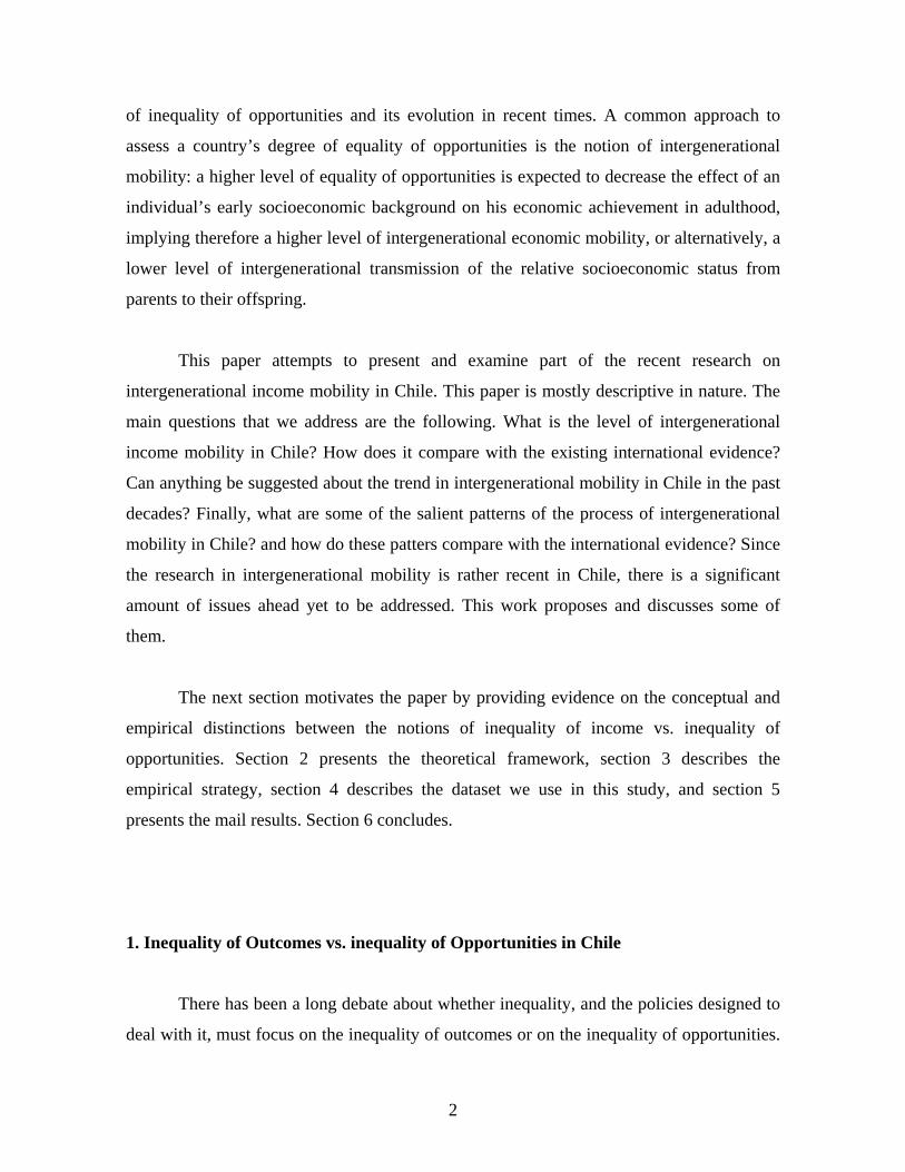
paper, Bourguignon, Ferreira and Melendez (2003) have developed a methodology to

measure the proportion of the income distribution that is explained by inequality of

circumstances of origin such as parental schooling, parents’ occupation and race in Brazil.

The methodology considers not only the direct effect that circumstances have on earnings,

but also the indirect effect of circumstances on earnings through the accumulation of

human capital. They found that the Gini coefficient is reduced in up to 10 percentage

points (about 20 per cent of the Gini) after equalizing the set of circumstances mentioned

earlier.

Table 1: Effect on Gini Coefficient of Equalizing Circumstances in Chile (Greater Santiago)

Núñez and Tartakowsky (2006) apply Bourguignon et. al. (2003) methodology to

Chilean data and they find similar results to their study for Brazil. Table 1 shows the effect

on the Gini coefficient for Greater Santiago of equalizing parental schooling, head of

households age, household size, household composition (single versus biparental), and

parents’ job vulnerability. Even though there can be many relevant unobserved

circumstances, these results do suggest that important circumstances, such as those

mentioned above, play an important yet limited role in shaping income distribution. Hence,

income distribution indicators would only reflect in part a society’s degree and evolution of

equality of opportunities, as they would be affected by other factors. In this context,

Cohort 24-37 38-51 52-65 24-65

Gini Coefficient 0.45 0.51 0.52 0.50

Partial Effect 0.38 0.46 0.43 0.43Total Effect 0.36 0.44 0.4 0.41

Source: Núñez and Tartakowsky (2006)

Gini after Equalizing Circumstances

4

perhaps a closer way of studying equality of opportunities is to examine the

intergenerational income mobility, issue that we address next.

2. Theoretical framework

Following the previous literature, this paper analyzes intergenerational income

transmission using a simplified version of model suggested by Becker and Tomes (1979).

This model assumes that a family only consists of one individual at each generation.

Consider two generations within a given family, father and child. Individual permanent

income Y is assumed to derive from two components: individual endowment of human

capital and individual ability denoted by A. Becker and Tomes assumes that a child’s

endowment of human capital is a result of his father’s optimal allocation of his permanent

income, where the father’s utility depends of his own consumption and the child’s

permanent income. This framework yields the following relationship between father’s and

child’s permanent income: child father childY Y Aφ θ= + (1)

This equation implies that father’s permanent income has a positive causal influence

on child’s earnings or income captured by φ parameter. Equation (1) would also imply a

second source of earnings correlation if child’s ability is correlated to father’s ability.

Parameter θ can be interpreted as a causal effect of previous generations to the next that can

be independent of father’s investment decisions and budget constraints. This parameter will

encompass all aspects of earnings determinants that money cannot buy, such as innate

cognitive abilities, preferences or social networks, among others.

It is important to note that a simple regression of child’s income on father’s income

will capture both transmission mechanisms. Hence, standard OLS estimates of

intergenerational earnings transmission coefficient will provide an upward biased estimate

of the “pure” causal effect of parental income on child’s income. In this paper, we do not

5

separate both effects2. Instead, we are interested in the estimation of reduced-form of

intergenerational earnings regression. It constitutes, however, an important descriptive

measure of the extent of intergenerational earnings mobility.

3. Empirical strategy and data

From the previous framework, if long-rung economic status were directly observed,

the following log-linear relationship between the permanent income of father and child can

be estimated by OLS:

0 1child father

i i iY Yβ β ε= + + (2)

where childiY denotes the log of child’s permanent income in family i and father

iY the log of

his father’s permanent income, and εi is an error term independent of fatheriY usually

assumed to be distributed as N(0,σ2). Our parameter of interest β1 represents the elasticity

of a child’s long-run income with respect to his father’s long-run income. There are two

extreme cases. First if β1=0 there is complete mobility. The income of the child shows no

statistical association with the father’s income. At the other extreme, if β1=1 there is

complete immobility, as a child born from a parent with an income x per cent above the

mean will have an income exactly x per cent above the mean of his own cohort.

However, long-run incomes are not directly observed. Instead, most data sets only

provide measures of current incomes or earnings. Solon (1992) and Zimmerman (1992)

have shown that the use of income in a single year can seriously underestimate the true

intergenerational transmission coefficient due to the presence of transitory components in

current income, especially in combination with the use of a homogeneous sample. A

solution to reduce this bias relies on panel data on fathers’ income to obtain an average of

father’s current income over several years as a proxy for permanent income. Solon (1992)

2 However, see Contreras, Fuenzalida and Núñez (2006) for an attempt to separate both effects using Chilean data.

6

shows that the inconsistency of the transmission coefficient estimator diminishes with the

number of years over which incomes are averaged.

Another problem emerges when, as in this paper, there is no actual income

information of father-child pairs. In this context, a solution proposed by Arellano and

Meghir (1992) and Angrist and Krueger (1992) and followed by Bjorklund and Jantti

(1999) for mobility studies is to use information from two samples: First, earnings

equations can be estimated on an older sample of men in order to obtain coefficients of

some earnings determinants, such as schooling, experience and occupation, for example.

Then, these coefficients can be used to predict the income of the fathers of a sample of

sons, employing the socio-demographic characteristics of the fathers reported by their sons.

This technique is often known as two-sample instrumental variables estimation (TSIV). 3

Assume that the log of father and son’s current income at date t can be written as:

father father father

it i itY Y μ= + (3)

child child childit i itY Y μ= + (4)

where fatheritμ and child

itμ incorporates transitory fluctuations in father and child’s current

income and measurement error. Let fatheriZ denote a set of socio-demographic

characteristics (like age, education, occupation, among others) of fathers from a sample of

families i ∈ I and assume that fatheritY can be written as:

father father father father

it i i itY Z vγ μ= + + (5)

where fatheriv is independent of father

iZ . fatheritY it is not observed in sample I. Yet, if there

exists a sample J from the same population as I, it can be used to provide an estimate of γ,

$γ , derived from estimation of following equation:

3 Although Dunn (2004) refers to this method as “two samples two stage least squares”.

7

father father father fatherjt j j jtY Z vγ μ= + + (6)

for j ∈ J. From an OLS estimation of (6) one can obtain predictions of father’s earnings in

sample I: $father fatherit iY Z γ= . This prediction can in turn be used to estimate β1 since

equations (2), (3), (4) and (6) imply:

$( )0 1child father

it i itY Zβ β γ η= + + (7)

where $( )( )1 1child father father

it i it i iv Zη ε μ β β γ γ= + + + − .

In this paper, the estimates of β1 are based on the estimation of equations (6) and (7)

on separate samples as we describe in the following section. In particular, in a first stage we

estimate a Mincer version of equation (6) that allows for different schooling returns by

educational level4:

20 1 2 1 3 2 4 5( 8) ( 12)father

js js js js js js jsY S d S d S Exper Experγ γ γ γ γ γ ε= + + − + − + + + (8)

where Sjs represents the years of schooling of father in year s, 5 Experjs stands for father’s

potential experience6 and εjs is a random error term. In addition, dummy variables are

defined as:

1

1 80

if Sd

otherwise>⎧

= ⎨⎩

2

1 120

if Sd

otherwise>⎧

= ⎨⎩

In another specification we also use information of fathers’ occupation that comes

from a new survey realized in the middle of year 2006 to a sub-sample of the June 2004

version of Employment and Unemployment Survey of the Universidad de Chile, under the

assumption that occupation is a good instrument to estimate the father’s permanent income.

4 In Chile, elementary education consists of the first eight years and secondary school consists of four additional years. 5 The s year corresponds to time when father were taken investment decisions on his child’s human capital. 6 Potential experience is defined as: age minus years of schooling minus 6.

8

In a second stage, we use the estimated parameters in (8) and fathers’ information

reported by the sons to predict the fathers’ income, as follows:

20 1 2 1 3 2 4 5( 8) ( 12)

fatheris is is is is isY S d S d S Exper Experγ γ γ γ γ γ= + + − + − + + (9)

Hence, we obtain the intergenerational income elasticity β1 from:

20 1 2 3

fatherchildisit it it itY Y age ageβ β β β η= + + + + (10)

where ageit stands for child’s age and controls for life-cycle profiles in child’s earnings.

Data

At the outset it must be stressed that unfortunately Chile does not have a nationally-

representative survey of sons with data including fathers’ characteristics that are likely to

be correlated with long run earnings7. Our dataset comes from the Employment and

Unemployment Survey for the Greater Santiago conducted annually by Universidad de

Chile since 1957 and it is applied to approximately 4,000 households. This is important

because the intergenerational income elasticities are likely to underestimate the nationwide

elasticities, as the result of having a more homogeneous sample and leaving out parts of the

population were intergenerational socioeconomic persistence is expected to be higher, such

as the remote and rural areas as well as small urban areas, as we will discuss later.

In order to avoid selectivity issues associated with female participation in labor

market, we focus only on father-son intergenerational income mobility. The analysis of

intergenerational income mobility involving mothers and daughters remains as future

research. However, we consider sons as well as daughters when we examine

intergenerational educational mobility in section 5.2.

7 The CASEN survey (Encuesta de Caracterización Socioeconómica) may be a possible database with this information but only for a sample of sons that live with their parents. Hence, problems arise from potential selection bias. Currently, we are working with this data and we are trying different solutions to address this problem.

9

The Employment and Unemployment Survey provides information on gender, age,

educational level, employment status, occupational position, economic sectors and monthly

income from wages, salaries and self-employment. All this information is relevant to

estimate coefficients of Mincer equations that are employed to predict the unobserved

income of fathers. Mincer equations like (8) were estimated for the male labor force in 15-

65 age range with positive income and working at least 30 weekly hours.

Our sons’ sample comes from the June 2004 version of the survey. In this year,

additional to demographic and economic data, respondents were required to provide

information about education and individual characteristics of their parents. We consider

sons in the 23-65 age range to control for selectivity problems in samples outside this

range. We eliminate unemployed and inactive individuals, with no positive incomes and

missing parental information. Our sample was composed by 649 father-son pairs in the

relevant age range.

Fathers’ predicted income was estimated dividing the sons’ sample in three sub-

samples by age cohort: 23-34, 35-44, 45-54 and 55-65. We select our fathers’ samples by

assuming that the father’s relevant investment decisions in human capital, which are

expected to be a major source of socioeconomic transmission across generations, were

taken approximately when the child was between 6 and 18 years old. These years

correspond to 1987, 1977, 1967 and 1958 versions of the Employment and Unemployment

Survey for the 23-34, 35-44, 45-54 and 55-65 cohorts, respectively. Those are periods of

relative economic stability; hence, estimated coefficients of Mincer equations for

mentioned years are similar to those of adjacent years.

A second data source comes from a new survey realized in the middle of year 2006

to a sub-sample of males previously surveyed in the Employment and Unemployment

Survey of June 2004. In this new survey, individuals were required to provide additional

information about specific occupation and other individual characteristics of their parents,

as well as diverse family background information corresponding to period when they were

10

about 15 years old. We use additional information about father’s occupation8 to estimate

another specification of Mincer equations under the assumption that occupation is a good

instrument to estimate the father’s permanent income, in addition to fathers’ schooling and

potential experience.

4. Results

4.1 Estimates of intergenerational income mobility for Chile

Table 2 reports intergenerational regression coefficients for labor incomes9. Results

are reported for the full sample in 23-65 age range. Estimates in this table are obtained

using father’s education, potential experience and occupation as predictors for father’s

income. First-step income regressions are provided in Table A.1 and A.2 in the appendix.

Table 2: Estimates of Intergenerational Labor Income Elasticity by TSIV

(Greater Santiago)

Table 2 indicates that fathers’ predicted log income has a significant positive effect

on their sons’ log income. For the whole sample, the estimated elasticity is around 0.52-

0.5410 depending on the predictors employed.

Table 3 reports the results of various recent intergenerational income mobility

studies. Note that many of them employ the Greater Santiago sample, excepting those that

employ the SIALS database (Contreras et. al.) It is interesting to note that employing only

the SIALS data for the Metropolitan Region (slightly larger than Greater Santiago) yield 8 The 5-level occupational categories are: employer (1); self-employed (2); employee (3); blue-collar worker (4) (reference) and domestic (household) workers (5). 9 The estimates using personal incomes yield the same global elasticity. 10 This number is a weighted average of elasticities of each age group.

Cohort Schooling and Experience

Schooling, Experience and Occupation

24-65 0.54 0.52

Father's income predicted from:

11

fairly similar results that the Greater Santiago studies. In this context, the 0.67 elasticity

obtained from the national urban SIALS database seems closer (but perhaps still an

underestimate) of the country’s intergenerational income elasticity. Another piece of

evidence that reinforces this idea is the pattern of income mobility in Brazil, according to

Ferreira and Veloso (2004): The more prosperous and more urban Brazilian Southwest has

lower income elasticity than the rest of the country, and much lower than the poorer

Northeast region.

Table 3: Evidence on Intergenerational Income Mobility for Chile

Table 4 summarizes some selected evidence on intergenerational mobility. As can

be seen, Chile presents relatively low intergenerational income mobility as compared to

other developing and developed countries. Levels of intergenerational mobility in Chile are

somewhat similar to Brazil’s.11 Some authors have suggested and provided some evidence

of an overall positive relationship between cross-sectional income inequality and

intergenerational persistence of inequality. 12 From this perspective, the evidence for Chile

seems consistent with this hypothesis considering that Chile has a particularly unequal

distribution of income.

11 In this context, for comparison purposes it would be useful to obtain intergenerational incomes elasticities for large urban areas in Brazil. 12 See Dunn (2004).

Study Database Father's Income Predictors Population Son's cohort Elasticity

Nuñez and Risco (2004) Employment and Unemployment Survey

Potential experience, schooling

Greater Santiago 23-55 0.55

Nuñez and Risco (2004)

Employment and Unemployment Survey and CASEN (Fathers'

sample)

Potential experience, schooling

Greater Santiago 23-35 0.43

Contreras, Fuenzalida and Núñez (2006) SIALS Schooling Greater

Santiago 23-55 0.58

Contreras, Fuenzalida and Núñez (2006) SIALS Schooling National

Urban 23-55 0.67

This study Employment and Unemployment Survey

Potential experience, schooling

Greater Santiago 23-65 0.54

This study Employment and Unemployment Survey

Potential experience, schooling, occupation

Greater Santiago 23-65 0.52

12

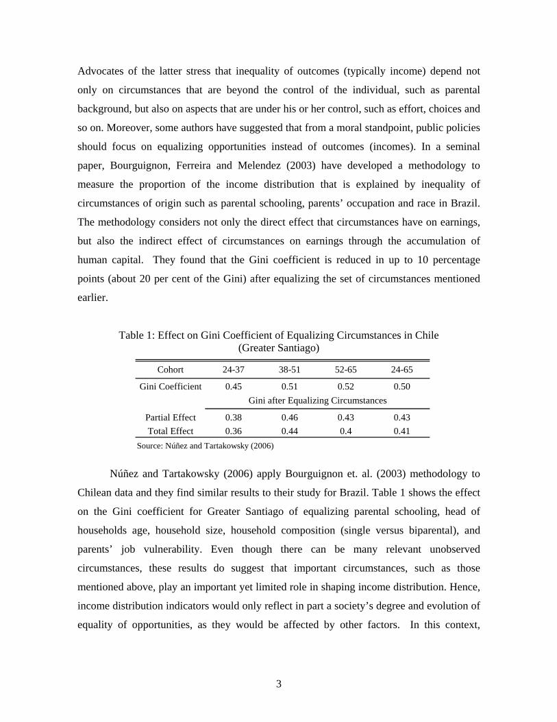
Table 4: International Evidence on Intergenerational Income Mobility

4.2 Evolution of Intergenerational Mobility in Chile

Table 5 presents the intergenerational income elasticities by cohort employing the

fathers’ predicted income from schooling and experience only.

Table 5: Estimates of the Coefficient of Intergenerational Income Mobility

As can be seen, the elasticity coefficient is monotonically decreasing for the three

younger cohorts. A possible explanation of this phenomenon is that intergenerational

mobility could have increased in the last decades. However, this pattern can also be

associated with life-cycle effects on earnings, and therefore whether income mobility has

increased in time is unclear.13 Yet, in order to shed some light on intergenerational mobility

in Chile, in this section we make a detour to examine whether there has been an increase in

13 See Dunn (2004) for a discussion on the role of life-cycle effects on intergenerational income mobility elasticities.

Cohort Personal Income Labor Income23-34 0.46 0.4635-44 0.54 0.5245-54 0.63 0.6555-65 0.59 0.58

All sample 0.54 0.54

Study Country Son's cohort OLS IVOsterbacka (2001) Finland 25-45 0.13Corak and Heisz (1999) Canada 29-32 0.23Lillard and Kilburn (1995) Malaysia >18 0.26Grawe (2001) Malaysia not reported 0.54Björklund and Jänti (1997) Sweden 29-38 0.28Wiegand (1997) Germany 27-33 0.34Lefrane and Trannoy (2004) France 30-40 0.36-0.43Solon (1992) U.S. 25-33 0.29-0.39Solon (1992) U.S. 25-33 0.45-0.53Dearden, Machin and Reed (1997) U.K. 33 0.39-0.59Grawe (2001) Nepal 0.44Grawe (2001) Pakistan 0.46Dunn (2004) Brazil 25-34 0.53 0.69Ferreira and Veloso (2004) Brazil 25-64 0.58Ferreira and Veloso (2004) Brazil (Southeast) 25-64 0.54Ferreira and Veloso (2004) Brazil (Northeast) 25-64 0.73Ferreira and Veloso (2004) Brazil (South) 25-64 0.62Ferreira and Veloso (2004) Brazil (Midwest) 25-64 0.55

Elasticity

13

intergenerational educational mobility. For this purpose, we employ the argument that the

accumulation of schooling for the majority of the population in Chile happens before the

early twenties, such that schooling levels remain fixed throughout the life cycle after the

mid twenties or so. This would imply that life-cycle effects in years of schooling would not

be important for the population in 23-65 age group. Accordingly, the existence of lower

intergenerational mobility coefficients for the younger cohorts would be an indication of a

change in the levels of educational mobility in time.

In order to substantiate this claim we explore the accumulation of schooling in Chile

by age groups using the 1996-2001 CASEN Panel. Figure 1 shows the average individual

accumulation of schooling in Chile by age groups between 1996 and 2001. Figure 1 shows

that while schooling accumulation is significant before 20, it decreases thereafter, and in

fact, it remains negligible after age 25. Hence, we claim that life-cycle effects in years of

schooling are not important for the age group 23-65 considered in this study, and therefore

finding evidence of higher intergenerational educational mobility for the younger cohorts

would be suggestive of increasing educational mobility in time.

Figure 1: 1996-2001 Average Individual Differential in Years of Schooling by Age

Source: Panel CASEN 1996-2001

Table 6 presents the schooling intergenerational elasticities by cohorts. The

evidence indicates lower values for the younger cohorts, although some stability in the last

-1.0

0.0

1.0

2.0

3.0

4.0

5.0

5-9 10-14 15-19 20-24 25-29 30-34 35-39 40-44 45-49 50-54 > 54

Age Cohort

Ave

rage

diff

eren

tial i

n ye

ars o

f sch

oolin

g

14

two cohorts. Using the argument presented above, this would suggest an overall increase in

intergenerational educational mobility in the last decades.

Table 6: Schooling Elasticity by cohort

Tables 7 and 8 provide more evidence of this pattern. While Table 7 reports the

regression results with sons’ schooling as dependent variable, Table 8 reports the

intergenerational schooling elasticity. Tables 7 and 8 provide evidence of a positive

association between fathers’ and sons’ schooling levels, as well as strong evidence of an

expansion in schooling in time, particularly for daughters, as indicated by the coefficients

of year of birth (cohort variable). But Tables 7 and 8 also provide strong evidence of a

significant lower association between fathers and sons’ schooling the younger the cohort, as

indicated by the coefficients of the father’s schooling-cohort interactive term in both

specifications.

Table 7: Cohort Effects in years of schooling.

Dependent Variable: Sons’ Schooling

Cohort Sons and Daughters Sons Daughters

23-34 0.15 0.15 0.14(7.48)** (7.70)** (4.14)**

35-44 0.15 0.15 0.15(6.48)** (4.12)** (5.55)**

45-54 0.29 0.24 0.37(9.75)** (6.59)** (7.57)**

55-65 0.37 0.41 0.32(7.97)** (5.34)** (6.82)**

All sample 0.21 0.21 0.23Robust t statistics in parentheses* significant at 5%; ** significant at 1%

Variables All Sons DaughtersFather's schooling 17.183 14.440 19.945

(5.21)** (3.06)** (4.29)**Father's schooling*Cohort -0.009 -0.007 -0.010

(5.09)** (2.98)** (4.21)**Cohort 0.119 0.022 0.089

(7.10)** (7.00)** (3.55)**Constant -223.716 -40.527 -165.007

(6.83)** (6.65)** (3.36)**Observations 1197 649 548Adj. R-squared 0.33 0.29 0.38Note: Cohort is defined as offspring's year of birth.Robust t statistics in parentheses* significant at 5%; ** significant at 1%

15

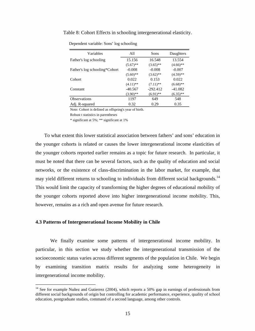
Table 8: Cohort Effects in schooling intergenerational elasticity. Dependent variable: Sons’ log schooling

To what extent this lower statistical association between fathers’ and sons’ education in

the younger cohorts is related or causes the lower intergenerational income elasticities of

the younger cohorts reported earlier remains as a topic for future research. In particular, it

must be noted that there can be several factors, such as the quality of education and social

networks, or the existence of class-discrimination in the labor market, for example, that

may yield different returns to schooling to individuals from different social backgrounds.14

This would limit the capacity of transforming the higher degrees of educational mobility of

the younger cohorts reported above into higher intergenerational income mobility. This,

however, remains as a rich and open avenue for future research.

4.3 Patterns of Intergenerational Income Mobility in Chile

We finally examine some patterns of intergenerational income mobility. In

particular, in this section we study whether the intergenerational transmission of the

socioeconomic status varies across different segments of the population in Chile. We begin

by examining transition matrix results for analyzing some heterogeneity in

intergenerational income mobility.

14 See for example Nuñez and Gutierrez (2004), which reports a 50% gap in earnings of professionals from different social backgrounds of origin but controlling for academic performance, experience, quality of school education, postgraduate studies, command of a second language, among other controls.

Variables All Sons DaughtersFather's log schooling 15.156 16.548 13.554

(5.67)** (3.65)** (4.66)**Father's log schooling*Cohort -0.008 -0.008 -0.007

(5.60)** (3.62)** (4.59)**Cohort 0.022 0.153 0.022

(4.11)** (7.11)** (6.68)**Constant -40.567 -292.412 -41.082

(3.90)** (6.91)** (6.35)**Observations 1197 649 548Adj. R-squared 0.32 0.29 0.35Note: Cohort is defined as offspring's year of birth.Robust t statistics in parentheses* significant at 5%; ** significant at 1%

16

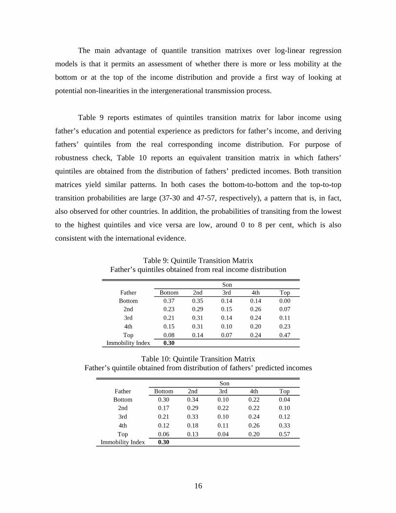
The main advantage of quantile transition matrixes over log-linear regression

models is that it permits an assessment of whether there is more or less mobility at the

bottom or at the top of the income distribution and provide a first way of looking at

potential non-linearities in the intergenerational transmission process.

Table 9 reports estimates of quintiles transition matrix for labor income using

father’s education and potential experience as predictors for father’s income, and deriving

fathers’ quintiles from the real corresponding income distribution. For purpose of

robustness check, Table 10 reports an equivalent transition matrix in which fathers’

quintiles are obtained from the distribution of fathers’ predicted incomes. Both transition

matrices yield similar patterns. In both cases the bottom-to-bottom and the top-to-top

transition probabilities are large (37-30 and 47-57, respectively), a pattern that is, in fact,

also observed for other countries. In addition, the probabilities of transiting from the lowest

to the highest quintiles and vice versa are low, around 0 to 8 per cent, which is also

consistent with the international evidence.

Table 9: Quintile Transition Matrix

Father’s quintiles obtained from real income distribution

Table 10: Quintile Transition Matrix Father’s quintile obtained from distribution of fathers’ predicted incomes

Father Bottom 2nd 3rd 4th TopBottom 0.37 0.35 0.14 0.14 0.00

2nd 0.23 0.29 0.15 0.26 0.073rd 0.21 0.31 0.14 0.24 0.114th 0.15 0.31 0.10 0.20 0.23Top 0.08 0.14 0.07 0.24 0.47

Immobility Index 0.30

Son

Father Bottom 2nd 3rd 4th TopBottom 0.30 0.34 0.10 0.22 0.04

2nd 0.17 0.29 0.22 0.22 0.103rd 0.21 0.33 0.10 0.24 0.124th 0.12 0.18 0.11 0.26 0.33Top 0.06 0.13 0.04 0.20 0.57

Immobility Index 0.30

Son

17

The transition matrixes in Tables 9 and 10 indicate that there is an important

disparity in the intergenerational transmission mechanism. In fact, two salient features can

be pointed out. First, there is more persistence at both extremes of the fathers’ income

distribution, while there is a significant degree of intergenerational mobility in the

intermediate fathers’ quintiles. Second, the matrixes also suggest an asymmetric degree of

intergenerational persistence at the extremes of the fathers’ income distribution, in

particular a higher degree of persistence at the top quintile versus the bottom quintile. In

order to explore these issues further, regression equations of the fathers’ centiles versus

sons’ centiles are reported in Table 11.

Table 11: Alternative Functional Forms for Intergenerational Mobility (Centiles of labor income)

Table 11 shows that the association between the father’s and son’s centile is

increasing as expected but not linearly, in agreement with the evidence reported by the

transition matrixes. In fact, specifications 2 and 6 of Table 11 show that when a quadratic

functional form is imposed, it yields a robust convex pattern. This indicates that, overall,

the intergenerational income persistence is asymmetric, being higher in the upper part of

the fathers’ income distribution than in the bottom part. Yet, the cubic specification in 3, 4

7 and 8 outperform the quadratic model, indicating that intergenerational persistence is

higher at the two extremes of the income distribution than in the intermediate segments of

the fathers’ income distribution, consistent with the evidence suggested by the transition

Variables (1) (2) (3) (4) (5) (6) (7) (8)Father's centile 0.453 -0.236 1.622 1.62 0.379 -0.157 1.027 1.050

(10.97)*** (1.18) (2.99)*** (2.97)*** (11.00)*** (1.15) (3.09)*** (3.12)***Father's centile^2 0.006 -0.035 -0.035 0.005 -0.024 -0.025

(3.55)*** (3.09)*** (3.09)*** (4.14)*** (3.08)*** (3.11)***Father's centile^3 0.0003 0.0003 0.0002 0.0002

(3.71)*** (3.73)*** (3.81)*** (3.83)***Constant 1.607 16.473 -3.324 22.394 5.312 12.151 3.506 34.479

(0.11) (1.04) (0.20) (2.80)*** (0.34) (0.79) (0.23) (9.01)***Observations 649 649 649 649 649 649 649 649R-squared 0.17 0.19 0.21 0.18 0.15 0.17 0.19 0.18Note: Models (1), (2), (3), (5), (6) and (7) include controls for son's life-cycle effect (age and age^2)Robust t statistics in parentheses* significant at 10%,** significant at 5%; *** significant at 1%

Father's centile from predicted income distributionFather's centile from real income distribution

18

matrixes. A similar pattern is observed when the specification is regressed for the 23-44

and the 45-65 age groups separately (see figures A3 and A4 in the appendix).

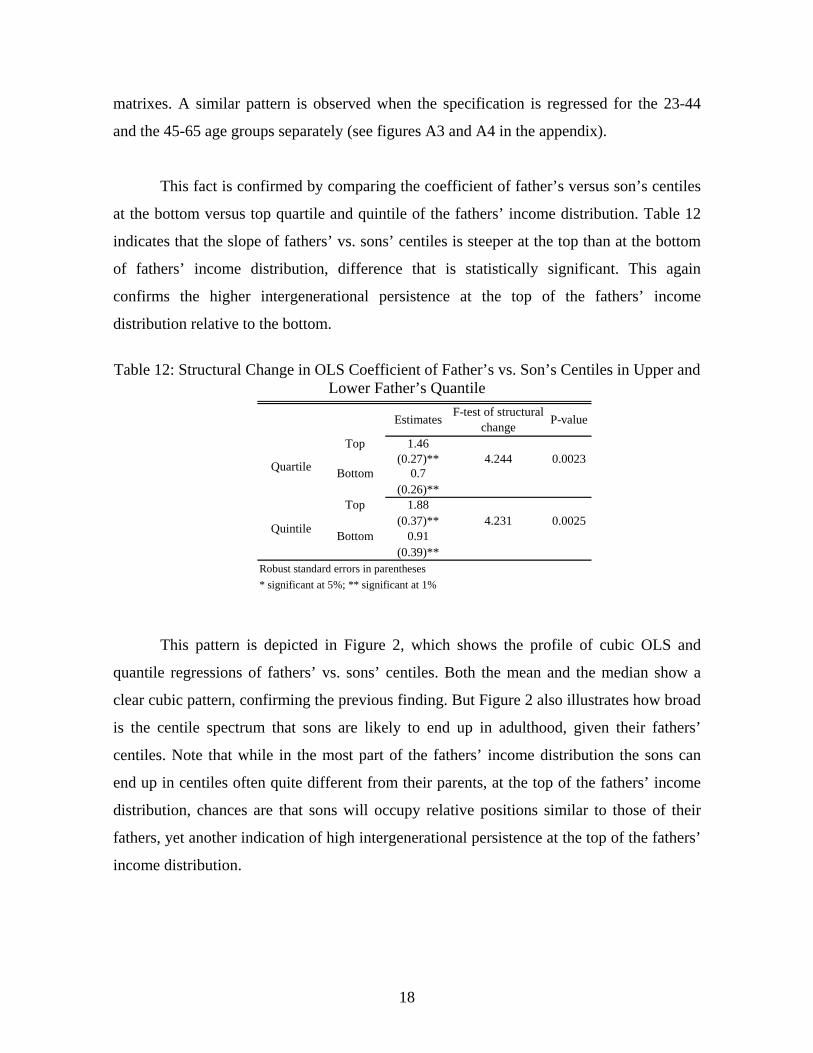
This fact is confirmed by comparing the coefficient of father’s versus son’s centiles

at the bottom versus top quartile and quintile of the fathers’ income distribution. Table 12

indicates that the slope of fathers’ vs. sons’ centiles is steeper at the top than at the bottom

of fathers’ income distribution, difference that is statistically significant. This again

confirms the higher intergenerational persistence at the top of the fathers’ income

distribution relative to the bottom.

Table 12: Structural Change in OLS Coefficient of Father’s vs. Son’s Centiles in Upper and

Lower Father’s Quantile

This pattern is depicted in Figure 2, which shows the profile of cubic OLS and

quantile regressions of fathers’ vs. sons’ centiles. Both the mean and the median show a

clear cubic pattern, confirming the previous finding. But Figure 2 also illustrates how broad

is the centile spectrum that sons are likely to end up in adulthood, given their fathers’

centiles. Note that while in the most part of the fathers’ income distribution the sons can

end up in centiles often quite different from their parents, at the top of the fathers’ income

distribution, chances are that sons will occupy relative positions similar to those of their

fathers, yet another indication of high intergenerational persistence at the top of the fathers’

income distribution.

Estimates F-test of structural change P-value

Top 1.46(0.27)** 4.244 0.0023

Bottom 0.7(0.26)**

Top 1.88(0.37)** 4.231 0.0025

Bottom 0.91(0.39)**

Robust standard errors in parentheses* significant at 5%; ** significant at 1%

Quartile

Quintile

19

Figure 2: Quantile Cubic Regressions

In order to provide another view of the asymmetry between the degrees of

persistence at the tails of the fathers’ income distribution, we have employed the

coefficients of specification 4 of Table 11 in order to obtain the expected son’s income

centile in adulthood, given a level of father’s income centile. From these centiles we have

constructed the expected son’s centile for father’s deciles, which are reported in Table 13.

Table 13: Son’s Expected Centile in Adulthood given Father’s Decile

Table 13 suggests a significant asymmetry in the patterns of mobility in Chile,

which were already suggested by the previous analysis. In fact, the expected centiles of

sons of fathers in the bottom decile is 30, that is, at the border of the 3rd and 4th decile.

Although this shows an important degree of persistence, it also shows an important degree

of the “regression-to-the-mean” effect for this group. Yet, sons of fathers in the top decile

Fathers' Decile Son's Expected Centile (Father's Centile from Real Distribution)

1 30.042 39.903 45.204 47.495 48.356 49.327 51.988 57.889 68.59

10 85.66

0

10

20

30

40

50

60

70

80

90

100

1 4 7 10 14 17 20 23 27 29 33 36 39 42 46 49 52 56 59 62 65 69 72 75 78 82 85 88 92 94 98Father's Centile

Expe

cted

Son

's C

entil

e

90th 75th median mean 25th 10th

20

can expect to be, on average, on the 86th centile, that is well into the 9th decile and close to

the top centile: the “regression-to-the-mean” effect does not seem to be very important in

this case. This pattern repeats in a milder version when comparing the expected centiles of

sons of fathers in the 2nd and 9th deciles, 40 and 69, respectively: the former sons are only

10 centiles below the median, while the latter are 19 centiles above it. As for the sons of

fathers in deciles 3 to 8, their expected centile is only a few percentage points away from

the median, suggesting an important degree of intergenerational income mobility at the

centre of the father’s income distribution. This evidence confirms an important asymmetry

in the patterns of mobility at the extremes of fathers’ income distribution in Chile, with

more relative persistence at the very top than at the very bottom of the fathers’ income

distribution.

Finally, and considering the evidence of a significant amount of intergenerational

persistence in the upper part of the father’s income distribution, we examine how it

compares with the available international evidence. The transition probabilities associated

to the top quintile in Tables 9 and 10 do indeed seem high in comparison with the

international evidence, as shown in Table 14. A similar pattern arises also when comparing

the intergenerational persistence at the top quartile.

Table 14: Comparative evidence on persistence in top quantile

To recap, the evidence suggests three salient features of the patterns of mobility on

Chile. First a higher degree of persistence at the extremes of the fathers’ income

distribution, while substantially more mobility in the intermediate segments of it. Second,

there is evidence of an asymmetry between the degrees of persistence at the bottom versus

the top of fathers’ income distribution, the persistence being higher at the top quantiles.

Study Country Top Quartile Top QuintileVeloso and Ferreira (2004) Brazil 0.43Österberg (2000) Sweden 0.25Peters (1992) U.S. 0.36-0.40Ng (2004) Finland 0.40-0.52Fortin and Lefebvre (1998) Canada 0.32-0.33Nuñez and Risco (2004) Chile 0.50This study Chile 0.55-0.56 0.47-0.57

21

Third, the persistence at the top seems relatively high in comparison with the available

international evidence.

It is interesting to note that the latter two results seem quite consistent with recent

evidence on intergenerational occupational mobility for Chile. In fact, Torche (2005) finds

that Chile exhibits a high level of persistence in the occupations with highest social status

in compassion with the international evidence, but a significant degree of mobility in the

remaining occupations. It seems suggestive that the two investigations based on different

methodologies and different conceptual frameworks reach somewhat converging

conclusions. As a hypothesis awaiting research, this evidence may be associated with

Chile’s particular income distribution, namely the fact that Chile’s income distribution is

unequal for international standards basically due to the large share of the national income

held by the top decile or so of the population, the remaining part of the population being

particularly egalitarian. Put quite simply, perhaps the top decile or so of Chile’s income

distribution is largely responsible for Chile’s unequal distribution of income as well as for

shaping Chile’s social mobility patterns. This hypothesis still awaits explicit investigation.

6. Conclusions

This paper describes some new findings on intergenerational income mobility in

Chile. A shortcoming to study income mobility in Chile is the lack of income panels where

both fathers and their offsprings’ income can be observed. In this context, all the existing

evidence is based on two-sample instrumental variables methodology, where fathers’

income is predicted from income determinants of fathers reported by their sons, such as

schooling, occupation and age.

Yet, by using this methodology, various salient features of intergenerational

mobility can be obtained. First, the available intergenerational income mobility elasticities

for Chile are in the range of 0.52 to 0.67. The figures derived for Greater Santiago are

around 0.52-0.58. Yet these latter figures may underestimate the true nation-wide

elasticities as some parts of the population are left out such as the remote and rural areas,

22

and small urban areas, where intergenerational mobility can be expected to be lower.

However, these figures stand as fairly high in comparison with the international evidence,

mostly for developed countries, but similar to elasticities found for Brazil.

Second, intergenerational income elasticities are somewhat lower for the younger

cohorts. This may suggest an increasing intergenerational mobility in time, although it can

also be associated with life-cycle effects. We also find that educational mobility is lower

for the younger cohorts. We claim that given the fact that schooling remains fixed for most

individuals along the life cycle after the mid twenties, this finding strongly suggests an

increase of intergenerational educational mobility in the last decades. This seems consistent

with the significant expansion of school enrollment and of years of schooling in the last

decades. Whether this has translated into higher intergenerational income mobility is open

for future research.

Third, we also examine how intergenerational mobility varies along the fathers’

relative income position. We find evidence of a high degree of intergenerational persistence

at the bottom-to-bottom and top-to-top transition probabilities, while a significant degree of

mobility in the intermediate segments of the income distribution. Moreover, we find

evidence of an asymmetry in the degrees of persistence between the two tails of the fathers’

income distribution: the intergenerational persistence is higher for the top fathers’ income

quintile or so than for the bottom quintile. The evidence suggests that this high degree of

persistence at the top part of the fathers’ income distribution is large for international

standards, as suggested by the top-to-top transition probabilities. This evidence is consistent

with recent findings of intergenerational occupational mobility for Chile by Torche (2005),

who reports a high degree of persistence in occupations associated with high social status,

but a significant degree of occupational mobility in the rest of the occupations spectrum. It

is tempting to propose, as hypothesis, that this finding may be associated with Chile’s

particular income distribution, quite egalitarian for the 80 to 90 percent of the population,

but rather unequal when the top quintile or decile is considered.

23

An interesting avenue for future research is to study the determinants of

intergenerational and educational mobility in Chile. Although this paper has shed some

light on some patters of Chilean intergenerational income mobility, there is a great deal of

social mobility whose determinants need to be understood. In this respect, the dataset

employed in this paper also includes various measures of circumstances of origin, such as

family background, parental education and functional literacy, parental effort at home,

quality of education, place of origin, ethnicity, among others. Examining the impact of

these factors can shed light on the determinants that can promote more equality of

opportunities.

Finally, more robust and conclusive evidence about intergenerational income

mobility would require establishing proper panels where both parents’ and offsprings’

incomes can be observed. This is certainly a pending issue in Chile as in most developing

countries.

References Abul R. and F. Cowell (2002), “Intergenerational Mobility in Britain: Revisiting the

Prediction Approach of Dearden, Machin and Reed”, Ecole des Hautes Etudes Commerciales. Département D´Econométrie et d´Economie Politique. (disponible en: http://sticerd.lse.ac.uk/dps/darp/darp62.pdf).

Andersen, L. (2000), “Social Mobility in Latin America”, Instituto de Investigaciones

Socio-Económicas Universidad Católica Boliviana. Angrist, J. and A Krueger (1992), “The Effect of Age at School Entry on Educational

Attainment: An Application of Instrumental Variables with Moments from Two Samples”, Journal of American Statistical Association, 87 (418), pp. 328-36.

Arellano, M. and C. Meghir (1992), “Female Labour Supply and On the Job Search: An

Empirical Model Estimated Using Complementary Data Set”, Review of Economic Studies 59(3), pp. 537-59.

Askew D., Brewington, J. and A. Touhey (2001), “An Examination of Intergenerational

Income Mobility Using the Panel Study of Income Dynamics”, Econometrics 375, (in: http://www.ups.edu/econ/pseje/articles/firstedition/atouhey.pdf)

Becker, G. and N. Tomes (1979), “An Equilibrium Theory of the Distribution of Income

and Intergenerational Mobility”, Journal of Political Economy 87, pp. 1153-1189.

24

Björklud, A. and M. Jäntti (1997), “Intergenerational Income Mobility in Sweden

Compared to the United States”, American Economic Review 87(5), pp. 1009-018. Björklud, A. and M. Jäntti (1999), “Intergenerational Mobility of Socio-Economic Status in

Comparative Perspective”, mimeo Stockholm University. Bourguignon, Ferreira and Menendez (2003), “Inequality of Outcomes, Inequality of

Opportunities and Intergenerational Educational Mobility in Brazil”. Washington DC: The World Bank.

Bowles, S. and H. Gintis (2002), “The Inheritance of Inequality”, Journal of Economic

Perspectives 16(3), pp. 3-30. Contreras, D., M. Fuenzalida and J. Nuñez (2006), “Persistencia Intergeneracional del

Ingreso en Chile y el Rol de la Habilidad de los Hijos”, Masters thesis, Economics Department, Universidad de Chile.

Corak, M. and A. Heisz (1999), “The Intergenerational Earnings and Income Mobility of

Canadian Men: Evidence from Longitudinal Income Tax Data”, Journal of Human Resources 34(3), pp. 504-33.

Dahan, M. and A. Gaviria (1999), “Sibling Correlations and Social Mobility in Latin

America”, Inter-American Development Bank, Washington, D.C. Dearden L., Machin S. and H. Reed (1997), “Intergenerational Mobility in Britain”, The

Economic Journal 107(440), pp. 47-66. Dunn, C. (2003), “Intergenerational Earnings Mobility in Brazil” (Paper presented at 8th

annual meeting LACEA). Dunn, C. (2004), “Intergenerational Transmission of Lifetime Earnings: New Evidence

from Brazil”, mimeo Department of Economics and Population Studies Center, University of Michigan.

Ferreira, S. and F. Veloso (2004), “Intergenerational Mobility of Wages in Brazil”.

Unpublished paper. Fields, G. (2001), “Distribution and Development. A New look at the developing world”,

Russell Sage Foundation and MIT Press. Fortín, N. and S. Lefebvre (1998), “Intergenerational Income Mobility in Canada”, Labor

Markets, Social Institutions, and the Future of Canada’s Children. Hertz, T. (2001), “Education, Inequality and Economic Mobility in South Africa”, Ph.D.

thesis, University of Massachusetts.

25

Lefrane A. and A. Trannoy (2004), “Intergenerational Earnings mobility in France: Is France more mobile than the US?”, Accepté dans Annales d`Economie et de Statistiques.

Lillard, L. and M. Kilburn (1995), “Intergenerational Earnings Links: Sons and Daughters”,

unpublished paper. Nuñez, J. and C. Risco (2004), “Movilidad Intergeneracional de Ingresos en un País en

Desarrollo: El Caso de Chile”, Working Paper N° 210, Department of Economics, Universidad de Chile.

Nuñez, J. and R. Gutiérrez (2004), “Classism, Meritocracy and Discrimination in the Labor

Market: The case of Chile”, Working Paper N° 208, Department of Economics, Universidad de Chile.

Nuñez, J. and A. Tartakowsky (2006), “Inequality of Outcomes vs. Inequality of

Opportunities in Chile”, mimeo, Department of Economics, Universidad de Chile. Österbacka, E. (2001), “Family Background and Economic Status in Finland”, Scand J. of

Economics 103(3), pp. 467-484. Peters, E. (1992), “Patterns of Intergenerational Mobility in Income and Earnings”, The

Review of Economics and Statistics 74, pp. 456-466. Solon, G. (1992), “Intergenerational Income Mobility in the United States”, The American

Economic Review 82(3), pp. 393-408. Solon, G. (2002), “Cross-countries Differences in Intergenerational Earnings Mobility”,

The Journal of Economic Perspectives 16(3), pp. 59-66. Torche, F. (2005), “Unequal but fluid: social mobility in Chile in comparative perspective”,

American Sociological Review 70(3), pp. 422-450. Wiegand, J. (1997), “Intergenerational Earnings Mobility in Germany”, unpublished paper. Zimmerman, D. (1992), “Regression toward Mediocrity in Economic Stature”, The

American Economic Review 82, pp. 409-429.

26

Appendix

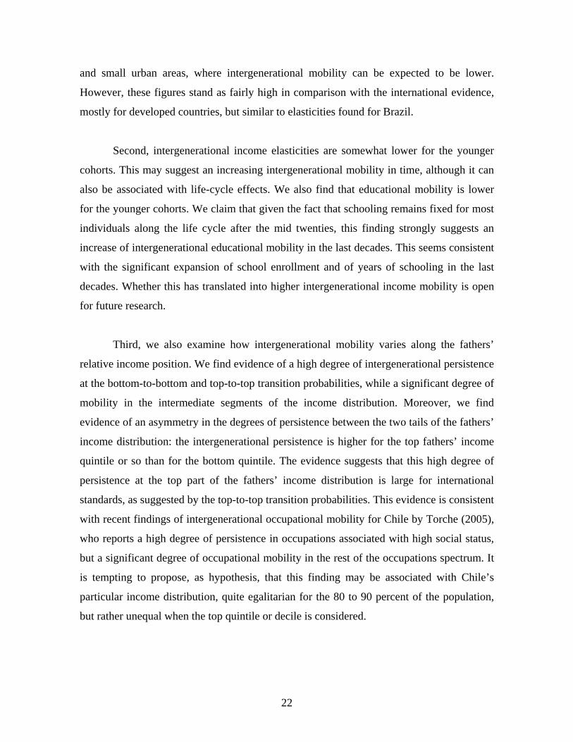
Table A.1: Estimates of Mincer equations using education and potential experience as regressors

Table A.2: Estimates of Mincer equations using education, potential experience and occupation as regressors

Log Income Personal Income Labor Income Personal Income Labor Income Personal Income Labor Income Personal Income Labor IncomeS 0.1098 0.1043 0.0768 0.0725 0.0784 0.0808 0.0638 0.0626

(14.76)** (14.20)** (11.38)** (10.78)** (8.35)** (8.60)** (5.59)** (5.43)**(S-8)*d1 0.0839 0.0873 0.1252 0.1288 0.1266 0.1240 0.1038 0.1066

(4.73)** (4.99)** (8.71)** (8.98)** (7.20)** (7.04)** (5.55)** (5.65)**(S-12)*d2 -0.0675 -0.0722 -0.0249 -0.0329 -0.0322 -0.0343 0.1152 0.1112

(3.00)** (3.25)** (1.54) (2.04)* (1.88) (2.01)* (7.19)** (6.89)**Exper 0.0604 0.0605 0.0620 0.0617 0.0636 0.0651 0.0539 0.0545

(14.20)** (14.43)** (18.73)** (18.63)** (16.60)** (17.00)** (13.11)** (13.17)**Exper2 -0.0008 -0.0009 -0.0009 -0.0009 -0.0009 -0.0009 -0.0007 -0.0007

(10.47)** (11.14)** (13.79)** (14.12)** (11.52)** (12.33)** (7.87)** (8.23)**Constant 8.9524 8.9958 11.4925 11.5125 6.0278 5.9930 8.3213 8.3199

(134.89)** (137.61)** (210.52)** (211.27)** (79.81)** (79.34)** (92.97)** (92.11)**Observations 1747 1736 2700 2691 2325 2321 2070 2068Adj. R-squared 0.51 0.50 0.53 0.52 0.48 0.48 0.59 0.59Absolute value of t statistics in parentheses* significant at 5%; ** significant at 1%

1958 1967 1977 1987

Log Income Personal Income Labor Income Personal Income Labor Income Personal Income Labor Income Personal Income Labor IncomeS 0.0852 0.0805 0.0526 0.0478 0.0584 0.0606 0.0511 0.0499

(11.46)** (10.97)** (7.84)** (7.16)** (6.59)** (6.87)** (4.94)** (4.77)**(S-8)*d1 0.0496 0.0530 0.1033 0.1087 0.0808 0.0759 0.0629 0.0646

(2.89)** (3.12)** (7.47)** (7.89)** (4.87)** (4.58)** (3.64)** (3.71)**(S-12)*d2 -0.0083 -0.0127 0.0199 0.0100 0.0195 0.0196 0.1418 0.1383

(0.38) (0.58) (1.26) (0.64) (1.21) (1.22) (9.73)** (9.42)**Exper 0.0548 0.0550 0.0550 0.0545 0.0527 0.0538 0.0427 0.0432

(13.37)** (13.59)** (17.16)** (17.10)** (14.57)** (14.96)** (11.32)** (11.38)**Exper2 -0.0008 -0.0008 -0.0008 -0.0008 -0.0007 -0.0008 -0.0005 -0.0006

(10.30)** (10.90)** (13.17)** (13.52)** (10.48)** (11.29)** (6.94)** (7.34)**Employer=1 0.7414 0.7137 1.0662 1.0558 1.3777 1.4163 1.5265 1.5306

(10.82)** (10.49)** (15.37)** (15.23)** (18.79)** (19.29)** (21.22)** (21.12)**Self-employed=1 0.1677 0.1220 0.2197 0.2033 0.2582 0.2637 0.0983 0.0994

(4.44)** (3.27)** (6.69)** (6.21)** (7.16)** (7.35)** (2.71)** (2.72)**Employee=1 0.3755 0.3734 0.2997 0.2962 0.3794 0.3891 0.3284 0.3389

(9.96)** (10.05)** (9.95)** (9.87)** (10.59)** (10.89)** (9.08)** (9.30)**Domestic servants=1 -0.7535 -0.7570 -0.3714 -0.7523 0.0025 -0.3188 - -

(1.97)* (2.01)* (1.89) (3.85)** (0.01) (0.91) - -Constant 9.0698 9.1128 11.6337 11.6607 6.1962 6.1659 8.5123 8.5107

(141.07)** (143.92)** (219.63)** (221.22)** (87.39)** (87.34)** (104.32)** (103.31)**Observations 1747 1736 2700 2691 2325 2321 2070 2068Adj. R-squared 0.55 0.54 0.58 0.57 0.55 0.56 0.67 0.66

Absolute value of t statistics in parentheses* significant at 5%; ** significant at 1%

1958 1967 1977 1987

27

Table A3: Quartile Transition Matrix

Table A4: Quartile Transition Matrix Father’s quartile from distribution of predicted income

Father Bottom 2nd 3rd TopBottom 0.50 0.27 0.19 0.04

2nd 0.30 0.22 0.33 0.153rd 0.29 0.24 0.28 0.19Top 0.14 0.14 0.18 0.54

Immobility Index 0.38

Son

Father's quartile from real income distribution

Father Bottom 2nd 3rd TopBottom 0.39 0.24 0.30 0.08

2nd 0.32 0.23 0.30 0.153rd 0.26 0.26 0.22 0.26Top 0.12 0.12 0.20 0.55

Immobility Index 0.35

Son

28

Figure A1: Intergenerational Income Transition Probabilities (Quintiles)

Figure A2: Intergenerational Income Transition Probabilities (Quartiles)

Bottom2nd

3rd4th

Top

Bottom2nd

3rd

4th

Top

0.00

0.10

0.20

0.30

0.40

0.50

0.60

Son's QuintileFather's Quintile

Probability Son from HighestIncome Quintile Family is in Highest Quintile is 47%

Probability Son from Lowest Income Quintile Family is in Lowest Quintile is 37%

Lowest Quintile Father, Highest Quintile Son, 0%

Highest Quintile Father, Lowest Quintile Son, 8%

AB

C D

Bottom2nd

3rdTop

Bottom

2nd

3rd

Top

0.00

0.10

0.20

0.30

0.40

0.50

0.60

Son's Quartil

Father's Quartil

Probability Son from Lowest Income Quartile Family is in Lowest Quartile is 50%

Probability Son from HighestIncome Quartile Family is in Highest Quartile is 54%

Lowest Quartile Father, Highest Quartile Son, 4%

Highest Quartile Father, Lowest Quartile Son, 14%

A

B

CD

29

Figure A3: Quantile Cubic Regressions for 23-44 cohort

Figure A4: Quantile Cubic Regressions for 45-65 cohort

0102030405060708090

100

1 5 10 15 19 24 29 34 39 44 48 53 58 62 67 73 77 82 87 92 96Father's Centile

Expe

cted

Son

's C

entil

e

90th 75th median mean 25th 10th

0102030405060708090

100

1 5 10 15 21 26 31 35 41 46 51 56 62 67 72 77 82 87 92 98Father's Centile

Expe

cted

Son

's C

entil

e

90th 75th median mean 25th 10th