Lucio Torrisi and Francesca Marcucci

CNMCA, Italian National Met Center

Recent developments for CNMCA LETKF

Outline

Implementation of the LETKF at CNMCA

Treatment of model error in the CNMCA-LETKF

The Self Evolving Additive Noise: different formulations

Forecast verification over 30-days test period

Test with the recent version of the SPPT

Assimilation of new observations (ATMS and GPS)

Summary and future developments

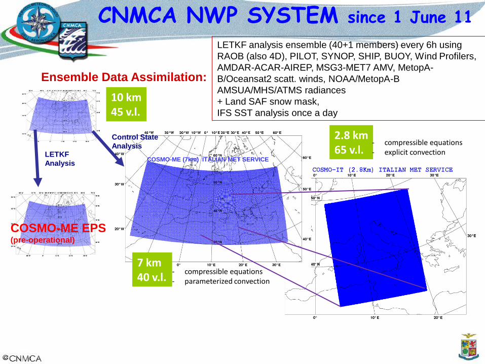
2.8 km65 v.l.

- compressible equations- explicit convection

CNMCA NWP SYSTEM since 1 June 11

LETKF analysis ensemble (40+1 members) every 6h using

RAOB (also 4D), PILOT, SYNOP, SHIP, BUOY, Wind Profilers,

AMDAR-ACAR-AIREP, MSG3-MET7 AMV, MetopA-

B/Oceansat2 scatt. winds, NOAA/MetopA-B

AMSUA/MHS/ATMS radiances

+ Land SAF snow mask,

IFS SST analysis once a day

Ensemble Data Assimilation:

COSMO-ME (7km) ITALIAN MET SERVICE

10 km45 v.l.

Control State

Analysis

COSMO-ME EPS(pre-operational)

LETKF

Analysis

7 km40 v.l.

- compressible equations- parameterized convection

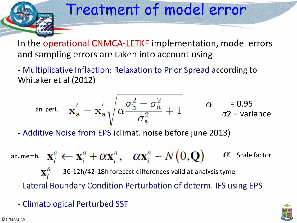
Treatment of model error

Scale factor

36-12h/42-18h forecast differences valid at analysis tyme

= 0.95σ2 = variance

In the operational CNMCA-LETKF implementation, model errors and sampling errors are taken into account using:

an. pert.

an. memb.

- Multiplicative Inflaction: Relaxation to Prior Spread according to Whitaker et al (2012)

- Additive Noise from EPS (climat. noise before june 2013)

- Lateral Boundary Condition Perturbation of determ. IFS using EPS

- Climatological Perturbed SST

Additive Noise from IFS

The additive noise derived from IFS model is not consistent

with COSMO model errors statistics, but it may temporarily

substitute the climatological one (avoiding a decrease of the

spread in the CNMCA COSMO-LETKF).

First (!not last) solution:

AIM: Find additive perturbations that are both consistent

with model errors statistics and a flow-dependent noise

Self-Evolving Additive Noise

The self-evolving additive inflaction (idea of Mats Hamrud – ECMWF) is

chosen. The idea is different from that of the evolved additive noise of

Hamill and Whitaker (2010)

• The dfference between ensemble forecasts valid at the analysis time

is calculated. The mean difference is then subtracted to yield a set of

perturbations that are scaled and used as additive noise. The ensemble

forecasts are obtained by the same ensemble DA system extending

the end of the model integration.

• This can be considered as a blending” of two set of perturbations, that

should increase the “dimension” of the ensemble (i.e. 6h and 12h

perturbations)

• The error introduced during the first hours may have a component that

will project onto the growing forecast structures having probably a

benificial impact on spread growth and ensemble-mean error

Self-Evolving Additive Noise

AN -1

AN -2

AN -N FC -N

AN -1

AN -2

AN -N FC -N

FC -2

FC -1

FC -2

FC -1

AN -1

AN -2

AN -N FC -N

AN -1

AN -2

AN -N

FC -2

FC -1

t

+6hAdditive

noise valid

at t

+6h

+6h

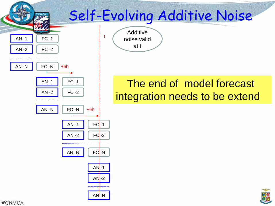
The end of model forecast

integration needs to be extend

Self-Evolving Additive Noise

AN -1

AN -2

AN -N FC -N

FC -2

FC -1

AN -1

AN -2

AN -N FC -N

FC -2

FC -1

AN -1

AN -2

AN -N FC -N

FC -2

FC -1

AN -1

AN -2

AN -N

Additive

noise valid

at t

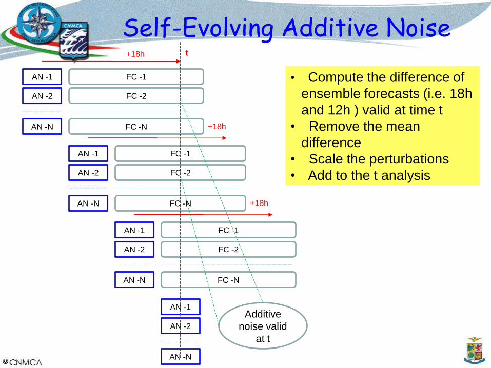
• Compute the difference of

ensemble forecasts (i.e. 18h

and 12h ) valid at time t

• Remove the mean

difference

• Scale the perturbations

• Add to the t analysis

t+18h

+18h

+18h

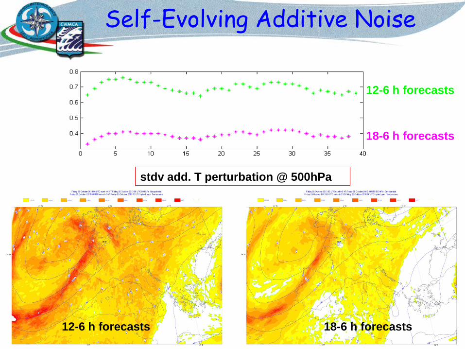
Self-Evolving Additive Noise

stdv add. T perturbation @ 500hPa

Features of first version:

12h-6h forecast differences

Spatial filtering of ensemble difference using a low pass 10th order

Raymond filter

Adaptive scaling factor using the surface pressure obs inc statistics R=0

PERTPS

To

b

o

b HBHRddE

_

][

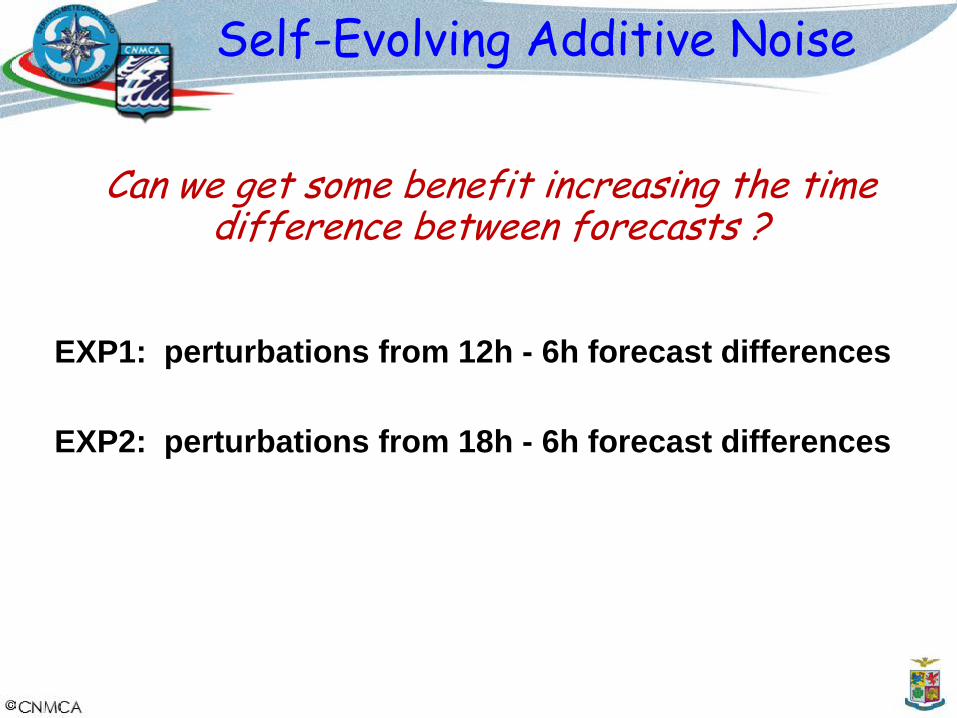
Can we get some benefit increasing the time difference between forecasts ?

Self-Evolving Additive Noise

EXP2: perturbations from 18h - 6h forecast differences

EXP1: perturbations from 12h - 6h forecast differences

Self-Evolving Additive Noise

12-6 h forecasts

18-6 h forecasts

stdv add. T perturbation @ 500hPa

12-6 h forecasts 18-6 h forecasts

Obs Increment Statistics

OBS INCREMENT ON MODEL

LEVELS (TEMP + RAOB obs)

18-6h VS 12-6h

21 oct 2013 – 10 nov 2013

Forecast verification

Relative difference (%) in RMSE,

computed against IFS analysis, with respect

to NO-ADDITIVE run

for 00 UTC COSMO runs from

21-oct 2013 to 10 nov 2013

negative value = positive impact

+12h +24h +36h +48h +12h +24h +36h +48h

+12h +24h +36h +48h

Self-Evolving Additive Noise

PERTPS

To

b

o

b HBHRddE

_

][

EXP1: R = 0, perturbations from 12h - 6h forecast differences

EXP3: R = 0.3, perturbations from 12h - 6h forecast differences

Experiments on estimation of scaling factor

EXP4: as EXP3 with temporal smoothing at same time (00,06,12,18 UTC)

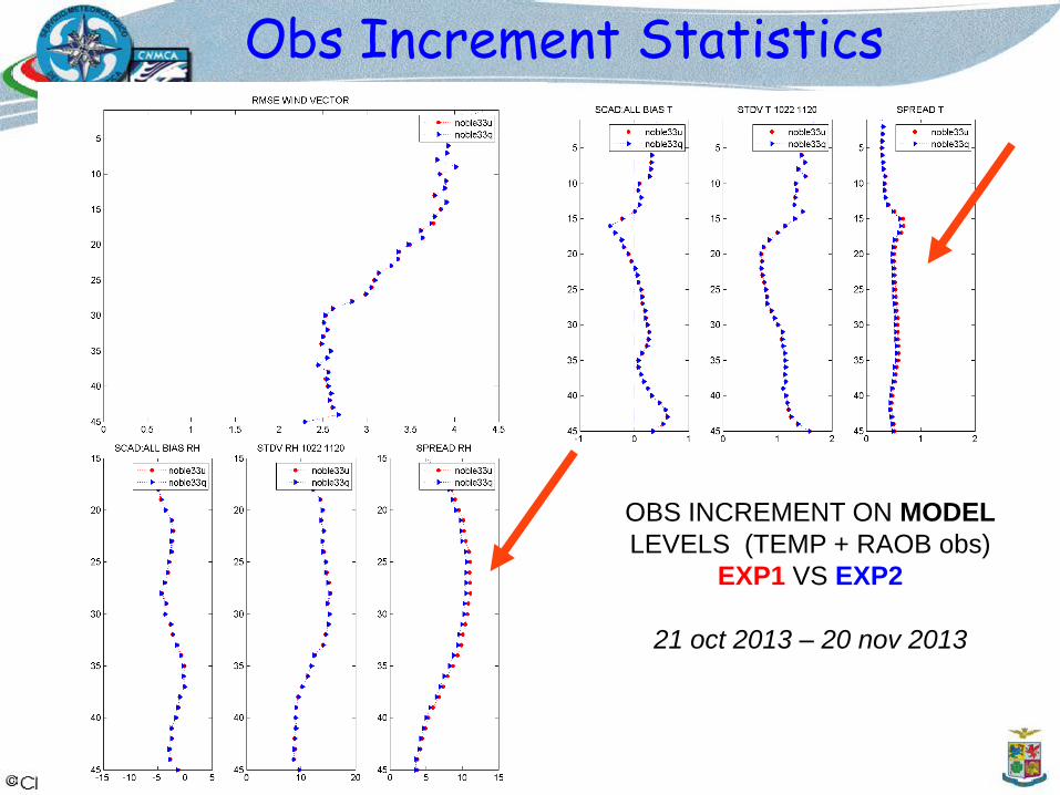
Obs Increment Statistics

OBS INCREMENT ON MODEL

LEVELS (TEMP + RAOB obs)

EXP1 VS EXP2

21 oct 2013 – 20 nov 2013

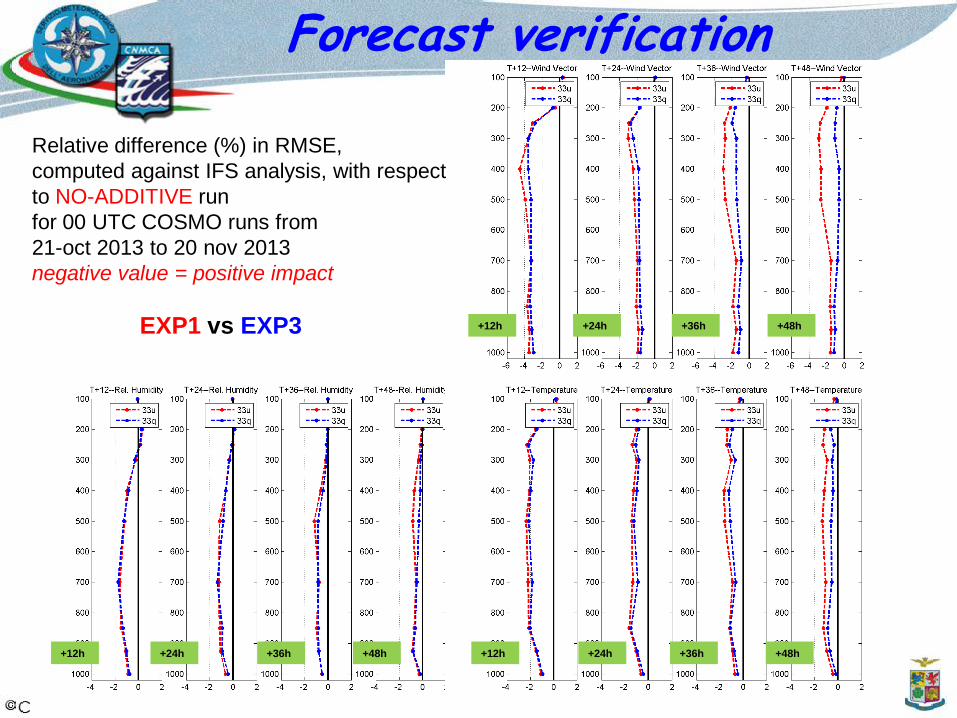
Forecast verification

+12h +24h +36h +48h +12h +24h +36h +48h

+12h +24h +36h +48h

Relative difference (%) in RMSE,

computed against IFS analysis, with respect

to NO-ADDITIVE run

for 00 UTC COSMO runs from

21-oct 2013 to 20 nov 2013

negative value = positive impact

EXP1 vs EXP3

Forecast Verification

Relative difference (%) in RMSE,

computed against IFS analysis, with respect

to NO-ADDITIVE runfor 00 UTC COSMO runs from22 oct 2013 – 10 nov 2013

negative value = positive impact

+12h +24h +36h +48h

+12h +24h +36h +48h+12h +24h +36h +48h

DAY2DAY1

EPS, EXP1, EXP4

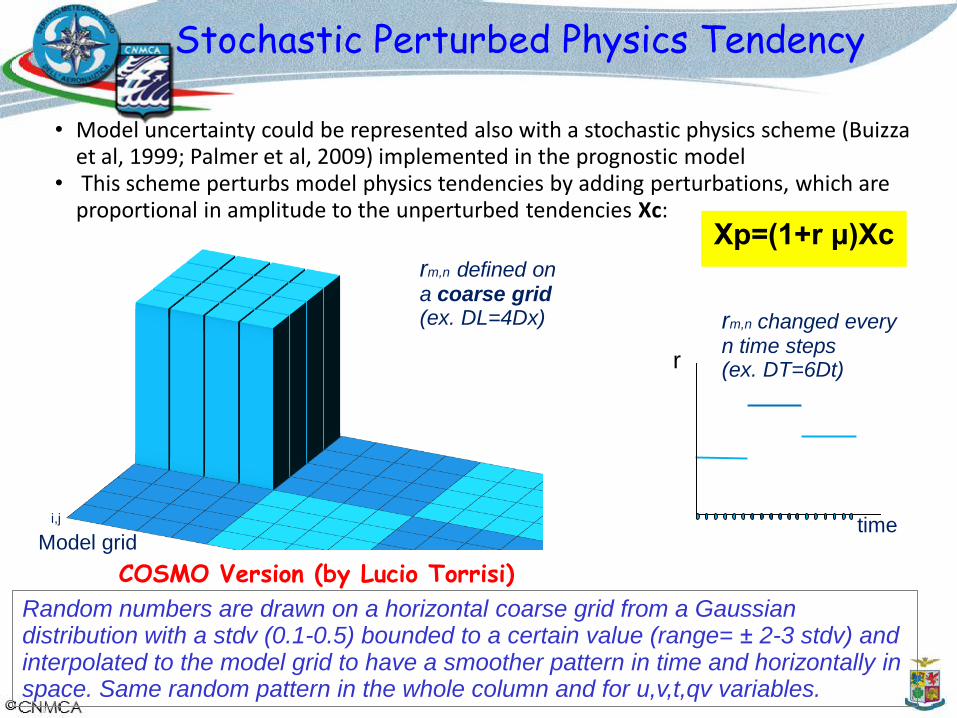
• Model uncertainty could be represented also with a stochastic physics scheme (Buizza et al, 1999; Palmer et al, 2009) implemented in the prognostic model

• This scheme perturbs model physics tendencies by adding perturbations, which are proportional in amplitude to the unperturbed tendencies Xc:

rm,n defined on a coarse grid(ex. DL=4Dx)

i,j

Model grid

r

time

rm,n changed everyn time steps (ex. DT=6Dt)

COSMO Version (by Lucio Torrisi)

Random numbers are drawn on a horizontal coarse grid from a Gaussian distribution with a stdv (0.1-0.5) bounded to a certain value (range= ± 2-3 stdv) and interpolated to the model grid to have a smoother pattern in time and horizontally in space. Same random pattern in the whole column and for u,v,t,qv variables.

Xp=(1+r μ)Xc

Stochastic Perturbed Physics Tendency

OBS INCREMENT STATISTICS (RAOB)STOCHASTIC PHYSICS VS SELF-EVOLVING ADDITIVE

22 OCT 2013 – 20 NOV 2013

The most recent version of SPPT is slightly better than the old one. SPPT seems to have a neutral/little negative impact if used in combination with self ev. add.

Forecast Verification

Relative difference (%) in RMSE, computed against IFS analysis, with respect to

SELF EVOLV ADD run for 00 UTC COSMO runs from 22 OCT–10 NOV 2013

negative value = positive impact

SPPT SETTINGS:stdv=0.4, range=0.8box 5° x 5°, 6 hourinterp. in space and timeno humidity checkT U V qv tendenciesNo tapering near surfaceIMODE_RN=1 (=0 FOR OLD)

NEWvs

OLD

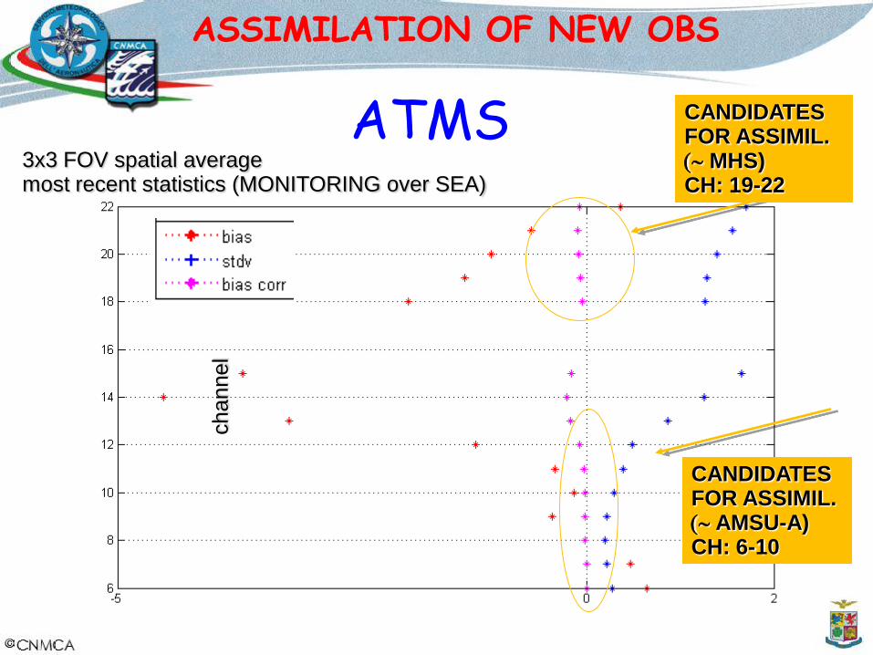
ASSIMILATION OF NEW OBS

3x3 FOV spatial averagemost recent statistics (MONITORING over SEA)

channel

CANDIDATES FOR ASSIMIL. MHS)CH: 19-22

CANDIDATES FOR ASSIMIL. AMSU-A)CH: 6-10

ATMS

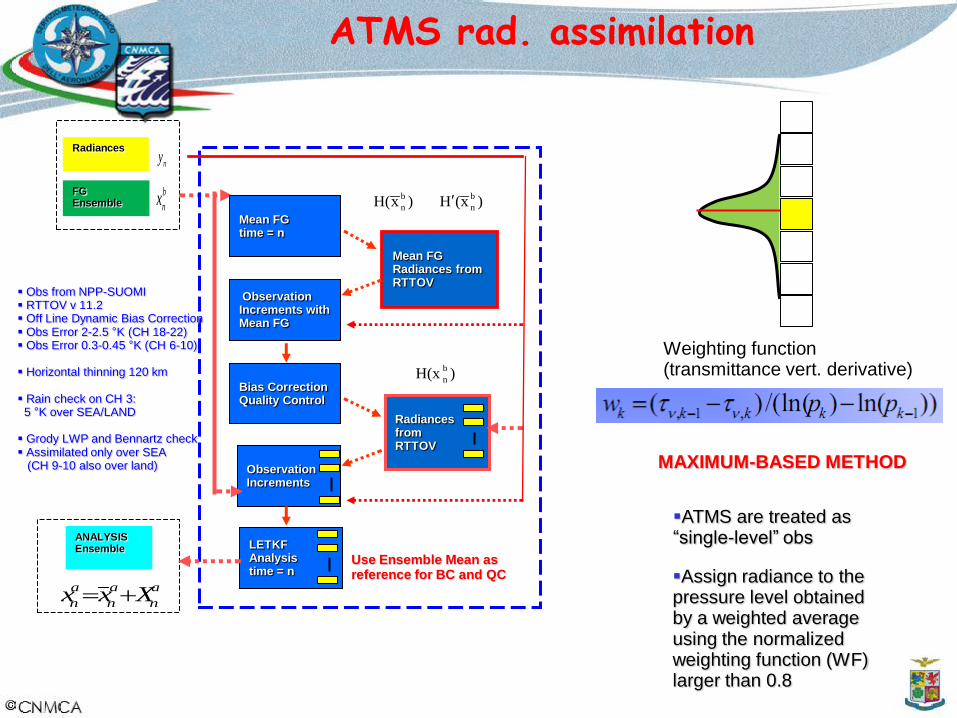
MAXIMUM-BASED METHOD

ATMS are treated as “single-level” obs

Assign radiance to the pressure level obtained by a weighted average using the normalized weighting function (WF) larger than 0.8

Radiances from RTTOV

ny

Mean FG time = n

Bias CorrectionQuality Control

Observation Increments

a a a

n n nx x X

Mean FG Radiances from RTTOV

Observation Increments withMean FG

LETKF Analysis time = n

Radiances

FG Ensemble

b

nx

ANALYSIS Ensemble

Obs from NPP-SUOMI RTTOV v 11.2 Off Line Dynamic Bias Correction Obs Error 2-2.5 °K (CH 18-22) Obs Error 0.3-0.45 °K (CH 6-10)

Horizontal thinning 120 km

Rain check on CH 3:5 °K over SEA/LAND

Grody LWP and Bennartz check Assimilated only over SEA

(CH 9-10 also over land)

Use Ensemble Mean as reference for BC and QC

)x(Hb

n)xH(

b

n

)H(xb

n

ATMS rad. assimilation

Weighting function (transmittance vert. derivative)

Observation Increments Statistics from 12 aug 2014 to 3 sept 2014 (asimilated over SEA, channel 9-10 also over land)

Obs Increment Statistics

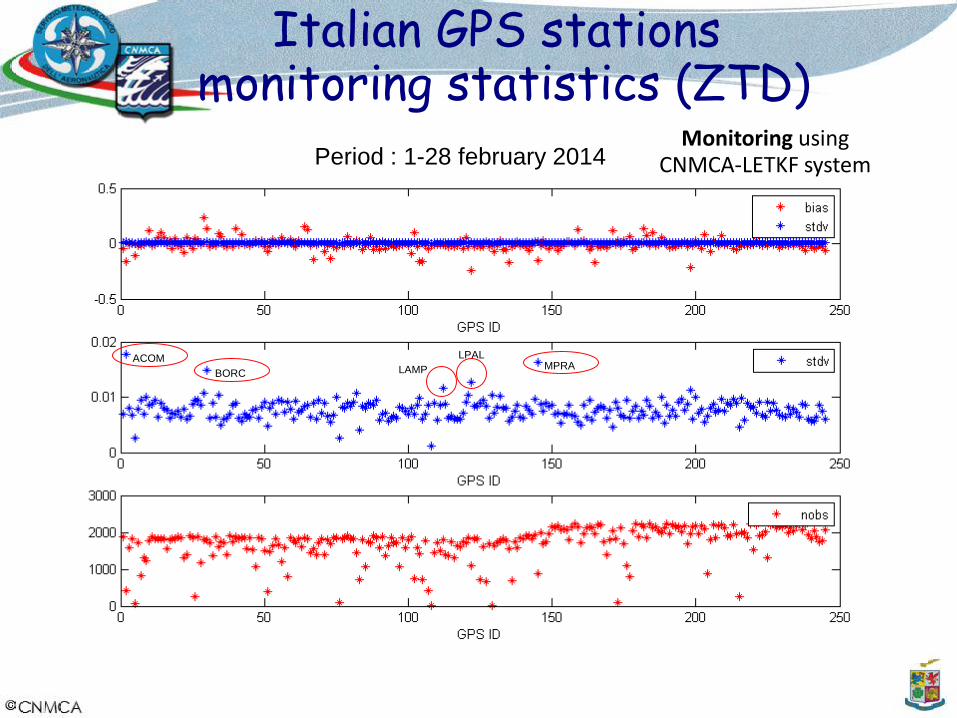
Italian GPS stationsmonitoring statistics (ZTD)

Period : 1-28 february 2014

BORCMPRALAMP

LPALACOM

Monitoring using CNMCA-LETKF system

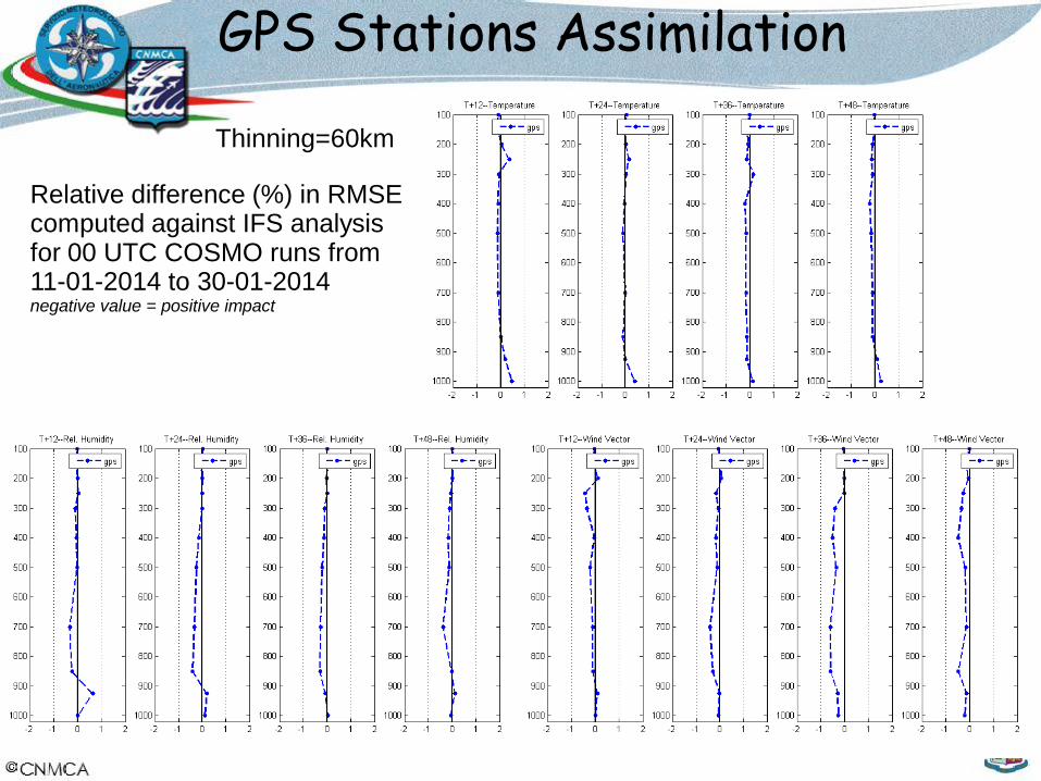
GPS Stations Assimilation

Relative difference (%) in RMSEcomputed against IFS analysisfor 00 UTC COSMO runs from11-01-2014 to 30-01-2014negative value = positive impact

Thinning=60km

Summary and future steps

-“Self evolving additive noise” perturbations are both consistent

with model errors statistics and a flow-dependent noise

- Additive noise computed using differences of forecasts with

larger time distance (i.e. 18-6h) is computationally expensive

and does not improve the scores

- Further tuning of the 12-6 h forecast (filter and scaling factor) is

planned

-A combination of self evolving additive noise and SPPT has

been tested, but no impact is obtained (further tuning!)

- ATMS obs are already operationally assimilated, as soon as

possible also GPS (bias corrected)

- On november (??) the EUMETSAT fellowship will start … first

test of KENDA!

Thanks for your attention!