
Statistical Physics of Fracture: Recent Advances through High-Performance Computing
Recent Advances in Post-Selection StatisticalInference
Robert Tibshirani, Stanford University
December 9, 2015
Breiman lecture, NIPS 2015
Joint work with Jonathan Taylor, Richard Lockhart, RyanTibshirani, Will Fithian, Jason Lee, Yuekai Sun, Dennis Sun,Yun Jun Choi, Max G’Sell, Stefan Wager, AlexChouldechova
Thanks to Jon, Ryan & Will for help with the slides.
1 / 46

My history
I PhD Statistics 1984 (Stanford); went home to University ofToronto (Biostatistics & Statistics)
I Met Geoff Hinton
I and Zoubin Ghahramani, Carl Rasmussen, Rich Zemel,Radford Neal, Brendan Frey, Peter Dayan
I They were fitting models with more parameters thanobservations!!
2 / 46

My history at NIPS
I Starting in the early 90’s, attended pretty regularly with LeoBreiman, Jerry Friedman & Trevor Hastie.
I A few hundred people; The Statisticians were minorcelebrities; “easy” to get a poster accepted.
I Jerry: “The currency is ideas!”
I But I haven’t been for about 15 years
3 / 46

My recent experience:
I Submitted papers to NIPS. No luck
I Tried again No luck
I Tried yet again No luck
I Gave up
I
I
I Got invited! (because I’m getting old?)
4 / 46

My recent experience:
I Submitted papers to NIPS.
No luck
I Tried again No luck
I Tried yet again No luck
I Gave up
I
I
I Got invited! (because I’m getting old?)
4 / 46

My recent experience:
I Submitted papers to NIPS. No luck
I Tried again No luck
I Tried yet again No luck
I Gave up
I
I
I Got invited! (because I’m getting old?)
4 / 46

My recent experience:
I Submitted papers to NIPS. No luck
I Tried again
No luck
I Tried yet again No luck
I Gave up
I
I
I Got invited! (because I’m getting old?)
4 / 46

My recent experience:
I Submitted papers to NIPS. No luck
I Tried again No luck
I Tried yet again No luck
I Gave up
I
I
I Got invited! (because I’m getting old?)
4 / 46

My recent experience:
I Submitted papers to NIPS. No luck
I Tried again No luck
I Tried yet again
No luck
I Gave up
I
I
I Got invited! (because I’m getting old?)
4 / 46

My recent experience:
I Submitted papers to NIPS. No luck
I Tried again No luck
I Tried yet again No luck
I Gave up
I
I
I Got invited! (because I’m getting old?)
4 / 46

My recent experience:
I Submitted papers to NIPS. No luck
I Tried again No luck
I Tried yet again No luck
I Gave up
I
I
I Got invited! (because I’m getting old?)
4 / 46

My recent experience:
I Submitted papers to NIPS. No luck
I Tried again No luck
I Tried yet again No luck
I Gave up
I
I
I Got invited! (because I’m getting old?)
4 / 46

My recent experience:
I Submitted papers to NIPS. No luck
I Tried again No luck
I Tried yet again No luck
I Gave up
I
I
I Got invited! (because I’m getting old?)
4 / 46

My recent experience:
I Submitted papers to NIPS. No luck
I Tried again No luck
I Tried yet again No luck
I Gave up
I
I
I Got invited!
(because I’m getting old?)
4 / 46

My recent experience:
I Submitted papers to NIPS. No luck
I Tried again No luck
I Tried yet again No luck
I Gave up
I
I
I Got invited! (because I’m getting old?)
4 / 46

This talk is about Statistical Inference
Construction of p-values and confidence intervals for modelsand parameters fit to data
Frequentist (non-Bayesian) framework
The word “deep” appears only once in what follows. ($5 U.S tothe person who spots it first)
5 / 46

Statistics versus Machine Learning
How statisticians see the world?
6 / 46

Statistics versus Machine Learning
How machine learners see the world?
6 / 46

Quoting Leo
Statistical Science2001, Vol. 16, No. 3, 199–231
Statistical Modeling: The Two CulturesLeo Breiman
Abstract. There are two cultures in the use of statistical modeling toreach conclusions from data. One assumes that the data are generatedby a given stochastic data model. The other uses algorithmic models andtreats the data mechanism as unknown. The statistical community hasbeen committed to the almost exclusive use of data models. This commit-ment has led to irrelevant theory, questionable conclusions, and has keptstatisticians from working on a large range of interesting current prob-lems. Algorithmic modeling, both in theory and practice, has developedrapidly in fields outside statistics. It can be used both on large complexdata sets and as a more accurate and informative alternative to datamodeling on smaller data sets. If our goal as a field is to use data tosolve problems, then we need to move away from exclusive dependenceon data models and adopt a more diverse set of tools.
1. INTRODUCTION
Statistics starts with data. Think of the data asbeing generated by a black box in which a vector ofinput variables x (independent variables) go in oneside, and on the other side the response variables ycome out. Inside the black box, nature functions toassociate the predictor variables with the responsevariables, so the picture is like this:
y xnature
There are two goals in analyzing the data:
Prediction. To be able to predict what the responsesare going to be to future input variables;Information. To extract some information abouthow nature is associating the response variablesto the input variables.
There are two different approaches toward thesegoals:
The Data Modeling Culture
The analysis in this culture starts with assuminga stochastic data model for the inside of the blackbox. For example, a common data model is that dataare generated by independent draws from
response variables = f(predictor variables,random noise, parameters)
Leo Breiman is Professor, Department of Statistics,University of California, Berkeley, California 94720-4735 (e-mail: [email protected]).
The values of the parameters are estimated fromthe data and the model then used for informationand/or prediction. Thus the black box is filled in likethis:
y xlinear regression logistic regressionCox model
Model validation. Yes–no using goodness-of-fittests and residual examination.Estimated culture population. 98% of all statisti-cians.
The Algorithmic Modeling Culture
The analysis in this culture considers the inside ofthe box complex and unknown. Their approach is tofind a function f!x"—an algorithm that operates onx to predict the responses y. Their black box lookslike this:
y xunknown
decision treesneural nets
Model validation. Measured by predictive accuracy.Estimated culture population. 2% of statisticians,many in other fields.
In this paper I will argue that the focus in thestatistical community on data models has:
• Led to irrelevant theory and questionable sci-entific conclusions;
199
There are two cultures in the use of statistical modeling to reachconclusions from data. One assumes that the data are generatedby a given stochastic data model. The other uses algorithmicmodels and treats the data mechanism as unknown. Thestatistical community has been committed to the almost exclusiveuse of data models. This commitment has led to irrelevanttheory, questionable conclusions, and has kept statisticians fromworking on a large range of interesting current problems.
7 / 46
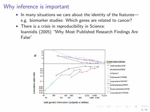
Why inference is importantI In many situations we care about the identity of the features—
e.g. biomarker studies: Which genes are related to cancer?I There is a crisis in reproducibility in Science:
Ioannidis (2005) “Why Most Published Research Findings AreFalse”
Figure 2: Cumulative odds ratio as a function of total genetic information as determined bysuccessive meta-analyses. a) Eight cases in which the final analysis di↵ered by more thanchance from the claims of the initial study. b) Eight cases in which a significant associationwas found at the end of the meta-analysis, but was not claimed by the initial study. FromIoannidis et al. 2001.
true null hypotheses (R) decreases, the FDR will increase.Moreover, the e↵ect of bias can alter this dramatically. For simplicity, Ioannidis models
all sources of bias as a single factor u, which is the proportion of null hypotheses that wouldnot have been claimed as discoveries in the absence of bias, but which ended up as suchbecause of bias. There are many sources of bias which will be discussed in greater detail insection 2.3.
The e↵ect of this bias is to modify the equation for PPV to be:
PPV = 1 � FDR =(1 � �)R + u�R
(1 � �)R + u�R + ↵ + u(1 � ↵)
4
8 / 46

The crisis- continued
I Part of the problem is non-statistical- e.g. incentives forauthors or journals to get things right.
I But part of the problem is statistical– we search throughlarge number of models to find the “best” one; we don’t havegood ways of assessing the strength of the evidence
I today’s talk reports some progress on the development ofstatistical tools for assessing the strength of evidence, aftermodel selection
9 / 46

Our first paper on this topic: An all “Canadian” team
Richard Lockhart Jonathan Taylor Simon Fraser University !!!!!!!!!!!!!!!!Stanford!University!
Vancouver !!!!!!!!!!PhD!Student!of!Keith!Worsley,!2001!PhD . Student of David Blackwell, !
Berkeley,!1979!!
Ryan Tibshirani , CMU. PhD student of Taylor 2011
Rob Tibshirani Stanford
10 / 46

Fundamental contributions by some terrific students!
Will Fithian Jason Lee Yuekai Sun UC BERKELEY
Max G’Sell, CMU Dennis Sun-‐ Google Xiaoying Tian, Stanford
Yun Jin Choi Stefan Wager Alex Chouldchova Josh Loftus Now at CMU STANFORD
11 / 46

Some key papers in this work
I Lockhart, Taylor, Tibs & Tibs. A significance test for thelasso. Annals of Statistics 2014
I Lee, Sun, Sun, Taylor (2013) Exact post-selection inferencewith the lasso. arXiv; To appear
I Fithian, Sun, Taylor (2015) Optimal inference after modelselection. arXiv. Submitted
I Tibshirani, Ryan, Taylor, Lockhart, Tibs (2016) ExactPost-selection Inference for Sequential RegressionProcedures. To appear, JASA
I Tian, X. and Taylor, J. (2015) Selective inference with arandomized response. arXiv
I Fithian, Taylor, Tibs, Tibs (2015) Selective SequentialModel Selection. arXiv Dec 2015
12 / 46

What it’s like to work with Jon Taylor
13 / 46

Outline
1. The post-selection inference challenge; main examples—Forward stepwise regression and lasso
2. A simple procedure achieving exact post-selection type I error.No sampling required— explicit formulae.
3. Exponential family framework: more powerful procedures,requiring MCMC sampling
4. Data splitting, data carving, randomized response
5. When to stop Forward stepwise? FDR-controlling proceduresusing post-selection adjusted p-values
6. A more difficult example: PCA
7. Future work
14 / 46

What is post-selection inference?
Inference the old way(pre-1980?) :
1. Devise a model
2. Collect data
3. Test hypotheses
Classical inference
Inference the new way:
1. Collect data
2. Select a model
3. Test hypotheses
Post-selection inference
Classical tools cannot be used post-selection, because they do notyield valid inferences (generally, too optimistic)
The reason: classical inference considers a fixed hypothesis to betested, not a random one (adaptively specified)
15 / 46

Leo Breiman referred to the use of classical tools for post-selectioninference as a “quiet scandal” in the statistical community.
(It’s not often Statisticians are involved in scandals)
16 / 46

Linear regression
I Data (xi , yi ), i = 1, 2, . . .N; xi = (xi1, xI2, . . . xip).
I Modelyi = β0 +
∑j
xijβj + εi
I Forward stepwise regression: greedy algorithm, addingpredictor at each stage that most reduces the training error
I Lasso
argmin{∑
i
(yi − β0 −∑j
xijβj)2 + λ ·
∑j
|βj |}
for some λ ≥ 0.Either fixed λ, or over a path of λ values (Least angleregression).
17 / 46

Post selection inference
Example: Forward Stepwise regression
FS, naive FS, adjusted
lcavol 0.000 0.000lweight 0.000 0.012
svi 0.047 0.849lbph 0.047 0.337
pgg45 0.234 0.847lcp 0.083 0.546age 0.137 0.118
gleason 0.883 0.311
Table: Prostate data example: n = 88, p = 8. Naive andselection-adjusted forward stepwise sequential tests
With Gaussian errors, P-values on the right are exact in finitesamples.
18 / 46

Simulation: n = 100, p = 10, and y ,X1, . . .Xp have i.i.d. N(0, 1)components
0.0 0.2 0.4 0.6 0.8 1.0
0.0
0.2
0.4
0.6
0.8
1.0
FS p−values at step 1
Expected
Obs
erve
d
●●●●●●●●●●●●●●●●●●●●●●●●●●●●●●●●●●●●●●●●●●●●●●●●●●●●●●●●●●●●●●●●●●●●●●●●●●●●●●●●●●●●●●●●●●●●●●●●●●●●●●●●●●●●●●●●●●●●●●●●●●●●●●
●●●●●●●●●●●●●●●●●●●●●●●●●●●●●●●●●●●●●●●●●●●●●●●●●●●●●●●●●●●●●●●●●●●●●●●●●●●●●●●●●●●●●●●●●●●●●●●●●●●●●●●●●
●●●●●●●●●●●●●●●●●●●●●●●●●●●●●●●●●●●●●●●●●●●●●●●●●●●●●●●●●●●●●●●●●●●●●●
●●●●●●●●●●●●●●●●●●●●●●●●●●●●●●●●●●●●●●●●●●●●●●●●●●●●●●
●●●●●●●●●●●●●●●●●●●●●●●●●●●●●●●●●●●●●●●●●●
●●●●●●●●●●●●●●●●●●●●●●●●●●●●●●●●●●●●
●●●●●●●●●●●●●●●●●●●
●●●●●●●●●●●●●●●●●●
●●●●●●●●●●●●●●●●●●●●●●●●●●●●
●●
●●●●●●●●●●●●●●●●●●●●●●●●●
●●●●●●●●●●●●●●●●●●●●●●●●●●
●●●●●●●●●●●●●●●●●●●●●●●●
●●●●●●●●●●●●●●●●●●●●●●●●●●●
●●●●●●●●●●●●●●●
●●●●●●●●●●●●●●●●●●●●●●●●●●●●●●●
●●●●●●●●●●●●●●●●●●●●●
●●●●●●●●●●●●●
●●●●●●●●●●●●●●●
●●●●●●●●●●●●●●●●●●●●●●●●●●
●●●●●●●●●●●●●●●●●●
●●●●●●●●●●●●●●●●●
●●●●●●●●●●●●●●●●
●●●●●●●●●●●●●●●●●
●●●●●●●●●●●●●
●●●●●●●●●●●●●●●●●●●
●●●●●●●●●●●●●●●●●●●●●●
●●●●●●●●●●●●●●●●●●●●●●●●●●●
●●●●●●●●●●●●●●●●●
●●●●●●●●●●●●●●●●●●●●●
●●●●●●●●●●●●●●●●●●●●●
●●●●●●●●●●●●●●●●●●●●
●●●●●●●●●●●●●●●●●●●●●●●●●●●●●●●●●
●●●●●●●●●●●●●●●●
●
●
Naive testTG test
Adaptive selection clearly makes χ21 null distribution invalid; with
nominal level of 5%, actual type I error is about 30%.
19 / 46

Example: Lasso with fixed-λHIV data: mutations that predict response to a drug. Selectionintervals for lasso with fixed tuning parameter λ.
−2
−1
01
2
Predictor
Coe
ffici
ent
5 8 9 16 25 26 28
Naive intervalSelection−adjusted interval
20 / 46

Formal goal of Post-selective inference
[Lee et al. and Fithian, Sun, Taylor ]
I Having selected a model M based on our data y , we’d like totest an hypothesis H0. Note that H0 will be random — afunction of the selected model and hence of y
I If our rejection region is {T (y) ∈ R}, we want to control theselective type I error :
Prob(T (y) ∈ R|M, H0) ≤ α
21 / 46

Existing approaches
I Data splitting - fit on one half of the data, do inferences onthe other half. Problem- fitted model changes varies withrandom choice of “half”; loss of power. More on this later
I Permutations and related methods: not clear how to usethese, beyond the global null
22 / 46

A key mathematical result
Polyhedral lemma: Provides a good solution for FS; an optimalsolution for the fixed-λ lasso
Polyhedral selection events
I Response vector y ∼ N(µ,Σ). Suppose we make a selectionthat can be written as
{y : Ay ≤ b}
with A, b not depending on y . This is true for forwardstepwise regression, lasso with fixed λ, least angleregression and other procedures.
23 / 46

Some intuition for Forward stepwise regression
I Suppose that we run forward stepwise regression for k steps
I {y : Ay ≤ b} is the set of y vectors that would yield the samepredictors and their signs entered at each step.
I Each step represents a competition involving inner productsbetween each xj and y ; Polyhedron Ay ≤ b summarizes theresults of the competition after k steps.
I Similar result holds for Lasso (fixed-λ or LAR)
24 / 46

The polyhedral lemma
[Lee et al, Ryan Tibs. et al.]For any vector η
F[V−,V+]
η>µ,σ2η>η(η>y)|{Ay ≤ b} ∼ Unif(0, 1)
(truncated Gaussian distribution), where V−,V+ are (computable)values that are functions of η,A, b.
Typically choose η so that ηT y is the partial least squares estimatefor a selected variable
25 / 46

V+(y)V−(y)
Pη⊥y
Pηy
ηTy
y
η
{Ay ≤ b}
26 / 46

Example: Lasso with fixed-λHIV data: mutations that predict response to a drug. Selectionintervals for lasso with fixed tuning parameter λ.
−2
−1
01
2
Predictor
Coe
ffici
ent
5 8 9 16 25 26 28
Naive intervalSelection−adjusted interval
27 / 46

Example: Lasso with λ estimated by Cross-validation
I Current work- Josh Loftus, Xiaoying Tian (Stanford)
I Can condition on the selection of λ by CV, and addition tothe selection of model
I Not clear yet how much difference is makes (vs treating it asfixed)
28 / 46

Improving the power
I The preceding approach conditions on the part of yorthogonal to the direction of interest η. This is forcomputational convenience– yielding an analytic solution.
I Conditioning on less → more power
Are we conditioning on too much?
29 / 46

Exponential family framework
I Fithian, Sun and Taylor (2014) develop an optimal theory ofpost-selection inference: their selective model conditions onless: just the sufficient statistics for the nuisance parametersin the exponential family model.
Saturated model y = µ+ ε → condition on Pη⊥y
Selective model : y = XMβM + ε → condition on XTM/jy
I Selective model gives the exact and uniformly mostunbiassed powerful test but usually requires accept/reject orMCMC sampling.
I For the lasso, the saturated and selective models agree;sampling is not required
30 / 46

Two signals of equal strength
P-value for first predictor to enter
0.0 0.2 0.4 0.6 0.8 1.0
0.0
0.2
0.4
0.6
0.8
1.0
p1
CD
F
SaturatedSelected
31 / 46

Outline
1. The post-selection inference challenge; main examples—Forward stepwise regression and lasso
2. A simple procedure achieving exact post-selection type I error.No sampling required— explicit formulae.
3. Exponential family framework: more powerful procedures,requiring MCMC sampling
4. =⇒ Data splitting, data carving, randomized response
5. When to stop Forward stepwise? FDR-controlling proceduresusing selection adjusted p-values
6. A more difficult example: PCA
7. Future work
32 / 46

Data splitting, carving, and adding noise
Further improvements in power
Fithian, Sun, Taylor, Tian
I Selective inference yields correct post-selection type I error.But confidence intervals are sometimes quite long. How to dobetter?
I Data carving: withholds a small proportion (say 10%) ofdata in selection stage, then uses all data for inference(conditioning using theory outlined above)
I Randomized response: add noise to y in selection stage.Like withholding data, but smoother. Then use unnoised datain inference stage. Related to differential privacy techniques.
33 / 46

����������������������������������������������������������������������������������������������������������������������������������
����������������������������������������������������������������������������������������������������������������������������������
Selective inference
Data carving
Inference
Adding noise
Inference
Inference
Data splitting
Selection
Selection
Selection
Selection
Inference
34 / 46

HIV mutation data; 250 predictors
41L
62V
65R
67N
69i
77L
83K
115F
151M
181C
184V
215Y
219R-1.0
-0.5
0.0
0.5
1.0
1.5
2.0
2.5
Para
mete
r valu
es
Split OLS
Data splitting
41L
62V
65R
67N
69i
77L
83K
115F
151M
181C
184V
215Y
219R-1.5
-1.0
-0.5
0.0
0.5
1.0
1.5
2.0
2.5
Para
mete
r valu
es
Selective UMVU
Data carving
35 / 46

0.50.60.70.80.91.0
Probability of screening
0.0
0.1
0.2
0.3
0.4
0.5
Type II err
or
Data splittingData carvingAdditive noise
36 / 46

What is a good stopping rule for Forward StepwiseRegression?
FS, naive FS, adjusted
lcavol 0.000 0.000lweight 0.000 0.012
svi 0.047 0.849lbph 0.047 0.337
pgg45 0.234 0.847lcp 0.083 0.546age 0.137 0.118
gleason 0.883 0.311
I Stop when a p-value exceeds say 0.05?
I We can do better: we can obtain a more powerful test, withFDR (false discovery rate) control
37 / 46

False Discovery Rate control using sequential p-values
G’Sell, Wager, Chouldchova, Tibs
Hypotheses H1 H2 H3 . . . Hm−1 Hm
p-values p1 p2 p3 . . . pm−1 pm
I Hypotheses are considered ordered
I Testing procedure must reject H1, . . . ,H for some∈ {0, 1, . . . ,m}
I E.g., in sequential model selection, this is equivalent toselecting the first k variables along the path
GoalConstruct testing procedure = (p1, . . . , pm) that gives FDR control.Can’t use standard BH rule, because hypothesis are ordered.
38 / 46

A new stopping procedure:
ForwardStop
kF = max
{k ∈ {1, . . . , m} :
1
k
k∑i=1
{− log(1− pi )} ≤ α}
I Controls FDR even if null and non-null hypotheses areintermixed.
I Very recent work of Li and Barber (2015) on Accumulationtests generalizes the forwardStop rule
39 / 46

Requirement: p-values that are independent under the null
I The sequential p-values from the saturated model, are notindependent under the null
I New paper: “Selective Sequential Model Selection’’-Fithian, Taylor, Tibs & Tibs presents a general framework forderiving exactly independent null-p-values, for FSregression, least angle regression etc.
I These are based on the selective model, using the familiar“max-T” statistic
I they require accept/reject or hit-and-run MCMC sampling
40 / 46

Step Variable Nominal p-value Saturated p-value Max-t p-value1 bmi 0.00 0.00 0.002 ltg 0.00 0.00 0.003 map 0.00 0.05 0.004 age:sex 0.00 0.33 0.025 bmi:map 0.00 0.76 0.086 hdl 0.00 0.25 0.067 sex 0.00 0.00 0.008 glu2 0.02 0.03 0.329 age2 0.11 0.55 0.9410 map:glu 0.17 0.91 0.9111 tc 0.15 0.37 0.2512 ldl 0.06 0.15 0.0113 ltg2 0.00 0.07 0.0414 age:ldl 0.19 0.97 0.8515 age:tc 0.08 0.15 0.0316 sex:map 0.18 0.05 0.4017 glu 0.23 0.45 0.5818 tch 0.31 0.71 0.8219 sex:tch 0.22 0.40 0.5120 sex:bmi 0.27 0.60 0.44
41 / 46

A more difficult example: choosing the rank for PCA
I Choosing rank in PCA analysis is a difficult problem
I Can view PCA of increasing ranks as a stepwise regression ofthe columns of matrix on its singular vectors
I Condition on the selected singular vectors; continuous, notdiscrete (as in forward stepwise)
42 / 46

PCA
Scree Plot of (true) rank = 2
●
●
●
●●
● ●●
●●
2 4 6 8 10
510
1520
Singular values(SNR=1.5)
index
Sing
ular
val
ues
●
●
●
●
●
●●
●
●
●
2 4 6 8 10
45
67
89
1011
Singular values(SNR=0.23)
index
Sing
ular
val
ues
(p-values for right: 0.030, 0.064, 0.222, 0.286, 0.197, 0.831, 0.510,0.185, 0.126.)
43 / 46

Ongoing work on selective inference
I Forward stepwise with grouped variables (Loftus and Taylor)
I Many means problem (Reid, Taylor, Tibs)
I Asymptotics (Tian and Taylor)
I Bootstrap (Ryan Tibshirani+friends)
I Internal inference— comparing internally derived biomarkersto external clinical factors– Gross, Taylor, Tibs
I Still to come: logistic regression, non-linear models
44 / 46

Conclusions
I Post-selection inference is an exciting new area. Lots ofpotential research problems and generalizations(grad students take note)!!
I Coming soon: Deep Selective Inference r
45 / 46

Resources
I Google → Tibshirani
I R package on CRAN: selectiveInference. Forward stepwiseregression, Lasso, Lars
I New book: Hastie, Tibshirani, Wainwright
Has a chapter on selective inference.
46 / 46


![Deep Visual Analogy-Making - University of Michiganreedscot/nips2015.pdf · Neural word representations (e.g., [21,22]) have been shown to be capable of analogy-making by addition](https://static.fdocuments.in/doc/165x107/5b93ddf009d3f2012e8c18f9/deep-visual-analogy-making-university-of-michigan-reedscotnips2015pdf-neural.jpg)


