
Recent Advances in - Distributed Machine Learning … Big Trend Contributing to AI Big Data Big...
163
Recent Advances in Distributed Machine Learning Tie-Yan Liu, Wei Chen, Taifeng Wang Microsoft Research
Transcript of Recent Advances in - Distributed Machine Learning … Big Trend Contributing to AI Big Data Big...

Recent Advances inDistributed Machine Learning
Tie-Yan Liu, Wei Chen, Taifeng Wang
Microsoft Research
AI is Making Fast Progress!
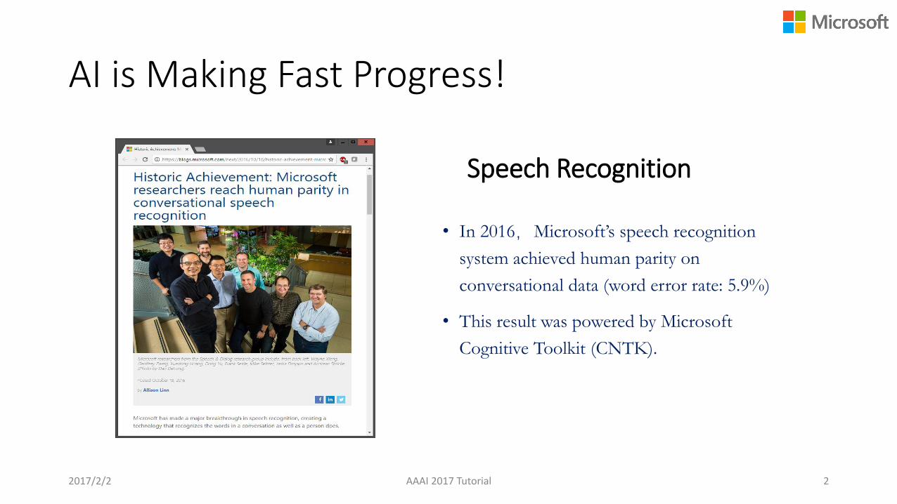
Speech Recognition
• In 2016,Microsoft’s speech recognition
system achieved human parity on
conversational data (word error rate: 5.9%)
• This result was powered by Microsoft
Cognitive Toolkit (CNTK).
2017/2/2 AAAI 2017 Tutorial 2

AI is Making Fast Progress!
2017/2/2 AAAI 2017 Tutorial 3
Image Classification Object Segmentation
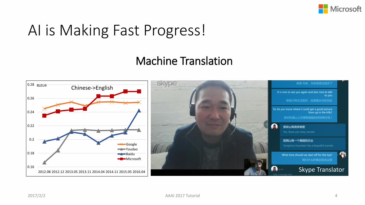
0.16
0.18
0.2
0.22
0.24
0.26
0.28
2012.08 2012.12 2013.05 2013.11 2014.04 2014.11 2015.05 2016.04
Chinese->English
Youdao
Baidu
Microsoft
BLEU4
2017/2/2 AAAI 2017 Tutorial 4
Machine Translation
AI is Making Fast Progress!
Skype Translator
AI is Making Fast Progress!
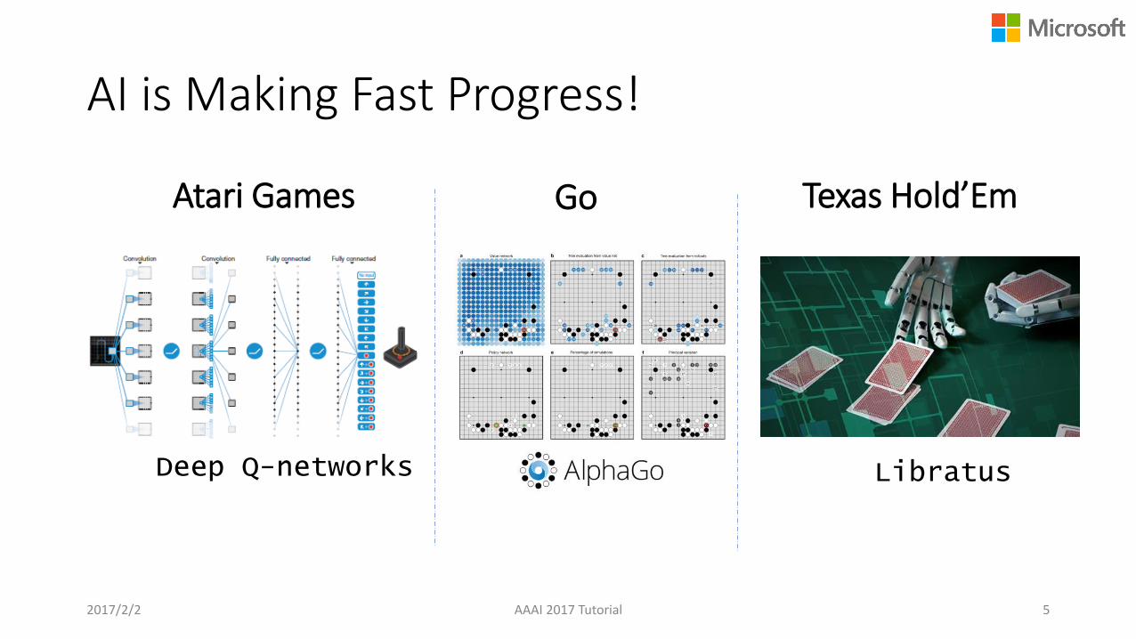
Atari Games Texas Hold’Em
Deep Q-networks
2017/2/2 AAAI 2017 Tutorial 5
Go
Libratus

The Big Trend Contributing to AI
Big Data
Big Compute
BigModel
ArtificialIntelligence
• Cloud Computing• Internet of Things• CPU/GPU/TPU/FPGA
• Statistical machine Learning (e.g., deep neural networks)
• Symbolic learning• Billions or even trillions of
parameters
• Digital Life/Work• New Form of HCI• Reinvent Productivity &
Business Process• Personal Agent
• Signals, Information & Knowledge
• Digital Representation of the World
2017/2/2 AAAI 2017 Tutorial 6

Big Data
2017/2/2 AAAI 2017 Tutorial 7
Search engine index: 1010 pages (1012 tokens)
Search engine logs: 1012 impressions and 109 clicks every year
Social networks: 109 nodes and 1012 edges
Tasks Typical training data
Image classification Millions of labeled images
Speech recognition Thousands of hours of annotated voice data
Machine translation Tens of millions of bilingual sentence pairs
Go playing Tens of millions of expert moves
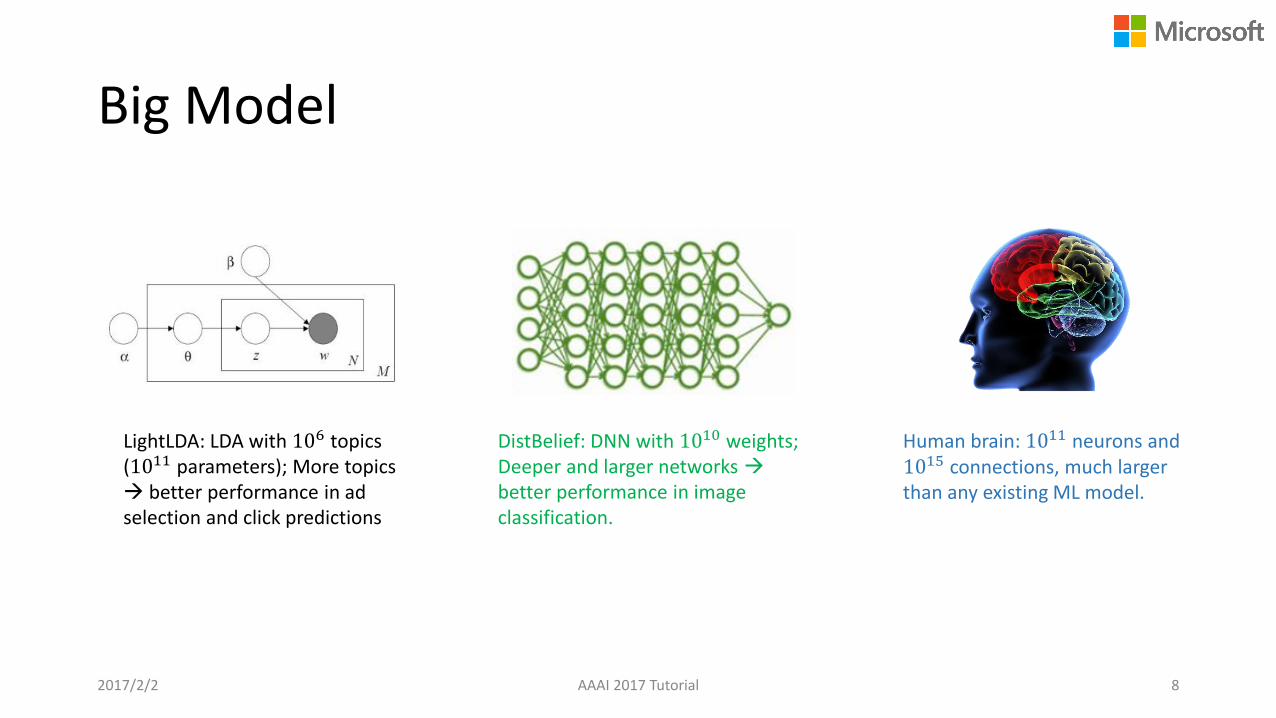
Big Model
2017/2/2 AAAI 2017 Tutorial 8
LightLDA: LDA with 106 topics (1011 parameters); More topics better performance in ad selection and click predictions
DistBelief: DNN with 1010 weights; Deeper and larger networks better performance in image classification.
Human brain: 1011 neurons and 1015 connections, much larger than any existing ML model.
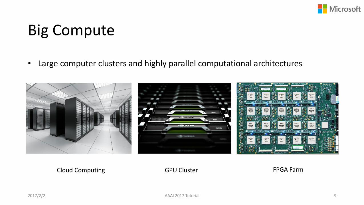
Big Compute
2017/2/2 AAAI 2017 Tutorial 9
Cloud Computing GPU Cluster FPGA Farm
• Large computer clusters and highly parallel computational architectures
2017/2/2 AAAI 2017 Tutorial 10
How to well utilize computation resourcesto speed up the training of big model over big data?
Distributed Machine Learning
2017/2/2 AAAI 2017 Tutorial 11
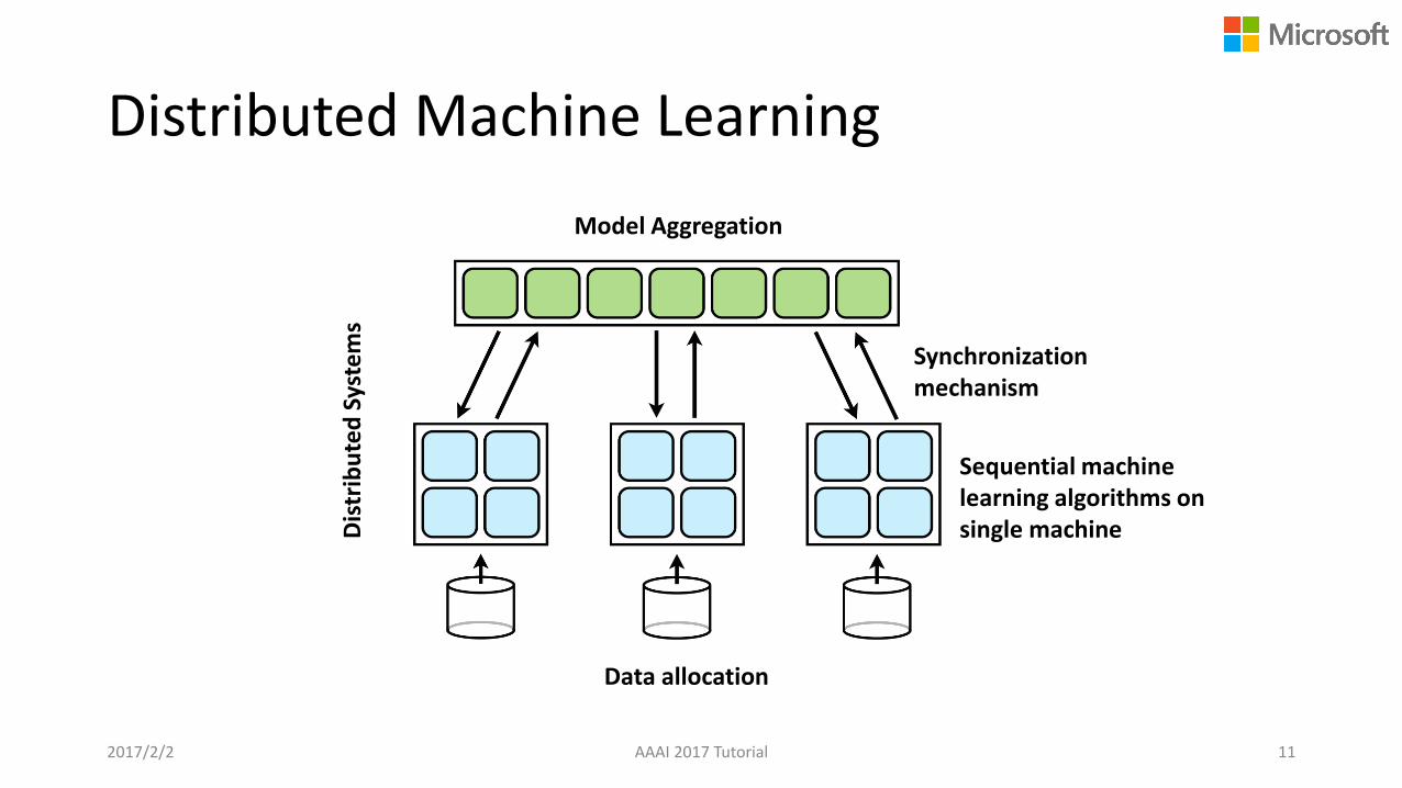
Sequential machine learning algorithms on single machine
Synchronization mechanism
Data allocation
Model Aggregation
Dis
trib
ute
d S
yste
ms

Outline of this Tutorial
2017/2/2 AAAI 2017 Tutorial 12
1. Machine Learning:Basic Framework and
Optimization Techniques
2. Distributed Machine Learning:
Foundations and Trends
3. Distributed Machine Learning:
Systems and Toolkits
• Machine learning framework• Machine learning models• Optimization algorithms:
deterministic vs. stochastic• Theoretical analysis
• Data parallelism vs. model parallelism
• Synchronous vs. asynchronous parallelization
• Data allocation• Model aggregation• Theoretical analysis
• MapReduce (Spark MLlib)• Parameter Server
(DMTK/Multiverso)• Data Flow (TensorFlow)
1. Machine Learning:Basic Framework and Optimization Techniques
2017/2/2 AAAI 2017 Tutorial 13

Machine Learning
2017/2/2 AAAI 2017 Tutorial 14
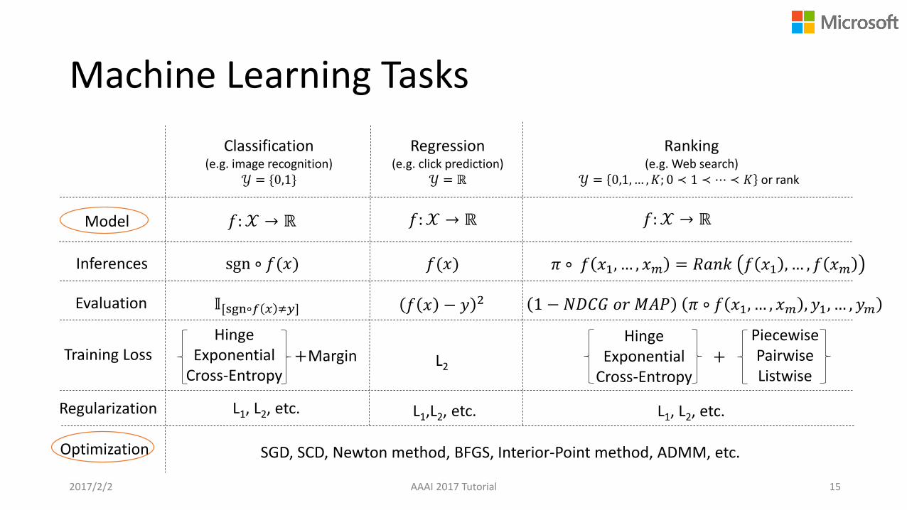
Machine Learning Tasks
2017/2/2 AAAI 2017 Tutorial 15
Classification(e.g. image recognition)
𝒴 = {0,1}
Ranking(e.g. Web search)
𝒴 = 0,1,… , 𝐾; 0 ≺ 1 ≺ ⋯ ≺ 𝐾 or rank
Regression(e.g. click prediction)
𝒴 = ℝ
𝑓:𝒳 → ℝ
Inferences
Model
sgn ∘ 𝑓(𝑥) 𝜋 ∘ 𝑓 𝑥1, … , 𝑥𝑚 = 𝑅𝑎𝑛𝑘 𝑓 𝑥1 , … , 𝑓 𝑥𝑚𝑓(𝑥)
Evaluation 𝕀[sgn∘𝑓 𝑥 ≠𝑦] 1 − 𝑁𝐷𝐶𝐺 𝑜𝑟 𝑀𝐴𝑃 𝜋 ∘ 𝑓 𝑥1, … , 𝑥𝑚 , 𝑦1, … , 𝑦𝑚𝑓 𝑥 − 𝑦 2
Training Loss
𝑓:𝒳 → ℝ𝑓:𝒳 → ℝ
HingeExponential
Cross-Entropy
HingeExponential
Cross-Entropy+
PiecewisePairwiseListwise
L2
Regularization L1, L2, etc. L1,L2, etc. L1, L2, etc.
Optimization
Margin+
SGD, SCD, Newton method, BFGS, Interior-Point method, ADMM, etc.
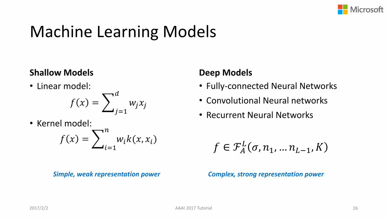
Machine Learning Models
Shallow Models
• Linear model:
𝑓 𝑥 =𝑗=1
𝑑
𝑤𝑗𝑥𝑗
• Kernel model:
𝑓 𝑥 =𝑖=1
𝑛
𝑤𝑖𝑘(𝑥, 𝑥𝑖)
Deep Models
• Fully-connected Neural Networks
• Convolutional Neural networks
• Recurrent Neural Networks
2017/2/2 AAAI 2017 Tutorial 16
𝑓 ∈ ℱ𝐴𝐿 𝜎, 𝑛1, … 𝑛𝐿−1, 𝐾
Simple, weak representation power Complex, strong representation power
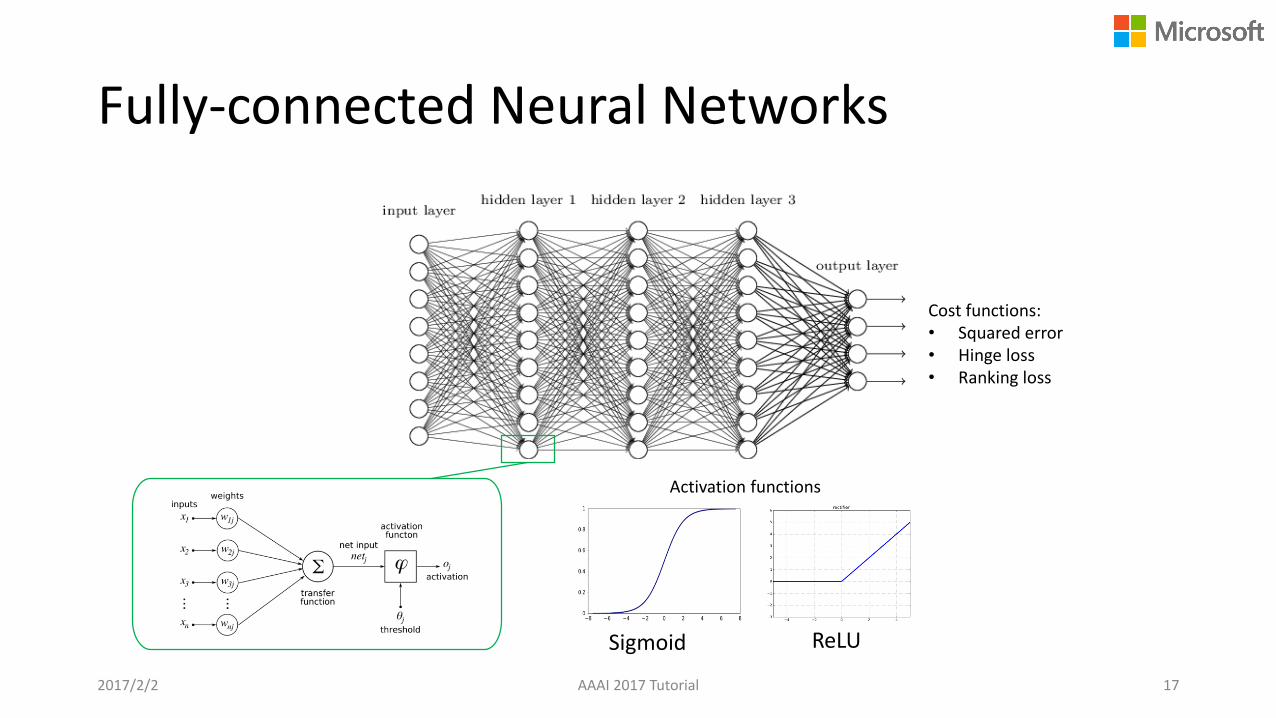
Fully-connected Neural Networks
AAAI 2017 Tutorial 17
Cost functions:• Squared error• Hinge loss• Ranking loss
Activation functions
Sigmoid ReLU
2017/2/2
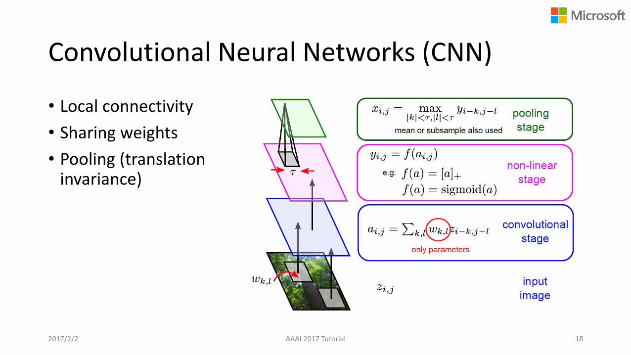
Convolutional Neural Networks (CNN)
• Local connectivity
• Sharing weights
• Pooling (translation invariance)
2017/2/2 AAAI 2017 Tutorial 18

Recurrent Neural Networks (RNN)
• Model a dynamic system driven by an external signal x• 𝐴𝑡 = 𝑓(𝑈𝑥𝑡 +𝑊𝐴𝑡−1)
• Hidden node 𝐴𝑡−1 contains information about the whole past sequence
• function 𝑓(·) maps the whole past sequence (𝑥𝑡, … , 𝑥1) to current state 𝐴𝑡
2017/2/2 AAAI 2017 Tutorial 19
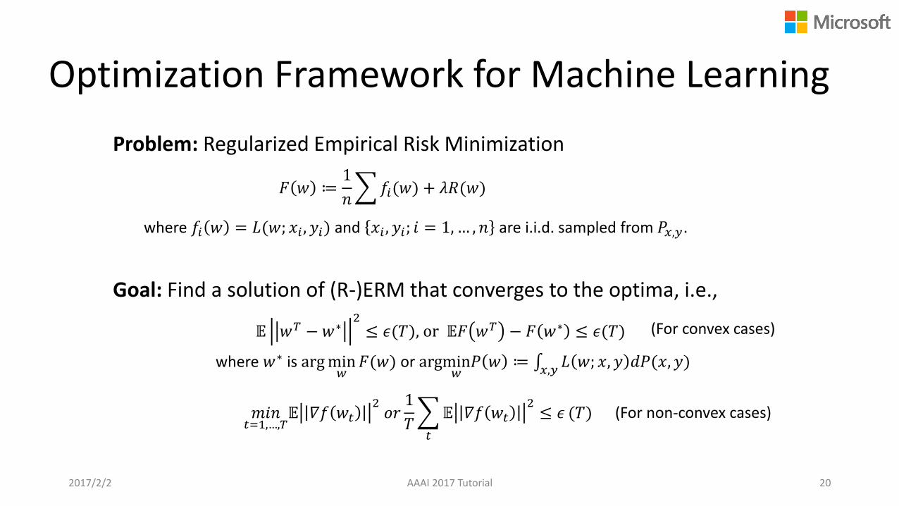
Optimization Framework for Machine Learning
Problem: Regularized Empirical Risk Minimization
𝔼 𝑤𝑇 −𝑤∗2≤ 𝜖(𝑇), or 𝔼𝐹 𝑤𝑇 − 𝐹 𝑤∗ ≤ 𝜖(𝑇)
𝐹 𝑤 ≔1
𝑛𝑓𝑖(𝑤) + 𝜆𝑅(𝑤)
Goal: Find a solution of (R-)ERM that converges to the optima, i.e.,
where 𝑓𝑖 𝑤 = 𝐿(𝑤; 𝑥𝑖 , 𝑦𝑖) and 𝑥𝑖 , 𝑦𝑖; 𝑖 = 1, … , 𝑛 are i.i.d. sampled from 𝑃𝑥,𝑦.
where 𝑤∗ is argmin𝑤
𝐹(𝑤) or argmin𝑤𝑃 𝑤 ≔ 𝑥,𝑦 𝐿 𝑤; 𝑥, 𝑦 𝑑𝑃(𝑥, 𝑦)
𝑚𝑖𝑛𝑡=1,…,𝑇
𝔼 𝛻𝑓 𝑤𝑡2𝑜𝑟
1
𝑇
𝑡
𝔼 𝛻𝑓 𝑤𝑡2≤ 𝜖 (𝑇)
2017/2/2 AAAI 2017 Tutorial 20
(For convex cases)
(For non-convex cases)
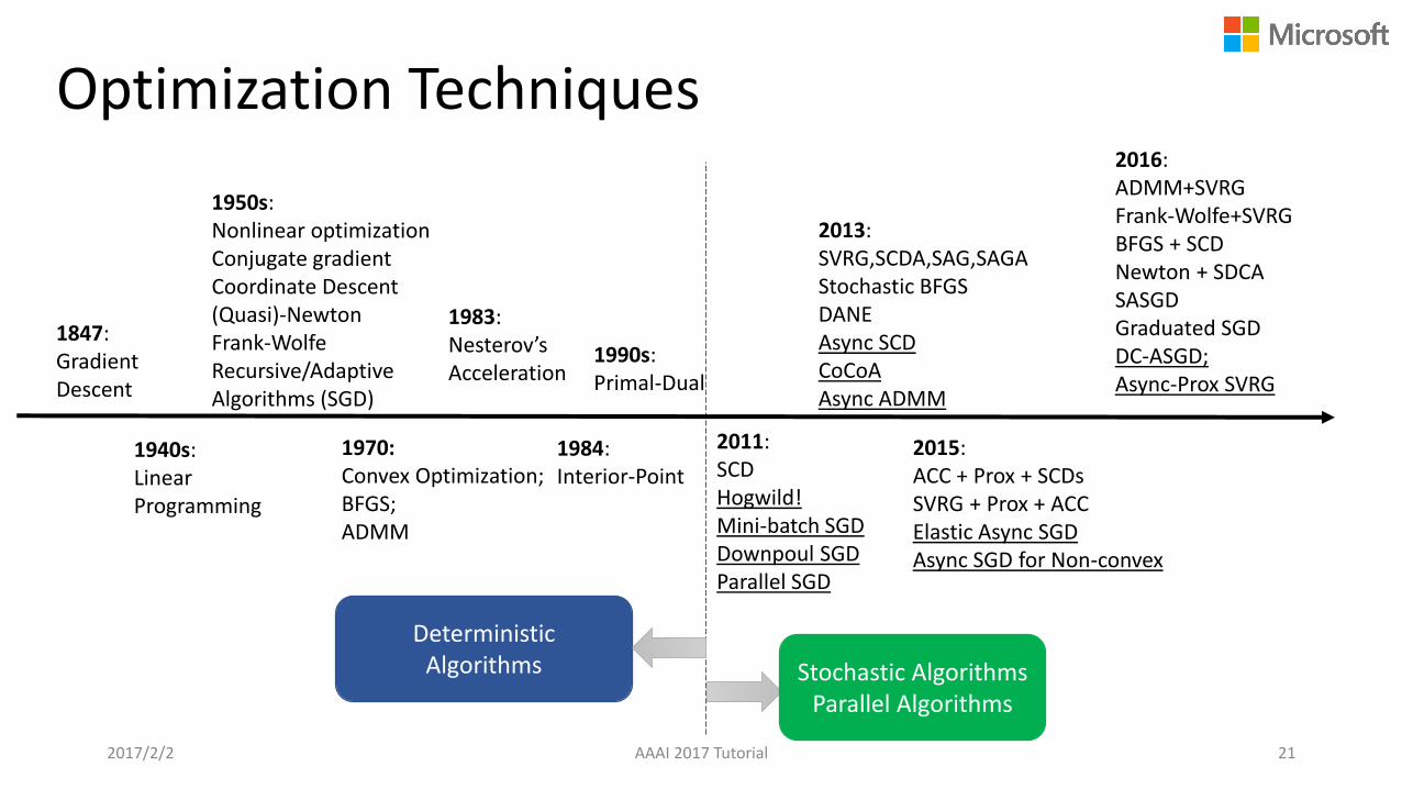
Optimization Techniques
1940s: Linear Programming
1950s: Nonlinear optimizationConjugate gradientCoordinate Descent(Quasi)-NewtonFrank-WolfeRecursive/Adaptive Algorithms (SGD)
1970: Convex Optimization;BFGS;ADMM
1984: Interior-Point
2013:SVRG,SCDA,SAG,SAGAStochastic BFGSDANEAsync SCDCoCoAAsync ADMM
2011: SCD Hogwild!Mini-batch SGDDownpoul SGDParallel SGD
1983: Nesterov’sAcceleration
2015: ACC + Prox + SCDsSVRG + Prox + ACC Elastic Async SGDAsync SGD for Non-convex
1990s: Primal-Dual
2016:ADMM+SVRGFrank-Wolfe+SVRGBFGS + SCDNewton + SDCASASGDGraduated SGDDC-ASGD; Async-Prox SVRG
DeterministicAlgorithms Stochastic Algorithms
Parallel Algorithms
1847: Gradient Descent
2017/2/2 AAAI 2017 Tutorial 21
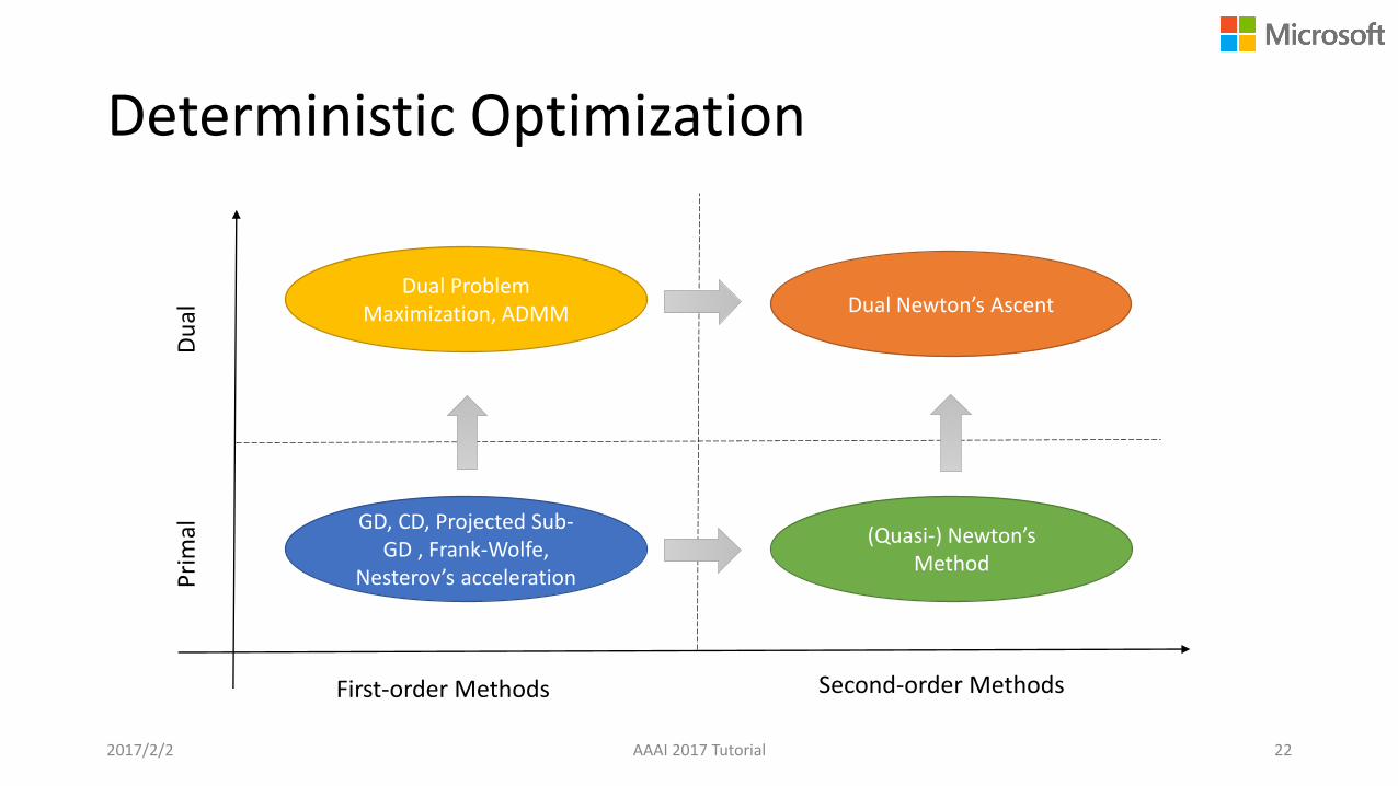
Deterministic Optimization
2017/2/2 AAAI 2017 Tutorial 22
GD, CD, Projected Sub-GD , Frank-Wolfe,
Nesterov’s acceleration
First-order Methods Second-order Methods
Pri
mal
Du
al
Dual Problem Maximization, ADMM
(Quasi-) Newton’s Method
Dual Newton’s Ascent

Stochastic Optimization
2017/2/2 AAAI 2017 Tutorial 23
First-order Methods Second-order Methods
GD, CD, Projected Sub-GD , Frank-Wolfe,
Nesterov’s accelerationPri
mal
Du
al Dual Problem Maximization,
ADMM
(Quasi-) Newton’s Method
Dual Newton’s Ascent
SGD, SCD, SVRG, SAGA,
FW+VR, ADMM+VRACC+SGD+VR, etc.
Stochastic (Quasi-) Newton’s Method
SDCA SDNA
Optimization Theory
• Conditions:• Strongly Convex, Convex, and Non-Convex
• Smoothness and Continuity
• Convergence rate:• Linear
• Super-linear
• Sub-linear
2017/2/2 AAAI 2017 Tutorial 24
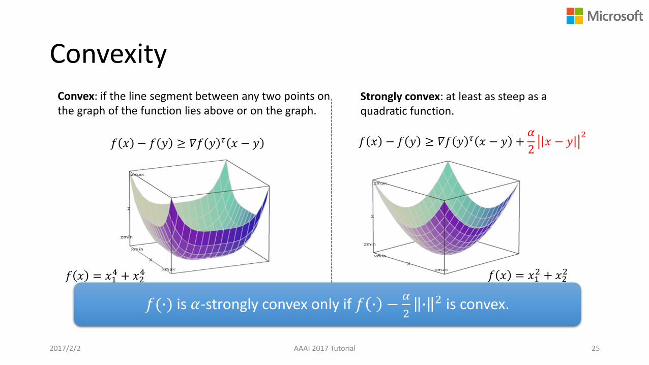
Convexity
2017/2/2 AAAI 2017 Tutorial 25
Convex Strongly-Convex
𝑓 𝑥 − 𝑓 𝑦 ≥ 𝛻𝑓 𝑦 𝜏 𝑥 − 𝑦
illustration
𝑓 𝑥 = 𝑥12 + 𝑥2
2𝑓 𝑥 = 𝑥14 + 𝑥2
4
𝑓(∙) is 𝛼-strongly convex only if 𝑓 ∙ −𝛼
2∙ 2 is convex.
Convex: if the line segment between any two points on the graph of the function lies above or on the graph.
Strongly convex: at least as steep as a quadratic function.
𝑓 𝑥 − 𝑓 𝑦 ≥ 𝛻𝑓 𝑦 𝜏 𝑥 − 𝑦 +𝛼
2𝑥 − 𝑦
2

Smoothness
2017/2/2 AAAI 2017 Tutorial 26
L-Lipschitz for non-differentiable functions
𝑓 𝑥 − 𝑓 𝑦 ≤ 𝐿 𝑥 − 𝑦
𝛽-smooth for differentiable functions
𝑓 𝑥 − 𝑓 𝑦 ≤ 𝛻𝑓 𝑥 𝜏 𝑥 − 𝑦 +𝛽
2𝑥 − 𝑦
2
𝑓 𝑥 − 𝑓 𝑦 ≥ 𝛻𝑓 𝑦 𝜏 𝑥 − 𝑦 +𝛼
2𝑥 − 𝑦
2
For 𝑥∗ ∈ argmin 𝑓(𝑥), we have𝛼
2||𝑥 − 𝑥∗||2 ≤ 𝑓 𝑥 − 𝑓 𝑥∗ ≤
𝛽
2||𝑥 − 𝑥∗||2
(𝛼 ≤ 𝛽)
𝑓(∙) is 𝛽-smooth only if 𝛻𝑓 ∙ is 𝛽-Lipschitz.
Smoothness: a small change in the input will lead to also a small change in the function output.

Convergence Rate
2017/2/2 AAAI 2017 Tutorial 27
• Equal to: linear convergence rate, e.g., 𝑂(𝑒−𝑇)
• Faster than: super-linear convergence rate, e.g., 𝑂 𝑒−𝑇2
• Slower than: sub-linear convergence rate, e.g., 𝑂1
𝑇
Does the error 𝜖(𝑇) decrease faster than 𝑒−𝑇?
1. Machine Learning:Basic Framework and Optimization Techniques
2017/2/4 AAAI 2017 Tutorial 28
Optimization Methods
•Deterministic Optimization
• Stochastic Optimization
2017/2/4 AAAI 2017 Tutorial 29

Deterministic Optimization
2017/2/4 AAAI 2017 Tutorial 30
GD, PSG, FW, Nesterov’s acceleration
First-order Methods Second-order Methods
Pri
mal
Du
al
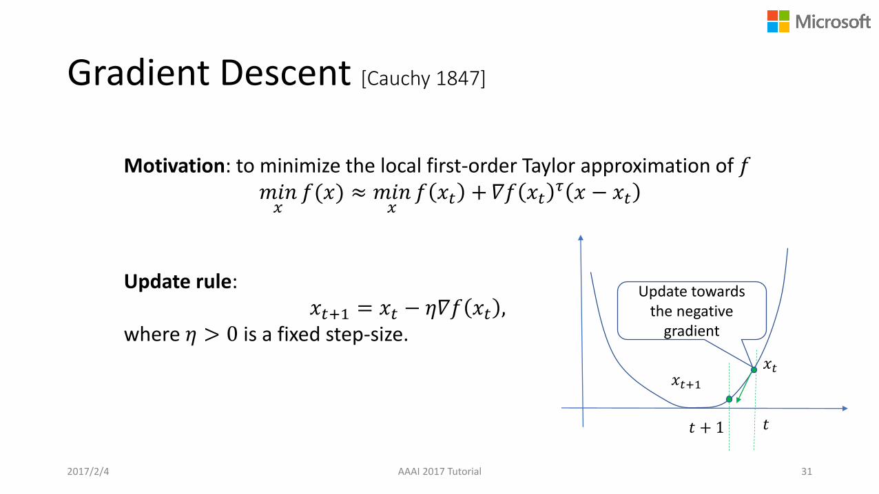
Gradient Descent [Cauchy 1847]
Motivation: to minimize the local first-order Taylor approximation of 𝑓𝑚𝑖𝑛𝑥
𝑓(𝑥) ≈ 𝑚𝑖𝑛𝑥
𝑓 𝑥𝑡 +𝛻𝑓 𝑥𝑡𝜏 𝑥 − 𝑥𝑡
Update rule:𝑥𝑡+1 = 𝑥𝑡 − 𝜂𝛻𝑓 𝑥𝑡 ,
where 𝜂 > 0 is a fixed step-size.
2017/2/4 AAAI 2017 Tutorial 31
𝑡
𝑥𝑡
Update towards the negative
gradient
𝑥𝑡+1
𝑡 + 1
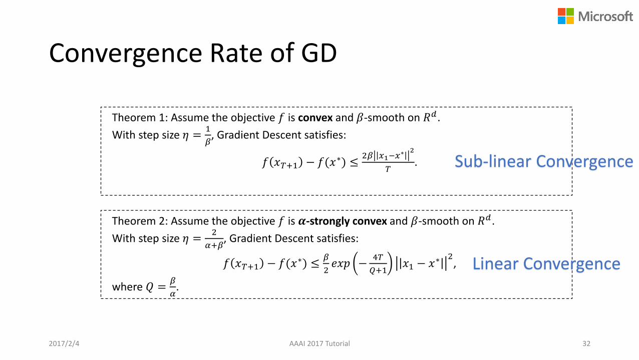
Convergence Rate of GD
2017/2/4 AAAI 2017 Tutorial 32
Theorem 2: Assume the objective 𝑓 is 𝜶-strongly convex and 𝛽-smooth on 𝑅𝑑.
With step size 𝜂 =2
𝛼+𝛽, Gradient Descent satisfies:
𝑓 𝑥𝑇+1 − 𝑓(𝑥∗) ≤𝛽
2𝑒𝑥𝑝 −
4𝑇
𝑄+1𝑥1 − 𝑥∗
2,
where 𝑄 =𝛽
𝛼.
Theorem 1: Assume the objective 𝑓 is convex and 𝛽-smooth on 𝑅𝑑.
With step size 𝜂 =1
𝛽, Gradient Descent satisfies:
𝑓 𝑥𝑇+1 − 𝑓(𝑥∗) ≤2𝛽 𝑥1−𝑥
∗ 2
𝑇.
Linear Convergence
Sub-linear Convergence
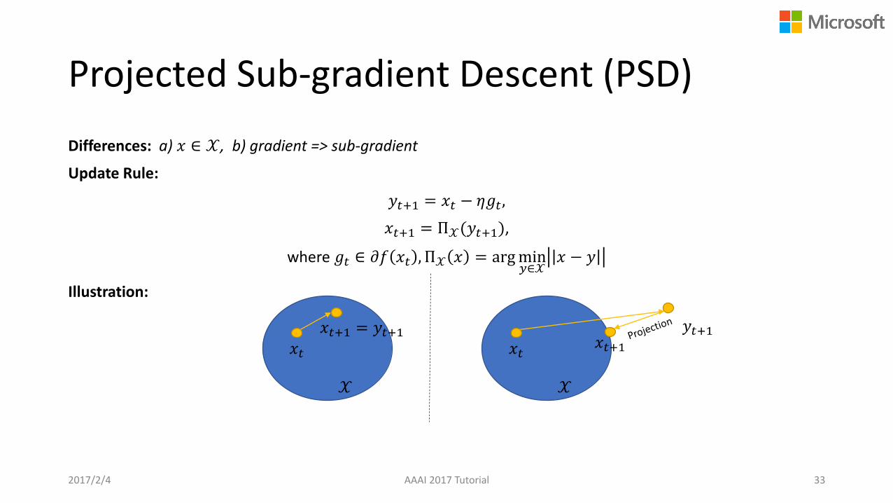
Projected Sub-gradient Descent (PSD)
Differences: a) 𝑥 ∈ 𝒳, b) gradient => sub-gradient
Update Rule:
𝑦𝑡+1 = 𝑥𝑡 − 𝜂𝑔𝑡,
𝑥𝑡+1 = Π𝒳(𝑦𝑡+1),
where 𝑔𝑡 ∈ 𝜕𝑓 𝑥𝑡 , Π𝒳 𝑥 = argmin𝑦∈𝒳
𝑥 − 𝑦
Illustration:
2017/2/4 AAAI 2017 Tutorial 33
𝑥𝑡
𝑥𝑡+1 = 𝑦𝑡+1
𝒳
𝑥𝑡
𝑦𝑡+1
𝒳
𝑥𝑡+1
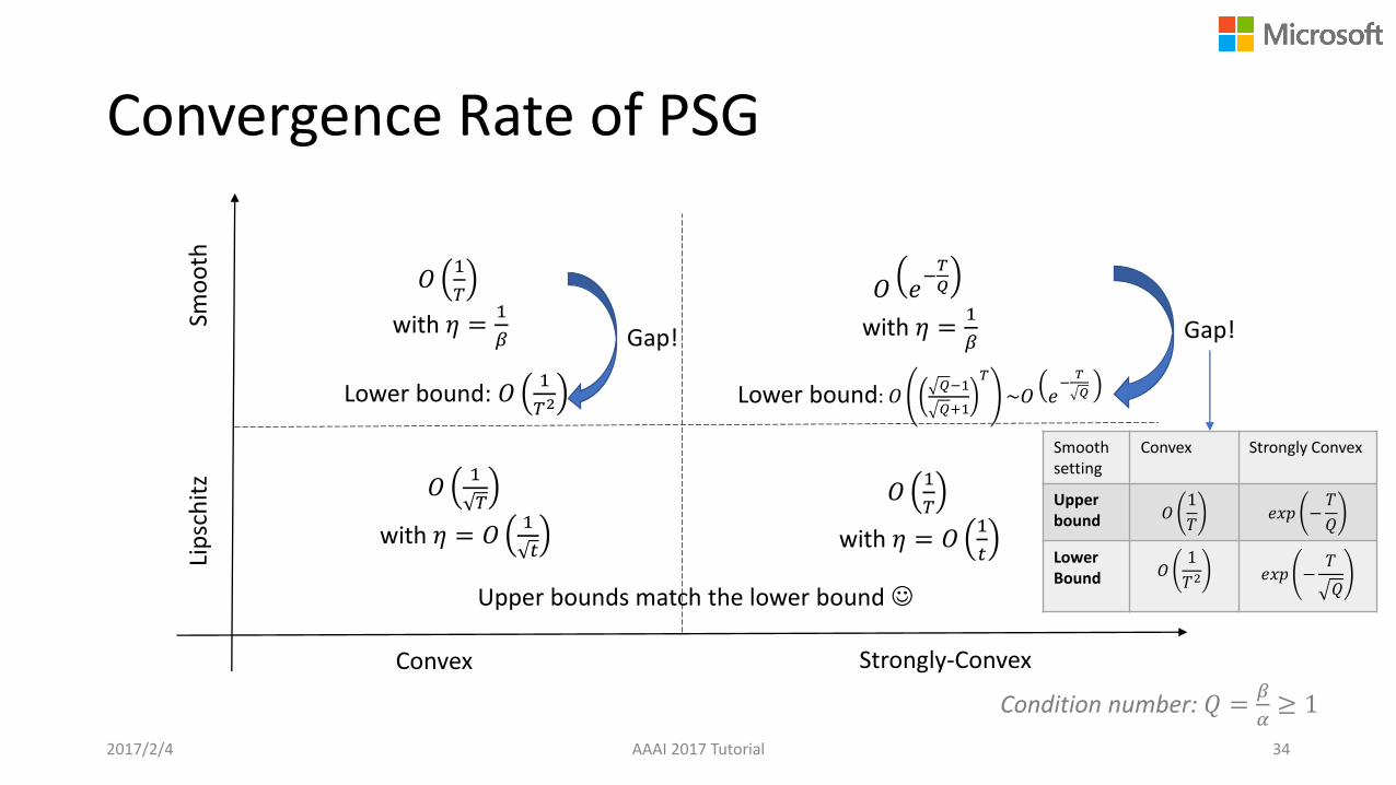
Convergence Rate of PSG
2017/2/4 AAAI 2017 Tutorial 34
Convex Strongly-Convex
Lip
sch
itz
Smo
oth
𝑂1
𝑇
with 𝜂 = 𝑂1
𝑡
𝑂1
𝑇
with 𝜂 =1
𝛽
𝑂 𝑒−𝑇
𝑄
with 𝜂 =1
𝛽
𝑂1
𝑇
with 𝜂 = 𝑂1
𝑡
Upper bounds match the lower bound
Lower bound: 𝑂1
𝑇2Lower bound: 𝑂
𝑄−1
𝑄+1
𝑇
~𝑂 𝑒−
𝑇
𝑄
Gap! Gap!
Condition number: 𝑄 =𝛽
𝛼≥ 1
Smoothsetting
Convex Strongly Convex
Upper bound 𝑂
1
𝑇𝑒𝑥𝑝 −
𝑇
𝑄
Lower Bound 𝑂
1
𝑇2 𝑒𝑥𝑝 −𝑇
𝑄
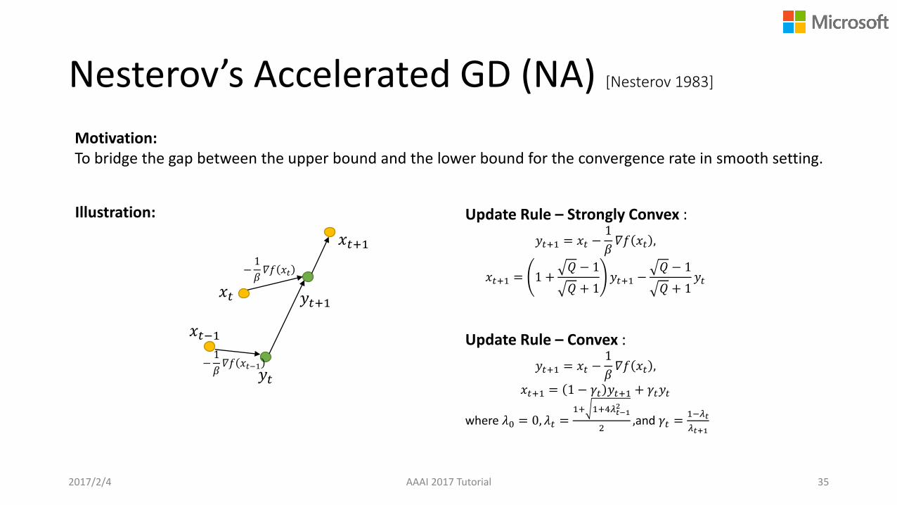
Nesterov’s Accelerated GD (NA) [Nesterov 1983]
Motivation: To bridge the gap between the upper bound and the lower bound for the convergence rate in smooth setting.
Update Rule – Strongly Convex :
𝑦𝑡+1 = 𝑥𝑡 −1
𝛽𝛻𝑓 𝑥𝑡 ,
𝑥𝑡+1 = 1 +𝑄 − 1
𝑄 + 1𝑦𝑡+1 −
𝑄 − 1
𝑄 + 1𝑦𝑡
Illustration:
Update Rule – Convex :
𝑦𝑡+1 = 𝑥𝑡 −1
𝛽𝛻𝑓 𝑥𝑡 ,
𝑥𝑡+1 = 1 − 𝛾𝑡 𝑦𝑡+1 + 𝛾𝑡𝑦𝑡
where 𝜆0 = 0, 𝜆𝑡 =1+ 1+4𝜆𝑡−1
2
2,and 𝛾𝑡 =
1−𝜆𝑡
𝜆𝑡+1
2017/2/4 AAAI 2017 Tutorial 35
𝑥𝑡 𝑦𝑡+1
−1
𝛽𝛻𝑓 𝑥𝑡
𝑦𝑡
𝑥𝑡+1
−1
𝛽𝛻𝑓 𝑥𝑡−1
𝑥𝑡−1
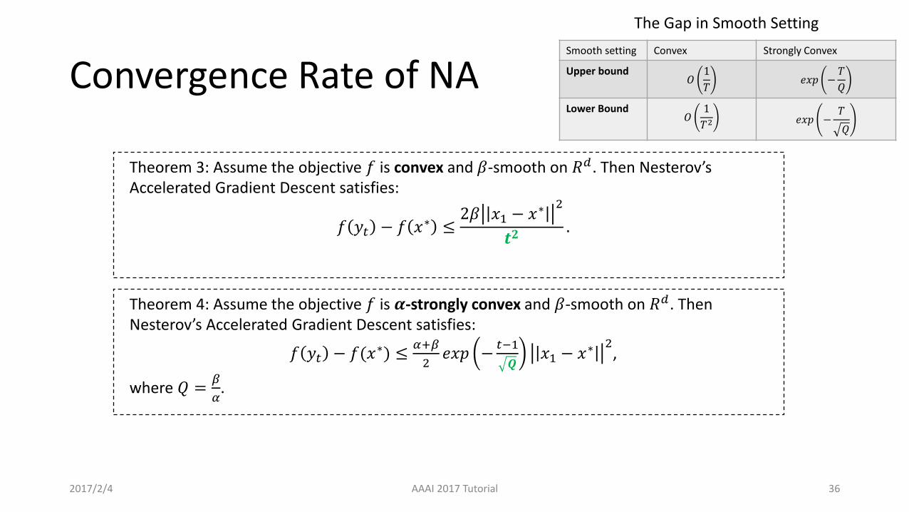
Convergence Rate of NA
2017/2/4 AAAI 2017 Tutorial 36
Smooth setting Convex Strongly Convex
Upper bound𝑂
1
𝑇𝑒𝑥𝑝 −
𝑇
𝑄
Lower Bound 𝑂
1
𝑇2 𝑒𝑥𝑝 −𝑇
𝑄
Theorem 4: Assume the objective 𝑓 is 𝜶-strongly convex and 𝛽-smooth on 𝑅𝑑. Then Nesterov’s Accelerated Gradient Descent satisfies:
𝑓 𝑦𝑡 − 𝑓(𝑥∗) ≤𝛼+𝛽
2𝑒𝑥𝑝 −
𝑡−1
𝑸𝑥1 − 𝑥∗
2,
where 𝑄 =𝛽
𝛼.
Theorem 3: Assume the objective 𝑓 is convex and 𝛽-smooth on 𝑅𝑑. Then Nesterov’sAccelerated Gradient Descent satisfies:
𝑓 𝑦𝑡 − 𝑓 𝑥∗ ≤2𝛽 𝑥1 − 𝑥∗
2
𝒕𝟐.
The Gap in Smooth Setting
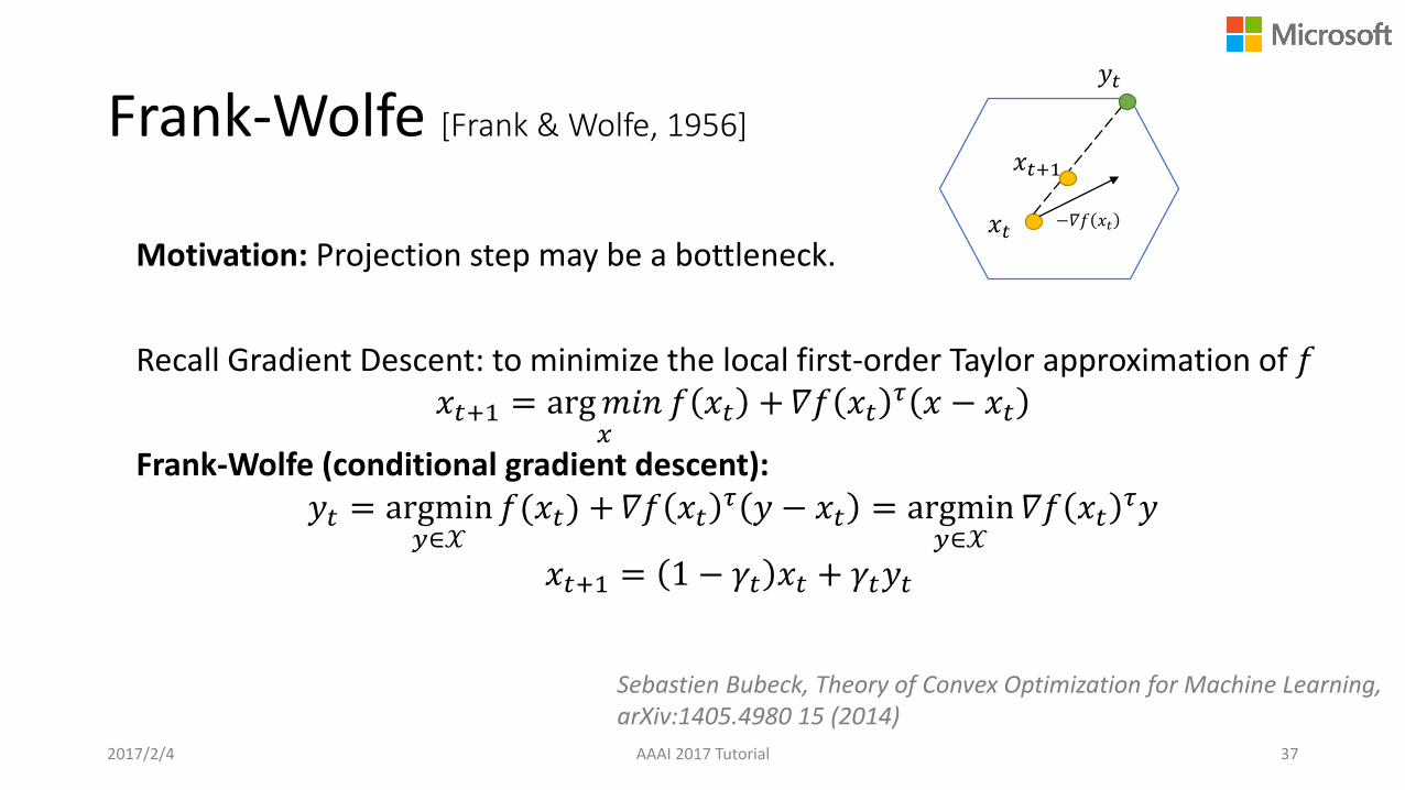
Frank-Wolfe [Frank & Wolfe, 1956]
2017/2/4 AAAI 2017 Tutorial 37
Recall Gradient Descent: to minimize the local first-order Taylor approximation of 𝑓𝑥𝑡+1 = arg𝑚𝑖𝑛
𝑥𝑓 𝑥𝑡 +𝛻𝑓 𝑥𝑡
𝜏 𝑥 − 𝑥𝑡
Frank-Wolfe (conditional gradient descent): 𝑦𝑡 = argmin
𝑦∈𝒳𝑓(𝑥𝑡) +𝛻𝑓 𝑥𝑡
𝜏 𝑦 − 𝑥𝑡 = argmin𝑦∈𝒳
𝛻𝑓 𝑥𝑡𝜏𝑦
𝑥𝑡+1 = 1 − 𝛾𝑡 𝑥𝑡 + 𝛾𝑡𝑦𝑡
Motivation: Projection step may be a bottleneck. 𝑥𝑡 −𝛻𝑓 𝑥𝑡
𝑦𝑡
𝑥𝑡+1
Sebastien Bubeck, Theory of Convex Optimization for Machine Learning, arXiv:1405.4980 15 (2014)
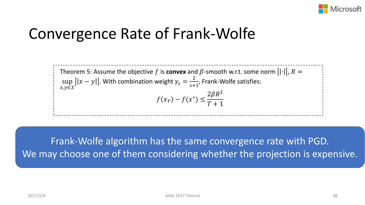
Convergence Rate of Frank-Wolfe
2017/2/4 AAAI 2017 Tutorial 38
Theorem 5: Assume the objective 𝑓 is convex and 𝛽-smooth w.r.t. some norm ⋅ , 𝑅 =
sup𝑥,𝑦∈𝒳
𝑥 − 𝑦 . With combination weight 𝛾𝑠 =2
𝑠+1, Frank-Wolfe satisfies:
𝑓 𝑥𝑇 − 𝑓(𝑥∗) ≤2𝛽𝑅2
𝑇 + 1
Frank-Wolfe algorithm has the same convergence rate with PGD.We may choose one of them considering whether the projection is expensive.
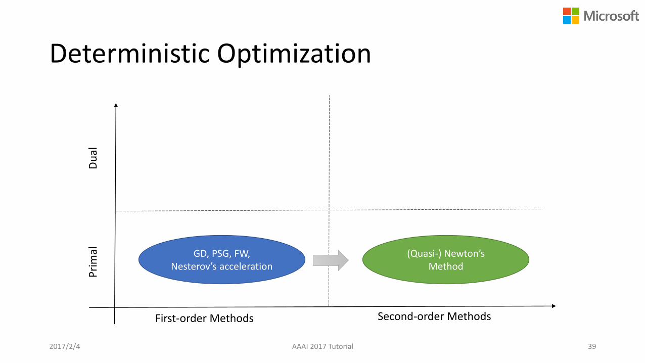
Deterministic Optimization
2017/2/4 AAAI 2017 Tutorial 39
First-order Methods Second-order Methods
GD, PSG, FW, Nesterov’s acceleration
Pri
mal
Du
al
(Quasi-) Newton’s Method

Newton’s Methods
Motivation: To minimize the local second-order Taylor approximation of 𝑓:
𝑚𝑖𝑛𝑥
𝑓(𝑥) ≈ 𝑚𝑖𝑛𝑥
𝑓 𝑥𝑡 +𝛻𝑓 𝑥𝑡𝜏 𝑥 − 𝑥𝑡 +
1
2𝑥 − 𝑥𝑡
𝜏𝛻2𝑓 𝑥𝑡 𝑥 − 𝑥𝑡 + 𝑜 𝑥 − 𝑥𝑡2.
Update Rule: suppose 𝛻2𝑓(𝑥t) is positive definite,
𝑥𝑡+1 = 𝑥𝑡 − 𝛻2𝑓 𝑥𝑡−1𝛻𝑓(𝑥𝑡)
2017/2/4 AAAI 2017 Tutorial 40
A more dedicate step size, comparing to GD.
𝑡
𝑥𝑡𝑥𝑡+1
𝑡 + 1
𝑓(𝑥)
the minimizer of the second-order approximation of 𝑓
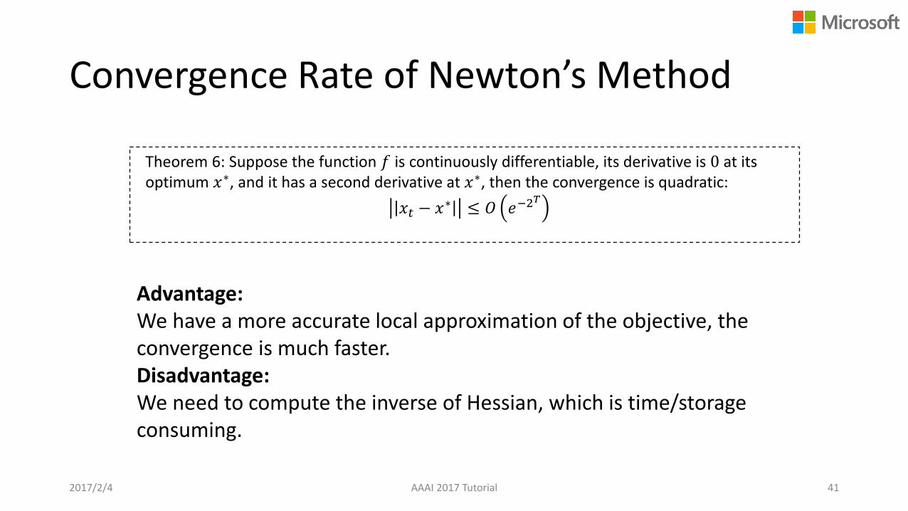
Convergence Rate of Newton’s Method
2017/2/4 AAAI 2017 Tutorial 41
Theorem 6: Suppose the function 𝑓 is continuously differentiable, its derivative is 0 at its optimum 𝑥∗, and it has a second derivative at 𝑥∗, then the convergence is quadratic:
𝑥𝑡 − 𝑥∗ ≤ 𝑂 𝑒−2𝑇
Advantage: We have a more accurate local approximation of the objective, the convergence is much faster.Disadvantage: We need to compute the inverse of Hessian, which is time/storage consuming.

Quasi Newton’s Methods
Denote 𝐵𝑡 = 𝛻2𝑓 𝑥𝑡 , 𝐻𝑡 = 𝛻2𝑓 𝑥𝑡−1
Main Idea: The inverse of Hessian is approximated by rank one updates of the gradient evaluations, under the Quasi-Newton’s condition.
𝑓(𝑥) ≈ 𝑓 𝑥𝑡 + 𝛻𝑓 𝑥𝑡𝜏 𝑥 − 𝑥𝑡 +
1
2𝑥 − 𝑥𝑡
𝜏𝐵𝑡 𝑥 − 𝑥𝑡
𝛻𝑓 𝑥 ≈ 𝛻𝑓 𝑥𝑡 + 𝐵𝑡 𝑥 − 𝑥𝑡 //Calculate gradients for both sides
Bt−1𝑦𝑡 ≈ 𝑠𝑡 // Let 𝑥 = 𝑥𝑡+1,
where 𝑦𝑡 = 𝛻𝑓 𝑥𝑡+1 − 𝛻𝑓(𝑥𝑡), 𝑠𝑡 = 𝑥𝑡+1 − 𝑥𝑡
𝐵𝑡+1 = 𝐵𝑡 + 𝑎𝑎𝜏 + 𝑏𝑏𝜏
2017/2/4 AAAI 2017 Tutorial 42
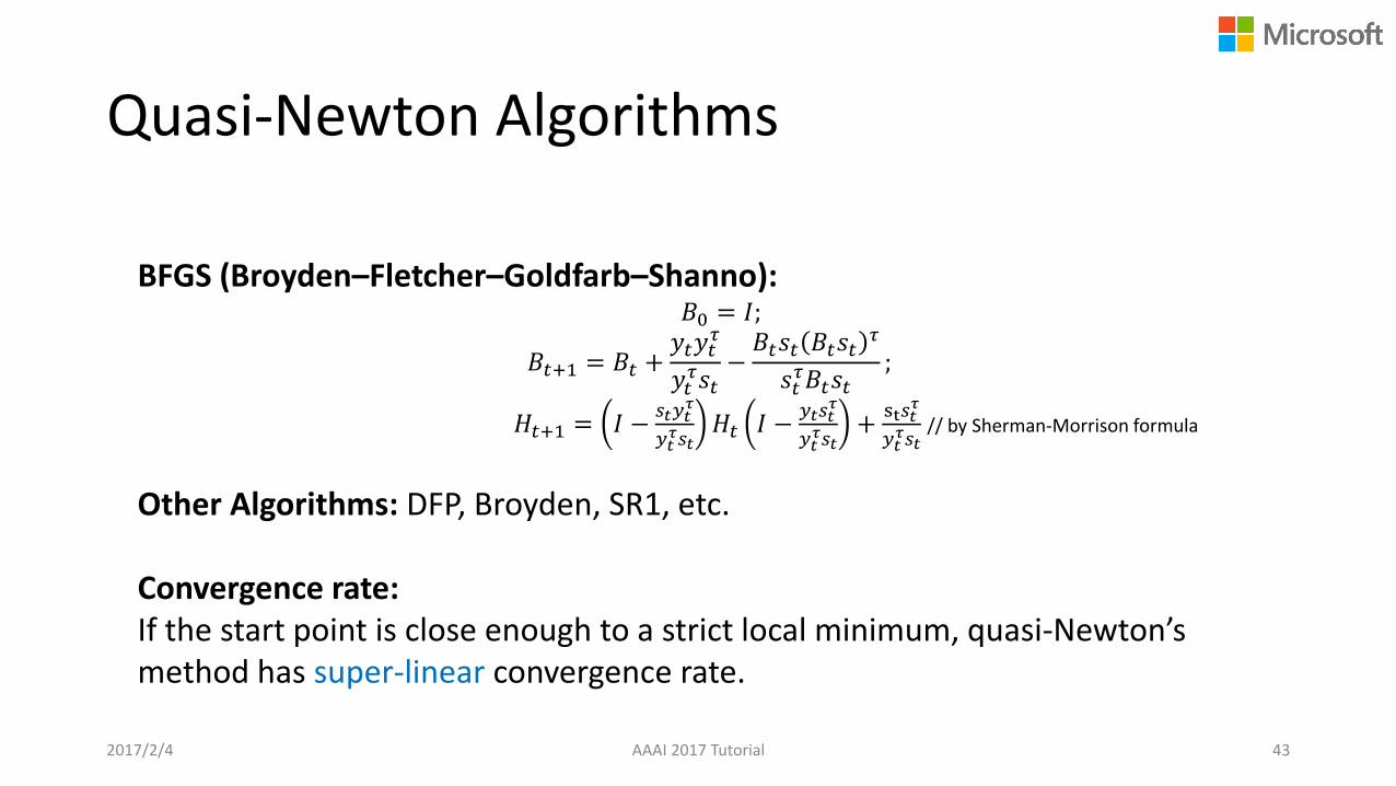
Quasi-Newton Algorithms
BFGS (Broyden–Fletcher–Goldfarb–Shanno):𝐵0 = 𝐼;
𝐵𝑡+1 = 𝐵𝑡 +𝑦𝑡𝑦𝑡
𝜏
𝑦𝑡𝜏𝑠𝑡
−𝐵𝑡𝑠𝑡 𝐵𝑡𝑠𝑡
𝜏
𝑠𝑡𝜏𝐵𝑡𝑠𝑡
;
𝐻𝑡+1 = 𝐼 −𝑠𝑡𝑦𝑡
𝜏
𝑦𝑡𝜏𝑠𝑡
𝐻𝑡 𝐼 −𝑦𝑡𝑠𝑡
𝜏
𝑦𝑡𝜏𝑠𝑡
+st𝑠𝑡
𝜏
𝑦𝑡𝜏𝑠𝑡
// by Sherman-Morrison formula
Other Algorithms: DFP, Broyden, SR1, etc.
Convergence rate:If the start point is close enough to a strict local minimum, quasi-Newton’s method has super-linear convergence rate.
2017/2/4 AAAI 2017 Tutorial 43

Summary – Deterministic Algorithms
Algorithms Convergence rates
GD𝑂 exp −
𝑡
𝑄
ACC-GD𝑂 exp −
𝑡
𝑄
PGD𝑂 exp −
𝑡
𝑄
Frank-Wolfe𝑂 exp −
𝑡
𝑄
Newton 𝑂 exp −𝑒2𝑡
Quasi-Newton -BFGS 𝑂 exp −𝑒2𝑡
Strongly convex + smooth
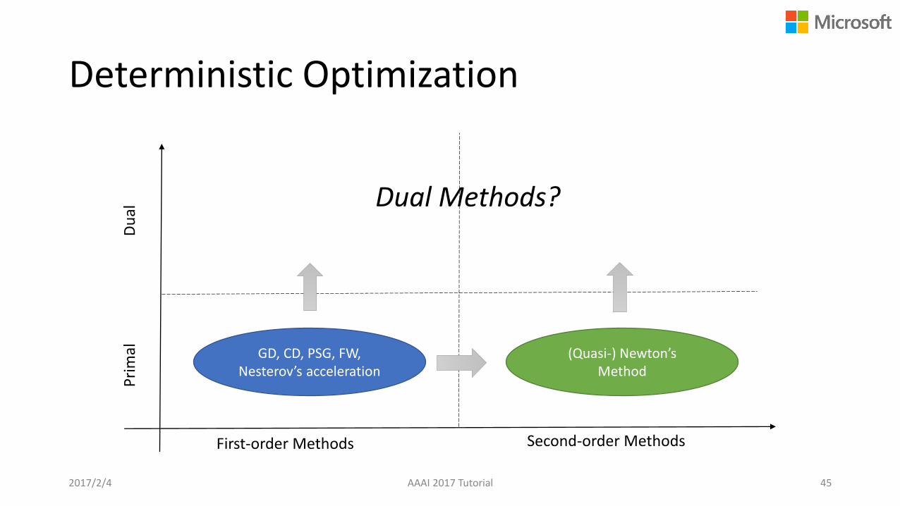
Deterministic Optimization
2017/2/4 AAAI 2017 Tutorial 45
First-order Methods Second-order Methods
GD, CD, PSG, FW, Nesterov’s acceleration
Pri
mal
Du
al
(Quasi-) Newton’s Method
Dual Methods?

Primal-Dual: Lagrangian
Primal Problem: min𝑥
𝑓0(𝑥)
𝑠. 𝑡. 𝑓𝑖 𝑥 ≤ 0, 𝑖 = 1,… ,𝑚ℎ𝑖 𝑥 = 0, 𝑗 = 1,… , 𝑝
Optimal value: 𝑝∗
Linear approximation to the indicator function The Lagrangian:
𝐿 𝑥, 𝜆, 𝜈 ≜ 𝑓0 𝑥 +
𝑖=1
𝑚
𝜆𝑖𝑓𝑖 𝑥 +
𝑗=1
𝑝
𝜈𝑖ℎ𝑖 𝑥
where 𝜆𝑖 ≥ 0, 𝜈𝑗 ∈ 𝑅.
2017/2/4 AAAI 2017 Tutorial 46
A problem with hard constraints => A series of problems with soft constraints

ADMM
2017/2/4 AAAI 2017 Tutorial 47
Separable objective with a constraint:𝑚𝑖𝑛𝑥,𝑧
𝑓 𝑥 + 𝑔 𝑧
𝑠. 𝑡. 𝐴𝑥 + 𝐵𝑧 = 𝑐
Augmented Lagrangian: 𝜌 > 0
𝐿𝜌 𝑥, 𝑦, 𝑧 = 𝑓 𝑥 + 𝑔 𝑧 + 𝑦𝑇 𝐴𝑥 + 𝐵𝑧 − 𝑐 +𝜌
2𝐴𝑥 + 𝐵𝑧 − 𝑐
2
ADMM’s Partial Updates: 𝑥𝑡+1 = 𝑎𝑟𝑔𝑚𝑖𝑛𝑥𝐿𝜌(𝑥, 𝑧
𝑡 , 𝑦𝑡) -------𝑥 minimization
𝑧𝑡+1 = 𝑎𝑟𝑔𝑚𝑖𝑛𝑧𝐿𝜌(𝑥𝑡+1, 𝑧, 𝑦𝑡) -------𝑦 minimization
𝑦𝑡+1 = 𝑦𝑡 + 𝜌(𝐴𝑥𝑡+1 + 𝐵𝑧𝑡+1 − 𝑐) -------dual ascent update
For example, in DML:
𝑚𝑖𝑛𝑥𝑘,𝑧
σ𝑘=1𝐾 𝑓𝑘 𝑥𝑘 , 𝐷𝑘
s.t. 𝑥𝑘 = 𝑧, ∀𝑘 = 1,… , 𝐾.
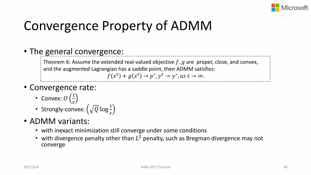
Convergence Property of ADMM
• The general convergence:
• Convergence rate:• Convex: 𝑂
1
𝜖
• Strongly-convex: 𝑄 log1
𝜖
• ADMM variants:• with inexact minimization still converge under some conditions• with divergence penalty other than 𝐿2 penalty, such as Bregman divergence may not
converge
2017/2/4 AAAI 2017 Tutorial 48
Theorem 6: Assume the extended real-valued objective 𝑓, 𝑔 are proper, close, and convex, and the augmented Lagrangian has a saddle point, then ADMM satisfies:
𝑓 𝑥𝑡 + 𝑔 𝑧𝑡 → 𝑝∗, 𝑦𝑡 → 𝑦∗, 𝑎𝑠 𝑡 → ∞.
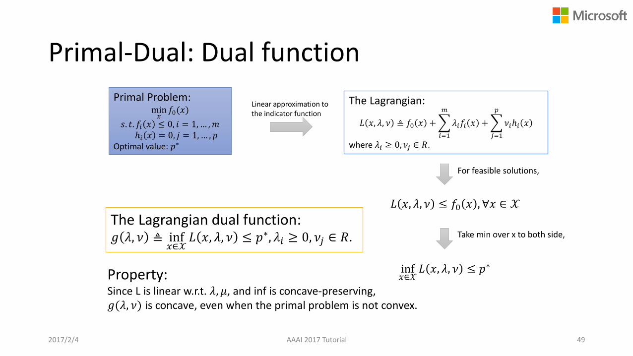
Primal-Dual: Dual function
Primal Problem: min𝑥
𝑓0(𝑥)
𝑠. 𝑡. 𝑓𝑖 𝑥 ≤ 0, 𝑖 = 1,… ,𝑚ℎ𝑖 𝑥 = 0, 𝑗 = 1,… , 𝑝
Optimal value: 𝑝∗
Linear approximation to the indicator function
The Lagrangian:
𝐿 𝑥, 𝜆, 𝜈 ≜ 𝑓0 𝑥 +
𝑖=1
𝑚
𝜆𝑖𝑓𝑖 𝑥 +
𝑗=1
𝑝
𝜈𝑖ℎ𝑖 𝑥
where 𝜆𝑖 ≥ 0, 𝜈𝑗 ∈ 𝑅.
For feasible solutions,
𝐿 𝑥, 𝜆, 𝜈 ≤ 𝑓0 𝑥 , ∀𝑥 ∈ 𝒳
The Lagrangian dual function:𝑔 𝜆, 𝜈 ≜ inf
𝑥∈𝒳𝐿 𝑥, 𝜆, 𝜈 ≤ 𝑝∗, 𝜆𝑖 ≥ 0, 𝜈𝑗 ∈ 𝑅.
2017/2/4 AAAI 2017 Tutorial 49
Take min over x to both side,
inf𝑥∈𝒳
𝐿 𝑥, 𝜆, 𝜈 ≤ 𝑝∗Property: Since L is linear w.r.t. 𝜆, 𝜇, and inf is concave-preserving,𝑔(𝜆, 𝜈) is concave, even when the primal problem is not convex.

Primal-Dual: Dual Problem
Primal Problem: min𝑥
𝑓0(𝑥)
𝑠. 𝑡. 𝑓𝑖 𝑥 ≤ 0, 𝑖 = 1,… ,𝑚ℎ𝑖 𝑥 = 0, 𝑗 = 1,… , 𝑝
Optimal value: 𝑝∗
Linear approximation to the indicator function
The Lagrangian:
𝐿 𝑥, 𝜆, 𝜈 ≜ 𝑓0 𝑥 +
𝑖=1
𝑚
𝜆𝑖𝑓𝑖 𝑥 +
𝑗=1
𝑝
𝜈𝑖ℎ𝑖 𝑥
where 𝜆𝑖 ≥ 0, 𝜈𝑗 ∈ 𝑅.
The Lagrangian dual function:𝑔 𝜆, 𝜈 ≜ inf
𝑥∈𝒳𝐿 𝑥, 𝜆, 𝜈 ≤ 𝑝∗, 𝜆𝑖 ≥ 0, 𝜈𝑗 ∈ 𝑅.
The best lower bound of 𝑝∗?
Dual Problem: max𝜆,𝜈
𝑔 𝜆, 𝜈
𝑠. 𝑡. 𝜆𝑖 ≥ 0, 𝑖 = 1,… ,𝑚The dual problem is convex.Optimal value: 𝑑∗
2017/2/4 AAAI 2017 Tutorial 50

Primal-Dual: Duality
Primal Problem: min𝑥
𝑓0(𝑥)
𝑠. 𝑡. 𝑓𝑖 𝑥 ≤ 0, 𝑖 = 1,… ,𝑚ℎ𝑖 𝑥 = 0, 𝑗 = 1,… , 𝑝
Optimal value: 𝑝∗
The Lagrangian:
𝐿 𝑥, 𝜆, 𝜈 ≜ 𝑓0 𝑥 +
𝑖=1
𝑚
𝜆𝑖𝑓𝑖 𝑥 +
𝑗=1
𝑝
𝜈𝑖ℎ𝑖 𝑥
where 𝜆𝑖 ≥ 0, 𝜈𝑗 ∈ 𝑅.
The Lagrangian dual function:𝑔 𝜆, 𝜈 ≜ inf
𝑥∈𝒳𝐿 𝑥, 𝜆, 𝜈 ≤ 𝑝∗, 𝜆𝑖 ≥ 0, 𝜈𝑗 ∈ 𝑅.
Property: concave, even when the primal problem is not convex.
Dual Problem: max𝜆,𝜈
𝑔 𝜆, 𝜈
𝑠. 𝑡. 𝜆𝑖 ≥ 0, 𝑖 = 1,… ,𝑚The dual problem is concave.Optimal value: 𝑑∗
Weak duality always holds: 𝑑∗ ≤ 𝑝∗.When will strong duality 𝑑∗ = 𝑝∗hold? E.g., Slater’s condition. An necessary condition for differentiable problem: KKT
Dual Optimal:(𝜆∗, 𝜈∗)
min𝑥
𝐿 𝑥, 𝜆, 𝜈
If feasible
2017/2/4 AAAI 2017 Tutorial 51
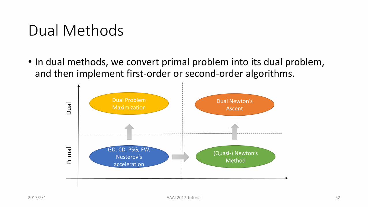
Dual Methods
• In dual methods, we convert primal problem into its dual problem, and then implement first-order or second-order algorithms.
2017/2/4 AAAI 2017 Tutorial 52
GD, CD, PSG, FW, Nesterov’s
accelerationPri
mal
Du
al
Dual Problem Maximization
(Quasi-) Newton’s Method
Dual Newton’s Ascent
Optimization Methods
•Deterministic Optimization
• Stochastic Optimization
2017/2/4 AAAI 2017 Tutorial 53
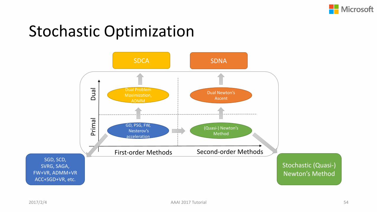
Stochastic Optimization
2017/2/4 AAAI 2017 Tutorial 54
First-order Methods Second-order Methods
GD, PSG, FW, Nesterov’s
accelerationPri
mal
Du
al Dual Problem Maximization,
ADMM
(Quasi-) Newton’s Method
Dual Newton’s Ascent
SGD, SCD, SVRG, SAGA,
FW+VR, ADMM+VRACC+SGD+VR, etc.
Stochastic (Quasi-) Newton’s Method
SDCA SDNA
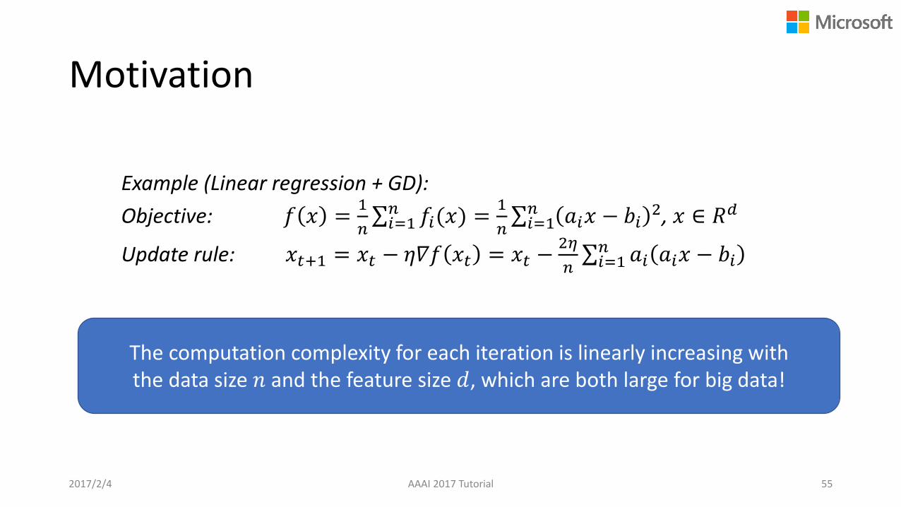
Motivation
Example (Linear regression + GD):
Objective: 𝑓 𝑥 =1
𝑛σ𝑖=1𝑛 𝑓𝑖(𝑥) =
1
𝑛σ𝑖=1𝑛 𝑎𝑖𝑥 − 𝑏𝑖
2, 𝑥 ∈ 𝑅𝑑
Update rule: 𝑥𝑡+1 = 𝑥𝑡 − 𝜂𝛻𝑓 𝑥𝑡 = 𝑥𝑡 −2𝜂
𝑛σ𝑖=1𝑛 𝑎𝑖 𝑎𝑖𝑥 − 𝑏𝑖
The computation complexity for each iteration is linearly increasing with the data size 𝑛 and the feature size 𝑑, which are both large for big data!
2017/2/4 AAAI 2017 Tutorial 55
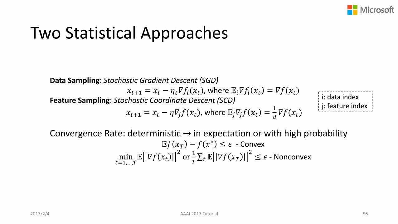
Two Statistical Approaches
i: data indexj: feature index
Convergence Rate: deterministic → in expectation or with high probability𝔼𝑓 𝑥𝑇 − 𝑓 𝑥∗ ≤ 𝜖 - Convex
min𝑡=1,…,𝑇
𝔼 𝛻𝑓 𝑥𝑡2or
1
𝑇σ𝑡𝔼 𝛻𝑓 𝑥𝑇
2≤ 𝜖 - Nonconvex
Data Sampling: Stochastic Gradient Descent (SGD) 𝑥𝑡+1 = 𝑥𝑡 − 𝜂𝑡𝛻𝑓𝑖(𝑥𝑡), where 𝔼𝑖𝛻𝑓𝑖 𝑥𝑡 = 𝛻𝑓(𝑥𝑡)
Feature Sampling: Stochastic Coordinate Descent (SCD)
𝑥𝑡+1 = 𝑥𝑡 − 𝜂𝛻𝑗𝑓(𝑥𝑡), where 𝔼𝑗𝛻𝑗𝑓 𝑥𝑡 =1
𝑑𝛻𝑓(𝑥𝑡)
2017/2/4 AAAI 2017 Tutorial 56
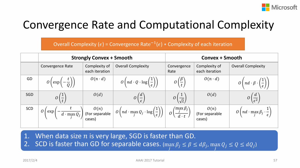
Convergence Rate and Computational Complexity
Overall Complexity (𝜖) = Convergence Rate−1(𝜖) ∗ Complexity of each iteration
1. When data size 𝑛 is very large, SGD is faster than GD.2. SCD is faster than GD for separable cases. (max
𝑗𝛽𝑗 ≤ 𝛽 ≤ 𝑑𝛽𝑗, max
𝑗𝑄𝑗 ≤ 𝑄 ≤ 𝑑𝑄𝑗)
Strongly Convex + Smooth Convex + Smooth
Convergence Rate Complexity of each iteration
Overall Complexity Convergence Rate
Complexity of each iteration
Overall Complexity
GD𝑂 exp −
𝑡
𝑄
𝑂(𝑛 ⋅ 𝑑)𝑂 𝑛𝑑 ⋅ 𝑄 ⋅ log
1
𝜖𝑂
𝛽
𝑡
𝑂(𝑛 ⋅ 𝑑)𝑂 𝑛𝑑 ⋅ 𝛽 ⋅
1
𝜖
SGD𝑂
1
𝑡
𝑂(𝑑)𝑂
𝑑
𝜖𝑂
1
𝑡
𝑂(𝑑)𝑂
𝑑
𝜖2
SCD𝑂 exp −
𝑡
𝑑 ⋅ max𝑗
𝑄𝑗
𝑂(𝑛)(For separable cases)
𝑂 𝑛𝑑 ⋅ max𝑗
𝑄𝑗 ⋅ log1
𝜖 𝑂max𝑗
𝛽𝑗
𝑑 ⋅ 𝑡
𝑂(𝑛)(For separable cases)
𝑂 𝑛𝑑 ⋅ max𝑗
𝛽𝑗 ⋅1
𝜖
2017/2/4 AAAI 2017 Tutorial 57
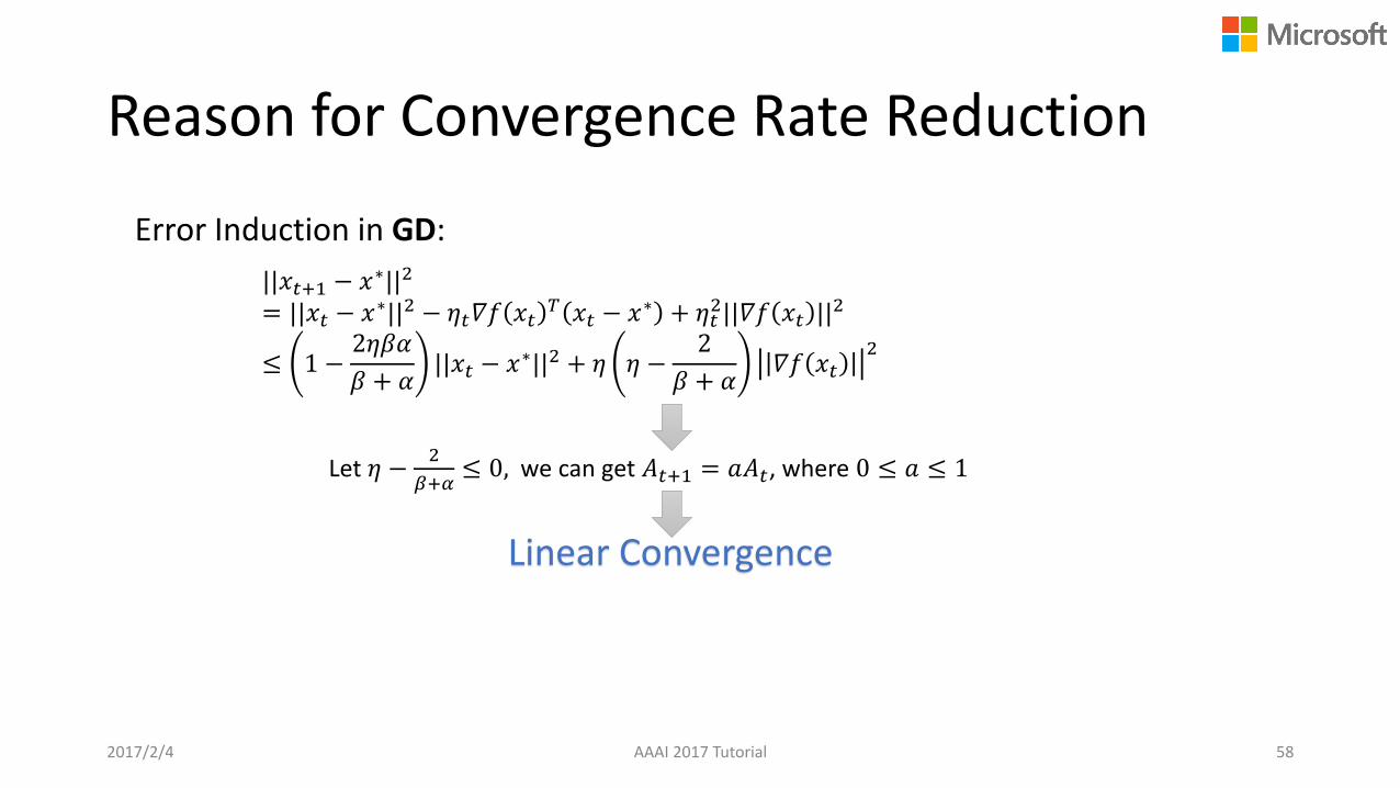
Reason for Convergence Rate Reduction
Error Induction in GD:
||𝑥𝑡+1 − 𝑥∗||2
= ||𝑥𝑡 − 𝑥∗||2 − 𝜂𝑡𝛻𝑓 𝑥𝑡𝑇 𝑥𝑡 − 𝑥∗ + 𝜂𝑡
2||𝛻𝑓 𝑥𝑡 ||2
≤ 1 −2𝜂𝛽𝛼
𝛽 + 𝛼||𝑥𝑡 − 𝑥∗||2 + 𝜂 𝜂 −
2
𝛽 + 𝛼𝛻𝑓 𝑥𝑡
2
Let 𝜂 −2
𝛽+𝛼≤ 0, we can get 𝐴𝑡+1 = 𝑎𝐴𝑡, where 0 ≤ 𝑎 ≤ 1
Linear Convergence
2017/2/4 AAAI 2017 Tutorial 58

Reason for Convergence Rate Reduction
Error Induction in SCD:
𝔼𝑗𝑡||𝑥𝑡+1 − 𝑥∗||2
= ||𝑥𝑡 − 𝑥∗||2 − 𝜂𝑡𝔼𝑗𝑡𝛻𝑗𝑡𝑓 𝑥𝑡𝑇 𝑥𝑡 − 𝑥∗ + 𝜂𝑡
2𝔼𝑗𝑡𝛻𝑗𝑡𝑓 𝑥𝑡2
≤ ||𝑥𝑡 − 𝑥∗||2 −𝜂𝑡
𝑑𝛻𝑓 𝑥𝑡
𝑇 𝑥𝑡 − 𝑥∗ +𝜂𝑡2
𝑑||𝛻𝑓 𝑥𝑡 ||
2 ------ similar to GD
𝐴𝑡+1 = 𝑎𝐴𝑡, where 0 ≤ 𝑎 ≤ 1
Linear Convergence
𝔼𝛻𝑗𝑡𝑓 𝑥𝑡2 =
1
𝑑𝛻𝑓 𝑥𝑡
2
2017/2/4 AAAI 2017 Tutorial 59

Reason for Convergence Rate Reduction
Error Induction in SGD:
𝔼𝑖𝑡||𝑥𝑡+1 − 𝑥∗||2
= ||𝑥𝑡 − 𝑥∗||2 − 𝜂𝑡𝔼𝑖𝑡𝛻𝑓𝑖𝑡 𝑥𝑡𝑇 𝑥𝑡 − 𝑥∗ + 𝜂𝑡
2𝔼𝑖𝑡||𝛻𝑓𝑖𝑡 𝑥𝑡 ||2
≤ 1 − 2𝜂𝑡𝛼 ||𝑥𝑡 − 𝑥∗||2 + 𝜂𝑡2𝑏
𝐴𝑡+1 = 𝑎𝐴𝑡 + 𝜂𝑡2𝑏, where 0 ≤ 𝑎 ≤ 1, 𝑏 ≥ 0
Sublinear Convergence
Usually, we assume 𝔼𝑖||𝛻𝑓𝑖 𝑥𝑡 ||2 ≤ 𝑏
𝜂 should be decreasing
2017/2/4 AAAI 2017 Tutorial 60

Stochastic Optimization
2017/2/4 AAAI 2017 Tutorial 61
First-order Methods Second-order Methods
GD, PSG, FW, Nesterov’s
accelerationPri
mal
Du
al Dual Problem Maximization,
ADMM
(Quasi-) Newton’s Method
Dual Newton’s Ascent
SGD, SCD, SVRG, SAGA,
FW+VR, ADMM+VRACC+SGD+VR, etc.
Stochastic (Quasi-) Newton’s Method
SDCA SDNA

Stochastic (Quasi-) Newton’s Method [Byrd,Hansen,Nocedal&Singer,2015]
2017/2/4 AAAI 2017 Tutorial 62
Update Rule:• Stochastic mini-batch Quasi-Newton:
𝑥𝑡+1 = 𝑥𝑡 − 𝜂𝑡𝐻𝑡 ⋅1
𝑏
i∈𝐵𝑡
𝛻𝑓𝑖(𝑥𝑡)
• Hessian updating: 𝛻2𝐹 𝑥𝑡 =
1
bHσ𝑖∈𝐵𝐻,𝑡
𝛻2𝑓𝑖(𝑥𝑡); 𝑠𝑡 = 𝑥𝑡 − 𝑥𝑡−1 ; 𝑦𝑡 = 𝛻2𝐹 𝑥𝑡 𝑥𝑡 − 𝑥𝑡−1
𝐻 ← 𝐼 − 𝜌𝑗𝑠𝑗𝑦𝑗𝑇 𝐻 𝐼 − 𝜌𝑗𝑦𝑗𝑠𝑗
𝑇 + 𝜌𝑗𝑠𝑗𝑠𝑗𝑇
Convergence Rate: 𝑂1
𝑇
Assumption 1: strongly convex + smooth
Assumption 2: 𝔼 𝛻𝑓𝑖 𝑤𝑡 2
≤ 𝐺2
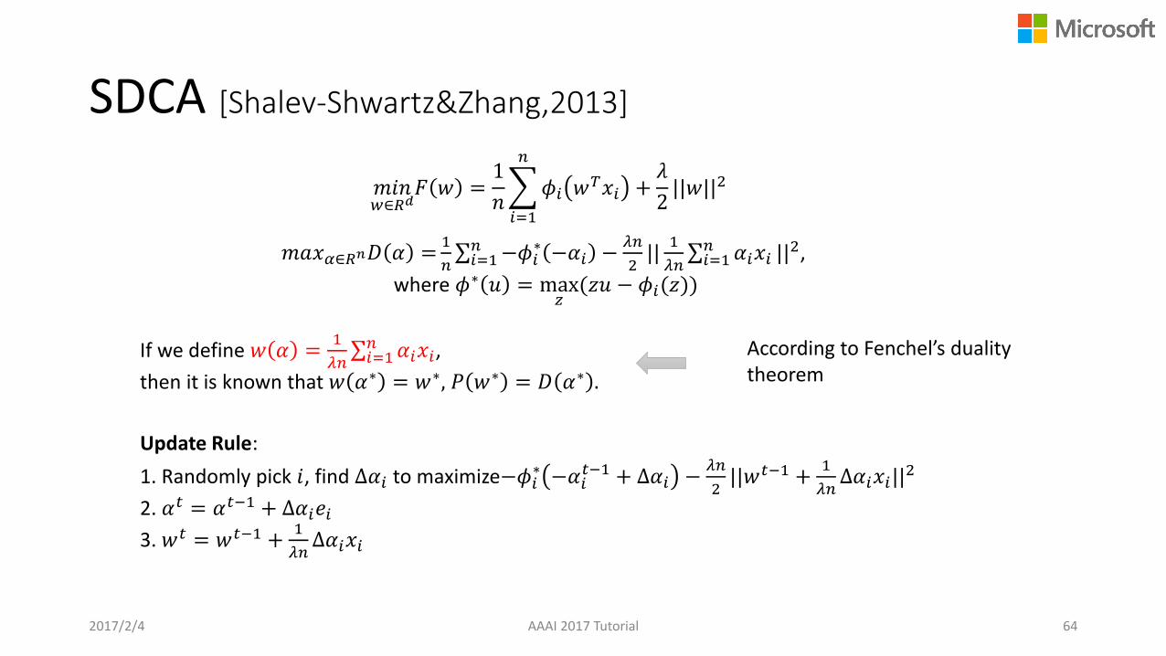
SDCA [Shalev-Shwartz&Zhang,2013]
𝑚𝑖𝑛𝑤∈𝑅𝑑
𝐹 𝑤 =1
𝑛
𝑖=1
𝑛
𝜙𝑖 𝑤𝑇𝑥𝑖 +
𝜆
2||𝑤||2
𝑚𝑎𝑥𝛼∈𝑅𝑛𝐷 𝛼 =1
𝑛σ𝑖=1𝑛 −𝜙𝑖
∗ −𝛼𝑖 −𝜆𝑛
2||
1
𝜆𝑛σ𝑖=1𝑛 𝛼𝑖𝑥𝑖 ||
2,
where 𝜙∗ 𝑢 = max𝑧(𝑧𝑢 − 𝜙𝑖(𝑧))
If we define 𝑤 𝛼 =1
𝜆𝑛σ𝑖=1𝑛 𝛼𝑖𝑥𝑖,
then it is known that 𝑤 𝛼∗ = 𝑤∗, 𝑃 𝑤∗ = 𝐷 𝛼∗ .
According to Fenchel’s duality theorem
Update Rule:
1. Randomly pick 𝑖, find Δ𝛼𝑖 to maximize−𝜙𝑖∗ −𝛼𝑖
𝑡−1 + Δ𝛼𝑖 −𝜆𝑛
2||𝑤𝑡−1 +
1
𝜆𝑛Δ𝛼𝑖𝑥𝑖||
2
2. 𝛼𝑡 = 𝛼𝑡−1 + Δ𝛼𝑖𝑒𝑖3. 𝑤𝑡 = 𝑤𝑡−1 +
1
𝜆𝑛Δ𝛼𝑖𝑥𝑖
2017/2/4 AAAI 2017 Tutorial 64

Convergence Rate of SDCA
2017/2/4 AAAI 2017 Tutorial 65
Complexity L-Lipschitz 𝜷-smooth
SDCA𝑂 𝑛 +
𝐿2
𝜆𝝐 𝑂 𝑛 +𝛽
𝜆log
1
𝝐
Assumption: 𝜙𝑖 is convex and 𝐿-Lipschitz or 𝛽 – smooth
It is well known that if 𝜙𝑖(𝛼) is 𝛽-smooth, then 𝜙𝑖∗(𝑢) is 1/𝛽-strongly convex.
where 𝜆 is the regularization term coefficient.
Stopping Criterion: Duality gap 𝐹 𝑤 𝛼 − 𝐷 𝛼 ≤ 𝜖
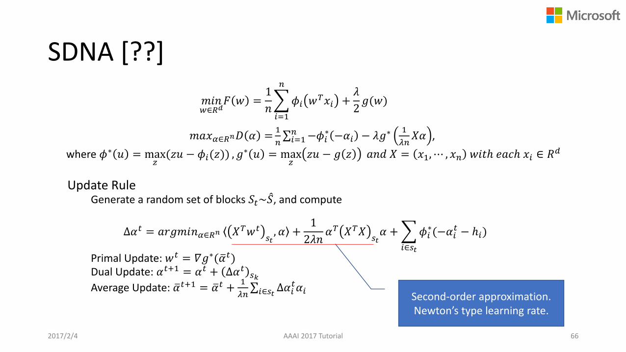
SDNA [??]
Update RuleGenerate a random set of blocks 𝑆𝑡~ መ𝑆, and compute
Δ𝛼𝑡 = 𝑎𝑟𝑔𝑚𝑖𝑛𝛼∈𝑅𝑛 𝑋𝑇𝑤𝑡𝑠𝑡, 𝛼 +
1
2𝜆𝑛𝛼𝑇 𝑋𝑇𝑋
𝑠𝑡𝛼 +
𝑖∈𝑠𝑡
𝜙𝑖∗(−𝛼𝑖
𝑡 − ℎ𝑖)
Primal Update: 𝑤𝑡 = 𝛻𝑔∗( ത𝛼𝑡)Dual Update: 𝛼𝑡+1 = 𝛼𝑡 + Δ𝛼𝑡 𝑠𝑘
Average Update: ത𝛼𝑡+1 = ത𝛼𝑡 +1
𝜆𝑛σ𝑖∈𝑠𝑡
Δ𝛼𝑖𝑡𝛼𝑖
2017/2/4 AAAI 2017 Tutorial 66
𝑚𝑖𝑛𝑤∈𝑅𝑑
𝐹 𝑤 =1
𝑛
𝑖=1
𝑛
𝜙𝑖 𝑤𝑇𝑥𝑖 +
𝜆
2𝑔(𝑤)
𝑚𝑎𝑥𝛼∈𝑅𝑛𝐷 𝛼 =1
𝑛σ𝑖=1𝑛 −𝜙𝑖
∗ −𝛼𝑖 − 𝜆𝑔∗1
𝜆𝑛𝑋𝛼 ,
where 𝜙∗ 𝑢 = max𝑧(𝑧𝑢 − 𝜙𝑖(𝑧)) , 𝑔
∗ 𝑢 = max𝑧
𝑧𝑢 − 𝑔 𝑧 𝑎𝑛𝑑 𝑋 = 𝑥1, ⋯ , 𝑥𝑛 𝑤𝑖𝑡ℎ 𝑒𝑎𝑐ℎ 𝑥𝑖 ∈ 𝑅𝑑
Second-order approximation. Newton’s type learning rate.
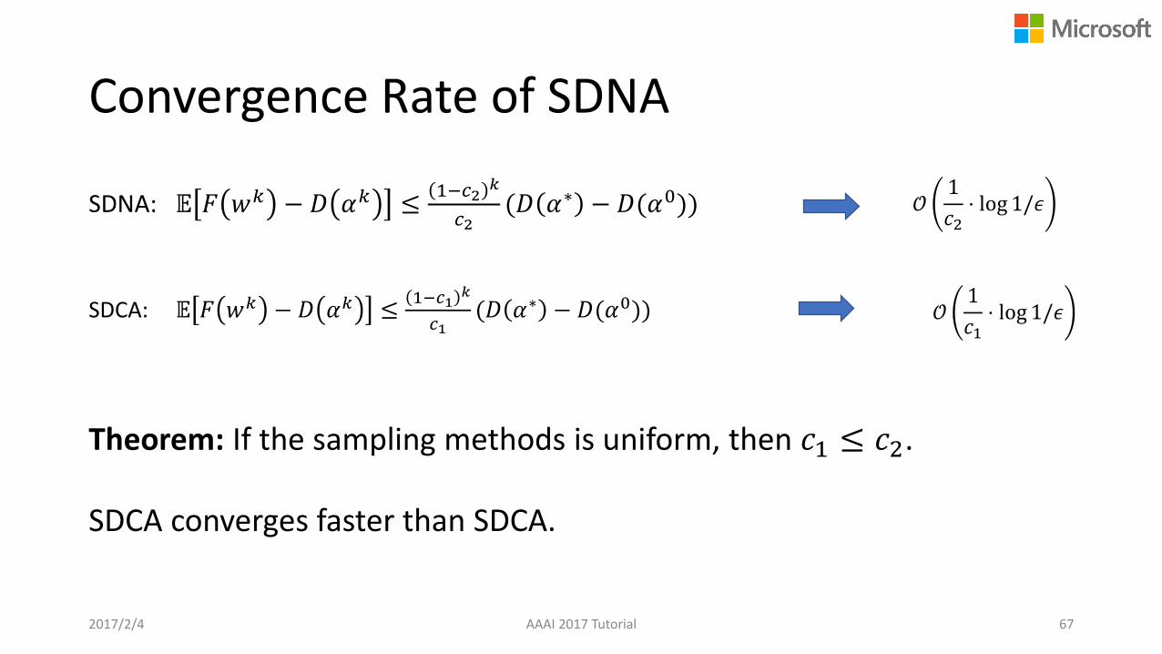
Convergence Rate of SDNA
SDNA: 𝔼 𝐹 𝑤𝑘 − 𝐷 𝛼𝑘 ≤1−𝑐2
𝑘
𝑐2(𝐷 𝛼∗ − 𝐷(𝛼0))
2017/2/4 AAAI 2017 Tutorial 67
SDCA: 𝔼 𝐹 𝑤𝑘 − 𝐷 𝛼𝑘 ≤1−𝑐1
𝑘
𝑐1(𝐷 𝛼∗ − 𝐷(𝛼0))
Theorem: If the sampling methods is uniform, then 𝑐1 ≤ 𝑐2.
SDCA converges faster than SDCA.
𝒪1
𝑐2⋅ log 1/𝜖
𝒪1
𝑐1⋅ log 1/𝜖
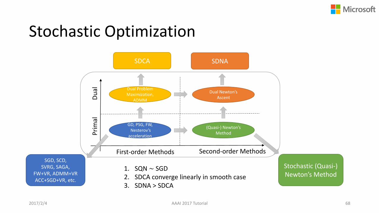
Stochastic Optimization
2017/2/4 AAAI 2017 Tutorial 68
First-order Methods Second-order Methods
GD, PSG, FW, Nesterov’s
accelerationPri
mal
Du
al Dual Problem Maximization,
ADMM
(Quasi-) Newton’s Method
Dual Newton’s Ascent
SGD, SCD, SVRG, SAGA,
FW+VR, ADMM+VRACC+SGD+VR, etc.
Stochastic (Quasi-) Newton’s Method
SDCA SDNA
1. SQN ∼ SGD2. SDCA converge linearly in smooth case3. SDNA > SDCA
2. Distributed Machine Learning: Foundations and Trends
2017/2/2 AAAI 2017 Tutorial 69

Data Parallelism vs. Model Parallelism
2017/2/2 AAAI 2017 Tutorial 70
1. Partition the training data2. Parallel training on different machines3. Synchronize the local updates4. Refresh local model with new parameters,
then go to 2.
1. Partition the model into multiple local workers 2. For every sample, the local workers collaborate
with each other to perform the optimization
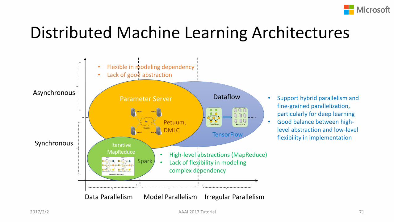
Distributed Machine Learning Architectures
AAAI 2017 Tutorial 71
Dataflow
Synchronous
Asynchronous
Data Parallelism Model Parallelism
Parameter Server
Irregular Parallelism
IterativeMapReduce • High-level abstractions (MapReduce)
• Lack of flexibility in modeling complex dependency
• Flexible in modeling dependency• Lack of good abstraction
• Support hybrid parallelism and fine-grained parallelization, particularly for deep learning
• Good balance between high-level abstraction and low-level flexibility in implementationTensorFlow
Petuum, DMLC
Spark
2017/2/2
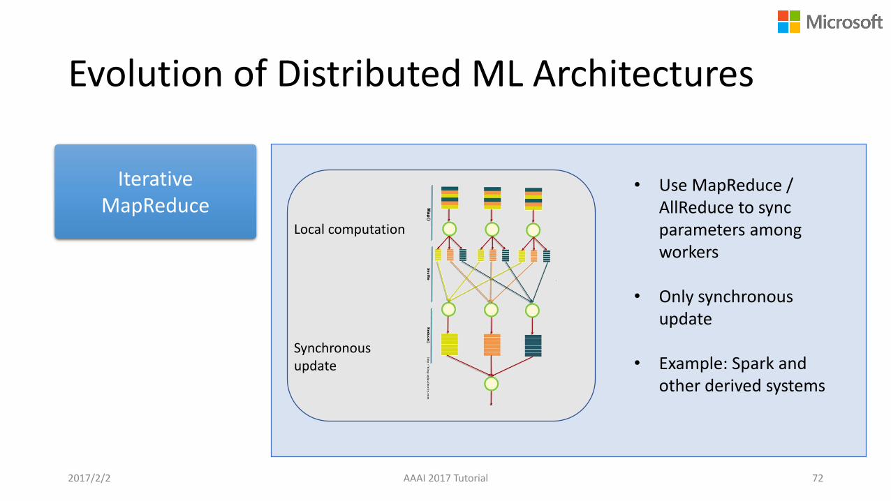
Evolution of Distributed ML Architectures
Iterative MapReduce
• Use MapReduce / AllReduce to sync parameters among workers
• Only synchronous update
• Example: Spark and other derived systems
Local computation
Synchronous update
2017/2/2 AAAI 2017 Tutorial 72
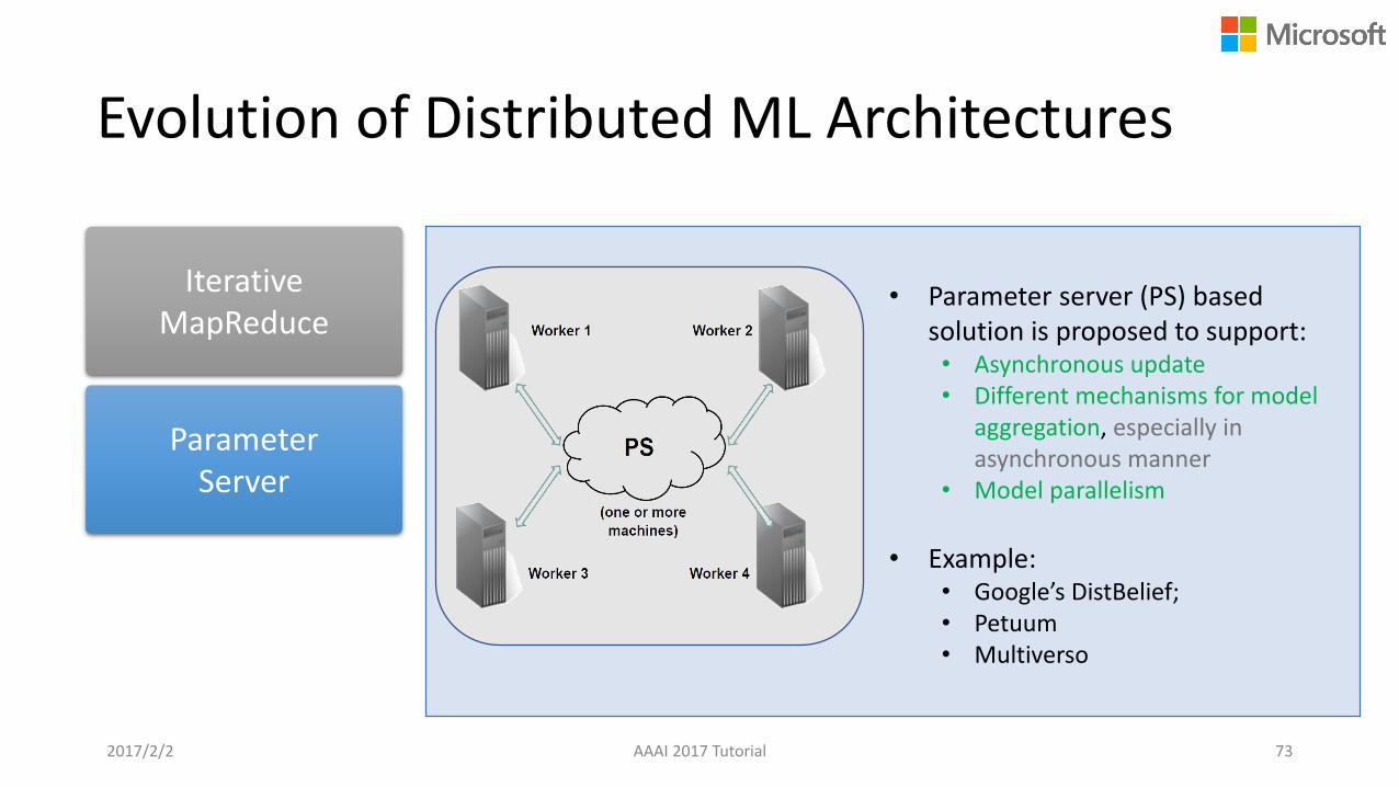
Evolution of Distributed ML Architectures
Iterative MapReduce
Parameter Server
• Parameter server (PS) based solution is proposed to support: • Asynchronous update• Different mechanisms for model
aggregation, especially in asynchronous manner
• Model parallelism
• Example: • Google’s DistBelief; • Petuum• Multiverso
2017/2/2 AAAI 2017 Tutorial 73

Evolution of Distributed ML Architectures
Iterative MapReduce
Parameter Server
Dataflow based solution is proposed to support:• Irregular parallelism (e.g., hybrid
data- and model-parallelism), particularly in deep learning
• Both high-level abstraction and low-level flexibility in implementation
Example: • TensorFlow
Dataflow
Task scheduling & execution based on: 1. Data dependency2. Resource availability
Dataflow Resource
2017/2/2 AAAI 2017 Tutorial 74

Data Parallelism
• Optimization under different parallelization mechanisms• Synchronous vs. Asynchronous vs. Lock-free
• Aggregation method• Consensus based on model average
• Data allocation strategy• Shuffling + Partition
• Sampling
2017/2/2 AAAI 2017 Tutorial 75

Parallelization Mechanism: BSP
2017/2/2 AAAI 2017 Tutorial 76
Bulk Synchronous Parallel

Example Algorithm: BSP-SGD
2017/2/2 AAAI 2017 Tutorial 77
Minibatch SGD [Dekel 𝑒𝑡. 𝑎𝑙.,2013]
Communication: every iteration
Convergence Rate: (convex and smooth case)
𝑂1
𝑃𝑇
Speedup: O 𝑃
min𝒘
𝑘=1
𝐾
𝐿𝑘 𝑤
𝑤𝑘𝑡 = 𝑤𝑡
∆𝑤𝑘𝑡 = −𝜂𝑡𝛻𝐿𝑘(𝑤𝑘
𝑡)
𝑤𝑡+1 = 𝑤𝑡 +
𝑘
∆𝑤𝑘𝑡
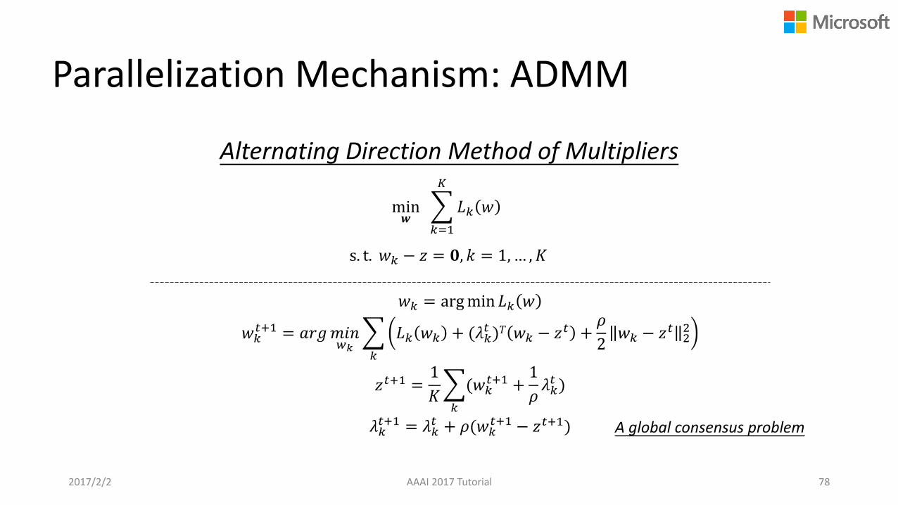
Parallelization Mechanism: ADMM
Alternating Direction Method of Multipliers
2017/2/2 AAAI 2017 Tutorial 78
min𝒘
𝑘=1
𝐾
𝐿𝑘 𝑤
s. t. 𝑤𝑘 − 𝑧 = 𝟎, 𝑘 = 1,… , 𝐾
𝑤𝑘 = argmin 𝐿𝑘 𝑤
𝑤𝑘𝑡+1 = 𝑎𝑟𝑔𝑚𝑖𝑛
𝑤𝑘
𝑘
𝐿𝑘 𝑤𝑘 + (𝜆𝑘𝑡 )𝑇 𝑤𝑘 − 𝑧𝑡 +
𝜌
2𝑤𝑘 − 𝑧𝑡 2
2
𝑧𝑡+1 =1
𝐾
𝑘
(𝑤𝑘𝑡+1 +
1
𝜌𝜆𝑘𝑡 )
𝜆𝑘𝑡+1 = 𝜆𝑘
𝑡 + 𝜌(𝑤𝑘𝑡+1 − 𝑧𝑡+1) A global consensus problem
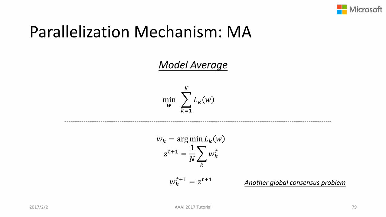
Parallelization Mechanism: MA
Model Average
2017/2/2 AAAI 2017 Tutorial 79
𝑤𝑘 = argmin 𝐿𝑘 𝑤
𝑧𝑡+1 =1
𝑁
𝑘
𝑤𝑘𝑡
𝑤𝑘𝑡+1 = 𝑧𝑡+1
min𝒘
𝑘=1
𝐾
𝐿𝑘 𝑤
Another global consensus problem
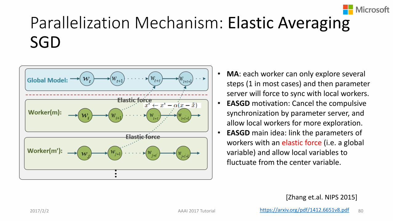
Parallelization Mechanism: Elastic Averaging SGD
2017/2/2 AAAI 2017 Tutorial 80
• MA: each worker can only explore several steps (1 in most cases) and then parameter server will force to sync with local workers.
• EASGD motivation: Cancel the compulsive synchronization by parameter server, and allow local workers for more exploration.
• EASGD main idea: link the parameters of workers with an elastic force (i.e. a global variable) and allow local variables to fluctuate from the center variable.
https://arxiv.org/pdf/1412.6651v8.pdf
[Zhang et.al. NIPS 2015]

Worker 1
Worker 2
Worker 3
Worker 4
∆𝜔12 𝜔
Time
Parameter Server
Workers push update to parameter server and/or pull latest parameter back without waiting for others
Parallelization Mechanism: ASP
2017/2/2 AAAI 2017 Tutorial 81
Asynchronous Parallel
Example Algorithm: ASGD
2017/2/2 AAAI 2017 Tutorial 82
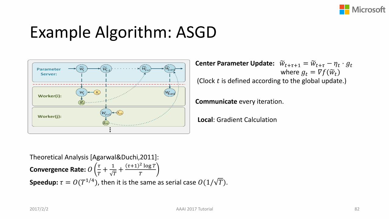
Center Parameter Update: 𝑤𝑡+𝜏+1 = 𝑤𝑡+𝜏 − 𝜂𝑡 ⋅ 𝑔𝑡where 𝑔𝑡 = 𝛻𝑓(𝑤𝑡)
(Clock 𝑡 is defined according to the global update.)
Local: Gradient Calculation
Theoretical Analysis [Agarwal&Duchi,2011]:
Convergence Rate: 𝑂𝜏
𝑇+
1
𝑇+
𝜏+1 2 log 𝑇
𝑇
Speedup: 𝜏 = 𝑂(𝑇1/4), then it is the same as serial case 𝑂(1/ 𝑇).
Communicate every iteration.

Parallelization Mechanism: AADMM
Asynchronous ADMM
• Partial barrier and bounded delay
• Each local machine updates 𝑤 using the most recent 𝑧 received from the server
• The server update 𝑧 after receiving 𝑆not-too-old updates from the local machines.
2017/2/2 AAAI 2017 Tutorial 83

Parallelization Mechanism: Hogwild!
Goal: min𝑓 𝑥 = σ𝑒∈𝐸 𝑓𝑒(𝑥𝑒) hypergraph 𝐺(𝑉, 𝐸). Each subvector 𝑥𝑒 induces an edge consisting of some nodes (training instances).
Three sparse parameter:
Ω = max𝑒∈_𝐸
|𝑒|, Δ =max1≤𝑣≤𝑛
𝑒∈𝐸:𝑣∈𝑒
|𝐸|, 𝜌 =
max𝑒∈𝐸
Ƹ𝑒∈𝐸:𝑒∩ Ƹ𝑒≠∅
|𝐸|
Theoretical Analysis: with-lock, constant learning rate
If 𝜏 = 𝑜(𝑛1/4) as 𝜌 and Δ are typically both 𝑜1
𝑛, it can achieve linear speedup.
Lock-free implementation in shared memory!
[Niu et al,NIPS-11]
2017/2/2 AAAI 2017 Tutorial 84

Parallelization Mechanism: Cyclades
𝐺𝑢 𝐺𝑐
Cyclades samples updates 𝑢𝑖 and Finds conflict-groups.
Allocation: processing all the conflicting updates within the same core
Processing a batch is completed.
Δ: the max vertexdegree of 𝐺𝑐
𝐸𝑢: the number of edges of 𝐺𝑢
Theoretical Results: Cyclades on 𝑃 = 𝑂𝑛
Δ⋅Δ𝐿cores, with batch sizes 𝐵 =
1−𝜖 𝑛
Δcan execute 𝑇 = 𝑐 ⋅ 𝑛 updates, for any constant 𝑐 ≥ 1,
selected uniformly at random with replacement, in time 𝑂𝐸𝑢⋅𝜆
𝑃⋅ log2 𝑛 with high probability, where 𝜆 is a constant.
Motivation: introduce no conflicts between cores during the asynchronous parallel execution.
[Pan, et al, NIPS-16]2017/2/2 AAAI 2017 Tutorial 85

• In theory - full access• Online accessing: 𝑖𝑡~𝑃 i.i.d
• Full access + with replacement sampling
• In practice - random shuffling + data partition + local sampling with replacement• One-shot SGD [Zhang 𝑒𝑡. 𝑎𝑙. 2012]
• Shuffling + partition: statistical similarity
• Other algorithms e.g. ADMM has convergence guarantee
2017/2/2 AAAI 2017 Tutorial 86
Data Allocation Strategy
Data Parallelism vs. Model Parallelism
2017/2/2 AAAI 2017 Tutorial 87
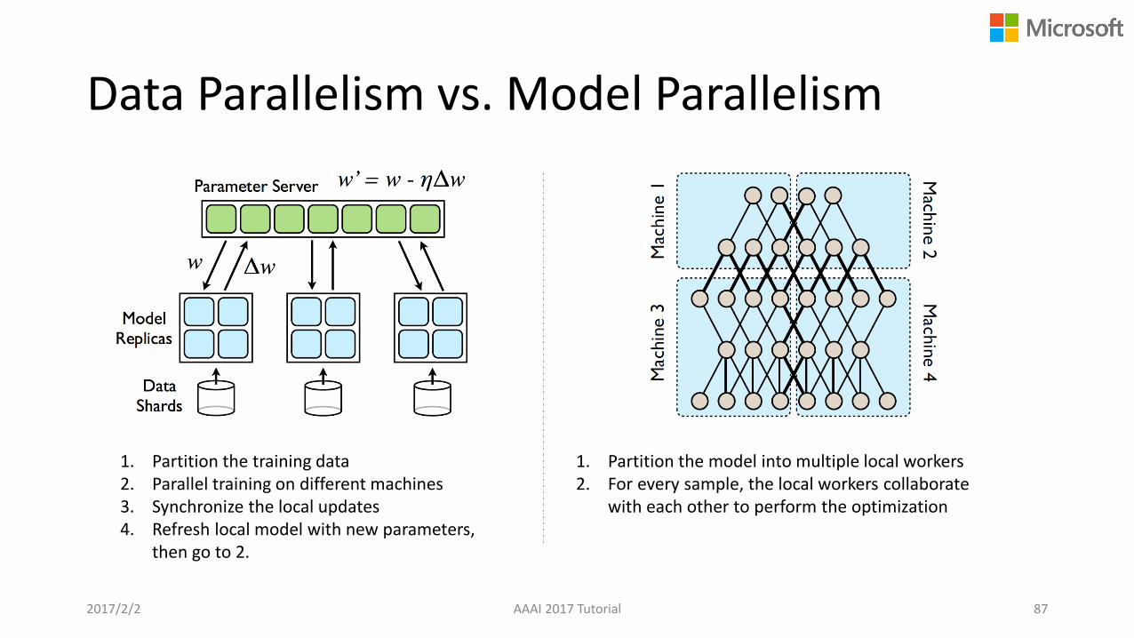
1. Partition the training data2. Parallel training on different machines3. Synchronize the local updates4. Refresh local model with new parameters,
then go to 2.
1. Partition the model into multiple local workers 2. For every sample, the local workers collaborate
with each other to perform the optimization
Model Parallelism
• Synchronous model parallelization
• Asynchronous model slicing
• Model parallelization with model block scheduling
2017/2/2 AAAI 2017 Tutorial 88
Synchronous Model Parallelization
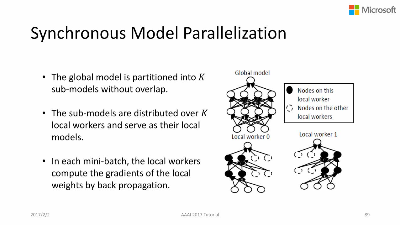
• The global model is partitioned into 𝐾sub-models without overlap.
• The sub-models are distributed over 𝐾local workers and serve as their local models.
• In each mini-batch, the local workers compute the gradients of the local weights by back propagation.
2017/2/2 AAAI 2017 Tutorial 89
Synchronous Model Parallelization
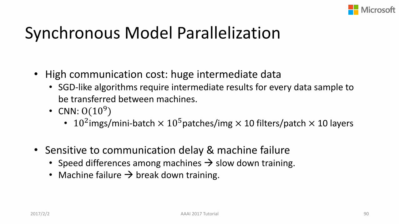
2017/2/2 AAAI 2017 Tutorial 90
• High communication cost: huge intermediate data• SGD-like algorithms require intermediate results for every data sample to
be transferred between machines.• CNN: O(109)
• 102imgs/mini-batch × 105patches/img × 10 filters/patch × 10 layers
• Sensitive to communication delay & machine failure• Speed differences among machines slow down training.• Machine failure break down training.

Asynchronous Model Slicing
Intermediate Data
𝑤𝑖,𝑗 ∈ 𝑠𝑙𝑖𝑐𝑒1
Multiverso server
e.g., activations in DNN, Doc-topic table in LDA
𝑤𝑖,𝑗 ∈ 𝑠𝑙𝑖𝑐𝑒2
Stochastic Coordinate Descent (SCD)
Timeline
Other activations are retrieved from historical storage in local machine
Parameters in the slice and hidden-node
activations triggered by the slice are updated.
𝑡1 𝑡2
When updating Slice1, previous
information about Slice2 is reused.
when updating Slice2, previous
information about Slice1 is reused.
• Model slices are pulled from server and updated in a round robin fashion.
Client
Server
2017/2/2 AAAI 2017 Tutorial 91
2017/2/2 AAAI 2017 Tutorial 92
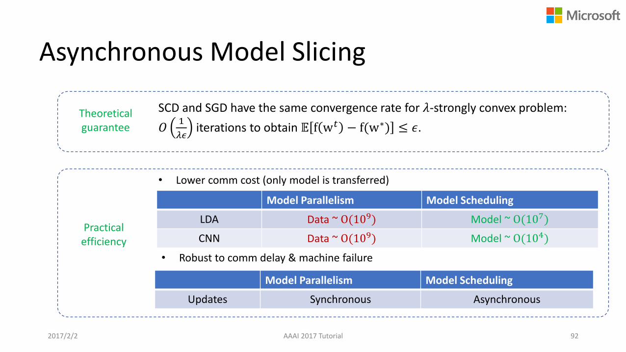
Asynchronous Model Slicing
• Lower comm cost (only model is transferred)
SCD and SGD have the same convergence rate for 𝜆-strongly convex problem:
𝑂1
𝜆𝜖iterations to obtain 𝔼 f w𝑡 − f(w∗) ≤ 𝜖.
• Robust to comm delay & machine failure
Model Parallelism Model Scheduling
LDA Data ~ O(109) Model ~ O(107)
CNN Data ~ O(109) Model ~ O(104)
Theoretical guarantee
Practical efficiency
Model Parallelism Model Scheduling
Updates Synchronous Asynchronous
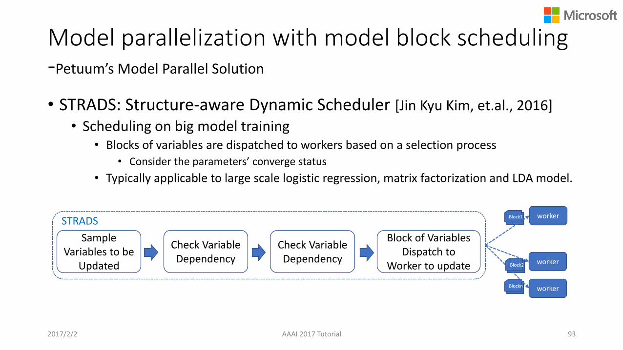
• STRADS: Structure-aware Dynamic Scheduler [Jin Kyu Kim, et.al., 2016]
• Scheduling on big model training• Blocks of variables are dispatched to workers based on a selection process
• Consider the parameters’ converge status
• Typically applicable to large scale logistic regression, matrix factorization and LDA model.
Model parallelization with model block scheduling-Petuum’s Model Parallel Solution
2017/2/2 AAAI 2017 Tutorial 93
Check Variable Dependency
Block of Variables Dispatch to
Worker to update
Check Variable Dependency
Sample Variables to be
Updated
STRADSworkerBlock1
worker
workerBlock2
Blockn

2. Distributed Machine Learning:Foundations and Trends
2017/2/4 AAAI 2017 Tutorial 94
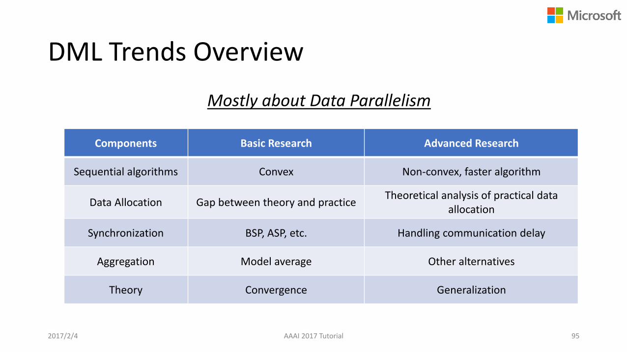
DML Trends Overview
2017/2/4 AAAI 2017 Tutorial 95
Mostly about Data Parallelism
Components Basic Research Advanced Research
Sequential algorithms Convex Non-convex, faster algorithm
Data Allocation Gap between theory and practiceTheoretical analysis of practical data
allocation
Synchronization BSP, ASP, etc. Handling communication delay
Aggregation Model average Other alternatives
Theory Convergence Generalization
Distributed ML Recent Advances
• Faster Stochastic Optimization Methods
• Non-convex Optimization
• Theoretical Analysis of Practical Data Allocation
• Handling Communication Delay
• Alternative Aggregation Methods
• Generalization Theory
2017/2/4 AAAI 2017 Tutorial 96

SVRG
Initialize 𝑥0Iterate: for s=1,2…
𝑥 = 𝑥𝑠−1𝑢 =
1
𝑛σ𝑖=1𝑛 𝛻𝑓𝑖( 𝑥)
𝑥0 = 𝑥Iterate: for 𝑡 = 1,2, … ,𝑚
Randomly pick 𝑖𝑡 ∈ {1,… , 𝑛} and update weight𝑥𝑡 = 𝑥𝑡−1 − 𝜂(𝛻𝑓𝑖𝑡 𝑥𝑡−1 − 𝛻𝑓𝑖𝑡 𝑥 + 𝑢)
endOption 1: set 𝑥𝑠 = 𝑥𝑚Option 2: set 𝑥𝑠 = 𝑥𝑡 for randomly chosen 𝑡.
end
VR-regularized Gradient:𝑣𝑡 = 𝛻𝑓𝑖𝑡 𝑥𝑡−1 − 𝛻𝑓𝑖𝑡 𝑥 + 𝑢
𝐸𝑖𝑡||𝑣𝑡||2 ≤ 4𝐿 𝑓 𝑥𝑡−1 − 𝑓 𝑥∗ + 𝑓 𝑥 − 𝑓 𝑥∗
With 𝑥𝑡 → 𝑥∗, 𝐸𝑖𝑡||𝑣𝑡||2 → 0.
Error Induction:𝐸 𝑓 𝑥𝑠 − 𝑓 𝑥∗
≤1
𝛼𝜂 1 − 2𝛽𝜂 𝑚+
2𝛽𝜂
1 − 2𝛽𝜂𝐸[𝑓 𝑥𝑠−1 − 𝑓(𝑥∗)]
With 𝜂 =𝑐
𝛽, 𝑚 = 𝑂
𝛽
𝛼
Linear ConvergenceExtra computation: 1. Full gradient 𝒖2. Random gradient of 𝒙
2017/2/4 AAAI 2017 Tutorial 97[Johnson&Zhang 2013]
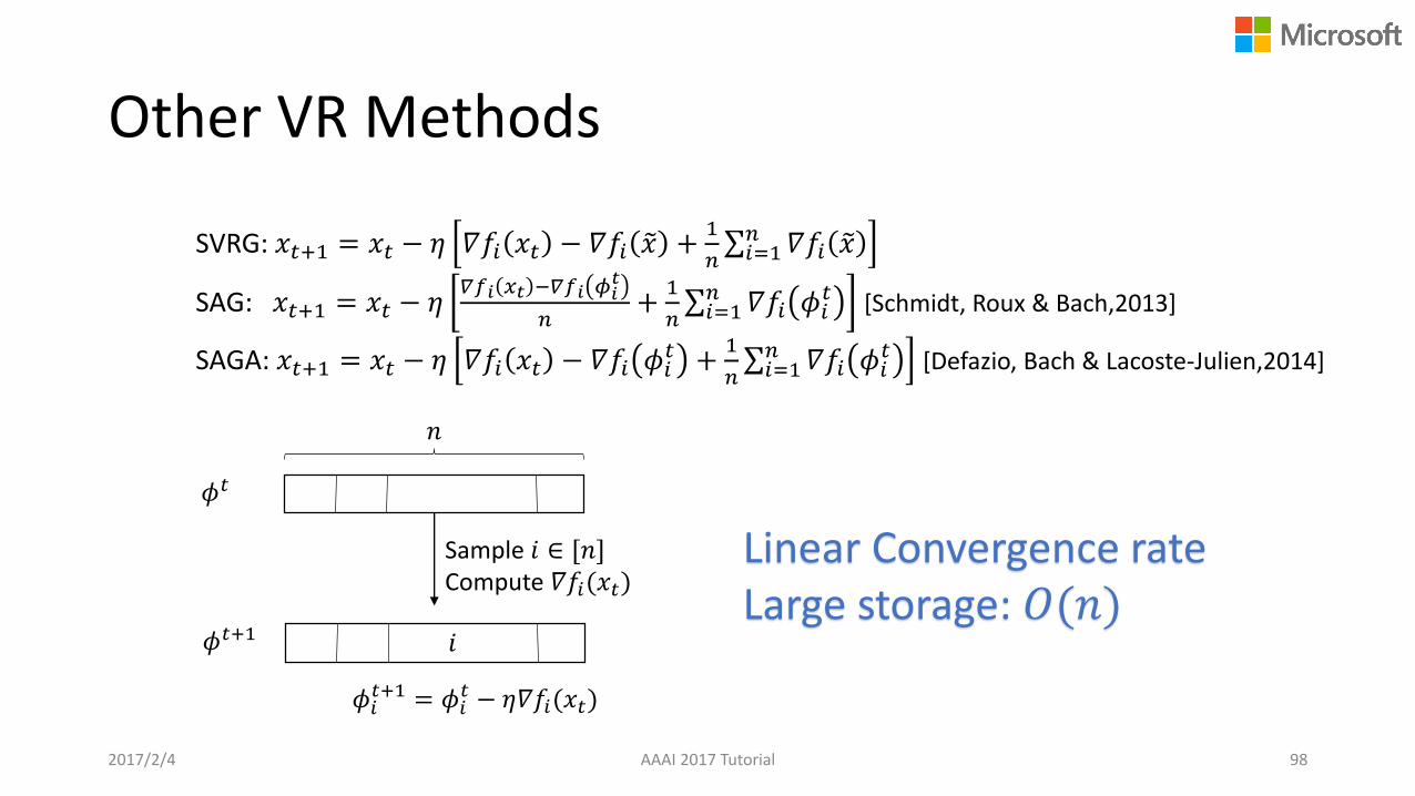
Other VR Methods
2017/2/4 AAAI 2017 Tutorial 98
SVRG: 𝑥𝑡+1 = 𝑥𝑡 − 𝜂 𝛻𝑓𝑖 𝑥𝑡 − 𝛻𝑓𝑖 𝑥 +1
𝑛σ𝑖=1𝑛 𝛻𝑓𝑖 𝑥
SAG: 𝑥𝑡+1 = 𝑥𝑡 − 𝜂𝛻𝑓𝑖 𝑥𝑡 −𝛻𝑓𝑖 𝜙𝑖
𝑡
𝑛+
1
𝑛σ𝑖=1𝑛 𝛻𝑓𝑖 𝜙𝑖
𝑡 [Schmidt, Roux & Bach,2013]
SAGA: 𝑥𝑡+1 = 𝑥𝑡 − 𝜂 𝛻𝑓𝑖 𝑥𝑡 − 𝛻𝑓𝑖 𝜙𝑖𝑡 +
1
𝑛σ𝑖=1𝑛 𝛻𝑓𝑖 𝜙𝑖
𝑡 [Defazio, Bach & Lacoste-Julien,2014]
𝜙𝑡
𝑛
Sample 𝑖 ∈ [𝑛]Compute 𝛻𝑓𝑖(𝑥𝑡)
𝜙𝑡+1 𝑖
𝜙𝑖𝑡+1 = 𝜙𝑖
𝑡 − 𝜂𝛻𝑓𝑖(𝑥𝑡)
Linear Convergence rateLarge storage: 𝑂(𝑛)
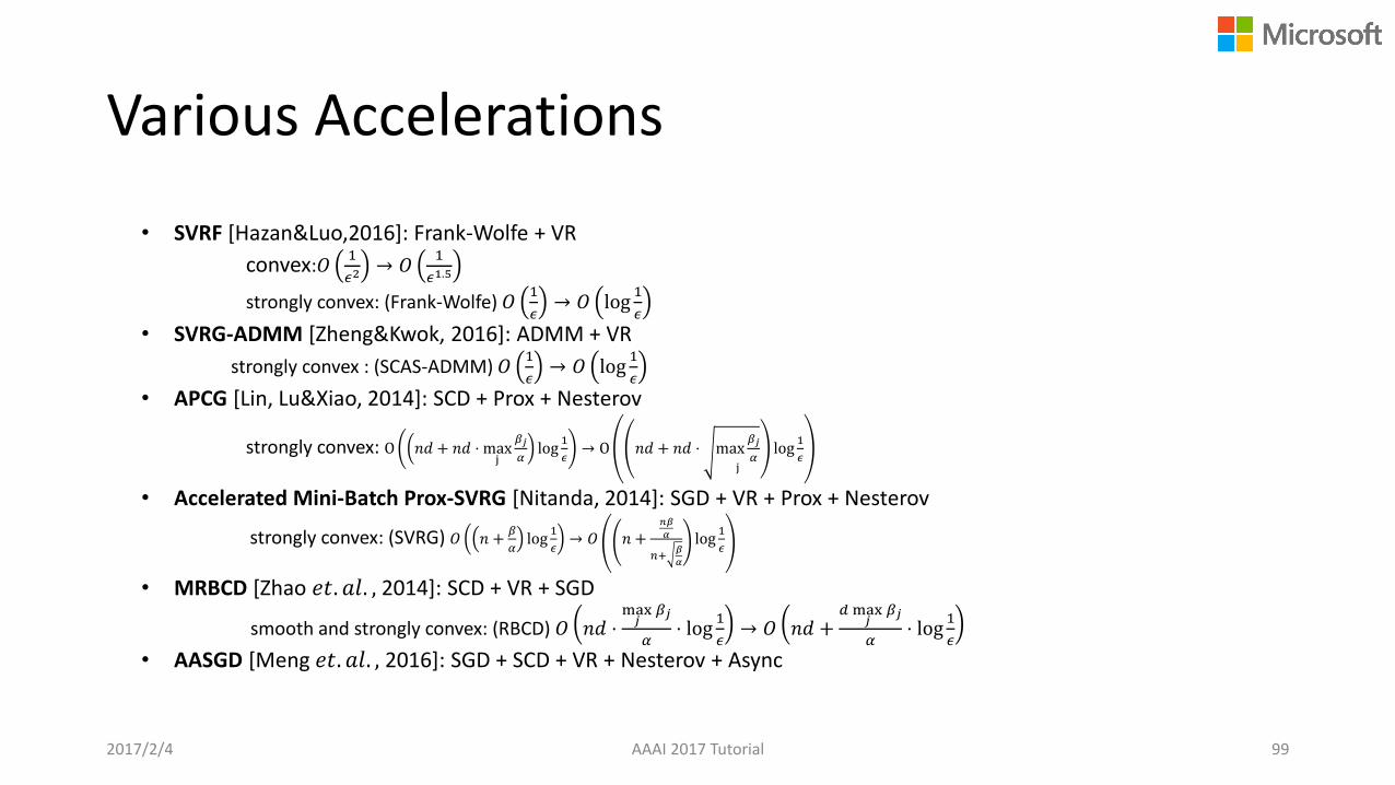
Various Accelerations
2017/2/4 AAAI 2017 Tutorial 99
• SVRF [Hazan&Luo,2016]: Frank-Wolfe + VR
convex:𝑂1
𝜖2→ 𝑂
1
𝜖1.5
strongly convex: (Frank-Wolfe) 𝑂1
𝜖→ 𝑂 log
1
𝜖
• SVRG-ADMM [Zheng&Kwok, 2016]: ADMM + VR
strongly convex : (SCAS-ADMM) 𝑂1
𝜖→ 𝑂 log
1
𝜖
• APCG [Lin, Lu&Xiao, 2014]: SCD + Prox + Nesterov
strongly convex: O 𝑛𝑑 + 𝑛𝑑 ⋅ maxj
𝛽𝑗
𝛼log
1
𝜖→ O 𝑛𝑑 + 𝑛𝑑 ⋅ max
𝛽𝑗
𝛼j
log1
𝜖
• Accelerated Mini-Batch Prox-SVRG [Nitanda, 2014]: SGD + VR + Prox + Nesterov
strongly convex: (SVRG) 𝑂 𝑛 +𝛽
𝛼log
1
𝜖→ 𝑂 𝑛 +
𝑛𝛽
𝛼
𝑛+𝛽
𝛼
log1
𝜖
• MRBCD [Zhao 𝑒𝑡. 𝑎𝑙. , 2014]: SCD + VR + SGD
smooth and strongly convex: (RBCD) 𝑂 𝑛𝑑 ⋅max𝑗
𝛽𝑗
𝛼⋅ log
1
𝜖→ 𝑂 𝑛𝑑 +
𝑑 max𝑗
𝛽𝑗
𝛼⋅ log
1
𝜖
• AASGD [Meng 𝑒𝑡. 𝑎𝑙. , 2016]: SGD + SCD + VR + Nesterov + Async

Asynchronous Accelerated SGD (AASGD)Variance
Reduction(VR)
Nesterov’sAcceleration
(NA)
AsynchronousParallelism
Coordinate Sampling
(CS)
…….
Master
Worker 1 Worker 2 Worker P
Key problem: Delayed gradients𝑀𝑜𝑑𝑒𝑙𝑡+1 = 𝑈𝑝𝑑𝑎𝑡𝑒 (𝑀𝑜𝑑𝑒𝑙𝑡, 𝐺𝑟𝑎𝑑𝑖𝑒𝑛𝑡𝑡−𝜏)
Worker: Gradient Aggregation
Master Parameter Update
Master:Gradient computing
Push gradients
Pull Master parameters
2017/2/4 AAAI 2017 Tutorial 100
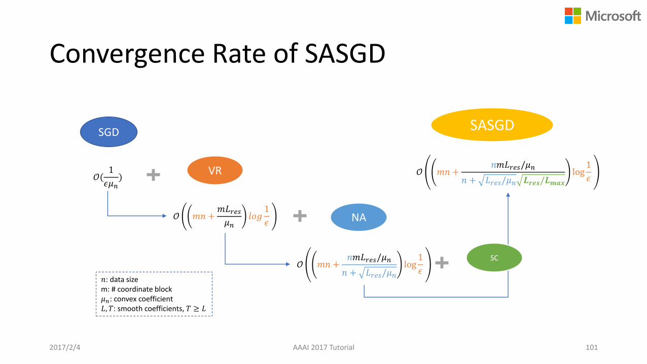
Convergence Rate of SASGD
𝒪(1
𝜖𝜇𝑛)
VR
𝒪 𝑚𝑛 +𝑚𝐿𝑟𝑒𝑠𝜇𝑛
𝑙𝑜𝑔1
𝜖 NA
𝒪 𝑚𝑛 +𝑛𝑚𝐿𝑟𝑒𝑠/𝜇𝑛
𝑛 + 𝐿𝑟𝑒𝑠/𝜇𝑛log
1
𝜖
SC
𝒪 𝑚𝑛 +𝑛𝑚𝐿𝑟𝑒𝑠/𝜇𝑛
𝑛 + 𝐿𝑟𝑒𝑠/𝜇𝑛 𝑳𝒓𝒆𝒔/𝑳𝒎𝒂𝒙
log1
𝜖
SGD SASGD
𝑛: data sizem: # coordinate block𝜇𝑛: convex coefficient𝐿, 𝑇: smooth coefficients, 𝑇 ≥ 𝐿
2017/2/4 AAAI 2017 Tutorial 101
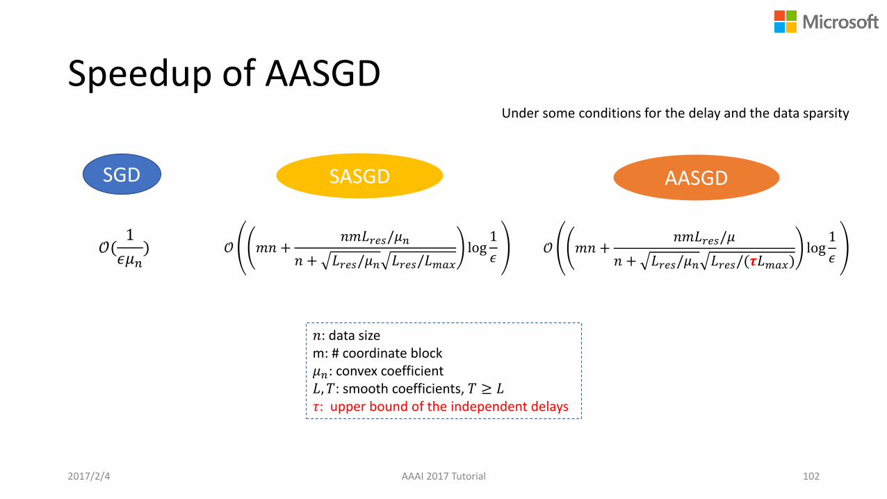
Speedup of AASGD
𝒪(1
𝜖𝜇𝑛) 𝒪 𝑚𝑛 +
𝑛𝑚𝐿𝑟𝑒𝑠/𝜇𝑛
𝑛 + 𝐿𝑟𝑒𝑠/𝜇𝑛 𝐿𝑟𝑒𝑠/𝐿𝑚𝑎𝑥
log1
𝜖
SGD SASGD
𝒪 𝑚𝑛 +𝑛𝑚𝐿𝑟𝑒𝑠/𝜇
𝑛 + 𝐿𝑟𝑒𝑠/𝜇𝑛 𝐿𝑟𝑒𝑠/(𝝉𝐿𝑚𝑎𝑥)log
1
𝜖
AASGD
𝑛: data sizem: # coordinate block𝜇𝑛: convex coefficient𝐿, 𝑇: smooth coefficients, 𝑇 ≥ 𝐿𝜏: upper bound of the independent delays
Under some conditions for the delay and the data sparsity
2017/2/4 AAAI 2017 Tutorial 102
Distribute ML Recent Advances
• Faster Stochastic Optimization Methods
• Non-convex Optimization
• Theoretical Analysis of Practical Data Allocation
• Handling Communication Delay
• Alternative Aggregation Methods
• Generalization Theory
2017/2/4 AAAI 2017 Tutorial 103
Non-convex Optimization
• Tasks:• Training of deep neural networks• Inference in graphical models• Unsupervised learning models, such as topic models, dictionary learning.
• In general, the global optimization of a non-convex function is NP-hard.
• Approaches:• Under some assumptions on the input for some models, we can design specific
polynomial-time algorithms.• Robust, generic algorithms: simulated annealing, Bayesian optimization usually
perform well in practice.• Attempt to reach a stationary point.• Graduated Optimization
2017/2/4 AAAI 2017 Tutorial 104
Attempt to Reach a Stationary Point
2017/2/4 AAAI 2017 Tutorial 105
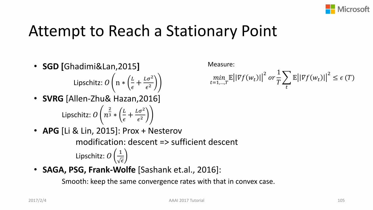
• SGD [Ghadimi&Lan,2015]
Lipschitz: 𝑂 n ∗𝐿
𝜖+
𝐿𝜎2
𝜖2
• SVRG [Allen-Zhu& Hazan,2016]
Lipschitz: 𝑂 𝑛2
3 ∗𝐿
𝜖+
𝐿𝜎2
𝜖2
• APG [Li & Lin, 2015]: Prox + Nesterovmodification: descent => sufficient descent
Lipschitz: 𝑂1
𝜖
• SAGA, PSG, Frank-Wolfe [Sashank et.al., 2016]:Smooth: keep the same convergence rates with that in convex case.
Measure:
𝑚𝑖𝑛𝑡=1,…,𝑇
𝔼 𝛻𝑓 𝑤𝑡2𝑜𝑟
1
𝑇
𝑡
𝔼 𝛻𝑓 𝑤𝑡2≤ 𝜖 (𝑇)
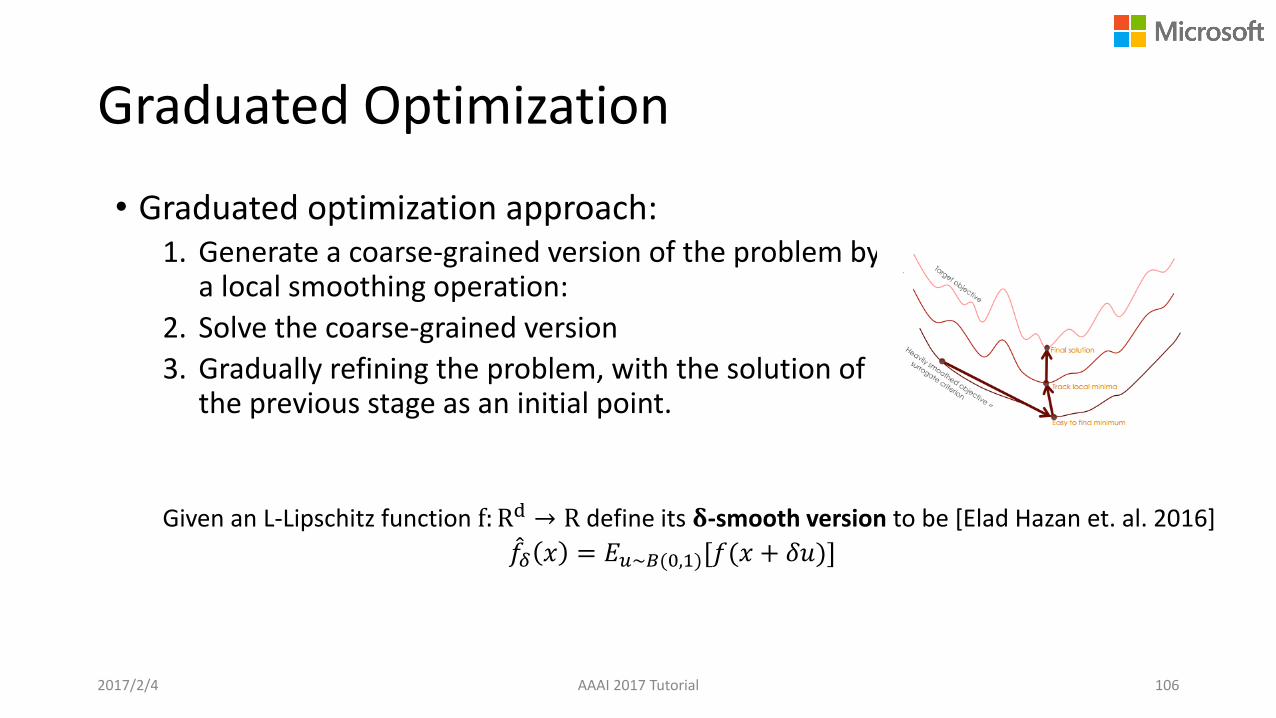
• Graduated optimization approach: 1. Generate a coarse-grained version of the problem by
a local smoothing operation:
2. Solve the coarse-grained version
3. Gradually refining the problem, with the solution of the previous stage as an initial point.
Graduated Optimization
2017/2/4 AAAI 2017 Tutorial 106
Given an L-Lipschitz function f: Rd → R define its 𝛅-smooth version to be [Elad Hazan et. al. 2016] መ𝑓𝛿 𝑥 = 𝐸𝑢~𝐵(0,1)[𝑓(𝑥 + 𝛿𝑢)]

Graduated Optimization
Generalized mollifiers {𝑇𝜎𝑓: 𝜎 > 0}: [Caglar Gulcehre, Yoshua Bengio, et al, 2016]lim𝜎→∞
𝑇𝜎𝑓 = 𝑓0 is an identity function,
lim𝜎→0
𝑇𝜎𝑓 = 𝑓,
𝜕 𝑇𝜎𝑓 𝑥
𝜕𝑥exists, ∀𝑥, 𝜎 > 0
Noisy mollifier: 𝑇𝜎𝑓 𝑥 = 𝐸𝜉[𝜙(𝑥, 𝜉𝜎)]
Noisy Mollifiers for NN: the random variable 𝜉𝜎 yields noise to activations in each layer, except the output layer. As 𝜎 becomes larger:• The nonlinearities → Linear• Complex input-output mapping → Identity, • Stochastic depth
Distribute ML Recent Advances
• Faster Stochastic Optimization Methods
• Non-convex Optimization
• Theoretical Analysis of Practical Data Allocation
• Handling Communication Delay
• Alternative Aggregation Methods
• Generalization Theory
2017/2/4 AAAI 2017 Tutorial 108
• In theory - full access• Online accessing: 𝑖𝑡~𝑃 i.i.d
• Full access + with replacement sampling
• In practice - random shuffling + data partition + local re-shuffling when the data is processed• One-shot SGD [Zhang 𝑒𝑡. 𝑎𝑙. 2012]
• Shuffling + partition: statistical similarity
• Other algorithms e.g. ADMM has convergence guarantee
2017/2/4 AAAI 2017 Tutorial 109
Recall: Gap between Theory and Practice
Without-Replacement Sampling
2017/2/4 AAAI 2017 Tutorial 110
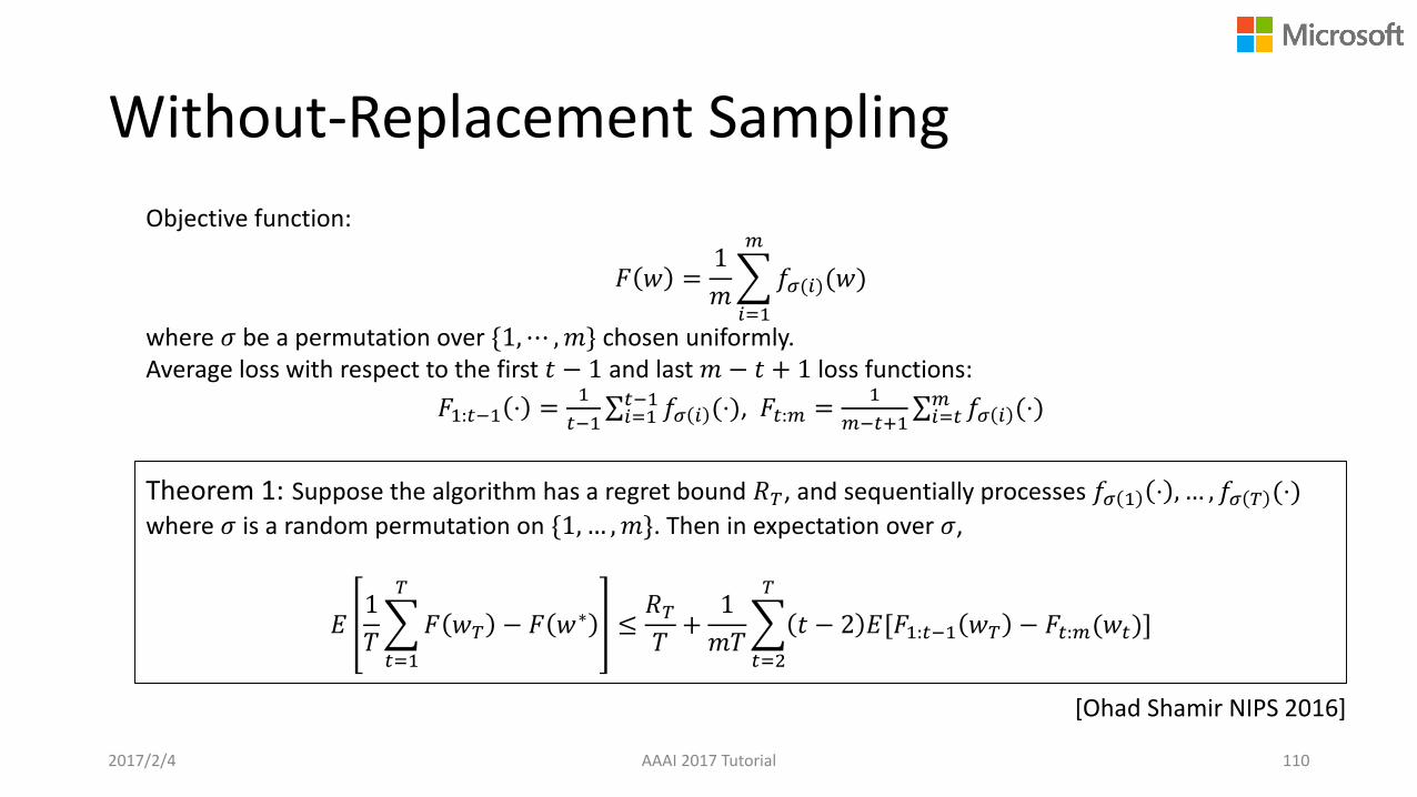
Objective function:
𝐹 𝑤 =1
𝑚
𝑖=1
𝑚
𝑓𝜎(𝑖)(𝑤)
where 𝜎 be a permutation over {1,⋯ ,𝑚} chosen uniformly.Average loss with respect to the first 𝑡 − 1 and last 𝑚 − 𝑡 + 1 loss functions:
𝐹1:𝑡−1 ⋅ =1
𝑡−1σ𝑖=1𝑡−1𝑓𝜎 𝑖 (⋅), 𝐹𝑡:𝑚 =
1
𝑚−𝑡+1σ𝑖=𝑡𝑚 𝑓𝜎 𝑖 (⋅)
Theorem 1: Suppose the algorithm has a regret bound 𝑅𝑇, and sequentially processes 𝑓𝜎 1 ⋅ , … , 𝑓𝜎 𝑇 (⋅)
where 𝜎 is a random permutation on {1, … ,𝑚}. Then in expectation over 𝜎,
𝐸1
𝑇
𝑡=1
𝑇
𝐹 𝑤𝑇 − 𝐹 𝑤∗ ≤𝑅𝑇𝑇+
1
𝑚𝑇
𝑡=2
𝑇
𝑡 − 2 𝐸[𝐹1:𝑡−1 𝑤𝑇 − 𝐹𝑡:𝑚(𝑤𝑡)]
[Ohad Shamir NIPS 2016]
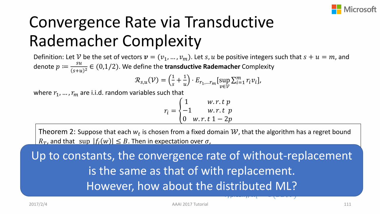
Convergence Rate via TransductiveRademacher Complexity
2017/2/4 AAAI 2017 Tutorial 111
Definition: Let 𝒱 be the set of vectors 𝒗 = (𝑣1, … , 𝑣𝑚). Let 𝑠, 𝑢 be positive integers such that 𝑠 + 𝑢 = 𝑚, and
denote 𝑝 ≔𝑠𝑢
𝑠+𝑢 2 ∈ (0,1/2). We define the transductive Rademacher Complexity
ℛ𝑠,𝑢 𝒱 =1
𝑠+
1
𝑢⋅ 𝐸𝑟1,…𝑟𝑚[sup
𝑣∈𝒱σ𝑖=1𝑚 𝑟𝑖𝑣𝑖],
where 𝑟1, … , 𝑟𝑚 are i.i.d. random variables such that
𝑟𝑖 = ቐ
1 𝑤. 𝑟. 𝑡 𝑝−1 𝑤. 𝑟. 𝑡 𝑝0 𝑤. 𝑟. 𝑡 1 − 2𝑝
Theorem 2: Suppose that each 𝑤𝑡 is chosen from a fixed domain 𝒲, that the algorithm has a regret bound
𝑅𝑇, and that sup𝑖,𝑤∈𝒲
𝑓𝑖 𝑤 ≤ 𝐵. Then in expectation over 𝜎,
𝐸1
𝑇
𝑡=1
𝑇
𝐹 𝑤𝑇 − 𝐹 𝑤∗ ≤𝑅𝑇𝑇+
1
𝑚𝑇
𝑡=2
𝑇
𝑡 − 1 ℛ𝑡−1:𝑚−𝑡+1 𝒱 +24𝐵
𝑚,
where 𝒱 = 𝑓1 𝑤 ,… , 𝑓𝑚 𝑤 𝑤 ∈ 𝒲 .
≤2 12+ 2𝐿 𝐵
𝑚, for linear model
Typically, 𝑅𝑡 = 𝑂 𝐵𝐿 𝑇
Up to constants, the convergence rate of without-replacement is the same as that of with replacement. However, how about the distributed ML?
Distribute ML Recent Advances
• Faster Stochastic Optimization Methods
• Non-convex Optimization
• Theoretical Analysis of Practical Data Allocation
• Handling Communication Delay
• Alternative Aggregation Methods
• Generalization Theory
2017/2/4 AAAI 2017 Tutorial 112
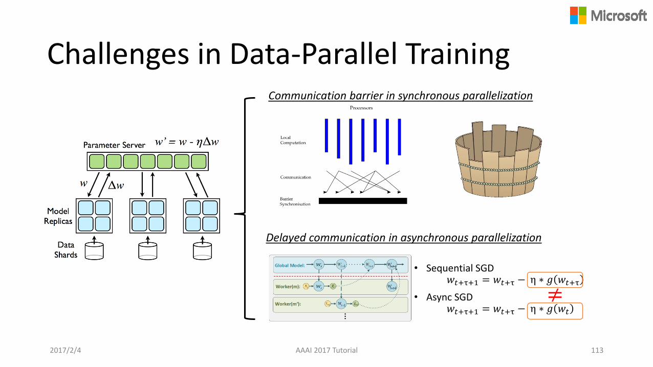
Challenges in Data-Parallel Training
• Sequential SGD𝑤𝑡+τ+1 = 𝑤𝑡+τ − η ∗ 𝑔 𝑤𝑡+τ
• Async SGD𝑤𝑡+τ+1 = 𝑤𝑡+τ − η ∗ 𝑔 𝑤𝑡
≠
Delayed communication in asynchronous parallelization
Communication barrier in synchronous parallelization
AAAI 2017 Tutorial 1132017/2/4
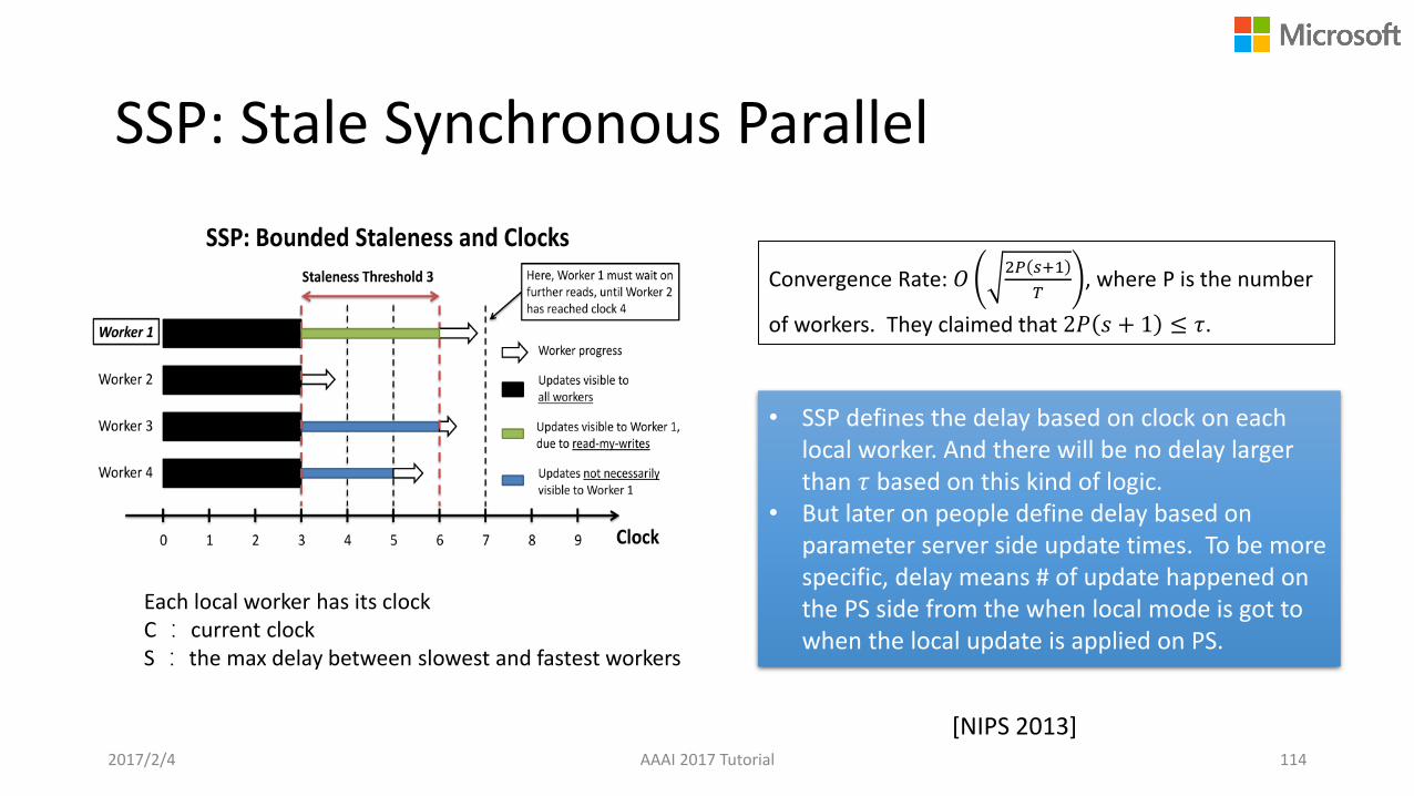
SSP: Stale Synchronous Parallel
Each local worker has its clockC : current clockS : the max delay between slowest and fastest workers
Convergence Rate: 𝑂2𝑃 𝑠+1
𝑇, where P is the number
of workers. They claimed that 2𝑃 𝑠 + 1 ≤ 𝜏.
• SSP defines the delay based on clock on each local worker. And there will be no delay larger than 𝜏 based on this kind of logic.
• But later on people define delay based on parameter server side update times. To be more specific, delay means # of update happened on the PS side from the when local mode is got to when the local update is applied on PS.
2017/2/4 AAAI 2017 Tutorial 114
[NIPS 2013]
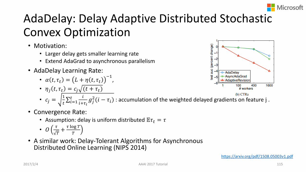
AdaDelay: Delay Adaptive Distributed Stochastic Convex Optimization• Motivation:
• Larger delay gets smaller learning rate• Extend AdaGrad to asynchronous parallelism
• AdaDelay Learning Rate:
• 𝛼 𝑡, 𝜏𝑡 = 𝐿 + 𝜂 𝑡, 𝜏𝑡−1
,
• 𝜂𝑗 𝑡, 𝜏𝑡 = 𝑐𝑗 (𝑡 + 𝜏𝑡)
• 𝑐𝑗 =1
𝑡σ𝑖=1𝑡 𝑖
𝑖+𝜏𝑖𝑔𝑗2(𝑖 − 𝜏𝑖) : accumulation of the weighted delayed gradients on feature j .
• Convergence Rate: • Assumption: delay is uniform distributed 𝔼𝜏𝑡 = 𝜏
• 𝑂𝜏
𝑇+
𝜏 log 𝑇
𝑇
• A similar work: Delay-Tolerant Algorithms for Asynchronous Distributed Online Learning (NIPS 2014)
https://arxiv.org/pdf/1508.05003v1.pdf
2017/2/4 AAAI 2017 Tutorial 115
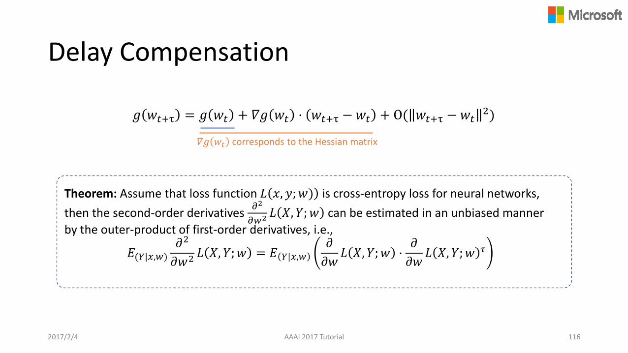
Delay Compensation
Theorem: Assume that loss function 𝐿 𝑥, 𝑦;𝑤) is cross-entropy loss for neural networks,
then the second-order derivatives 𝜕2
𝜕𝑤2 𝐿 𝑋, 𝑌;𝑤 can be estimated in an unbiased manner
by the outer-product of first-order derivatives, i.e.,
𝐸(𝑌|𝑥,𝑤)𝜕2
𝜕𝑤2𝐿 𝑋, 𝑌;𝑤 = 𝐸 𝑌|𝑥,𝑤
𝜕
𝜕𝑤𝐿 𝑋, 𝑌;𝑤 ⋅
𝜕
𝜕𝑤𝐿 𝑋, 𝑌;𝑤 𝜏
𝑔 𝑤𝑡+τ = 𝑔 𝑤𝑡 + 𝛻𝑔 𝑤𝑡 · 𝑤𝑡+τ −𝑤𝑡 + O( 𝑤𝑡+τ −𝑤𝑡2)
𝛻𝑔 𝑤𝑡 corresponds to the Hessian matrix
AAAI 2017 Tutorial 1162017/2/4
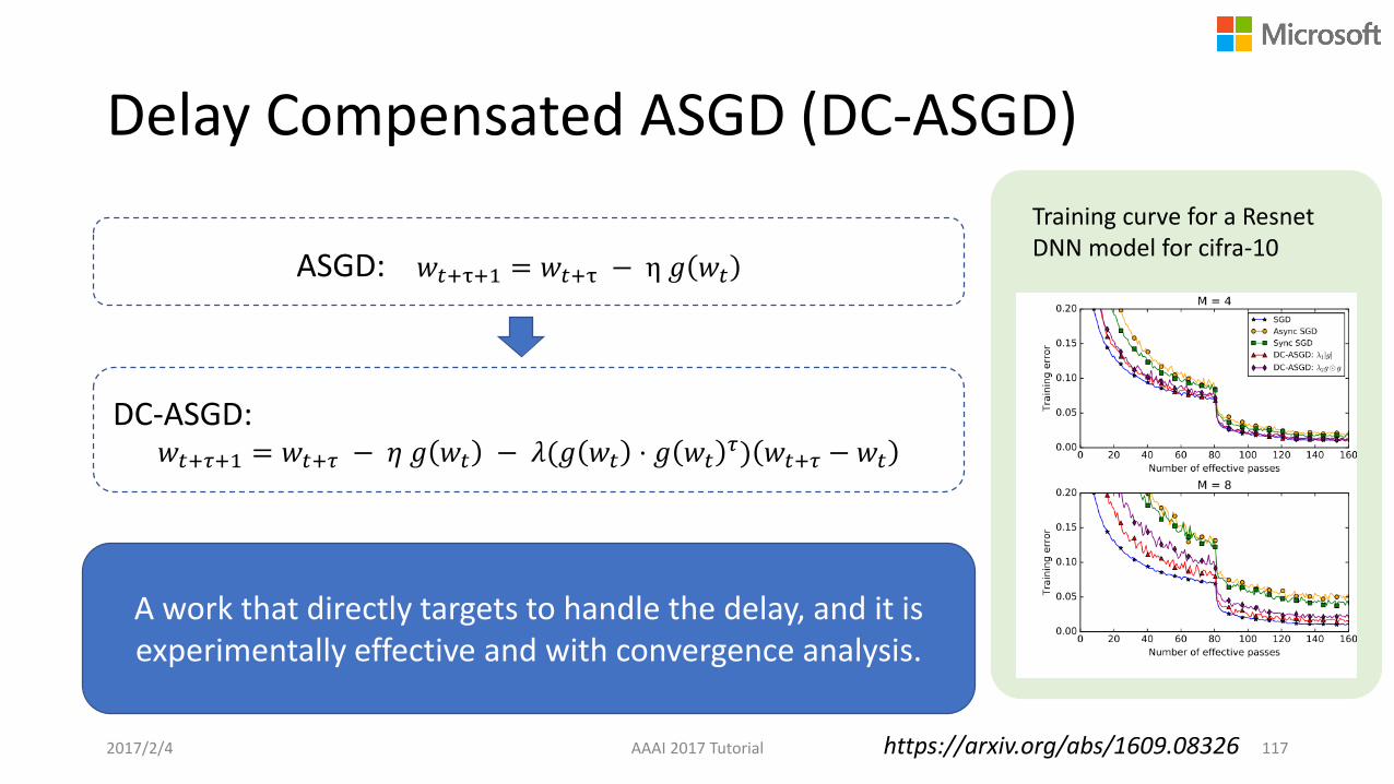
Delay Compensated ASGD (DC-ASGD)
AAAI 2017 Tutorial 117
ASGD: 𝑤𝑡+τ+1 = 𝑤𝑡+τ − η 𝑔 𝑤𝑡
DC-ASGD: 𝑤𝑡+𝜏+1 = 𝑤𝑡+𝜏 − 𝜂 𝑔 𝑤𝑡 − 𝜆(𝑔 𝑤𝑡 ⋅ 𝑔 𝑤𝑡
𝜏) 𝑤𝑡+𝜏 −𝑤𝑡
Training curve for a ResnetDNN model for cifra-10
A work that directly targets to handle the delay, and it is experimentally effective and with convergence analysis.
2017/2/4 https://arxiv.org/abs/1609.08326
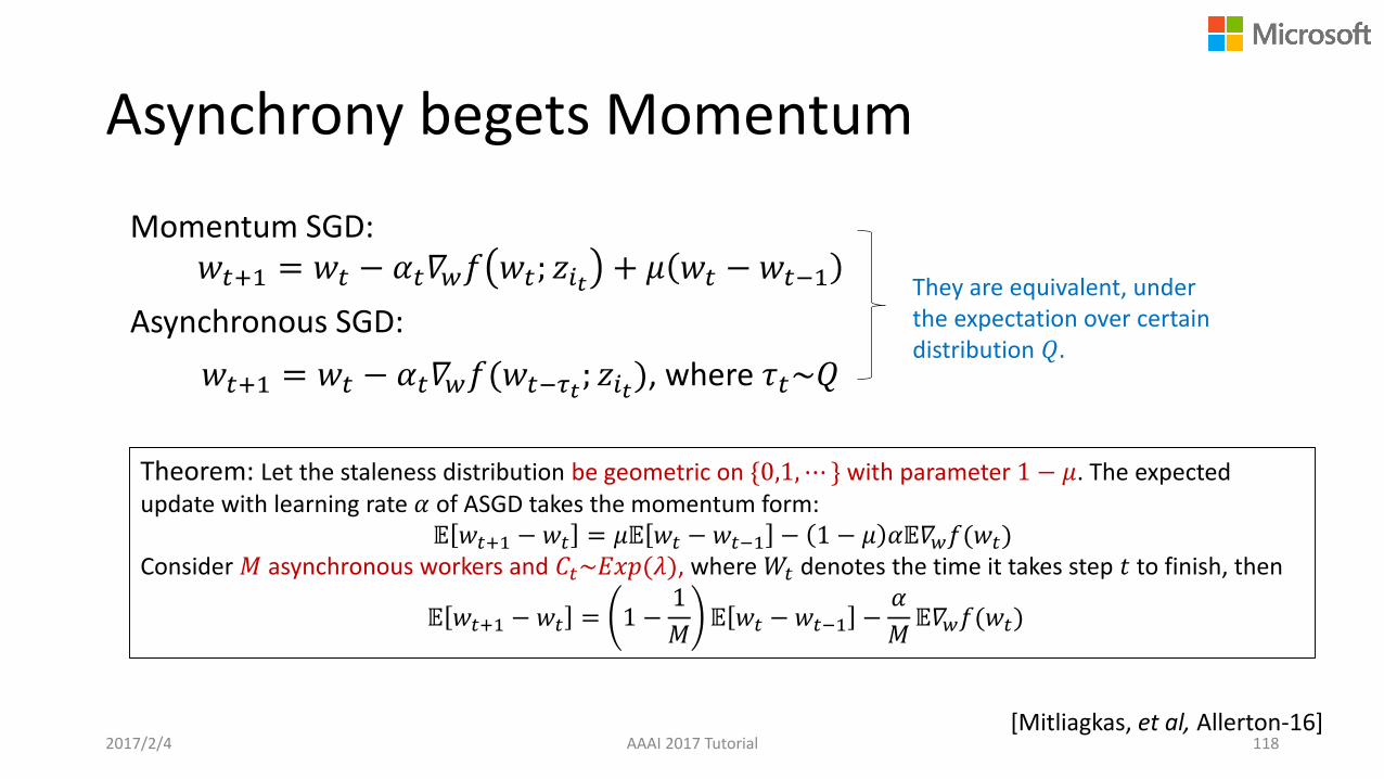
Asynchrony begets Momentum
Momentum SGD: 𝑤𝑡+1 = 𝑤𝑡 − 𝛼𝑡𝛻𝑤𝑓 𝑤𝑡; 𝑧𝑖𝑡 + 𝜇 𝑤𝑡 −𝑤𝑡−1
Asynchronous SGD:
𝑤𝑡+1 = 𝑤𝑡 − 𝛼𝑡𝛻𝑤𝑓(𝑤𝑡−𝜏𝑡; 𝑧𝑖𝑡), where 𝜏𝑡~𝑄
They are equivalent, under the expectation over certain distribution 𝑄.
Theorem: Let the staleness distribution be geometric on {0,1,⋯ } with parameter 1 − 𝜇. The expected update with learning rate 𝛼 of ASGD takes the momentum form:
𝔼 𝑤𝑡+1 − 𝑤𝑡 = 𝜇𝔼 𝑤𝑡 − 𝑤𝑡−1 − 1 − 𝜇 𝛼𝔼𝛻𝑤𝑓(𝑤𝑡)Consider 𝑀 asynchronous workers and 𝐶𝑡~𝐸𝑥𝑝(𝜆), where 𝑊𝑡 denotes the time it takes step 𝑡 to finish, then
𝔼 𝑤𝑡+1 − 𝑤𝑡 = 1 −1
𝑀𝔼 𝑤𝑡 −𝑤𝑡−1 −
𝛼
𝑀𝔼𝛻𝑤𝑓(𝑤𝑡)
[Mitliagkas, et al, Allerton-16]2017/2/4 AAAI 2017 Tutorial 118

Distribute ML Recent Advances
• Faster Stochastic Optimization Methods
• Non-convex Optimization
• Theoretical Analysis of Practical Data Allocation
• Handling Communication Delay
• Alternative Aggregation Methods
• Generalization Theory
2017/2/4 AAAI 2017 Tutorial 119
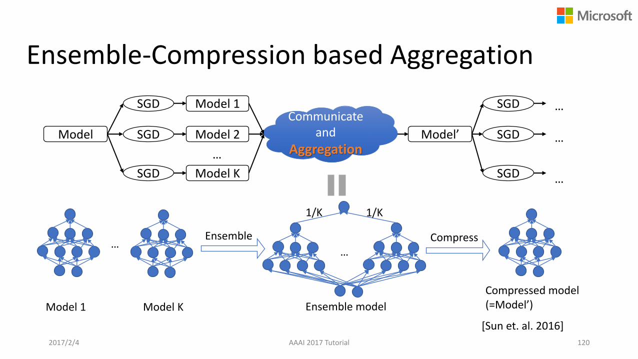
Ensemble-Compression based Aggregation
Communicate and
Aggregation
Model 1SGD
Model Model 2SGD
Model KSGD
…
SGD
Model’ SGD
SGD
…
…
…
…
Model 1 Model K
Ensemble
…
1/K 1/K
Compress
Compressed model (=Model’)Ensemble model
2017/2/4 AAAI 2017 Tutorial 120
[Sun et. al. 2016]
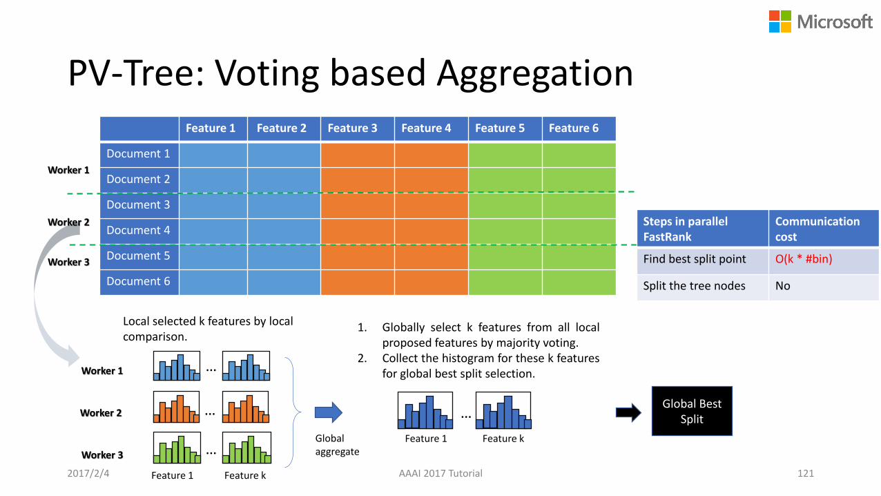
PV-Tree: Voting based AggregationFeature 1 Feature 2 Feature 3 Feature 4 Feature 5 Feature 6
Document 1
Document 2
Document 3
Document 4
Document 5
Document 6
Worker 1
Global Best Split
Local selected k features by local comparison.
Global aggregate
…
Feature 1 Feature k
…
…
…
Feature 1 Feature k
Worker 1
Worker 2
Worker 3
Worker 2
Worker 3
1. Globally select k features from all localproposed features by majority voting.
2. Collect the histogram for these k featuresfor global best split selection.
Steps in parallel FastRank
Communicationcost
Find best split point O(k * #bin)
Split the tree nodes No
2017/2/4 AAAI 2017 Tutorial 121
Distribute ML Recent Advances
• Faster Stochastic Optimization Methods
• Non-convex Optimization
• Theoretical Analysis of Practical Data Allocation
• Handling Communication Delay
• Alternative Aggregation Methods
• Generalization Theory
2017/2/4 AAAI 2017 Tutorial 122

Motivation
2017/2/4 AAAI 2017 Tutorial 123
Generalization Ability of Machine Learning Algorithms
min𝑓∈𝐹
𝑅 𝑓 =𝐸𝑍~𝑃𝑙(𝑓, 𝑍) min𝑓∈𝐹
𝑅𝑆 𝑓 =1
𝑛σ𝑖=1𝑛 𝑙(𝑓, 𝑍𝑖)
𝑃 is unknownNo closed-form solution
Optimization algorithm’s generalization error ?
Optimization algorithms: Convergence rate
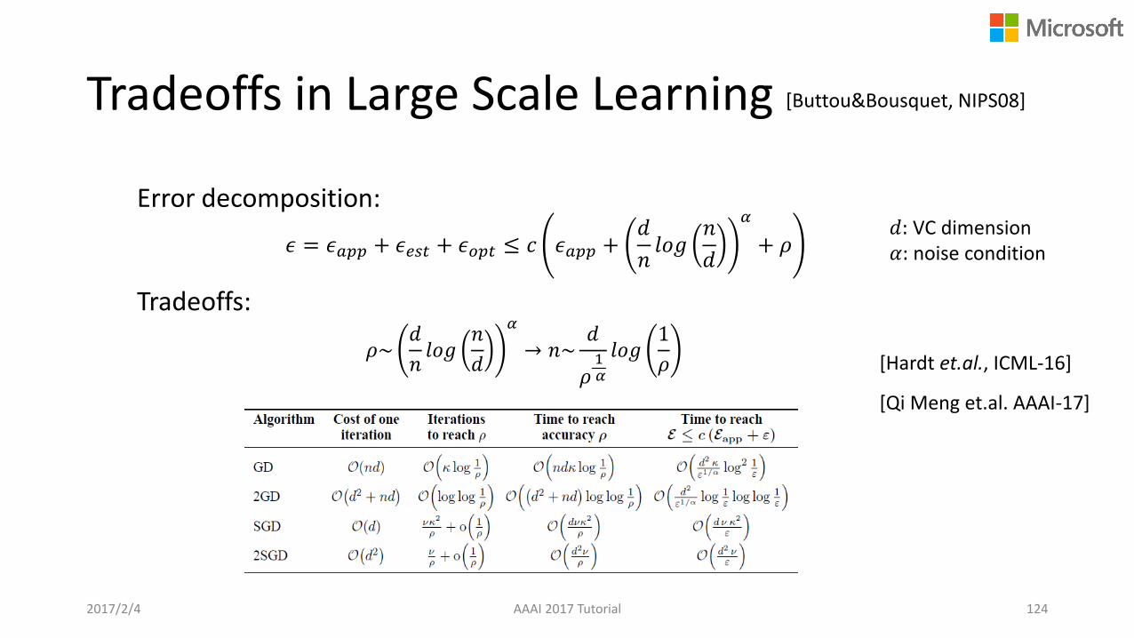
Tradeoffs in Large Scale Learning
Error decomposition:
𝜖 = 𝜖𝑎𝑝𝑝 + 𝜖𝑒𝑠𝑡 + 𝜖𝑜𝑝𝑡 ≤ 𝑐 𝜖𝑎𝑝𝑝 +𝑑
𝑛𝑙𝑜𝑔
𝑛
𝑑
𝛼
+ 𝜌
Tradeoffs:
𝜌~𝑑
𝑛𝑙𝑜𝑔
𝑛
𝑑
𝛼
→ 𝑛~𝑑
𝜌1𝛼
𝑙𝑜𝑔1
𝜌
[Buttou&Bousquet, NIPS08]
2017/2/4 AAAI 2017 Tutorial 124
[Hardt et.al., ICML-16]
[Qi Meng et.al. AAAI-17]
𝑑: VC dimension𝛼: noise condition

3. Distributed Machine Learning:Systems and Toolkits
2017/2/2 AAAI 2017 Tutorial 125

Distributed Machine Learning Architectures
AAAI 2017 Tutorial 126
Dataflow
Synchronous
Asynchronous
Data Parallelism Model Parallelism
Parameter Server
Irregular Parallelism
IterativeMapReduce • High-level abstractions (MapReduce)
• Lack of flexibility in modeling complex dependency
• Flexible in modeling dependency• Lack of good abstraction
• Support hybrid parallelism and fine-grained parallelization, particularly for deep learning
• Good balance between high-level abstraction and low-level flexibility in implementationTensorFlow
Petuum, DMLC
Spark
2017/2/2
Representative Systems and Toolkits
• Iterative MapReduce – Spark MLlib
• Parameter Server – DMTK
• Data Flow – TensorFlow
2017/2/2 AAAI 2017 Tutorial 127
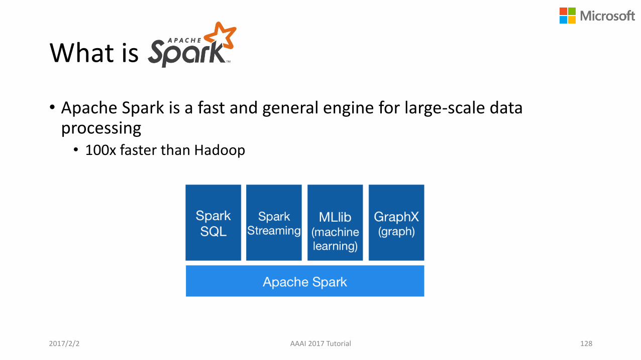
What is
• Apache Spark is a fast and general engine for large-scale data processing• 100x faster than Hadoop
2017/2/2 AAAI 2017 Tutorial 128
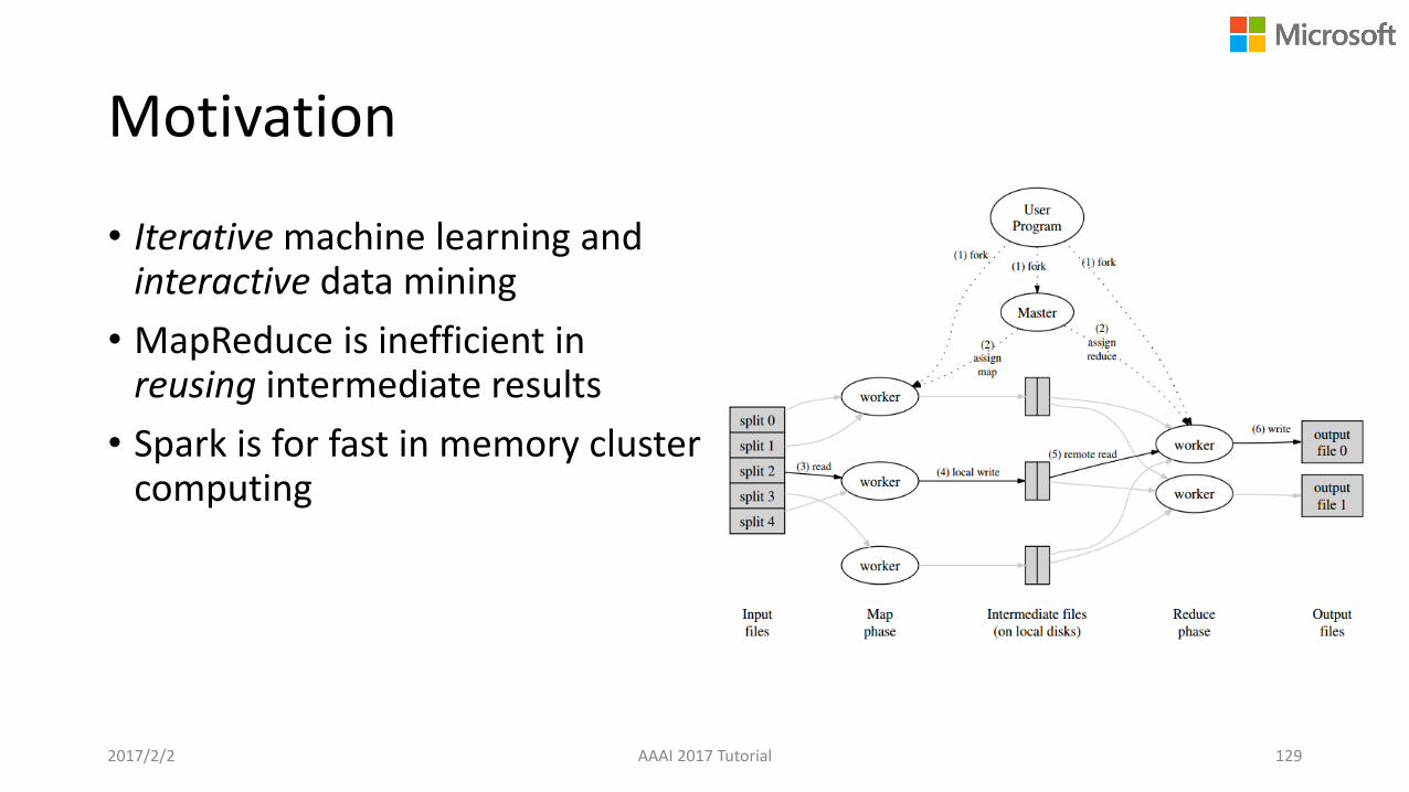
Motivation
• Iterative machine learning and interactive data mining
• MapReduce is inefficient in reusing intermediate results
• Spark is for fast in memory cluster computing
2017/2/2 AAAI 2017 Tutorial 129
Programming Model
• Resilient Distributed Datasets(RDDs)• Read-only, collection of distributed objects, can be rebuilt
• RDD Parallel Operations• Transformation and action on RDD
• map / filter / reduce / …
2017/2/2 AAAI 2017 Tutorial 130
MLLib
• Spark’s machine learning library
• Algorithms:• Classification: logistic regression, naïve Bayes
• Regression: generalized linear regression, isotonic regression
• Decision trees, random forests, and gradient-boosted trees
• Recommendation: alternating least squares(ALS)
• Clustering: K-means, Gaussian mixtures
• Topic modeling: latent Dirichlet allocation
2017/2/2 AAAI 2017 Tutorial 131
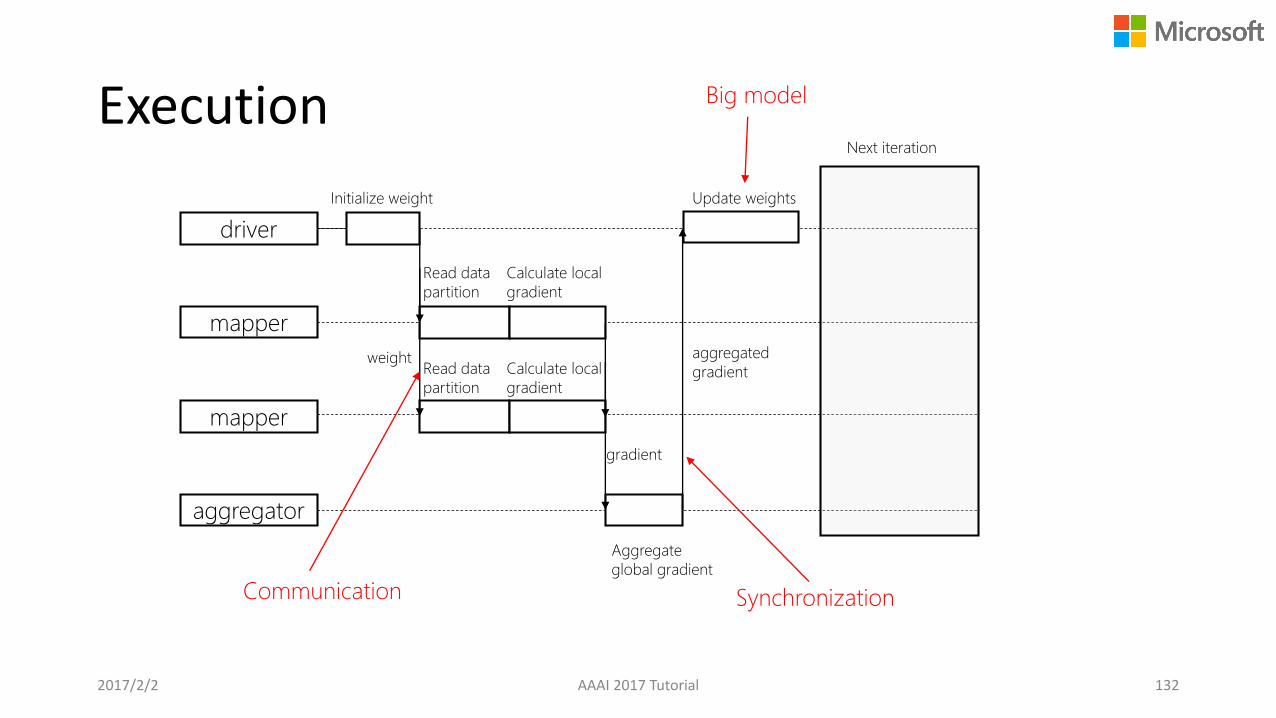
Execution
driver
mapper
mapper
aggregator
Initialize weight
Read data
partition
Calculate local
gradient
Read data
partition
Calculate local
gradient
weight
gradient
Aggregate
global gradient
aggregated
gradient
Update weights
Next iteration
Communication Synchronization
Big model
2017/2/2 AAAI 2017 Tutorial 132
Pros and Cons
• Pros• Simple interface and clean logic (MapReduce)
• High level programming language (Python, Scala, Java, SparkR)
• Convergence guarantee
• Cons• Not flexible enough for detailed optimization, e.g., pipelining
• Only support synchronous mode, might be very inefficient on large-scale heterogeneous cluster (when there are stragglers)
• Only support data parallelism, unclear how to support big models
2017/2/2 AAAI 2017 Tutorial 133
Representative Systems
• Iterative MapReduce - Spark
• Parameter Server – DMTK
• Data Flow – TensorFlow
2017/2/2 AAAI 2017 Tutorial 134

Parameter Server
• A specialized distributed key-value store for Machine Learning
• A group of servers managing shared parameters for a group of data-parallel workers
2017/2/2 AAAI 2017 Tutorial 135

Comparison with KV Store in DataBase
KV store DataBase Distributed ML
Data model Any data (Multi-d) (Sparse) array
Write access Write/Update/Append associative and commutative combiner
Consistency Strictly consistent ASP is accepted
Usage Highly available online service Offline data training
Replication Must have Typically no
Example Dynamo/Redis/Memcached Multiverso/PS/Petuum
2017/2/2 AAAI 2017 Tutorial 136
Parameter Server for Distributed ML
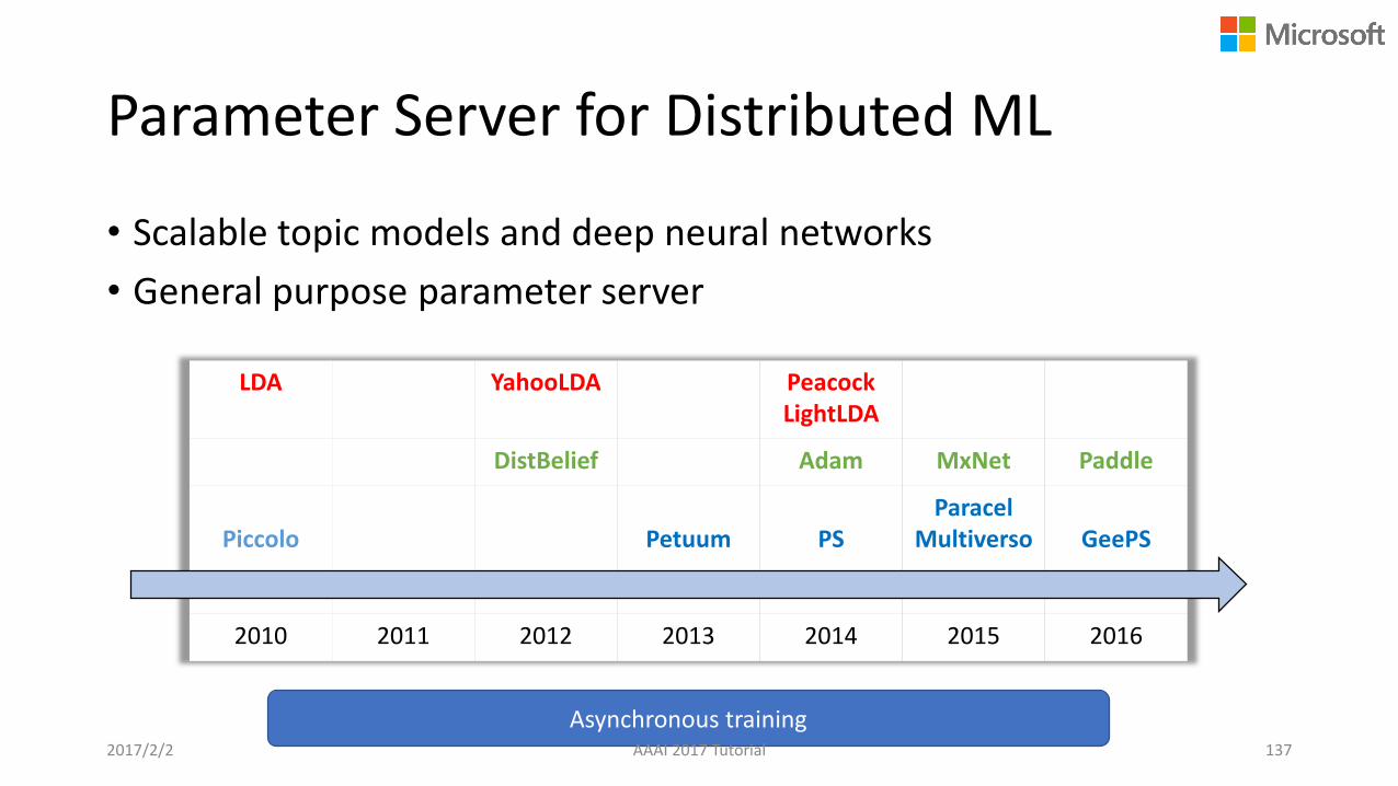
• Scalable topic models and deep neural networks
• General purpose parameter server
LDA YahooLDA PeacockLightLDA
DistBelief Adam MxNet Paddle
Piccolo Petuum PSParacel
Multiverso GeePS
2010 2011 2012 2013 2014 2015 2016
Asynchronous training2017/2/2 AAAI 2017 Tutorial 137
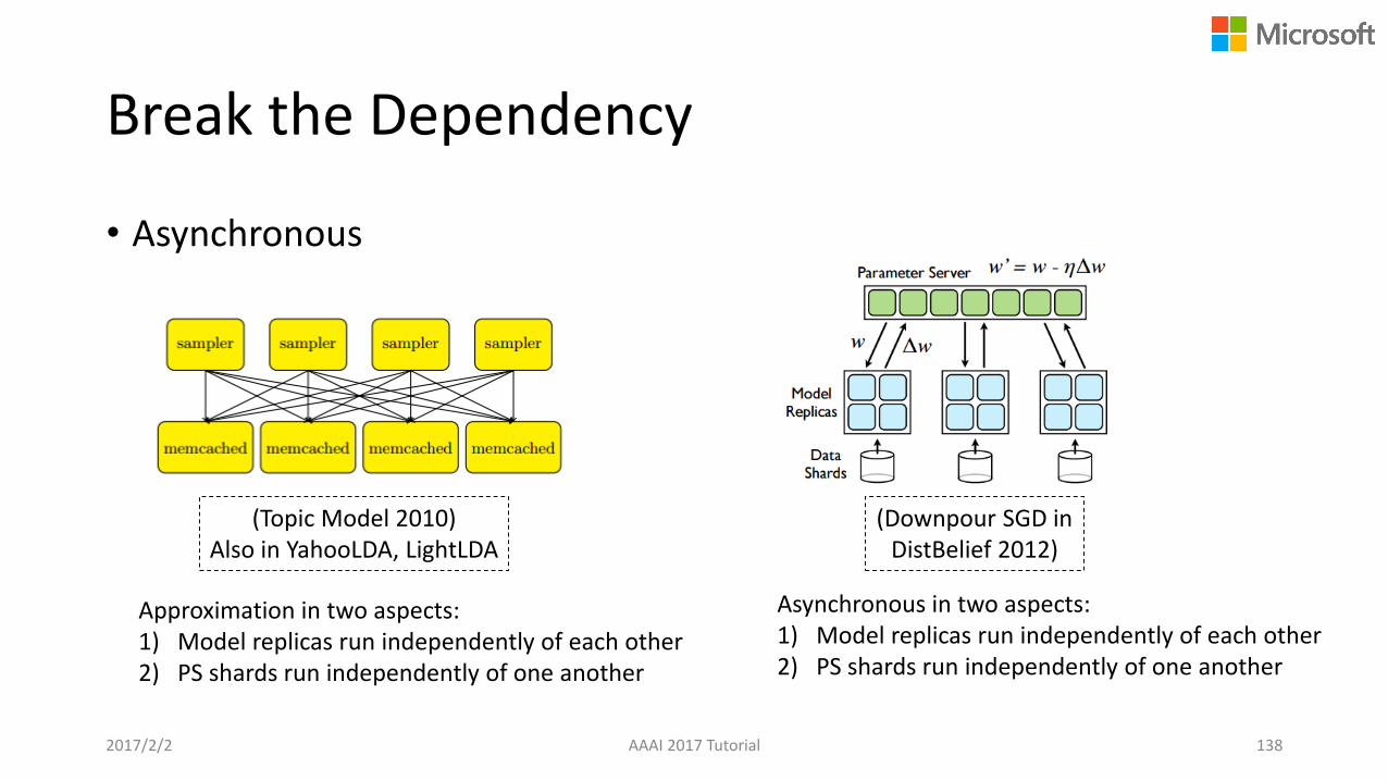
Break the Dependency
• Asynchronous
(Topic Model 2010)Also in YahooLDA, LightLDA
(Downpour SGD in DistBelief 2012)
Asynchronous in two aspects:1) Model replicas run independently of each other2) PS shards run independently of one another
Approximation in two aspects:1) Model replicas run independently of each other2) PS shards run independently of one another
2017/2/2 AAAI 2017 Tutorial 138

PS for DNN with GPU Cluster
• The mismatch in speed between GPU compute and network interconnects makes it extremely difficult to support data parallelism via a parameter server (ADAM 2014)
• GeePS• Big model – model swapping
• PS is still in CPU memory
2017/2/2 AAAI 2017 Tutorial 139
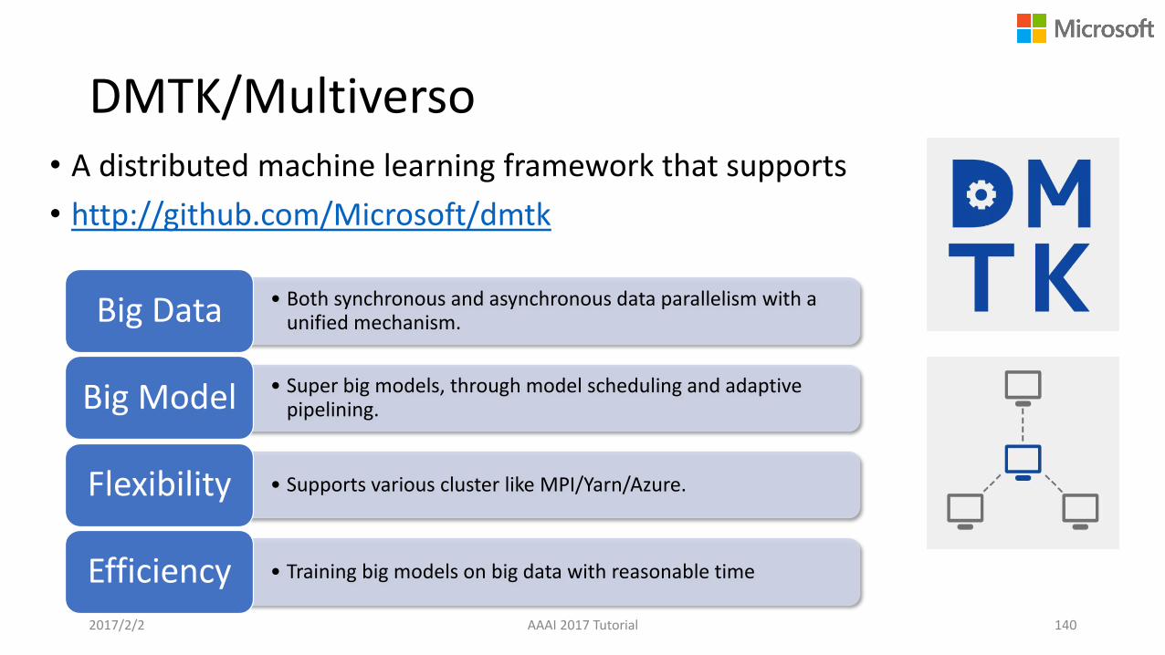
DMTK/Multiverso• A distributed machine learning framework that supports
• http://github.com/Microsoft/dmtk
• Both synchronous and asynchronous data parallelism with a unified mechanism.Big Data
• Super big models, through model scheduling and adaptive pipelining.Big Model
• Supports various cluster like MPI/Yarn/Azure.Flexibility
• Training big models on big data with reasonable timeEfficiency
2017/2/2 AAAI 2017 Tutorial 140

Unified Data Parallelism Interface
2017/2/2 AAAI 2017 Tutorial 141
Unified Interface:• Add(index 𝑖, delta Δ𝑊𝑖, coeff 𝑐):
• 𝑊(𝑡+1) = 𝑊(𝑡) + σ𝑖=1𝑛 𝑐 ⋅ Δ𝑊𝑖 ,
• 𝑐 = 1 for BSP/ASP/SSP;• 𝑐 = 1/𝑛 for MA/ADMM.
• SetDelay(delay):
• delay = 0: BSP, MA, ADMM;• delay > 0: SSP;• delay = ∞: ASP.
C++/C/python/Lua interfaces are supported, so that many algorithm lib users can benefit from using this tool. E.g. parallel Theano / Torch to work in multiple node scenario.
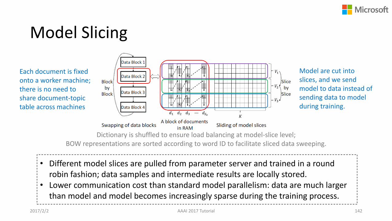
Model Slicing
142
• Different model slices are pulled from parameter server and trained in a round robin fashion; data samples and intermediate results are locally stored.
• Lower communication cost than standard model parallelism: data are much larger than model and model becomes increasingly sparse during the training process.
2017/2/2 AAAI 2017 Tutorial
Each document is fixed onto a worker machine; there is no need to share document-topic table across machines
Model are cut into slices, and we send model to data instead of sending data to model during training.
Dictionary is shuffled to ensure load balancing at model-slice level; BOW representations are sorted according to word ID to facilitate sliced data sweeping.

Communication Delay Allows Pipelining
Use pipelining to overlap data/model loading and computation.
2017/2/2 AAAI 2017 Tutorial 143
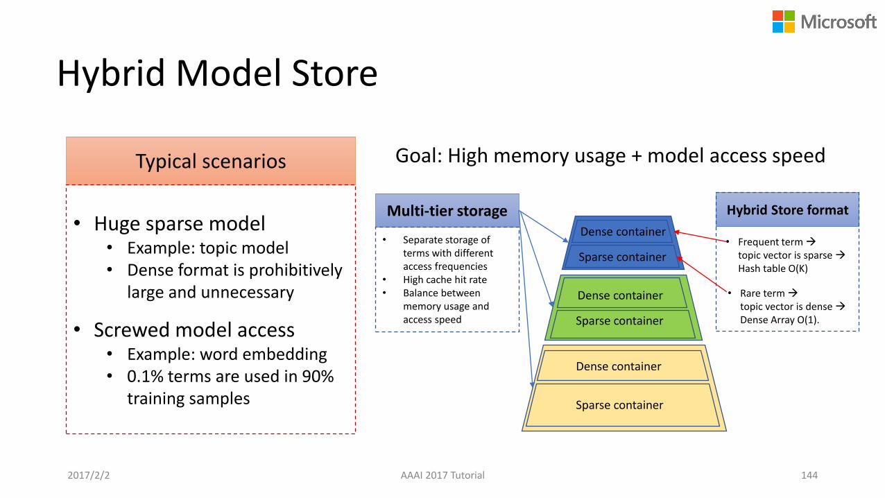
Typical scenarios
Hybrid Model Store
2017/2/2 AAAI 2017 Tutorial 144
• Huge sparse model• Example: topic model• Dense format is prohibitively
large and unnecessary
• Screwed model access• Example: word embedding• 0.1% terms are used in 90%
training samples
Goal: High memory usage + model access speed
Hybrid Store format
• Frequent term topic vector is sparse Hash table O(K)
• Rare term topic vector is dense Dense Array O(1).
Sparse container
Dense container
Sparse container
Dense container
Sparse container
Dense container
Multi-tier storage
• Separate storage of terms with different access frequencies
• High cache hit rate• Balance between
memory usage and access speed
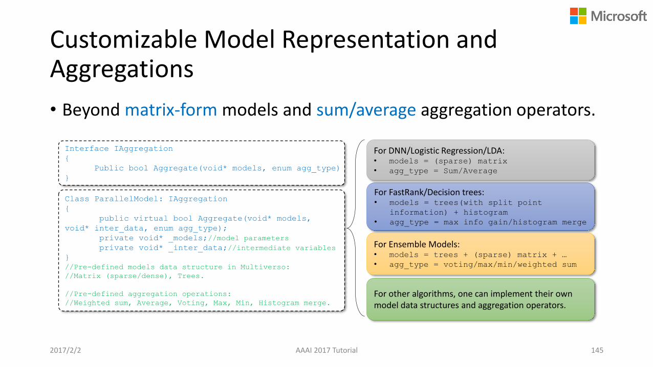
Customizable Model Representation and Aggregations
• Beyond matrix-form models and sum/average aggregation operators.
2017/2/2 AAAI 2017 Tutorial
Class ParallelModel: IAggregation
{
public virtual bool Aggregate(void* models,
void* inter_data, enum agg_type);
private void* _models;//model parameters
private void* _inter_data;//intermediate variables
}
//Pre-defined models data structure in Multiverso:
//Matrix (sparse/dense), Trees.
//Pre-defined aggregation operations:
//Weighted sum, Average, Voting, Max, Min, Histogram merge.
Interface IAggregation
{
Public bool Aggregate(void* models, enum agg_type)
}
For DNN/Logistic Regression/LDA: • models = (sparse) matrix
• agg_type = Sum/Average
For FastRank/Decision trees:• models = trees(with split point
information) + histogram
• agg_type = max info gain/histogram merge
For Ensemble Models: • models = trees + (sparse) matrix + …
• agg_type = voting/max/min/weighted sum
For other algorithms, one can implement their own model data structures and aggregation operators.
145
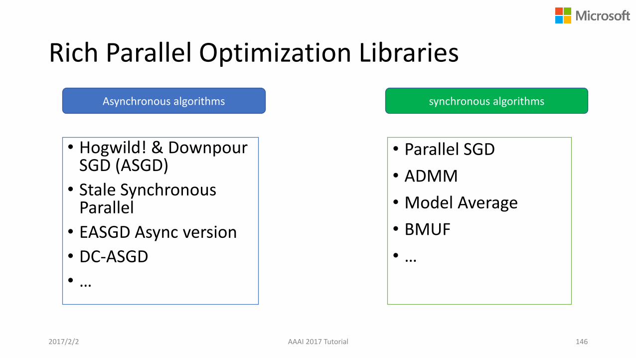
Rich Parallel Optimization Libraries
• Hogwild! & Downpour SGD (ASGD)
• Stale Synchronous Parallel
• EASGD Async version
• DC-ASGD
• …
• Parallel SGD
• ADMM
• Model Average
• BMUF
• …
Asynchronous algorithms synchronous algorithms
2017/2/2 AAAI 2017 Tutorial 146
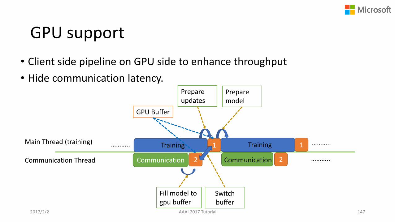
GPU support
• Client side pipeline on GPU side to enhance throughput
• Hide communication latency.
Main Thread (training)
Communication Thread
……….. Training 1 Training
Communication
1 ………..
………..
GPU Buffer
22Communication
Fill model to gpu buffer
Prepare updates
Prepare model
Switch buffer
2017/2/2 AAAI 2017 Tutorial 147
Representative Systems
• Iterative MapReduce - Spark
• Parameter Server – DMTK
• Data Flow – TensorFlow
2017/2/2 AAAI 2017 Tutorial 148
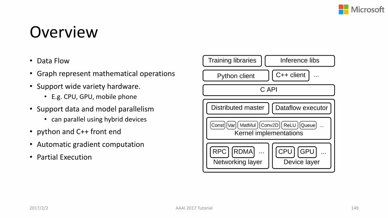
Overview
• Data Flow
• Graph represent mathematical operations
• Support wide variety hardware. • E.g. CPU, GPU, mobile phone
• Support data and model parallelism• can parallel using hybrid devices
• python and C++ front end
• Automatic gradient computation
• Partial Execution
2017/2/2 AAAI 2017 Tutorial 149
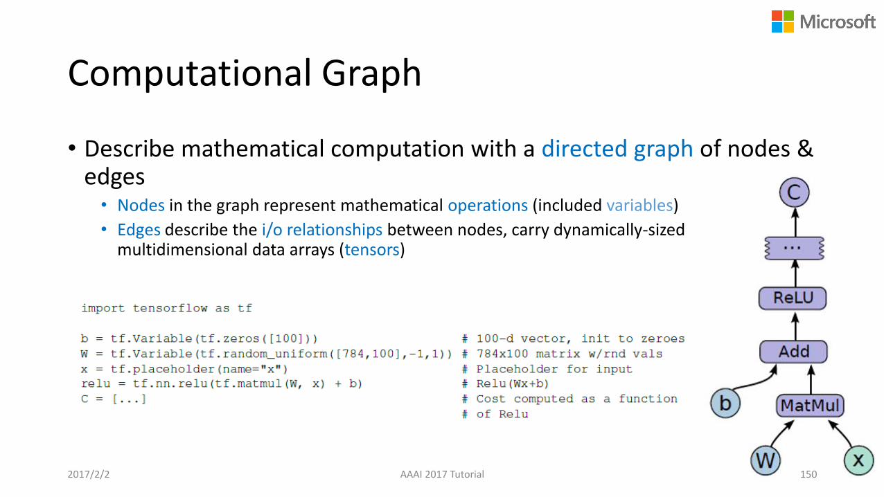
Computational Graph
• Describe mathematical computation with a directed graph of nodes & edges• Nodes in the graph represent mathematical operations (included variables)
• Edges describe the i/o relationships between nodes, carry dynamically-sized multidimensional data arrays (tensors)
2017/2/2 AAAI 2017 Tutorial 150
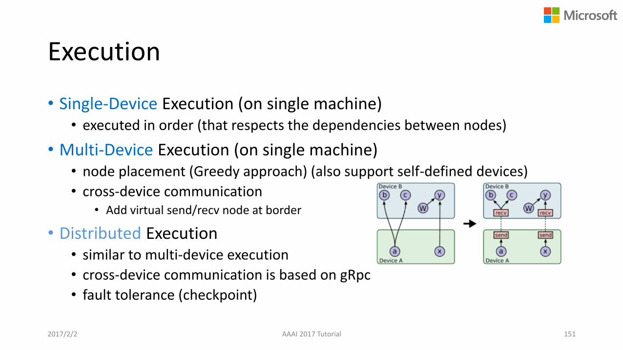
Execution
• Single-Device Execution (on single machine)• executed in order (that respects the dependencies between nodes)
• Multi-Device Execution (on single machine)• node placement (Greedy approach) (also support self-defined devices)
• cross-device communication• Add virtual send/recv node at border
• Distributed Execution• similar to multi-device execution
• cross-device communication is based on gRpc
• fault tolerance (checkpoint)
2017/2/2 AAAI 2017 Tutorial 151

Node Placement
• Run a simulated execution• Greedy heuristics
• Start with the sources of the graph
• For each node, choose the device where the node’s operation would finish the soonest (estimate by cost model)
• Cost model• Computation time
• Communication time
• But it seems this algorithm is not used in code base• “The placement algorithm is an area of ongoing development within the
system”2017/2/2 AAAI 2017 Tutorial 152
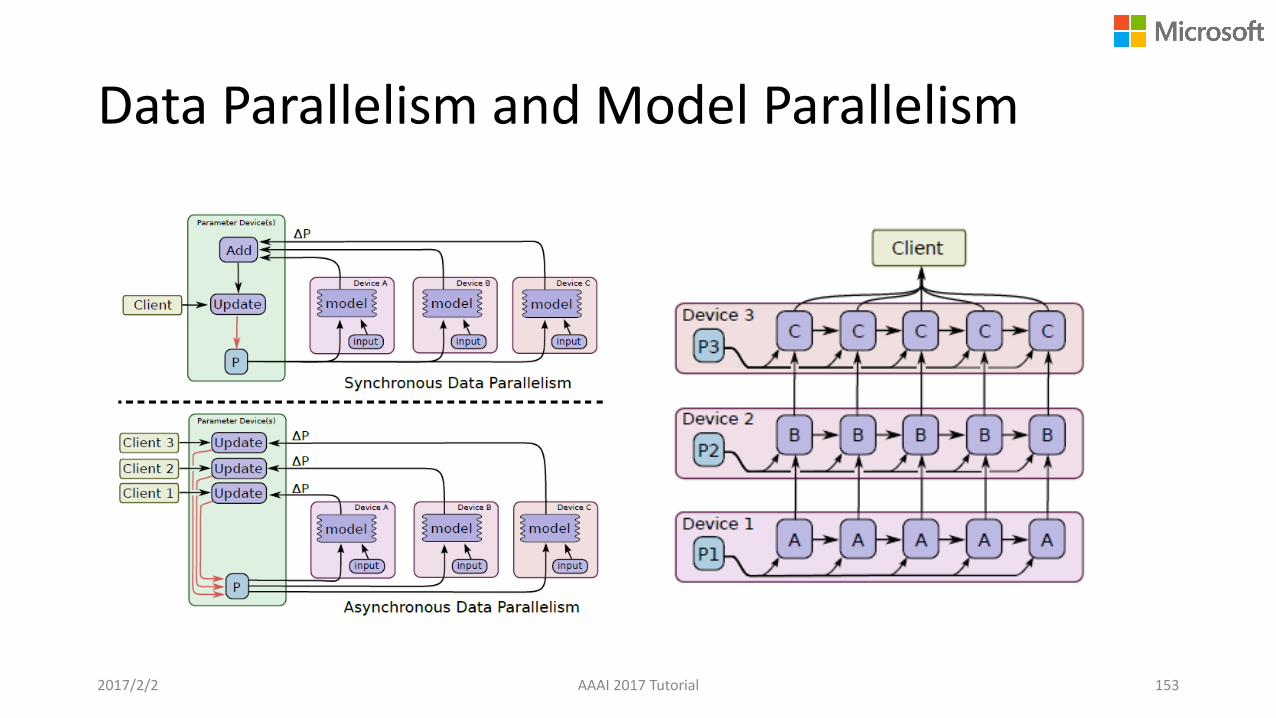
Data Parallelism and Model Parallelism
2017/2/2 AAAI 2017 Tutorial 153
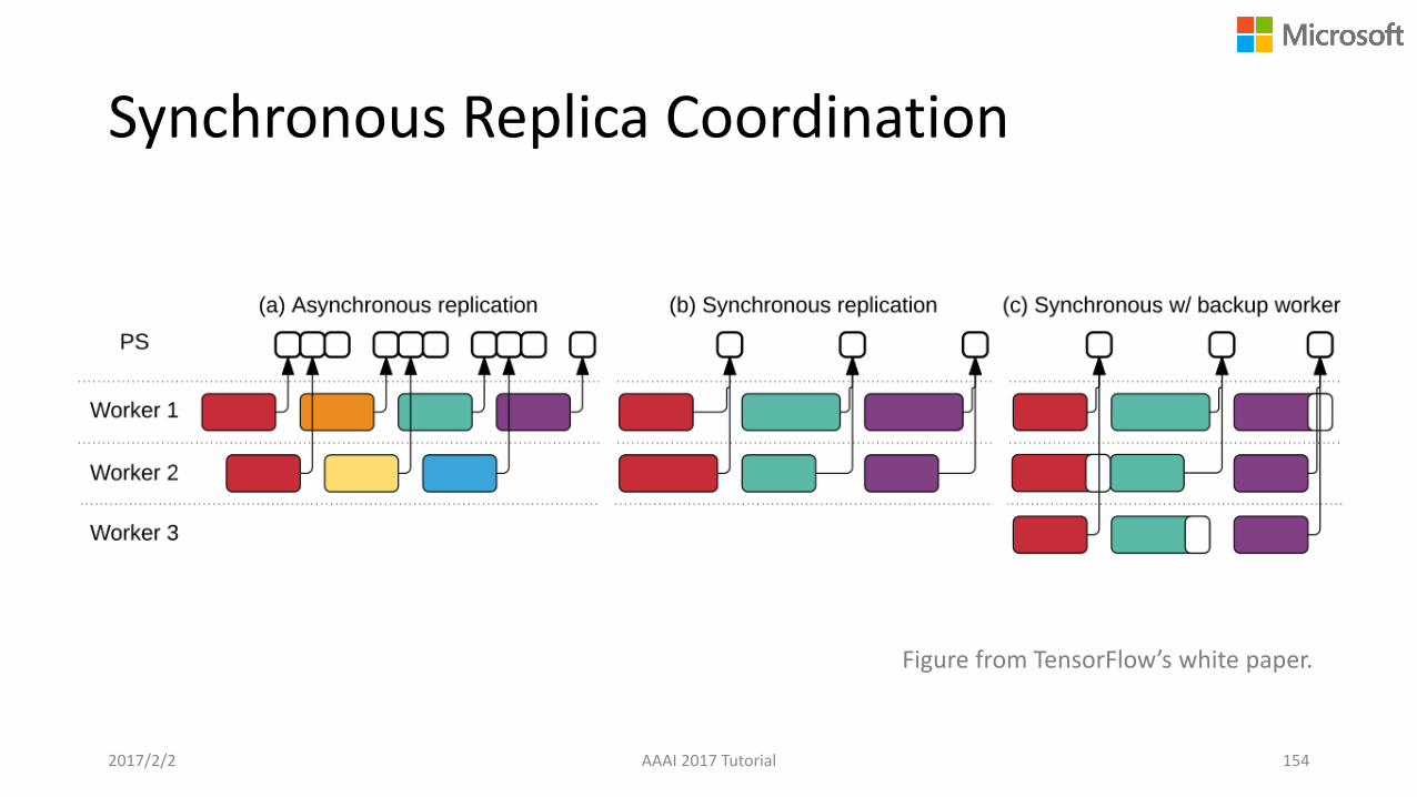
Synchronous Replica Coordination
Figure from TensorFlow’s white paper.
2017/2/2 AAAI 2017 Tutorial 154
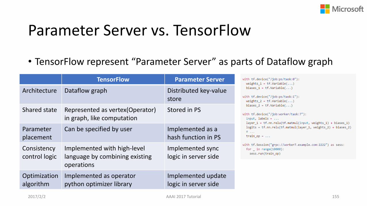
Parameter Server vs. TensorFlow
• TensorFlow represent “Parameter Server” as parts of Dataflow graph
TensorFlow Parameter Server
Architecture Dataflow graph Distributed key-value store
Shared state Represented as vertex(Operator)in graph, like computation
Stored in PS
Parameter placement
Can be specified by user Implemented as a hash function in PS
Consistencycontrol logic
Implemented with high-levellanguage by combining existing operations
Implemented sync logic in server side
Optimization algorithm
Implemented as operatorpython optimizer library
Implemented update logic in server side
2017/2/2 AAAI 2017 Tutorial 155
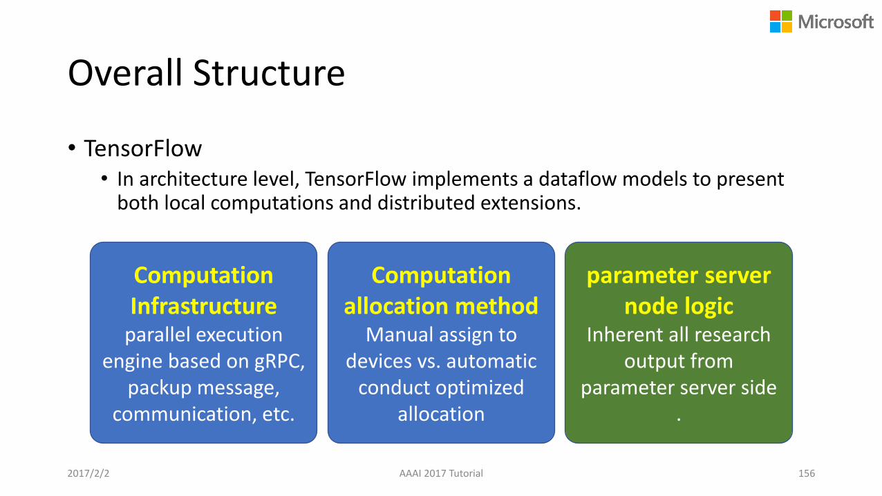
Overall Structure
• TensorFlow• In architecture level, TensorFlow implements a dataflow models to present
both local computations and distributed extensions.
Computation Infrastructure
parallel execution engine based on gRPC,
packup message, communication, etc.
Computation allocation method
Manual assign to devices vs. automatic
conduct optimized allocation
parameter server node logic
Inherent all research output from
parameter server side.
2017/2/2 AAAI 2017 Tutorial 156
Real Examples over Different Systems
• Machine learning systems• Spark MLlib
• DMTK - Parameter server
• TensorFlow
• Tasks• Logistic regression over three different systems
• DNN on DMTK+CNTK & TensorFlow (Resnet).
2017/2/2 AAAI 2017 Tutorial 157
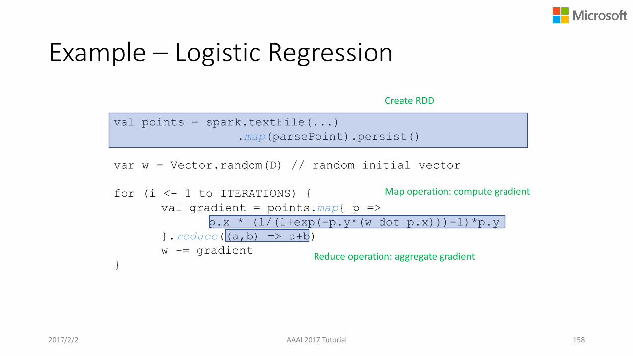
Example – Logistic Regression
val points = spark.textFile(...)
.map(parsePoint).persist()
var w = Vector.random(D) // random initial vector
for (i <- 1 to ITERATIONS) {
val gradient = points.map{ p =>
p.x * (1/(1+exp(-p.y*(w dot p.x)))-1)*p.y
}.reduce((a,b) => a+b)
w -= gradient
}
2017/2/2 158
Create RDD
Map operation: compute gradient
Reduce operation: aggregate gradient
AAAI 2017 Tutorial
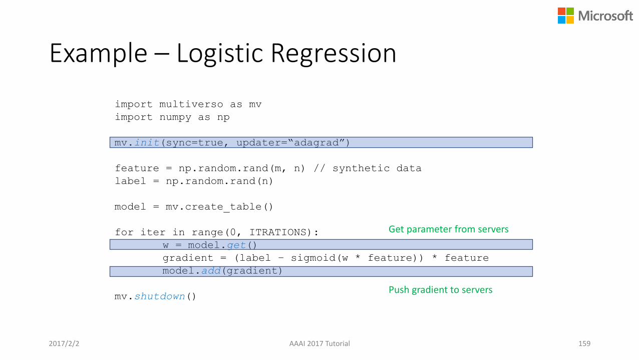
Example – Logistic Regression
import multiverso as mv
import numpy as np
mv.init(sync=true, updater=“adagrad”)
feature = np.random.rand(m, n) // synthetic data
label = np.random.rand(n)
model = mv.create_table()
for iter in range(0, ITRATIONS):
w = model.get()
gradient = (label – sigmoid(w * feature)) * feature
model.add(gradient)
mv.shutdown()
2017/2/2 159
Get parameter from servers
Push gradient to servers
AAAI 2017 Tutorial
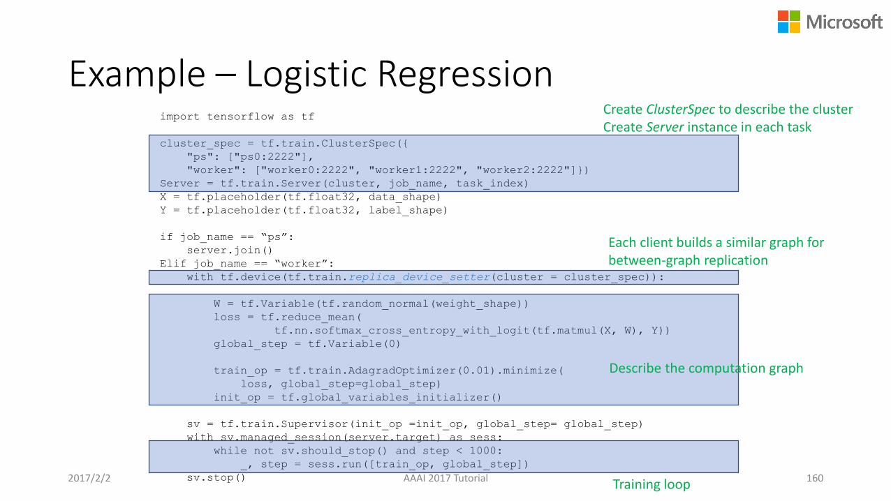
Example – Logistic Regressionimport tensorflow as tf
cluster_spec = tf.train.ClusterSpec({
"ps": ["ps0:2222"],
"worker": ["worker0:2222", "worker1:2222", "worker2:2222"]})
Server = tf.train.Server(cluster, job_name, task_index)
X = tf.placeholder(tf.float32, data_shape)
Y = tf.placeholder(tf.float32, label_shape)
if job_name == “ps”:
server.join()
Elif job_name == “worker”:
with tf.device(tf.train.replica_device_setter(cluster = cluster_spec)):
W = tf.Variable(tf.random_normal(weight_shape))
loss = tf.reduce_mean(
tf.nn.softmax_cross_entropy_with_logit(tf.matmul(X, W), Y))
global_step = tf.Variable(0)
train_op = tf.train.AdagradOptimizer(0.01).minimize(
loss, global_step=global_step)
init_op = tf.global_variables_initializer()
sv = tf.train.Supervisor(init_op =init_op, global_step= global_step)
with sv.managed_session(server.target) as sess:
while not sv.should_stop() and step < 1000:
_, step = sess.run([train_op, global_step])
sv.stop()2017/2/2 160
Create ClusterSpec to describe the cluster Create Server instance in each task
Describe the computation graph
Each client builds a similar graph for between-graph replication
Training loopAAAI 2017 Tutorial

Example – DMTK+CNTK on ResNet [K. He, et.al., 2016]
2017/2/2 AAAI 2017 Tutorial 161
Create model
Setting hyper-parameter
Create distributed learner for parallel training
Training loop
Test loop

Example – Tensorflow ResNet
2017/2/2 AAAI 2017 Tutorial 162
create server instance
create replica optimizer
Build model
Initialize queue and sessions
Training loop
Summary on Distributed Machine Learning Systems
• Flexibility and User Friendliness help the AI developers• Enclose all distributed algorithm details in high level abstractions to let user just use
distributed training• Expose simple but strong interface to advanced users to let them design their own
distributed algorithm
• Efficiency is key for solving big learning tasks• Leverage advanced hardware and software, e.g., GPU/RDMA • Use efficient sync up logic, e.g., Asynchronous algorithm + pipelining• Choose framework with less overhead cost, e.g., MapReduce v.s., parameter server
• Parallel Optimization method determine the accuracy• Apply advanced optimization algorithm in distributed training• SGD / SCD / Variance Reduction / Delay handling
2017/2/2 AAAI 2017 Tutorial 163