Pacific NorthwestNational Laboratory

Operated by Battelle for theU.S, Department of Energy

PNNL-12152 I

User’s Manual for CTCOOL:

A Computer Model for EvaluatingCombustion Turbine Inlet Air Cooling

S. KatipanmlaD.R. Brown

RECEIVED.JIjltlz8W9QSTI

May 1999

Prepared for the U.S. Department of Energy

under Contraci DE-AC06-76RL0 1830

DISCLAIMER

This report was prepared as an account of work sponsored by an agency ofthe United States Government. Neither the United States Government nor anyagency thereof, nor Battelle Memorial Institute, nor any of their employees,makes any warranty, express or implied, or assumes any legal liability orresponsibility for the accuracy, completeness, or usefulness of anyinformation,apparatus,product, or processdisclosed,or representsthat itsuse would not infringeprivatelyownedrights.Reference herein to any specificcommercial product, process, or service by trade name, trademark,manufacturer, or otherwise does not necessarily constitute or imply itsendorsement, recommendation, or favoring by the United States Governmentor any agency thereof, or Battelle Memorial Institute. The views and opinionsof authors expressed herein do not necessarily state or reflect those of theUnited States Government or any agency thereof.

PACIFIC NORTHWEST NATIONAL LABORATORYoperated by

BATTELLE MEMORIAL INSTITUTEfor the

UNITED STATES DEPARTMENT OF ENERGYunder Contract DE-AC06- 76RL0 1830

@ The contents of this report are printed on recycled paper.

-.

DISCLAIMER

Portions of this document may be illegiblein electronic image products. Images areproduced from the best available originaldocument.

PNNL-12152

user’s Manual for CTCOOL:A Computer Model for EvaluatingCombustion Turbine Inlet Air Cooling

S. KatipamulaD.R. Brown

May 1999

Prepared forThe U.S. Department of EnergyUnder Contract DE-AC06-76RL0 1830

Pacific Northwest National LaboratoryRichland, Washington 99352

~——.—— _.——. ~

I

I

I I

. .. ... . .

Summary

Combustion turbine generating capacity is inversely related to inlet air temperature. Conversely, peakgenerating demands, driven by space cooling needs, are positively related to ambient air temperature.Thus, generating capacity is low when the demand for electrici~ is the highest. Inlet air cooling offers aneffective method of increasing the generating capacity of combustion turbines.

Previously, the Pacific Northwest National Laboratory investigated several alternative inlet air cooling

systemsoverabroadrangeofapplicationconditions(Mown,Katipamul~andKonynenbelt1996).Theresults of this study showed that inlet air cooling was more cost-effective than building additionaluncooled combustion turbine power plants for all of the application conditions investigated. Thisincluded both aeroderivative and “industrial-frame” turbines in simple- and combined-cycleconfigurations. Cost-effectiveness was shown even for relatively, mild climates such as found in SanFrancisco.

A computer model called CTCOOL was developed to assist with the investigation described above.CTCOOL is a collection of C++ Classes developed under Microsoft Visual C-I+ 5.0@. The modelconsists of several input dialogs and analysis modules. In general, the model is capable of assessing theeconomic feasibility of cooling the inlet air to combustion turbines for site-specific conditions bysimulating the performance of the turbine, sizing necessary equipmen~ estimating the cost of theequipmen~ and calculating the monetary value of incremental power production and the net present valueof the capital investment.

This report describes CTCOOL and presents instructions for its use. For fi,uther itiorrnation amlor toreceive a copy of the CTCOOL sofhvare, please contact Srinivas Katipamula by email atSrinivas.Katipamula@,pnl.gov or by phone at (509) 372-4592.

...111

Contents

Summary ..................................................................................................................................................... 111 ....

1. Introduction .................................................................................................................................... ....... 1.

2. Inlet Air Cooling Overview ..................................................................................................................3

3. Model Overview ................................................................................................................................... 7

3.1. Model S~c~e ..............................................................................................................................".. 73.2. Model Capabilities ............................................................................................................................ 7

3.3. Model Limitations ............................................................................................................................. 8

4. Getting Started ...................................................................................................................................... 9

4.1. Hardware and Software Requirements .............................................................................................. 9

4.2. Installation In~ctions .........................................................................................................."..""..""..94.3. Starting CTCOOL ............................................................................................................................. 9

5. Input Screens ...................................................................................................................................... 11

5.1. Project Information Dialog ........................................................................................................".... 115.2. 1S0 Ratings Input Dialog .........................................................................................................."".... 125.3. Heat Rate Performance Coefficients Input Dialog .......................................................................... 13

5.4. Power Petiormance Coefficients Input Dialog ............................................................................... 145.5. Air Flow Rate Pefiorrnance Coefficients Input Dialog ................................................................... 155.6. Exhaust Flow Rate Petiormance Coefficients Input Dialog ........................................................... 16

5.7. Gas Turbine Operating Schedules Input Dialog ............................................................................. 175.8. Inlet Air Cooling Configuration Input Dialog ................................................................................. 185.9. Cooling Operating Schedule Input Dialog ...................................................................................... 18

5.10. Evaporative Cooling Input Dialog ................................................................................................ 19

5.11. Refrigerative Cooling Input Dialog ......................................................................................."""..."205.12. Aqua-Ammonia Chiller Performance Data Input Dialog ............................................................. 215.13. Complex-Compound Chiller Petiormance Data Input Dialog ...................................................... 225.14. Lithium Bromide Chiller Pefiormance Data Input Dialog ............................................................ 23

5.15. Vapor Compression Chiller Performance Data Input Dialog ....................................................... 245.16. RefHgerative Cooling Sizing Inputs Dialog .................................................................................. 255.17. Thermal Storage Configuration Input Dialog ............................................................................... 255.18. Evaporative Cooling Cost Inputs Dialog ...................................................................................... 265.19. Refrigerative Cooling Cost Input Dialog ...................................................................................... 27.

5.20. NPV Input Dialog ......................................................................................................................... 28

5.21. Input Summary Dialog .................................................................................................................. 29

5.22. Gas Turbine Petiormance Analysis Output Dialog ....................................................................... 29

5.23. Cooling Equipment Sizing Output Dialog .................................................................................... 30

5.24. Cooling Equipment Costs Output Dialog ..................................................................................... 305.25.NPV Calculations Results Dialog ......................................................................................."".."....-32

6. Sample Case ........................................................................................................................................ 33

6.1. Annual, Peak and Minimum Values for Selected pefiorm~ce p~eters .....”.....-”.””.”.-..”.....-.”.-..H6.2. Cooling Equipment Sizing Output ..................................................................................................

6.3. Cooling Equipment Cost Estimates ................................................................................................ 42

6.4. Net Present Value OuQuK ......................................................................................""....."....""...."."...43

7. Reference ................................................................................................................................... ......... 45

Appendix A Model Structure ...................................................................................................................A.l

Appendix B Custom Weather File Format ...............................................................................................B.2

Appendix C Component Sizing ...............................................................................................................C.1

C.I Chiller Sizing .............................................................................................................................c.l

v

.. —.. —

C.2 Storage Sizing...........................................................................................................................C.2

C.3 Inlet Air Cooling Coil Suing....................................................................................................C.2

C.4 Chilled Water Circulation SystemSizing.................................................................................. c.2

C.5 Ammonia Circulation SystemSuing ......................................................................................... c.3

C.6 Ice Generator Stiing .................................................................................................................C.4

C.7 Chilled Water Generator ..........................................................................................................C.4

C.8 CoolingTowerSizing................................................................................................................ C.4

C.9 Chiller ParcwiticEnergy ........................................................................................................... C.5

C.1O Heat Recove~ Steam Generators (HRSG) .....~....................................................................... C.5

C.1I Power Reduction Due to SteamExtraction ............................................................................. C.6

Appendix D Performance Analysis ..........................................................................................................D.1

D. I power Plmts ..............................................................................................................................D.I

D.2 ChilIers .....................................................................................................................~................D.4.

D.3 Storage....................................................................................................................................... D.7

D.4Fluid Circulation .......................................................................................................................D.8

D.5 Evaporative CooIing ..................................................................................................................D.8

D.6Auxiliary System Cooling ..........................................................................................................D.8

D.7 Turbine Met and Ekit Ekcess Pressure Drop ...........................................................................D.9

D.8 Combined-Cycle Steam Extraction Power Output Reduction ...................................................D.9

Appendix E Cost Analysis ....................................................................................................................... E.1

E.I ChiIIer Capital Costs .................................................................................................................E.1

E.2 Storage Capital Costs ...............................................................................................................E.2

E.3 InletAir Coil Capital Costs.......................................................................................................E.2

E.4 Fluid Circulation Capital Costs.................................................................................................E.2E.5 Miscellaneous Equipment Capital Costs....................................................................................E.3

E.6Annual Maintenance Costs ........................................................................................................E.4

vi

Figures

Figure 2.1 Typical Inlet Air Cooling Impacts on Combustion Turbine Performance .................................. 4Figure 2.2 Generic Inlet Air Cooling System ............................................................................................... 4Figure 5.1 CTCOOL Main Screen ............................................................................................................. 11Figure 5.2 Project Itiormation Dialog ....................................................................................................... 12Figure 5.3 1S0 Ratings Input Dialog .......................................................................................................... 13Figure 5.4 Heat Rate Performance Coefficients Input Dialog .................................................................... 14Figure 5.5 Power Performance Coefficients Input Dialog ......................................................................... 15Figure 5.6 Air Flow Rate Performance Coel%cients Input Dialog ............................................................. 16Figure 5.7 Exhaust Flow Performance Coefficients Input Dialog ............................................................. 17Figure 5.8 Gas Turbine Operating Schedules Input Dialog ....................................................................... 18Figure 5.9 Inlet Air Cotding Configuration Input Dialog .......................................................................... 18Figure 5.10 Cooling Operating Schedule Input Dialog .............................................................................. 19Figure 5.11 Evaporative Cooling Inputs Dialog ......................................................................................... 20Figure 5.12 Refrigerative Cooling Configuration Dialog .......................................................................... 21Figure 5.13 Aqua-Ammonia Chiller Pefiormance Data Input Dialog ....................................................... 22Figure 5.14 Complex-Compound Chiller Performance Data Input Dialog ................................................ 23Figure 5.15 Lithium Bromide Performance Data Input Dialog ......................................,...............0........... 24

Figure 5.16 Vapor Compression Chiller Petiorrnance Data Input Dialog ................................................. 24Figure 5.17 Refi-igerative Cooling Siziig Inputs Dialog ............................................................................ 25Figure 5.18 Thermal Storage Cor@uration Dialog ................................................................................... 26Figure 5.19 Evaporative Cooling Cost Inputs ............................................................................................ 26Figure 5.20 Refrigerative Cooling Cost Input Dialog ................................................................................ 27Figure 5.21 NPV Inputs Dialog .................................................................................................................. 28Figure 5.22 Echo of Inputs Dialog ............................................................................................................. 29Figure 5.23 Gas Turbine Pefiormance Analysis Output Dialog ................................................................. 30Figure 5.24 Cooling Equipment Sizing Calculations ................................................................................. 31Figure 5.25 Cooling Equipment Cost Estimates ........................................................................................ 31Figure 5.26 NPV Calculations Resul@....................................................................................................... 32Figure 6.1 Project Information ................................................................................................................... 33Figure 6.2 1S0 Rating for the Industrial Frame Gas Turbine ..................................................................... 34Figure 6.3 Heat Rate Performance Coefficients ......................................................................................... 34Figure 6.4 Power Performance Coefficient ............................................................................................... 35Figure 6.5 Air Flow Rate Petiormance Coefficients .................................................................................. 35Figure 6.6 Inlet Air Cooling Confi~ation ................................................................................................ 36Figure 6.7 Refrigerative Cooling Configuration ........................................................................................ 36Figure 6.8 Vapor Compression Performance Data ..................................................................................... 37

Figure 6.9 Re&igerative Cooling Sizing Inputs .......................................................................................... 37

Figure 6.10 Thermal Storage Cotil~ation ............................................................................................... 38Figure 6.11 Refiigerative Cooling Co* .................................................................................................... 39Figure 6.12 NPV Inpufi .............................................................................................................................. 40Figure A.1 Schematic of the CTCOOL Model Stictie ..........................................................................A.2

vii

--- .—.

Tables

Table B1 - Format for the Custom Weather File .......................................................................................B.lTable B2 – Sample Weather Data for Houston .........................................................................................B.lTable Cl - TI~ and U Values Used for Sizing Generator Cooling Coil..................................................c.2

...VII1

1. Introduction

Combustion turbine inlet air cooling (CTIAC) should be considered by the power generating industrywhen seeking attractive options for increasing peak generating capacity. Inlet air cooling increases thepower production capacity and decreases the heat rate of a combustion turbine during hot weather, whenthe demand for electricity is generally the greatest. Off-peak ice generation and storage using electrically-driven chillers has proven to be cost-effective under peak shaving conditions where there is a largedifference between the value of peak and off-peak power.

Previously,thePacificNorthwestNationalLaboratoryconductedanassessmentofCTIACoptionsforthe U.S. Department of Energy’s OffIce of Utility Technologies as part of its Thermal Energy StorageProgram. The principal objectives of this study were as follows:

1) Identi& the preferred CTIAC technology as a function of application conditions from currentlyavailable cooling technology

2)Identi& application conditions where currently available cooling technology is not cost-effective, i.e.,where construction of additional power plant capacity without CTIAC would be preferred

3) Determine the potential attractiveness of an advanced ammoniated salt solidlvapor absorption coolingsystem

4) Determine the potential attractiveness of cooling combustion turbine inlet air to O‘F (in addition tocooling inlet air to a temperature around 40 to 45 “F, which is considered standard practice for CTIAC.).

To address the objectives described above, a screening study was designed to evaluate the principalcooling system technology options over abroad range of application conditions. Application variablesincluded power plant type, power plant opemting schedule, cooling system operating schedule, designinlet air temperature, and climate. Cooling system technology options included evaporative orretilgerative cooling, refrigerative chiller type, the inclusion (or exclusion) of storage, and the type ofstorage (storage media type, daily or weekly cycle, and load-leveling or load-shifting design).

The results of this study were previously published in Brown, Katipamulz and Konynenbelt (1996). Thedocument that follows provides descriptive information and instructions for using the model developed byPNNL (CTCOOL) to evaluate the CTIAC options.

The following section provides an overview of inlet air cooling for those less fmiliar with the concept.The subsequent IWOsections introduce CTCOOL and provide instructions for getting the sofhvare set upand running on your computer. Detailed descriptions of the input screens and output options are providednext. The final chapter presents a sample case. Additional description of the model stmcture, underlyingequations, and weather file formatting requirements are presented in the appendices.

10perated for the U.S. Departmentof Energyby BattelleMemorialInstituteunderContractDE-AC06-76RL0 1830

1

-----

2. Inlet Air Cooling Overview

Combustion turbines are constant volume machines, i.e., air intake is limited to a fixed volume of airregardless of ambient air conditions. As air temperature rises, its density falls. Thus, although thevolumetric flow rate remains constant the mass flow rate is reduced as air temperature rises. Poweroutput is also reduced as air temperature rises because power output is proportional to mass flow rate.The conversion efficiency of the gas turbine also falls as air temperature rises because more power isrequired to compress the warmer air.

The impact of compressor inlet air temperature on mass flow rate, power outpu~ and conversionefficiency is shown in Figure 2.1 for a typical “industrial” type turbine. Per custom, conversion efficiencyis reported as a heat rate, which is the amount of fiel energy consumed per kwh of electricity produced.Thus, a rise in the heat rate is consistent with a drop in conversion eftlciency. In general, the relationshipsare linear with temperature, or nearly so.

The petiormance curves show the dramatic tiect of temperature on turbine performance, and theopportunity to improve performance via inlet afi cooling. Cooling the inlet air improves both the poweroutput and the heat rate, but the impact on power output is greater. Furthermore, the positive impacts onpower output and heat rate increase with higher ambient temperatures, when utilities typically experiencethe highest demand for power. Therefore, incremental power production is greatest at the time it is mostvalued. Usually, theprimary objective of gas turbine inlet air cooling is to increase peakpower output.The heat rate improvement is a signl~cant, but secondary benefit.

The relative importance of the two impacts depends mostly on the value of incremental kW and kwhproduction, the number of operating hours per year, and ambient air temperatures during the operatingperiod. A greater number of annual operating hours will increase the importance of the heat rate impactwhile fewer hours will emphasize the incretie in power output. Applications with a higher ratio ofaverage to peak ambient operating temperature will also increase the importance of the heat rate irnpac~all else equal.

In theory, power output could be fi.u-therincreased by cooling below the temperature range indicated inFigure 2.1. In practice, all turbines are designed around a maximum thrust level that sets a usefid limit onthe inlet air temperature. In particular, the maximum power output of “aeroderivative” lype turbines oftenoccurs around the freezing point and may actually decline below this temperature.

A block diagram of a generic combustion turbine inlet air cooling system, with and without storage, isshown in Figure 2.2. The basic building blocks are the chiller, its cooling tower, the air coil, andinterconnecting piping. Cold fluid from the chiller is pumped through the air coil, where the coolant isheated and returned to the chiller, while the inlet air is cooled prior to entering the compressor. The

cooling tower provides cooling water to the chiller condenser. Alternatively, an evaporative condensermight be used with some types of chillers. Including storage and its associated piping loop increases thenumber of system components, but allows the chiller and cooling tower components to be down-sized,.msuming that cooling is not conducted 24 hours per day. Storage also significantly reduces on-peakparasitic power consumption for electrically-driven chiller systems.

. —. —--

Heat Rate

Inlet AirMass Flow Rate

Power Output

o 10 20 30 40 50 60 70 80 90 100 110 120

Inlet Air Temperature,“F

Figure 2.1 Typical Inlet Air Coolbg Impacts on Combustion Turbine Performance

Air Coil Compressor Turbine

- ~-”DrlAmbient

Air

,----- -- -- ----- _____ _,Chilled :Water ;

,, v ,, -------------- Optional Equipment

: Storage**r I *

----- ----- .’Chilled Wateror Refrigerant

Chiller

CoolingWater

CoolingTower

Figure 2.2 Generic Inlet Air Cooling System

4

The fimdarnental benefits of inlet air cooling were described above. The most obvious cost is the up-frontinvestment and periodic maintenance of the inlet air cooling system hardware. The energy used to drivethe chiller may also result in a significant expense, although the cost will vary significantly depending onwhether the chiller is thermally or electrically-driven and whether the energy source is thermal or electric.Inclusion of an air cooling coil within the inlet duct to the compressor will incur an additional pressureloss, with negative consequences to power output and heat rate, but the impacts will generally be less than0.5’XO.

The previous two paragraphs described the use of refrigerative systems for cooling turbine inlet air. Acommonly employed alternative, besides not cooling the inlet air at all, is to use evaporative cooling.Direct contact evaporative cooling, accomplished bypassing the inlet air through a wetted medi~ can be

particularly effective in drier climates. Any consideration of refrigerative inlet air cooling should alsoconsider evaporative cooling as an option. Note that evaporative and refrigerative approaches should beconsidered independently. Evaporative cooling followed by refrigerative cooling would not reduce therefrigerative cooling load. It would only substitute latent load for sensible load.

5

. -----

3. ModelOverview

The combustion turbine inlet air cooling performance evaluation model is a collection of C++ Classesdeveloped under Microsoft Visual C+!- 5.0°.

3.1. Model Structure

The model consists of several input dialogs and several analysis modules. The key analysis modulesdetermine annual gas turbine performance, size coolingktorage equipment estimate the cost ofcoolingktorage equipmen~ and calculate the net present value of a given conflgumtion. Several TMY2weather files are provided with the soflsvare tool.

3.2. Model Capabilities

In general, the model is capable of assessing the economic feasibility of cooling the inlet air tocombustion turbines for site-specific conditions by simulating the petiormance of the turbine with inlet aircooling, sizing necessary components, calculating the cost of the components, and calculating themonetary value of the incremental power and the net present value (NW) of the investment. Sampleoutput from the model is presented in Section 6.

The model is capable of evaluating the performance of cooling the inlet air to turbines in simple-cycle(indus@ial frame and aeroderivative type) or combined-cycle plant configurations. The air to the turbinecan either be cooled relligeratively or evaporatively. Thermal energy storage is an option forrefi-iteratively cooled systems. The model allows either daily or weekly ice or water storage with load-shillhg or load-leveling storage designs. At the present time, the model can only handle three differentinlet air temperatures: 1) 52 “F, 2) 42 ‘F and 3) O‘F. For O‘F cooling, the model cools the air in lsvostages with two different chillers 1) from the ambient condition to 42 ‘F and 2) from 42 “F to O‘F. Thechillers can either be electrically-driven or thermally-activate~ for thermally-activated chillers, theturbine exhaust gas (simple-cycle) or steam Ilom the combined-cycle plant is used.

The performance analysis includes calculation of the power output and fuel consumption of thecombustion turbine, with and without inlet air cooling, and calculation of the parasitic powerconsumption of inlet air cooling system components. The latter includes compressor power for vaporcompression chillers, steam and pump power for absorption chillers, pump power for the various fluidcirculation systems, and fan power for the cooling tower.

The model is also capable of computing annual performance data with the ability to aggregateperformance calculated for each operating hour of the year, based on hourly weather data. Theperformance analysis is based on user-specified information that is described later in the report.

2The TypicalMeteorologicalYear (TNN) is a “@ical” year of weatherpreparedtiom a largedatabase of theSOLMETdata and is availablefor 239 stations in the U.S. The data includeone completeyear of hourlyvalues(8760values)for each of the followingparameters:direct (beam)solarradiation,total horizontalsolarradiation,dry-bulb(temperature),wet-bulb(temperature),dew-point(humidi~), wind speedand cloud cover. Thesedata areprovidedin a single file in ASCII format.The SOLMET(SOLarandMeteorological) hourly databasewas firstpreparedfor 26 cities that had measuredhourly solarradiationdata.Then it was extendedto 222 additionallocationsby usingmodels to generatesyntheticsolar radiationmeasuresforthese locations.

7

—..

3.3. Model Limitations

Although the model is a poweri%lanalysis tool, it has the following limitations:

1)

2)

3)

4)

The inlet air temperature is fixed to three values (52 ‘F, 42 ‘F and O‘F). ,

The storage media is limited to ice or water (the choice between ice and water is implicit i.e., if theair is cooled to 42 ‘F, ice storage is assumed; and for 52 ‘F, water storage is assumed).

In general, cooling in multiple stages is not possible. Currently, the model cools the air in a singlestage when the air is cooled to 42 ‘F or 52 ‘F, and in two stages when the air is cooled to O‘F.

The component sizing basis is limited to meeting 100% of the peak design con&tions.

4. Getting Started

4.1. Hardware and Softiare Requirements

The CTCOOL computer program was written for use on personal computers with an Intel 80486° orhigher processor running Windows 95@or Windows NT 4.0@or higher operating system. It also requiresa VGA or,better graphics monitor with at least 800x 600 resolution.

4.2. Installation Instructions

Installation consists of simply creating a unique directo~, preferably named “CTCOOL,” and thencopying all the files from the distribution diskettes into the newly created directory. The distributiondiskettes contain one executable file (ctcool.exe); the rest of the files are either typical meteorologicalyear (TMY) weather files (with extension *.wth) for various cities in the United States or the exampleinput files (with extensions *.ctc).

4.3. Starting CTCOOL

Once the executable file and the weather files are all copied into a user-created directory, the program canbe executed by double clicking the “ctcool.exe” file.

——.. — . .

. . ..

5. Input Screens

The inputs required to carry out the pefiormance analysis using CTCOOL are entered using the variousmenus shown in Figure 5.1. Although the menu-driven format allows the user to move easily throughoutthe program, most of the menu items are only activated by a previous menu selection. Therefore, the first

level menu hems on the main input screen are arranged in the order each should be defined. For example,the user must complete the inputs under the menu item “Project” before entering the inputs under theother menu items. However, the inputs can be changed at anytime before or after an analysis iscompleted.

In addition to other commands, the command to open an existing input file or to save an input file can befound under the “File” menu item. A brief description of each menu item is provided in the sections thatfollow.

Figure 5.1 CTCOOL Main Screen

5.1. Project Informatwn Dialog

The “Project Information” dialog (Figure 5.2) is the only item under the “Project” menu heading. Thisdialog allows file “labeling” with general project information and selection of the weather file. Thegeneral project information has no affect on the analysis; it only serves as an identifier. However, theselection of the weather file is critical to the analysis. Several weather files are provided with thesoftwar~ these files have been derived from the TMY weather tapes. The dialog provides the user theability to select a custom weather file by checking the “User Defined” button. After the “User Defined”button is checke~ the “Get File Name” button becomes active and the user can provide the path and the

11

—..—.—

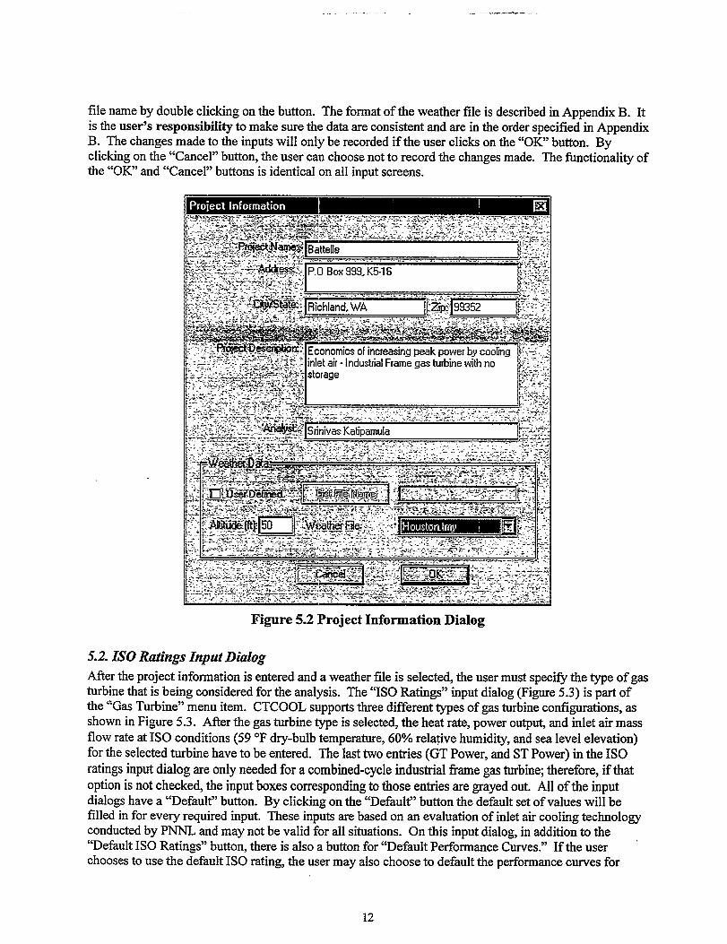
file name by double clicking on the button. The format of the weather file is described in Appendix B. Itis the user’s responsibility to make sure the data are consistent and are in the order specified in AppendixB. The changes made to the inputs will only be recorded if the user clicks on the “OK” button. Byclicking on the “Cancel” button, the user can choose not to record the changes made. The functionality ofthe “OK” and “Cancel” buttons is identical on all input screens.

Figure 5.2 Project Information Dialog

5.2. 1S0 Ratings Input Dialog

After the project information is entered and a weather file is selected, the user must speci~ the type of gasturbine that is being considered for the analysis. The “1S0 Ratings” input dialog (Figure 5.3) is part ofthe “Gas Turbine” menu item. CTCOOL supports three different types of gas turbine configurations, asshown in Figure 5.3. After the gas turbine type is selected, the heat rate, power output and inlet air massflow rate at 1S0 conditions (59 “F dry-bulb temperature, 60% relative humidity, and sea level elevation)for the selected turbine have to be entered. The last two entries (GT Power, and ST Power) in the 1S0ratings input dialog are only needed for a combined-cycle industrial fiarne gas turbine; therefore, if thatoption is not checked, the input boxes corresponding to those entries are grayed out. All of the inputdialogs have a “Default” button. By clicking on the “Default” button the default set of values will befilled in for every required input. These inpus are based on an evaluation of inlet air cooling technologyconducted by PNNL and may not be valid for all situations. On this input dialog, in addition to the“Default 1S0 Ratings” button, there is also a button for “Default Performance Curves.” If the user “chooses to use the default 1S0 rating, the user may also choose to default the performance curves for

12

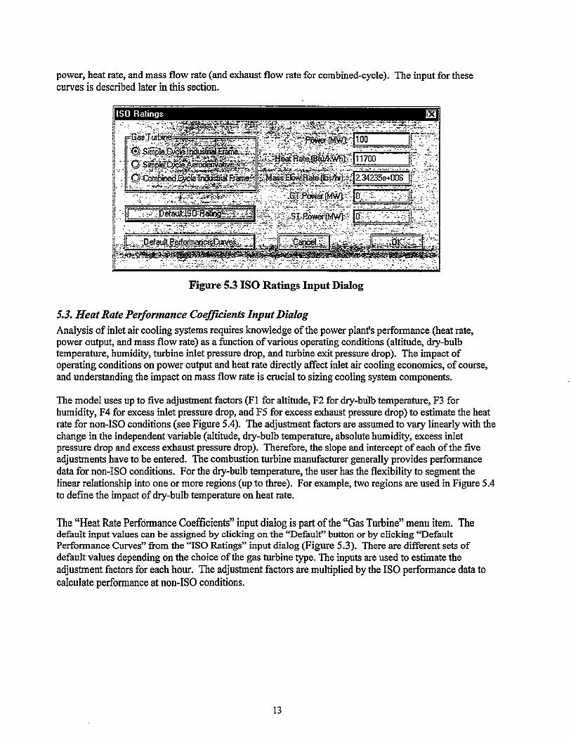
power, heat rate, and mass flow rate (and exhaust flow rate for combined-cycle). The input for thesecurves is described later in this section.

Figure 5.3 ISO Ratings Input Dialog

5.3. Heat Rate Performance Coefficients Input Dialog

Analysis of inlet air cooling systems requires knowledge of the power plant’s performance (heat rate,power outpu~ and mass flow rate) as a fimction of various operating conditions (altitude, dry-bulbtemperature, humidity, turbine inlet pressure drop, and turbine exit pressure drop). The impact ofoperating conditions on power output and heat rate directly tiect inlet air cooling economics, of course,and understanding the impact on mass flow rate is crucial to sizing cooling system components.

The model uses up to five adjustment factors (F1 for altitude, F2 for dry-bulb temperature, F3 forhumidity, F4 for excess inlet pressure drop, and F5 for excess exhaust pressure drop) to estimate the heatrate for non-ISO conditions (see Figure 5.4). The adjustment factors are assumed to vary linearly with thechange in the independent variable (altitude, dry-bulb temperature, absolute humidity, excess inletpressure drop and excess exhaust pressure drop). Therefore, the slope aud intercept of each of the fiveadjustments have to be entered. The combustion turbine manufacturer generally provides performancedata for non-ISO conditions. For the dry-bulb temperature, the user has the flexibility to segment thelinear relationship into one or more regions (up to three). For example, two regions are used in Figure 5.4to define the impact of dry-bulb temperature on heat rate.

The “Heat Rate Performance Coefi-lcients” input dialog is part of the “Gas Turbine” menu item. Thedefault input values can be assigned by clicking on the “Default” button or by clicking “DefaultPerformance Curves” from the “ISO Ratings” input dialog (Figure 5.3). There are different sets ofdefault values depending on the choice of the gas turbine lype. The inputs are used to estimate theadjustment factors for each hour. The adjustment factors are multiplied by the 1S0 performance data tocalculate performance at non-ISO conditions.

13

..—— —

Figure 5.4 Heat Rate Performance Coefficients Input Dialog

5.4. Power Performance Coefficients Input Dialog

Like the approach just described for modeling the heat rate, the model uses up to five adjustment factors

(FI foraltitude,F2fordry-bulbtemperature,F3forhumidity,F4forexcessinletpressuredrop,andF5for excess exhaust pressure drop) to estimate the power at non-ISO conditions (see Figure 5.5). Theadjustment factors are assumed to vary linearly with the change in the independent variable (altitude, dry-bulb temperature, absolute humidity, excess inlet pressure drop and excess exhaust pressure drop).Therefore, the slope and intercept of each of the five adjustments have to be entered. The combustionturbine manufacturer generally provides performance data for non-ISO conditions. For the dry-bulbtemperature, the user has the flexibility to segment the linear relationship into one or more regions (up tothree).

The “Power Pefiormance Coefficients” input dialog is part of the “Gas Turbine” menu item. The defaultinput values can be assigned by clicking on the “Default” button or by clickhg “Default PerformanceCurves” from the “1S0 Ratings” input dialog (Figure 5;3). There are different sets of default valuesdepending on the choice of the gas turbine type. The inputs are used to estimate the adjustment factorsfor each hour. The adjustment factors are multiplied by the 1S0 performance data to calculateperformance at non-ISO conditions.

14

—-. .— —

I

Figure 5.5 Power Performance Coefficients Input Dialog

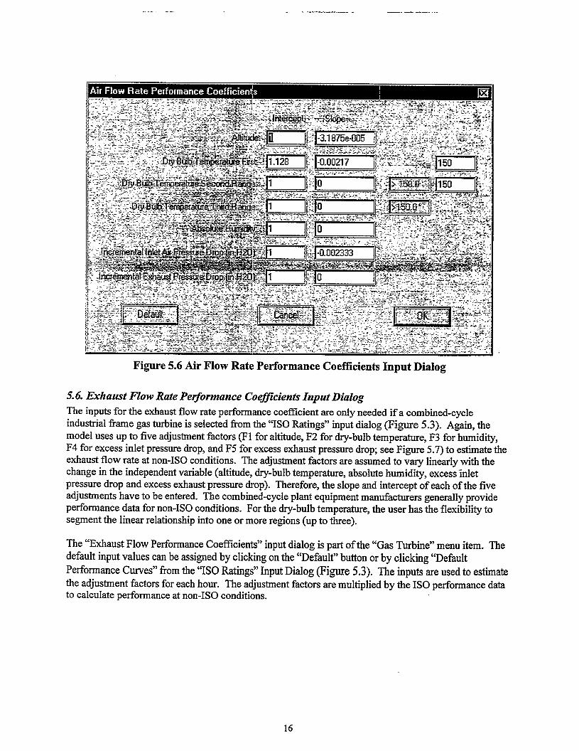
5.5. Air Flow Rate Performance Coefficien& Input Dialog

As for heat rate and power, the model uses up to five adjustment factors (F1 for altitude, F2 for dry-bulbtemperature, F3 for humidity, F4 for excess inlet pressure drop, and F5 for excess exhaust pressure drop)to estimate the air flow rate at non-ISO conditions (see Figure 5.6). The adjustment factors are assumedto vary linearly with the change in the independent variable (altitude, dry-bulb temperature, absolutehumidity, excess inlet pressure drop and excess exhaust pressure drop). Therefore, the slope and interceptof each of the five adjustments have to be entered. The combustion turbine manufacturer generallyprovides performance data for non-ISO conditions. For the dry-bulb temperature, the user has theflexibility to segment the linear relationship into one or more regions (up to three).

The “Air F1OWPerformance Coefficients” input dialog is part of the “Gas Turbine” menu item. Thedefault input values can be assigned by clicking on the “Default” button or by clicking “DefaultPefiormance Curves” from the “ISO Ratings” input dialog (Figure 5.3). T’heinputs are used to estimatethe adjustment factors for each hour. The adjustment factors are multiplied by the 1S0 performance datato calculate performance at non-ISO conditions.

15

.- ——- ..

Figure 5.6 Air F1OWRate Performance Coefficients Input Dialog

5.6. Exhaust Flow Rate Performance Coeff~ienfs Input Dialog

The inputs for the exhaust flow rate performance coefficient are only needed if a combined-cycleindustrial frame gas turbine is selected from the “ISO Ratings” input dialog (Figure 5.3). Again, themodel uses up to five adjustment factors (F1 for altitude, F2 for dry-bulb temperature, F3 for humidity,F4 for excess inlet pressure drop, and F5 for excess exhaust pressure drop; see Figure 5.7) to estimate theexhaust flow rate at non-ISO conditions. The adjustment factors are assumed to vary linearly with thechange in the independent variable (altitude, dry-bulb temperature, absolute humidity, excess inletpressure drop and excess exhaust pressure drop). Therefore, the slope and intercept of each of the fiveadjustments have to be entered. The combined-cycle plant equipment mantiacturers generally provideperl?ormancedata for non-ISO conditions. For the dry-bulb temperature, the user has the flexibility tosegment the linear relationship into one or more regions (up to three).

The “Exhaust Flow Performance Coefilcients” input dialog is part of the “Gas Turbine” menu item. Thedefault input values can be assigned by clicking on the “Default” button or by clicking “DefaultPerformance Curves” from the “ISO Ratings” Input Dialog (Figure 5.3). The inputs are used to estimatethe adjustment factors for each hour. The adjustment factors are multiplied by the 1S0 performance datato calculate performance at non-ISO conditions.

16

Figure 5.7 Exhaust Flow Performance Coefficients Input Dialog

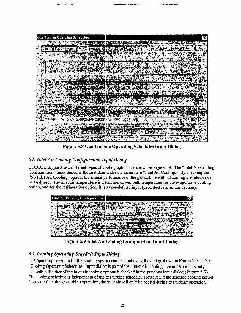
5.7. Gas Turbine Operating Schedules Input Dialog

The operating schedule for the gas turbine can be input using the dialog box shown in Figure 5.8. The“Gas Turbine Operating Schedules” input dialog is part of the “Gas Turbine” menu item. The user hasthe flexibility to speci~ when the gas turbine is started and stopped by the day-of-week and the month-of-year. For the inputs provided in Figure 5.8, the gas turbine will operate between 1400 hours and 1800hours (4 hours of operation) every day except Saturday and Sunday for the month of April. Similar inputscan be provided for the other months. To simpli~ inputs, additional buttons are provided at the bottom ofthe dialog. For example, the user can enter the schedule for 1 month and then copy the same schedule tothe other 11 months just by clicking on the “Copy” button (any previous values associated with the othermonths will be overwritten whh the values of the current month). Also, by simply clicking the “Clear”button, the schedule for any month can be cleared. Unlike the “Copy” button, the “C1ear” button onlyclears the current selection (month).

17

...—. .- —----- .—. .——

Figure 5.8 Gas Turbine Operating Schedules Input Dialog

5.8.Inlet Air Cooling ConfigurationInput Dialog

CTCOOL supports two different types of cooling options, as shown in Figure 5.9. The “Inlet Air CoolingConfiguration” input dialog is the first item under the menu item “Inlet Air Cooling.” By checking the“No Inlet Air Cooling” option, the annual pefiormance of the gas turbine without cooling the inlet air canbe analyzed. The inlet air temperature is a fimction of wet-bulb temperature for the evaporative coolingoption, and for the refiigerative option, it is a user-defined input (described later in this section).

Figure 5.9 Inlet Air Cooling Configuration Input Dialog

5.9. Cooling Operating Schedule Input Dialog

The operating schedule for the cooling system can be input using the dialog shown in Figure 5.10. The“Cooling Operating Schedules” input dialog is part of the “Inlet Air Cooling” menu item and is onlyaccessible if either of the inlet air cooling options is checked in the previous input dialog (Figure 5.9).The cooling schedule is independent of the gas turbine schedule. However, if the selected cooling periodis greater than the gas turbine operation, the inlet air will only be cooled during gas turbine operation.

18

The functionality of this input dialog is similar to the explanation provided for the gas turbine schedule(see Section 5.7)

Figure 5.10 Cooling Operating Schedule Input Dialog

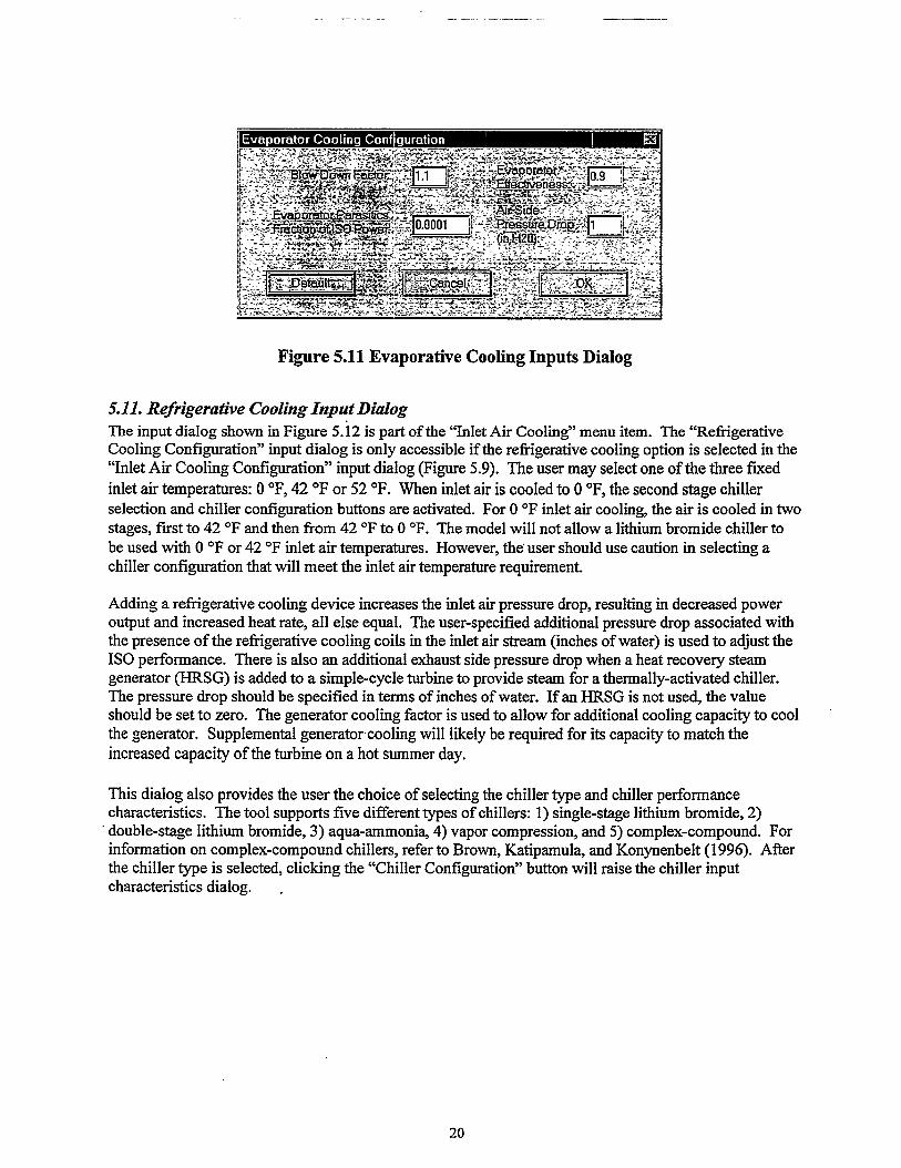
5.10. Evaporative Cooling Input Dtilog

The input dialog shown in Figure 5.11 is part of the “Inlet Air Cooling” menu item. The “EvaporatorCooling Configuration” input dialog is only accessible if the evaporative cooling option is selected in the“Inlet Air Cooling Conf@ration” input dialog (Figure 5.9). Only four inputs are required to simulate thepefiorrnance impacts with evaporative cooling. Although the water consumption for cooling airevaporatively is separately calculated, a user-specified input is used to calculate the additional water thatis consumed to accommodate blowdown requirements. The evaporator effectiveness is used to calculatethe temperature of the inlet air at the exit of the evaporator. The user may also specifi the parasitic powerrequirement of pumps, fans, etc., as a percent of the 1S0 power. Adding an evaporative cooling deviceincreases the inlet air pressure drop, resulting in decreased power output and increased heat rate, all elseequal. The user-specified additional pressure drop associated with the presence of the evaporator in theinlet air stream (inches of water) is used to adjust the 1S0 performance.

19

-- .— ___—.—__ . ——..

Figure 5.11 Evaporative Cooling Inputs Dialog

5.11. Refrigerative Cooling Input DialogThe input dialog shown in Figure 5.12 is part of the “Inlet Air Cooling” menu item. The “RefiigerativeCooling Configuration” input dialog is only accessible if the refrigerative cooling option is selected in the“Inlet Air Cooling Conf@ration” input dialog (Figure 5.9). The user may select one of the three f~edinlet air temperatures: O‘F, 42 ‘For 52 ‘F. When inlet air is cooled to O‘F, the second stage chillerselection and chiller configuration buttons are activated. For O‘F inlet air cooling, the air is cooled in twostages, first to 42 ‘F and then from 42 ‘F to O‘F. The model will not allow a lithium bromide chiller tobe used with O‘F or 42 “F inlet air temperatures. However, the-user should use caution in selecting achiller configuration that will meet the inlet air temperature requirement.

Adding a refrigerative cooling device increases the inlet air pressure drop, resulting in decreased poweroutput and increased heat rate, all else equal. The user-specified additional pressure drop associated withthe presence of the refrigerative cooling coils in the inlet air stream (inches of water) is used to adjust the1S0 petiormance. There is also an additional exhaust side pressure drop when a heat recovery steamgenerator (HRSG) is added to a simple-cycle turbine to provide steam for a thermally-activated chiller.The pressure drop should be specified in terms of inches of water. If an HRSG is not use& the valueshould be set to zero. The generator cooling factor is used to allow for additional cooling capacity to coolthe generator. Supplemental generator cooling will likely be required for its capacity to match theincreased capacity of the turbine on a hot summer day.

This dialog also provides the user the choice of selecting the chiller type and chiller petiormancecharacteristics. The tool supports five different lypes of chillers: 1) single-stage lithium bromide, 2)double-stage lithium bromide, 3) aqua-ammoni~ 4) vapor compression, and 5) complex-compound. Forinformation on complex-compound chillers, refer to Brown, Katipamul~ and Konynenbelt (1996). Afterthe chiller type is selected, clicking the “Chiller Configuration” button will raise the chiller inputcharacteristics dialog. .

20

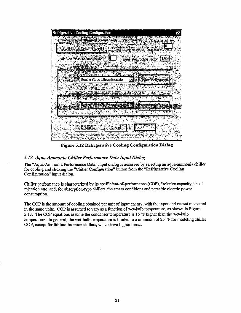
Figure 5.12 Refrigerative Cooling Configuration Dialog

5.12. Aqua-Ammonia Chiller Performance Data Input Dialog

The “Aqua-Ammonia Performance Data” input dialog is accessed by selecting an aqua-ammonia chillerfor cooling and clicking the “Chiller Configuration” button from the “Refrigerative CoolingConfiguration” input dialog.

Chiller pefiormance is characterized by its coefficient-of-performance (COP), “relative capacity,” heatrejection rate, and, for absorption-type chillers, the steam conditions and parasitic electric powerconsumption.

The COP is the amount of cooling obtained per unit of input energy, with the input and output measuredin the same units. COP is assumed to vary as a fimction of wet-bulb temperature, as shown in Figye5.13. The COP equations assume the condenser temperature is 15 ‘F higher than the wet-bulbtemperature. In general, the wet-bulb temperature is limited to a minimum of 25 “F for modeling chillerCOP, except for lithium bromide chillers, which have higher limits.

21

—.... -— .—- .—

Figure 5.13 Aqua-Ammonia Chiller Performance Data Input Dialog

Like the COP, the cooling capacity of a chiller is a function of the condenser temperature, and isexpressed here as a function of the wet-bulb temperature. The chiller cost equations presented later arebased on chiller capacity at “rated” temperature conditions. Capacity is typically less at temperatureconditions corresponding to the peak-cooling load. The “relative” capacity equation is applied to adjustthe peak chiller capacity to the rated chiller capacity.

All energy absorbed by a chiller at the evaporator and input to the chiller in the form of steam orelectricity must ultimately be rejected at a cooling tower. The heat rejection rate should be specified perton of cooling. The parasitic power input generally applies to the thermally-activated chillers only.

5.13. Coinplex-Compound Chiller Perfornuznce Data Input Dialog

The “Complex-Compound Chiller Pefiormance Data” input dialog (Figure 5.14) is accessed by selectinga complex-compound chiller for cooling and clicking the “Chiller Configuration” button from the“Refrigerative Cooling Configuration” dialog (Pigure 5.12).

The input requirements are similar to that of the aqua-ammonia chiller, with a second entry for heatrejection. The “storage” version of the complex-compo~d chiller is actially an integrated chiller-storagedevice that is sized based on ton-hours rather than tons. The first heat rejection rate is used to size heatrejection equipmen~ while the second heat rejection rate (the one associated with the storage option) isused to calculate the annual cooling load. Both the COP and the relative capacity are assumed to varylinearly as a fimction of the wet-bulb temperature.

22

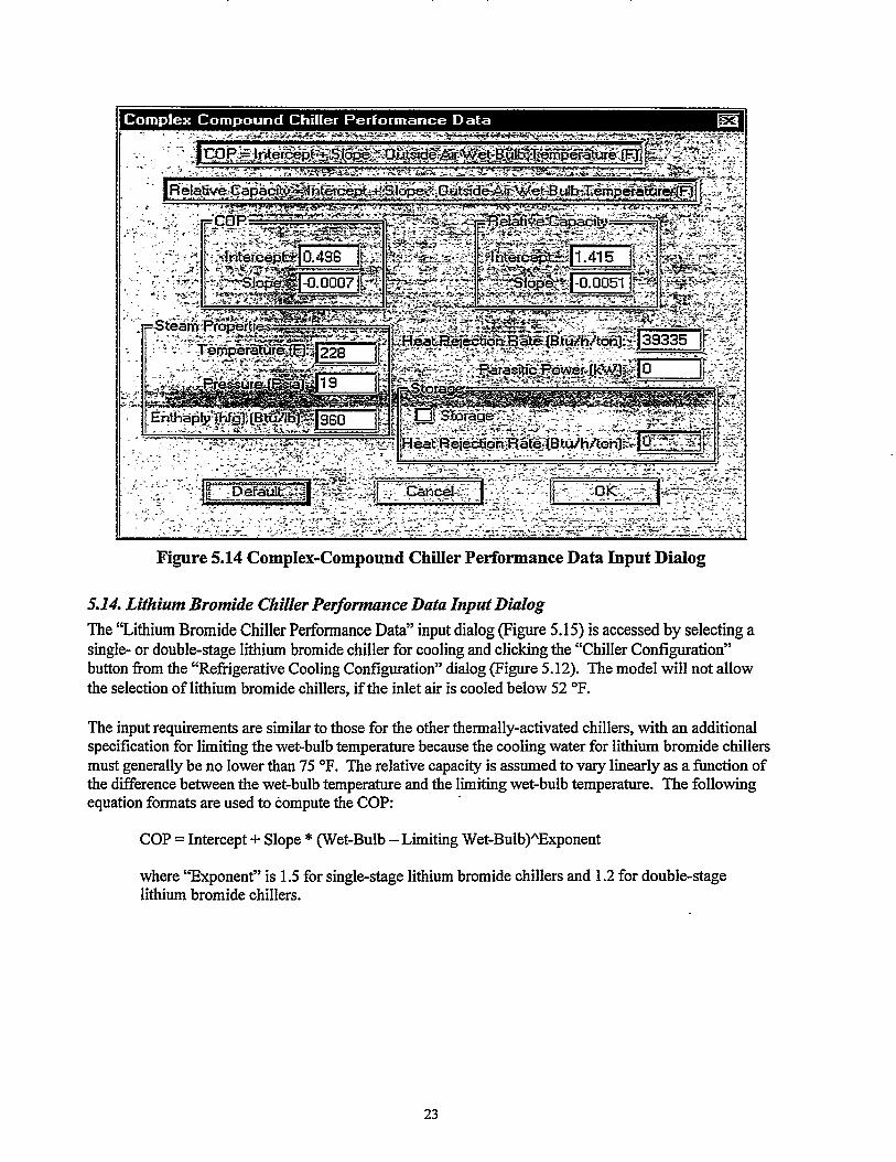
Figure 5.14 Complex-Compound Chiller Performance Data Input Dialog

5.14. Lithium Bromide Chiller Performance Data Input Dialog

The “Lithium Bromide Chiller Performance Data” input dialog (Figure 5.15) is accessed by selecting asingle- or double-stage lithium bromide chiller for cooling and clicking the “Chiller Configuration”button from the “Refrigerative Cooling Configuration” dialog (Figure 5.12). The model will not allowthe selection of lithium bromide chillers, if the inlet air is cooled below 52 “F.

The input requirements are similar to those for the other thermally-activated chillers, with an additionalspecification for limiting the wet-bulb temperature because the cooling water for lithium bromide chillersmust generally be no lower than 75 “F. The relative capacity is assumed to vary linearly as a fimction ofthe difference between the wet-bulb temperature and the limiting wet-bulb temperature. The followingequation formats are used to compute the COP:

COP = Intercept+ Slope* (Wet-Bulb – Limiting Wet-Bulb)’Exponent

where “Exponent” is 1.5 for single-stage lithium bromide chillers and 1.2 for double-stagelithium bromide chillers.

23

. ....—.

Figure 5.15 Lithium Bromide Performance Data Input Dialog

5.15. Vapor Compresswn Chiller Performance Data InpntDialog

The “Vapor Compression Performance Data” input dialog (Figure 5.16) is accessed by selecting a vaporcompression chiller for cooling and clicking the “Chiller Configuration” button from the “Refi-igerativeCooling Configuration” dialog (Figure 5.12). The relative capacity is assumed to vary linearly as afunction of the wet-bulb temperature, while the COP is assumed to vary exponentially as a fimction ofwet-bulb temperature.

Figure 5.16 Vapor Compression Chiller Performance Data Input Dialog

24

!.

5.16. Refrigerative Cooling Sizing Inputs Dialog

The “Refi-igerative Cooling Sizing Inputs” dialog (Figure 5.17) is accessed from the “Inlet Air Cooling”menu item. This option is only available if the. reiiigerative cooling option is selected in the “Inlet AirCooling Configuration” input dialog (Figure 5.9). The inputs related to second stage cooling can only beentered if the inlet air is cooled to O“F (Figure 5.9).

The CTCOOL analysis involves sizing various fluid circulation loops and systems depending on the typeof chiller and storage selected. Loops that are sized include the ammonia loop connecting the chiller

evaporator andotherchillercomponents(exceptforlithiumbromidechillers),thechilledwaterloopconnecting lithium bromide chillers and storage with the inlet air cooling coils, the cooling water loopconnecting the chiller-with the cooling tower, the steam loop connecting the steam source withabsorption-type chillers, and storage water loops connecting relatively warm storage water withevaporators in the ice generator or water chiller. The reader is referred to Brown, Katipamu14 andKonynenbelt (1996) for I%rt.herdiscussion of these inputs.

Figure 5.17 Refrigerative Cooling Sizing Inputs Dialog

5.17. ThernurlStorage Configuration Input Dialog

The “Thermal Storage Configuration” input dialog (Figure 5.18) is accessed ilom the “Inlet Air Cooling”menu item. This option is only available if the refrigerative cooling option is selected in the “Inlet AirCooling Configuration” input dialog (Figure 5.9). CTCOOL allows for daily or weekly storage withload-shifting or load-leveling options. In addition to selecting the type of storage and type of strategy, thestorage and defrost efilciency have to be entered. The latter factor accounts for defrosting energy addedto the storage tank that must be removed in subsequent ice-makhg cycles. The second stage efficiency

inputs can only be entered if the inlet air is cooled to O‘F (Figure 5.9).

25

.- —.—..+——-.

Figure 5.18 Thermal Storage Configuration Dialog

5.18. Evaporative Cooling Cost Inputs Dialog

The “Evaporative Cooling Cost Inputs” dialog (Figure 5.19) is accessed from the “Cost Input” menu item.This option is only available if the evaporative cooling option is selected in the “Inlet Air CoolingConfiguration” input dialog (Fi~e 5.9). For evaporative cooling, only three inputs are required. Thecost of the evaporative coil is estimated as a fimction of the 1S0 power. The operation and maintenanceCOSG“O & M Co.#’, is estimated as a percent of the total evaporator cost. Finally, there is the unit cost($/gal) associated with the water consumed in the process.

Figure 5.19 Evaporative Cooling Cost Inputs

26

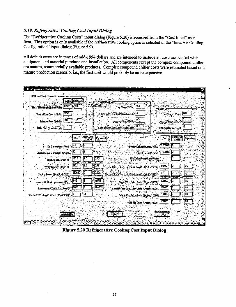
5.19. Refrigerative Cooling Cost Input Dialog

The “Refiigerative Cooling Costs” input dialog (Figure 5.20) is accessed from the “Cost Input” menuitem. This option is only available if the refrigerative cooling option is selected in the “Inlet Air CoolingConfiguration” input dialog (Figure 5.9).

All default costs are in terms of mid-1994 dollars and are intended to include all costs associated withequipment and material purchase and installation. All components except the complex compound chillerare mature, commercially available products. Complex compound chiller costs were estimated based on amature production scenario, i.e., the fwst unit would probably be more expensive.

, ..... . , .. . . .. .:,.- - .::.2:. . --:$ 7,-.,..,, . . . . . .. . ., .,-., . ;,. .- ,-,. ~\ .;,--, ”..--–:,2:- ‘ :-; - ~’. ”...:-.--—.-..--- .,-......-.=...:

,:..:

,. ,-~

t .,-~

i —---

, -.. “.”

‘1:;:,.

Figure 5.20 Refrigerative Cooling Cost Input Dialog

27

. .-—..—-. .——.

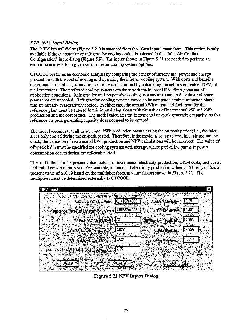
5.20. NPVInput Dialog

The ‘WPV Inputs” dialog (Figure 5.21) is accessed from the “Cost Input” menu item. This option is onlyavailable if the evaporative or refrigerative cooling option is selected in the “Inlet Air CoolingConfiguration” input dialog (Figure 5.9). The inputs shown in Figure 5.21 are needed to petiorm aneconomic analysis for a given set of inlet air cooling system options.

CTCOOL performs an economic analysis by comparing the benefit of incremental power and energyproduction with the cost of owning and operating the inlet air cooling system. With costs and benefitsdenominated in dollars, economic feasibility is determined by calculating the net present value (NW) ofthe investment. The preferred cooling systems are those with the highest NPVS for a given set ofapplication conditions. Refrigerative and evaporative cooling systems are compared against referenceplants that are uncooled. Refrigerative cooling systems may also be compared against reference plantsthat are already evaporatively cooled. In either case, the annual kwh output and fhel input for thereference plant must be entered in this input dialog along with the values of incremental kW and kwhproduction and the cost of fhel. The model calculates the incremental on-peak generating capacity, so thereference on-peak generating capacity does not need to be entered.

The model assumes that all incremental kwh production occurs during the on-peak period; i.e., the inletair is only cooled during the on-peak period. Therefore, if the model is setup to cool inlet air around thecloclq the valuation of incremental kwh production and NPV calculations till be incorrect. The value of

off-peak kWh must be specified for cooling systems with storage, where part of the parasitic powerconsumption occurs during the off-peak period.

The multipliers are the present value factors for incremental electricity production, O&M costs, fuel costs,and initial construction costs. For example, incremental electricity production valued at $1 per year has apresent value of $10.39 based on the multiplier (present value factor) shown in Figure 5.21. Themultipliers m~’ be determined externally to CTCOOL.

Figure 5.21 NPV Inputs Dialog

28

5.21. Input Sunmuuy Dialog

The “Inputs” dialog (Figure 5.22) is accessed from the “View” menu. This dialog prepares a summary ofthe file inputs. The tabulated inputs may also be printed to a file by clicking on the “Output to File”button.

1 Plant T= Sinple Cycle In~:&l Framet 1S0 Heat Rate (BtWkWh)~:~; 1S0 power (MU) 100

1S0 ks=s Flow Rate (lbs@ 2342350Performance Curves Heat Rate

Altitude Adjustment - Slope 0.00000+000!,.. Altitude Adjustment - Intercept I.000ooe+ooo!: First Range Temperature Adjustment - Slope 9.5ooooe-ool

First Range Temperature Adjustment - Intercept 8.33300 e-004!,

‘1Tenperatuze Helm Uhich the First Range Applies 60

~.:,,Second Range Temperature Adjustment - Slope 1.000ooa+ooo

Second Range Temperature Adjuetnent - Intercept 1.66600-003,.. Temperature Belov Vhich the Second Range Applies 150.

Third Range Temperature Adjustmnt - Slope 1.000ooe+oooThird Range Temperature Adjustment Intercept 0.00000-000

nperature Belov Which the Third Range Applies>150. OSxhaust pressme Drop Adjustmnt - Intercept 1.66600-003.“,. u!>..4a:+. &&.L*.L-xu..nn 4 nnnnntian.n

I ““ :’ . ; > ‘:-;<: “.::;::;<:;:! .+--.~. “’-:””. .,.2- ,- - .%

./-., .

! - . .;” ,:,”. ---- -, - . - - .. , .& ..:,. :., ,: .-.1 -. -:”.....”.”: ~ >T.’-?!z: =.--Y-... - . .

Figure 5.22 Echo of Inputs Dialog

5.22. Gas TurbinePerformanceAnalysis OutputDialog

The “GT Analysis Results” dialog (Figure 5.23) is accessed from the “Analysis” menu. After all theinputs are selected/entered, the annual perilormance of the gas turbine maybe simulated. FirsL theweather data must be read by clicking the button “Get Weather Data” in Figure 5.23. After the weatherdata are processed, the button “Run GT Analysis” maybe clicked to simulate the gas turbineperformance. This button will be disabled until the weather data file is processed. Afler the analysis iscompleted, the results are tabulated in the output bo~ as shown in Figure 5.23. The tabulated results mayalso be printed to a file by clicking on the “Output to File” button.

29

—. .——. —— .-.

with the Ueather File

Number of Operating HoursNumber of Active Cooling Hours

Annual Energy Output (IfUh)Average Power (lilJ)

Annual-Fuel (dtujAverage Heat Rate (kHtu/kt?h)

Reference Power (kWh) at Max. EnthalpyHzs=e Povsr (kWh) at Mas. Enthalpy

Peak Power Conditions and ValueMinimum Power Conditions and Value

Peak Heat Rate Conditions and ValueMinimum Heat Rate Conditions and Value

Peak Air Flow Rate Conditions and Valuellinimim Air Flow Rate Conditions and Value

,IR COOLING LOAD OUTPOTPeak Hourly 1st Stage Cooling bad (mmHtu/h)

Annual 1st Stage Cooling Load (mmHtuh)Average Hourly 1st Stage tiling Ioad (mmHtu/h)

PEAK ENERGY NON-STORAGE CASE (adjusted for Genrator CooPeak Hourly 1st Stage Chiller Power (mnBtu/h)

Peak Hotuly 1st Stage Chiller Power (kUh/h)Annual 1st Stage Chiller Energy Consumption (nunHtu)

Annual 1st Stage Chiller Energy Consumption (kWh):or Results with the %athsr File

li

524.000524.00053807.742102.687625350.12511.6227 22 16 2034 1 15 914 1 16 914 1 15 914 1 16 914 1 15 914 1 16 914 1 15 91

If...:1

1/-~.,,7,. ,,.

.,x

1ii”:,,~:87.598 27102.686

,:.:‘,:

102.686102.686 /$+11621.979 :;;11621.979

I2374070.250 ,?:;2374070.250 f “:.:

7 22 16 203 S2487780.19170813952.00036585524.000

.ng Factor)7 22 16 203 85.3147 22 16 203 24996.785

30683.9148990306.000

Figure 5.23 Gas Turbine. Performance Analysis Output Dialog

5.23. CoolingEquipment SizingOu@utDialog

The ’’Cooling Equipment Sizing’’results dialog (Figure 5.24)may beaccessedfrom the ’’Analysis’’menuonly after thegasturbine annual pefiomace isstiulated. Thetabulated results mayalso beptinted toafilebyclickingon the ’’OutputtoFile” button.

5.24. CoolingEquipment CostsOu@utDialog

The ’’CoolingEquipment Costs’’ outputdialog (Figure 5.25)may beaccessedfrom the ’’Analysis’’menuonlytier stiulatig tiegm~bhe aualpefiomace adsizing tiecooling equipment. Thetabulatedresults may also be printed to a file by clicking on the “Output to File” button.

30

I :Ii,:.~~:

I!.I_:.1.

‘1.

:1?,,.

Non-Storage 1st Stage Chiller Size (mmBtu)Cooling Coil UA (Btu/F-h) 7221’203 ‘51121’8”00[:2869150.250

Generator Cooling Heat Eschanger Area (sf) 333.255Chilled water circulation loop size [42/52 F]. (gpn) 8740.971

Chilled vater generator loop size [42/52 F] (gpa) 437.048Psek PllllpPover (kV) 262.229

I

p

Annual Pumping Energy @nsumptiou (kWh) 95777.453Generator Ccaling Loop Peek Punp Ppver (kV) 13.111

,:

Generator Cooling Loop Annual Pumping Energy (kWh) 4788.868,:;:<

Lst Stage tiling TowerI.<;1,:;!

Peak Heat Rejection (Btu/h) 134106272.000~&

Uater Pipe Sizing (gpm) 26799.814Peak Water Pumping Pover (kW) 535.996

1:

!..,

Annual Water Pumping Energy (kWh) 195769.078,-..

Chill= Paresitic Power (kW) 62.460,..

Annual Chiller Parasitic Enargy (kWh) 22813.268

1’

I:..,<..Peak Fen Power (kW) 167.633

Annual Fan Energy (kWh) 61226.785,.7.,?...:

‘Aunual WaterLst Stage HRSG Sizing

Consumption (gals) 6094697.500 i?.,.-:

Figure5.24Cooling Equipment Sizing Calculations

... .. .-,- ~, : .:-- : .-. .“4:.. .,.-—--?m+~.?,. y+-.: ,..~..r<....-..-.-<.-.~~e.;.;”..-: .:-~ *-. =..-:-=. --: -:-. .; --. .-:,. --~ =. T.+:. -e:: -r>:.:,:,+7-..,..‘.‘-...+: -%$++<%,~Td*=.b-.:,: i ,-.7:+-, . . ..+,’

- ‘~-:.:-< . ‘:.-~:G..:: .-$- -. . .-J.......+-- ....:..-.. . .,~-----...__ ...... ---- .............. :-.:...%. ...4 .... . ..

.- ,. :,.-.. ,. :.

. . .. :.:.:.

~ tit Information

-% ....,,~....?

@e: Double .Stage Lithium Sromide - 1st Stage Chiller

cost ($/ton): 650.000O&M cost (as Z of initial cost): 5.000

cost ($): 3203049.750O&l!ICosts ($): 160152.484

Lst Stage air cooling coil

-t ($/[Btfi-f]):O&if-t (as X of initial zest):

Cnst ($):O&H -ts ($):

1st Stage generator ccoling rnil

G5t (s/ft”2)”o. sll:0&H cOst (as Z of initial -t):

Cc=st (s):C&M costs (s):

1st Ammnnia circulation zest

Czst (1W15.000)A0.6:O&M cost (as Z of initial cost):

Gist ($):w Zests ($):

&t (S) [generator lwp]:O&H costs ($) [generator loop]:

1st Steam/Condensate cost

0.2002.000S73830.06311476.601

865.0001.00016832.756168.328

54000.0003.0000.0000.0000.0000.000

Figure 5.25 Cooling Equipment Cost Estimates

31

——

5.25. A?PVCalculations Results Dialog

The ‘TJPV Calculations” results dialog (Figure 5.26) maybe accessed from the “Analysis” menu onlyafter simulating the gas turbine annual performance, sizing the cooling equipment and estimating thecooling equipment costs. The tabulated results may also be printed to a file by clicking on the “Output toFile” button.

.

.— .. . . .. —. . .- —-.—.-—..~ . ,.:= .-:~~-&=-;:5yw..T..:7:7-ZW.ay-...-,-r-------.:.y-:;,.-.~-. --.-..-, m -1 — ., 0

/ir. : ----- --- .,,:,,.:,.. <.. ~., -...... ? .. ,>. ::...: C+.*, -,. . . . ,.:.-.,+; :.::: -.,- ,+: ..:, +*--.,.,. -..,-.

- ---3 .-,-. . .-,, . . . 2 .-..,.->.7-- . .-. E ~:r...

. $ .. . . . - .,:, --. .~-:.>.+,>-.,., ,.& .. - ~e_ ,.,.;..+.:.,- - ,Wy..*

~ .J’ Output frum NPV ruutine...

il~j~

~,>j~Net on-peak power generated (kW) 18463.039 [“;”’

i .“~:+,. : Net fuel (S) 55981.500

}:&<.l-.&~& NW (s) 8423581.000

1~’.

(lfwh) 7322550.500!,. .,\ y;.

1

!>!,,-,:., ... ‘.

(kwh) 1600610.875 +?:~::

~.‘j.

1

. -,{ :,].~.:,.4;:

\,..,: p,::‘

1’”:Ii;.

Incremental power cost ($/kw);.<..:: 182.579

$:;+.-\:..:,.-....

1:.;:

?., .,:,On-Peak kW portion of NPV ($)

I

;;“.-.12086514.000

,<-..!;<;:

~+<j:i %

~:,::

/:.:_.-’On-Peak Wb portion of NPV ($) 2891367.500.:.-..

\i:,::

i.,.; Il.,-

Figure 5.26 NPV Calculations Results

32

6. Sample Case

A sample case, including both the inputs and outputs from the CTCOOL software, is presented in thissection.

The various inputs are shown in Figures 6.1 through 6.12. The gas turbine is assumed to operate onweekdays between 2 p.m. and 6 p.m. (4 hours) for the months of April through September. The inlet aircooling schedule is identical to that of the gas tirbine operating schedule.

Fignre 6.1 Project Information

33

.— .——

Figure 6.2 ISO ~ting for the Industrial Frame Gas”Turbine

Figure 6.3 Heat Rate Performance Coefficients

34

Figure 6.4 Power Performance Coefficients

Figure 6.5 Air Flow Rate Performance Coefficients

35

..—— — —.

Figure 6.6 Inlet Air Cooling Configuration

Figure 6.7 Refrigerative Cooling Configuration

36

Figure 6.8 Vapor Compression Performance D’ata

Figure 6.9 Refrigerative Cooling Sizing Inputs

37

—. ..——— ————.. —.

:[-& ., i=< !.....-..” --”-.,-.,:.:’+ . *-.’.-=--.SF :- -=- ‘‘.: .’‘-:’. .,-,-,. ..... ... .... .< . -.,... ...>.,....-. ..... -. .-,+-. .+.-- 1 CIa-,ak= - ,. .::..>2.:. ... -_ .-4,%.* . .- ..- G2.”4----- ... .. . .. ..-_..+ .--,,

Fi~re 6.10 Thermal Storage Configuration

38

.. --—” . . —--. — ~ —.. ,-—. . . . . . . . . .

.,.< - ..;.;,:2:-,:.:,:,--7------

.Z.:-.%e-,+H&*-&.G.&@&t .s:,.,..::..-...-@.

] J%&ctwiilEq$/wf$...IY’LJ!!L

.... ,-

......

Figure 6.11 Refrigerative Cooling Costs

39

—- . . . ..

Figure 6.12 NPV Inputs

6.1. AnnuaI, Peak andiklhimum Vaks for Selected Performance Parameters

Annual gas turbine performance, along with the minimum and peak values for various pefiormanceparameters, is listed below. Also shown below are the annual and peak-cooling loads. For the peak andthe minimum values, the first four figures represent the month, day of the month, hour of the day, and dayof the year, respectively, while the last figure represents the actual value of the variable.

GAS TURBINE PERFORMANCE

Number of Operating Hours

Number of Active Cooling HoursAnnual Energy Output (MWh)Average Power (MW)Annual Fuel (mmBtu)Average Heat Rate (kBtu/kWh)Reference Power (MW) at Max. EnthalpyBase Power (MW) at Max. EnthalpyPeak Power Conditions and Value (MW)Minimum Power Conditions and Value (MW)Peak Heat Rate Conditions and Value (kBtu/kWh)Minimum Heat Rate Conditions and Value (kBtu/kWh)Peak Air Flow Rate Conditions and Value (lb/h)Minimum Air Flow Rate Conditions and Value (lb/h)

52452454777.2104.537631800.511.5348 20 15 232 85.74 1 15 91 104.54 8 18 98 105.34 1 15 91 104.54 1 16 91 11.5344 8 18 98 11.5154818 98 23912074 1 15 91 2381240

AIR COOLING LOAD OUTPUTPeak Hourly 1st Stage Cooling Load (mmBtu/h) 8 20 15 232 62.650Annual 1st Stage Cooling Load (mmBtu) 20155.80Average Hourly 1st Stage Cooling Load (mmBtu/h) 38.465Peak Daily “lst Stage Cooling Load (mmBtu/day) 231.407

40

+,-r. ,

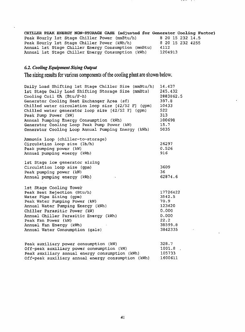
CHILLER PEAK ENERGYNON-STORAGECASE (adjusted for Generator Cooling Factor)Peak Hourly 1st Stage Chiller Power (mmBtu/h) 8 20 15 232 14.5Peak Hourly 1st Stage Chiller Power (kWh/h) 8 20 15 232 4255Annual 1st Stage Chiller Energy Consumption (nunBtu) 4112Annual 1st Stage Chiller Energy Consumption (kWh) 1204913

6.2. Cooling Equipment Sizing Output

Thesizingresultsforvariouscomponentsofthecoolingplantareshownbelow.

Daily Load Shifting 1st Stage Chiller Size (mmBtu/h)1st Stage Daily Load Shifting Storage Size (mmBtu)Cooling Coil UA (Btu/F-h)Generator Cooling Heat Exchanger Area (sf)Chilled water circulation loop size [42/52 F] (gpm)Chilled water generator loop size [42/52 F] (gpm)Peak Pump Power (kW)Annual Pumping Energy Consumption (kWh)Generator Cooling Loop Peak Pump Power (kW)Generator Cooling Loop Annual Pumping Energy (kWh)

Ammonia loop (chiller-to-storage)Circulation loop size (lb/h)Peak pumping power (kW)Annual pumping energy (kWh)

1st Stage ice generator sizingCirculation loop size (gPm)Peak pumping power (kW)Annual pumping energy (kWh)

1st Stage Cooling TowerPeak Heat Rejection (Btu/h)Water Pipe Sizing (gpm)Peak Water Pumping Power (kW)Annual Water Pumping Energy (kWh)Chiller Parasitic Power (kW)Annual Chiller Parasitic Energy (kWh)Peak Fan Power (kW)Annual Fan Energy (kWh)Annual Water Consumption (gals)

Peak auxiliary power consumption (kW)Off-peak auxiliary power consumption (kW)Peak auxiliary annual energy consumption (kWh)Off-peak auxiliary annual energy consumption (kWh)

14.437245.4322883862.5397.81043352231310069815.75035

262970.526916

36093662874.6

177264223542.570.91234200.0000.00022.238599.83842335

328.71001.81057331600611

41

—.-—— --.--—. ———

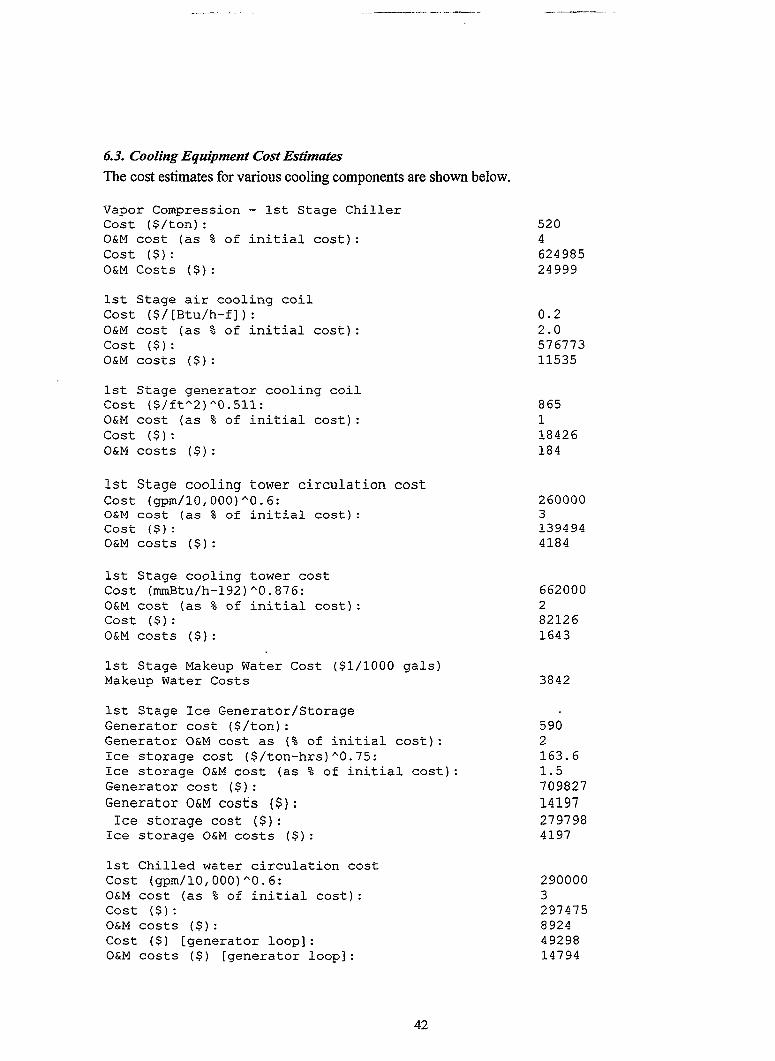
6.3. Cooling Equipment Cost Estimates

The cost estimates for various cooling components are shown below.

Vapor Compression - 1st Stage ChillerCost ($/ton):O&M cost (as % of initial cost) :cost ($):O&M Costs ($):

1st Stage air cooling coil

Cost ($/[Btu/h-f]):O&M cost (as % of initial cost):cost ($):O&M costs ($):

1st Stage generator cooling coil

cost ($/ft’’2)’’511:l:O&M cost (as % of initial cost):cost ($]:O&M costs ($):

1st Stage cooling tower circulation costCost (gpm/10,000)A0.6:O&M cost (as % of initial cost) :cost ($):O&M costs ($):

Ist Stage cooling tower cost

Cost (mmBtu/h-192)A0.876:O&M cost (as % of initial cost):cost ($):O&M costs (.$):

1st Stage Makeup Water Cost ($1/1000 gals)Makeup Water Costs

1st Stage Ice Generator/StorageGenerator cost ($/ton):Generator O&M cost as (% of initial cost):Ice storage cost ($/ton-hrs)A0.75:Ice storage O&M cost (as % of initial cost):Generator cost ($):Generator O&M costs ($):

Ice storage cost ($):Ice storage O&M costs ($):

1st Chilled water circulation costCost (gpm/10,000)’’O.6:O&M cost (as % of initial cost):cost ($):O&M costs ($):Cost ($) [generator loop]:O&M costs ($) [generator loop]:

520462498524999

0.22.057677311535

865118426184

26000031394944184

6620002821261643

3842

5902163.61.5709827

141972797984197

290000329747589244929814794

42

1st stage storage water charging cost (ice loop)

Cost (gpm/10,000)A0.6:O&Mcost (as % of initial cost):cost ($):O&Mcosts ($):

1st Ammonia circulation cost (chiller-to-storage)Cost (lb/h/15,000)A0.6:O&M cost (as % of initial cost):cost ($):O&M costs ($):

System control costFixed Cost ($):O&M cost (as % of initial cost):O&M costs ($):

Plant electric cost

Fixed Cost ($):O&M cost (as % of initial cost):O&M costs ($):

Peak transformer costCost ($ kW)A0.4359:O&M cost (as % of initial cost):cost ($):O&M costs ($):

Total capital cost ($)Total O&M cost ($)

6.4.Net Present Value Outputs

Thenetpresentvalue (NPV)outputsare shownbelow.

Net

Net

Net

Net

NPV

on-peak power generated (kW)on-peak energy generated (kWh)off-peak energy consumed (kWh)

fuel ($)

($)

Incremental power cost ($/kW)On-Peak kW portion of NPVOn-Peak kWh portion of NPV

Off-peak kWh portion of NPV ($)O&Mportion of NPV ($)Fuel portion of NPV ($)

Capital portion of NPV ($)

1000003542571628

540003756282269

250000615000

10000022000

555321128682257

337095598339

184637322551

1600611

559828423581

182.6120865142891368

-324323-1021845-1804480

-3403653

I

43

.. . ... . .. .——

7. Reference

Brown, D.R., S. Katiparnul% and J.H. Konynenbelt. 1996. A Comparative Assessment of AlternativeCombustion Turbine Inlet Air Cooling Systems. PNNL-1 0966. Pacific Northwest National Laboratory,Richkmd, Washington.

45

Appendix A

Model Structure

Appendix A Model Structure

The two flow-charts show the logical flow of the model structure.

+ ,

Cures for HeatRate, Power, Air

flow Rate

&“$+%iE=l

+

lEnterGasTwbirk21 A

e“”+kEnter Refrigerative

v

Enter Cost forRefrigerative Cooling

Components and NW

\Inputs

Figure A.1 Schematic of the CTCOOL Model Structure

A.1

aCalculate adjustedPower, Heat Rate,

Air Flow Rate

Update Mininum

7&

and Peak ValuesCalculate Average Daily/ for Selected

Weekly Outdoor outputsConditions for Siiing

Thermal StorageComponents

YesThermalStorage

.OJ

BWeatherFile

T

L-JOutput Annual

Performance of GasTurbine and Minimumand Peak Values for

Selected Outputs

RefrigerativeCooling

+@

Update AnnualPerformance for

Refrigeratiie Selected Outputs

Cooling

)

I*

Size Cooling/Storage

Equipment

Calculate NetPresent Values

Estimate the Costof CoolingEquipment

Figure A.2 Schematic of the CTCOOL Model Structure (cont.)

A.2

Appendix B

Custom Weather File Format

.

Appendix B Custom Weather File Format

Several weather files are provided with the sotiare; these files have been derived from the TMY weathertapes, However, the user can use a custom weather file for the analysis. The format of the weather file is

shown in Table B 1, with sample data shown in Table B2. The file should be prepared in ASCII “space-delimited” format.

Table B1 - Format for the Custom Weather File

Column Input1 Month2 Day of Month3 Hour of Day4 Day of Year5 Day of Week (l=Sunday, 2=Monday, 3=Tuesday, 4=Wednesday, 5=Thursday,

6=Friday, 7=Saturday)6 Dry-Bulb Temperature (“F)7 Wet-Bulb Temperature (“F)8 Dew-Point Temperature (“F)

Table B2 - Sample Weather Data for Houston

Day of Hour Day Day Dry- Wet- Dew

Month of of of Bulb Bulb Point

Month Day Year Week (“F) (°F) (“F)

1 1 1 1 5 52 51 50.1

1 1 2 1 5 52 51 50.11 1 3 1 5 52 51 50.1

1 1 4 1 5 52 51 50.1

1 1 5 1 5 52 50 48.3

1 1 6 1 5 52 50 48.3

1 1 7 1 5 52 51 50.21 1 8 1 5 53 51 49.51 1 9 1 5 53 51 49.51 1 10 1 5 55 51 47.7

1 1 11 1 5 58 51 45

1 1 12 1 5 60 51 43.3

1 1 13 1 5 61 51 41.91 1 14 1 5 61 50 39.61 1 15 1 5“ 62 50 38.51 1 16 1 5 59 48 36.91 1 17 1 5 57 47 36.41 1 18 1 5 54 45 35.41 1 19 1 5 53 44 33.6

1 1 20 1 5 51 43 33.6

1 1 21 1 5 50 43 34.8

1 1 22 1 5 48 42 34.8

1 1 23 1 5 46 41 35.4

1 1 24 1 5 44 40 35.4

The project information dialog (Figure 5.2) provides the user the ability to select a custom weather file bychecking the “User Defined” button. After the “User Defined” button is checked, the “Get File Name”

B.1

...——.— .-—. ——— -

button becomes active and the user can provide the path and the file name of the custom weather file bydouble clicking on the button. It is the user’s responsibility to make sure the data are consistent and arein the order specified (Table Bl).

B.2

Appendix C

Component Sizing

Appendix C Component Sizing ‘

The equations and assumptions used to size cooling system components are presented in this Appendix.

C.1 C’killer Sizing

For direct air cooling applications (without storage) the chiller is sized to meet the peak air cooling load(pacl) and the cooling load required to cool the generatoc

Ist Stage Chiller Size (Btu/h) = Ist Stage pacl x gcf

where “gcf,” the generator cooling factor, is the amount of additional cooling needed for the generator (avalue of 1.05 is the default assumption). When the air is cooled to O°F,!XVOchillers are sized. The fwstchiller meets the peak cooling load required to cool air from the ambient condition to 42°F (lS stage).The second chiller meets the peak cooling load to cool the air from 42°F to O“F(2ndstage).

2ndStage Chiller Size (Btu/h) = 2ndStage pacl x gcf

When daily storage is used, the total load the chiller is required to provide is the sum of the peak daily aircooling load (pdcl), the daily generator cooling load, and the load required to offset the storage anddefrost (ice storage only) losses. For load-shifting storage, the chiller is sized to generate the total loadwhile operating only during the period when there is no inlet air cooling:

Chiller Size, Daily Load-Shifting (Btu/h) = (pdcl x gcf x seff x defQ/nop

where “seff’ and “deff’ are storage and defrost efficiencies, respectively, and “nop” is the number ofhours the chiller can operate when inlet air is not being cooled. For example, if the inlet air is cooled 4hours per day with an electrically-driven chiller, “nop” is 20 hours. For thermally-activated chillers,

“nop” is the difference between the number of plant operating hours and the number of inlet air coolinghours (because the thermal energy required to run the chiller is extracted from the power plant). For load-leveling storage, the chiller is sized to provide the total daily load while operating 24 hours a day (forelectically-driven chillers) or while the plant is operating (for thermally-activated chillers).

Chiller Size, Daily Load-Leveling (Mu/h) = (pdcl x gcf x seff x defl)/op

where “op” is either 24 or the number of plant operating hours. When weekly storage is used, the totalload the chiller is required to provide is the sum of the peak weekly air cooling load, the weekly generatorcooling load ahd load required to offset the storage and defrost (ice storage only) losses. For load-shit%ng,the chiller is sized to generate the total load while operating only during the period when there isno inlet air cooling. The same equations used to size chillers for daily load-shifting and load-leveling areused for weekly load-shifting and load-leveling. The “nop” for weekly storage is either multiplied by 5 or7, for thermally activated chillers, depending on whether the plant operates on weekends or not. Forelectrically-driven chillers with the plant operating on weekends, the daily “nop” is multiplied by 7; whenthe plant is not operating on weekends, the weekly “nop” is:

weekly nop = (daily nop x 5) + 48

C.1

——. ._ ——.—-.

C.2 Storage Sizing

The storage size for daily load-shifting is:

Daily Storage Size, Load-Shifiing (Btu) = (pdcl x gcf)/seff

The storage size for daily load-leveling is:

Daily Storage Size, Load-Leveling (Btu) = (pdcl x gcflseff - (chiller size x noc x de~

where “not” is the number of inlet cooling hours. The storage size for weekly load-shifting is:

Weekly Storage Size, Load-Shifting (Btu) = (pwcl x gcf)/seff - (chiller size x nop x 4 x dell)

where “pwcl” is the peak weekly cooling load. The storage size for weekly load-leveling is:

Weekly Storage Size, Load-Leveling (Btu) = (pwcl x gc~/seff - (chiller size x (not + 24 x 4) x de~

C.3 Inlet Air Cooling CoilSizing

Both the I’t and 2“dstage inlet air cooling coil UAS are sized as follows:

Coil UA Size (Btu/h-°F) = pacl/ T,Im

where” T1.” is the log mean temperature difference. The heat exchangers required to cool the generatorare sized as follows:

Generator Cooling Coil Size (sf) = pacl x (gcf - 1)/( Timx U)

The values used for” Tl~” and “U” are shown in Table C.1.

Table Cl - Tlsssand U Values Used for $iziig Generator Cooling Coil

Mode T1~ uInlet air cooling to 421? or 52°F 35 225Inlet air cooling to O°F

1~ Stage 10 2252ndStage 60 225

C.4 Chilled Water Circulation System Sizing

The chilled water (CW) circulation loop is sized as follows:

CW Circulation System Size (gPm) = pacl / (500.4 x (To- Ti))

C.2

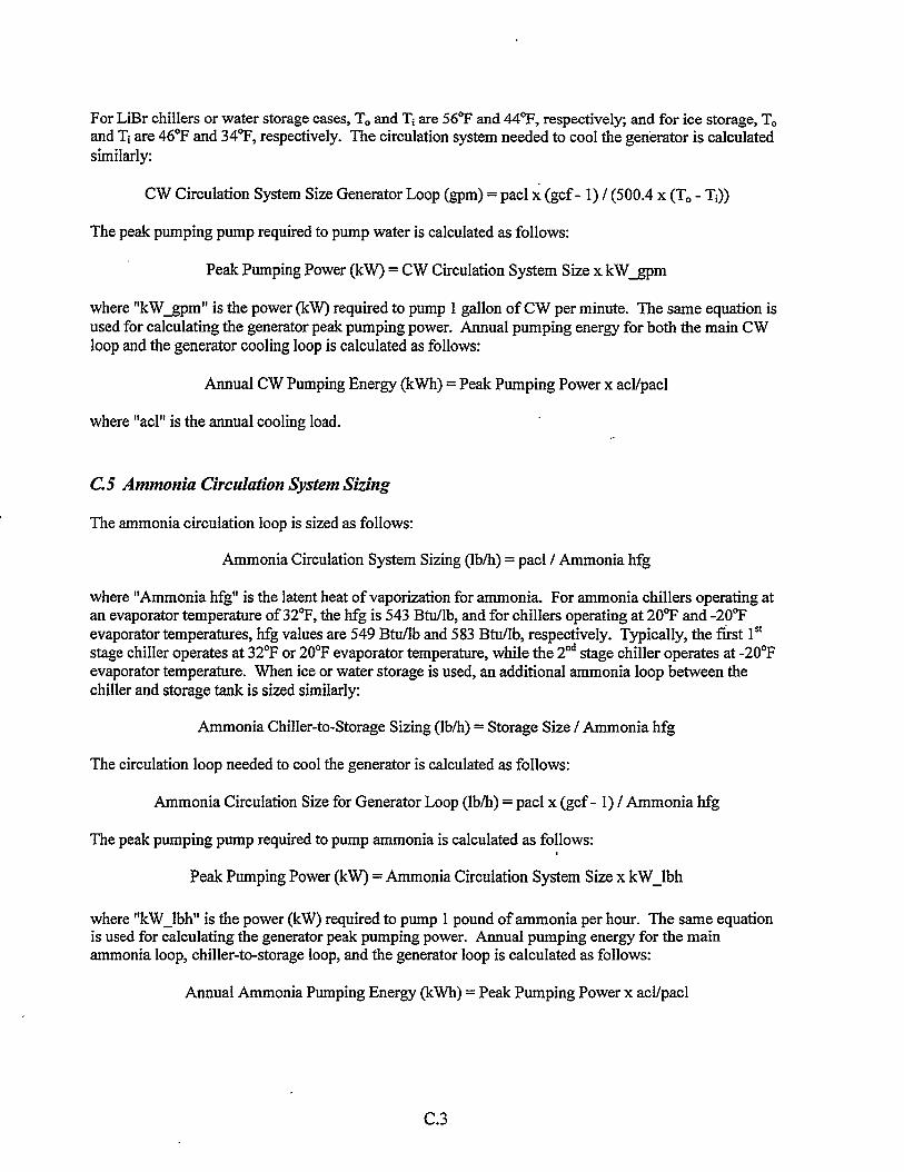
For LiBr chillers or water storage cases, TOand Ti are 56°F and 44”F, respectively and for ice storage, T.and Ti are 46°F and 34”F, respectively. The circulation system needed to cool the generator is calculatedsimilarly:

CW Circulation System Size Generator Loop (gPm) = pacl x (gcf - 1) / (500.4 x (TO- Ti))

The peak pumping pump required to pump water is calculated as follows:

Peak Pumping Power (kW) = CW Circulation System Size x kW~m

where “kW~m” is the power (kW) required to pump 1 gallon of CW per minute. The same equation isused for calculating the generator peak pumping power. Annual pumping energy for both the main CWloop and the generator cooling loop is calculated as follows:

Annual CW Pumping Energy (kWh) = Peak Pumping Power x acl/pacl

where “acl” is the annual cooling load.

C.5 Ammonia Circulation System Sizing

The ammonia circulation loop is sized as follows:

Ammonia Circulation System Sizing (lb/h) = pacl / Ammonia hfg

where “Ammonia hfg” is the latent heat of vaporization for ammonia. For ammonia chillers operating atan evaporator temperature of 32”F, the hfg is 543 Btu/lb, and for chillers operating at 20”F and -20”Fevaporator temperatures, hfg values are 549 Btu/lb and 583 Btu/lb, respectively. Typically, the At 1‘tstage chiller operates at 32°F or 20”F evaporator temperature, while the 2ndstage chiller operates at -20”Fevaporator temperature. When ice or water storage is used, an additional ammonia loop between thechiller and storage tank is sized similarly

Ammonia Chiller-to-Storage Sizing (lb/h) = Storage Size/ Ammonia hfg

The circulation loop needed to cool the generator is calculated as follows:

Ammonia Circulation Size for Generator Loop (lb/h) = pacl x (gcf - 1)/ Ammonia hfg

The peak pumping pump required to pump ammonia is calculated as follows:

Peak Pumping Power (kW) = Ammonia Circulation System Size x kW_lbh

where “kW_lbh” is the power (kW) required to pump 1 pound of ammonia per hour. The same equationis used for calculating the generator peak pumping power. Annual pumping energy for the mainammonia loop, chiller-to-storage loop, and the generator loop is calculated as follows:

Annual Ammonia Pumping Energy (kWh) = Peak Pumping Power x acl/pacl

C.3

C.6 Ice Generator Sizing

The size of the ice generator is same as the chiller. The circulation loop for the ice generator is sized asfollows:

Ice Generator Circulation Loop Sizing (gPm) = Chiller Size x ice_~mpt / 12000

where “ice~mpt” is the circulation loop flow rate in gallons per minute per ton of chilling capacity.The peak pumping power is calculated as follows:

Peak Pumping Power for Ice Generator (kW) = Chiller Size x ikW_ton / 12000

where “ikW_ton” is the kW per ton of chilling capacity. Annual pumping power is calculated as follows:

Annual Pumping Energy (kWh) = Peak Pumping Power x acl x gcf / (seff x Chiller Size)

C. 7 Chilled Water Generator

The size of the chilled water generator is same as the chiller. The circulation loop for the chilled watergenerator is sized as follows:

CW Generator Circulation Loop Sizing (gPm) = Chiller Size / (12000 x h20~mpt)

where“h20=gmpt” isthecirculationloopflowrateingallonsperminutepertonofchillingcapachy.

The peakpumping power iscalculatedasfollows:

Peak Pumping Power for CW Generator (kW) = Chiller Size / (12000 x wkW_ton)

where “wkW ton” is the kW per ton of chiller capacity. Annual pumping power is calculated as follows:—

Annual Pumping Power (kWh) = Peak Pumping Power x acl x gcf / (seff x Chiller Size)

C.8 Cooling Tower Sizing

The peakheat rejection rate at the cooling tower for both 1Sand 2ndstage is calculated as follows:

Peak Heat Rejection Rate (Btu/h) = Chiller Size x Chiller Heat Rejection Rate/ 12000

where the chiller heat rejection rate varies by chiller technology. The water pipe sizing for the coolingtower is:

Cooling Water Sizing (gPm) = Peak Heat Rejection Rate/ (500.4x T.)

where T, is assumed to be 10“F. The pealcpumping power is calculated as follows:

Peak Pumping Power (kW) = Cooling Water Sizing x ckW~m

C.4

where “ckW~m” is 0.02. Annual pumping energy is calculated as follows:

Annual Pumping Energy (kWh) = Peak Pumping Power x acl x gcf / (seff x Chiller Size)

The peak fan power for the cooling tower is calculated as follows:

Peak Fan Power (kVI) = Peak Heat Rejection Rate x kW_rnmBtu/lE6

where “kW_mmBtu” is 1.25. The annual fan energy consumption is calculated as follows:

Annual Fan Energy (kWh) = (Peak Fan Power x acl x gcf)/(seff x Chiller Size)

C.9 Chiller Parasitic Energy

The LiBr chiller has additional parasitic consumption, which is calculated as follows:

Annual Parasitic (kWh) = (Chiller Size/ 12000x kW_ton) x acl x gcf / Chiller Size

where “kW_ton” is 0.0136 kW/ton for a single stage LiBr chiller and 0.028 kW/ton for a double-stageLiBr chiller.

C.1O Heat Recovery Steam Generators (HRSG)

The heat recovery steam generator for thermally-activated chillers with a simple-cycle power plant issized as follows:

HRSG UA (Btu/h-°F) = Peak Chiller Energy Consumption/ Tlm

where” T1~”is the log mean temperature difference:

T1~= ((gt_fex - feed_t) - (gt_ex - feed_t))/(log((gt_fex - feed_t)/(@_ex - feed_t))

where “gt_ex” is the temperature of the exhaust gas leaving the gas twbine (1000 ‘F) ~d “gt_fex” is thetemperature of the exhaust gas leaving the HRSG. The exhaust gas leaving the HRSG is calculated asfollows:

gt_fex (“F)= gt_ex - Peak Chiller Energy Consumptioti(mass x CPGas)

where “mass” is the mass flow rate of the exhaust gas and a value of 0.25 Btu/ “F-lb is assumed for theexhaust gas CP. The required steam flow is calculated x follows:

Steam Flow (lb/h) = Peak Chiller Energy Consumptionl(Stearn hfg)

A maximum pressure drop equivalent to 10 inches of water is assumed to occur in the HRSG, if all theenergy born the exhaust gas is extracted to generate steam (i.e., if~_fex=300”F).. However, only afraction of the exhaust flow energy is required in most cases to meet the peak energy requirements of thethermally-activated chille~

C.5

.-— — ———.– ———-

Fraction of Energy Required= (gt_ex - gt_fex)/(gt_ex - 300)

The required exhaust airflow to meet the peak chiller energy consumption is calculated as follows:

Exhaust Flow Rate (lb/h) = Chiller Energy Consumption/(Cp Gas x (gt_ex - gt_fex))

C.11 Power Reduction Due to Steam Extraction

Power is lost when a thermally-activated chiller is used with a combined-cycle power plant because thesteam extracted from the combined-cycle to run the chiller would otherwise be used to generatedelectricity. The foregone electricity production is calculated as follows:

Power Reduction (kW) = (-0.0079 + 0.0172x log. (Steam Pressure, psia))

The amount of steam that has to be extracted is calculated as follows:

- Steam Flow (lb/h) = Peak Chiller Energy Consumption/(Steam hfg)

C.6

Appendix D

Performance Analysis

Appendix D Performance Analysis

The performance analysis includes calculation of the power output and fhel consumption of thecombustion turbine, with and without inlet air cooling, plus the parasitic power consumption of inlet aircooling system components. The latter includes compressor power for vapor compression chillem, steamand pump power for absorption chillers, pump power for the various fluid circulation systems, and fimpower for the cooling tower.

Annual performance data are calculated by aggregating petiormance calculated for each operating hour ofthe year, based on hourly weather data. Performance assumptions were developed based on acombination of information collected from equipment vendors and published literature. Specificassumptions are presented below for the power plants and cooling system components.

D.1 Power Plants

Three power plant types were evaluated in this study: 1) simple-cycle industrial turbine, 2) simple-cycleaeroderivative turbine, and 3) combined-cycle (based on an industrial-type turbine). Analysis of inlet aircooling systems requires knowledge of the power plant’s (combustion turbine@ steam turbine, forcombined-cycle plants) petiormance (power output heat rate, and mass flow rate) as a function of variousoperating conditions (altitude, dry-bulb temperature, humidity, turbine inlet pressure drop, and turbine

exit pressure drop). The impact of operating conditions on power output and heat rate directly affect inletair cooling economics, of course, while understanding the impact on mass flow rate is crucial to sizingcooling system components.

Power outpu~ heat rate, and inlet air mass flow rate at ISO conditions (59 “F dry-bulb temperature, 60’%0relative humidity, and sea level elevation), and the correction factors for calculating these performancecharacteristics at non-ISO conditions are presented below for each power plant type. Up to fiveadjustment factors (F 1 for altitude, F2 for dry-bulb temperature, F3 for humidity, F4 for excess inletpressure drop, and F5 for excess exhaust pressure drop) are multiplied by the 1S0 performance tocalculate performance at non-ISO conditions.

SimPle-Cvcle lndtistrial Frame Combustion Turbine

ISO Power Output= 100 MWISO Heat Rate= 11,700 Btu/kWh based on HHVISO Inlet Air Mass Flow Rate= 2,342,346 lb/h.

Power Adjustment Factors:

F1 = 1,0-3.1875 E-5* h; h = altitude, feetF2 = 1.23-3.875 E-3 *T, T = inlet air dry-bulb temperature, “FF3=1.OF4 = 1.0-4.333 E-3 * Pi; Pi = excess inlet air pressure loss, inches H20F5 = 1.0-1.634 E-3 * P.; P, = excess exhaust air pressure loss, inches H20.

D.1

- ..—. .—..——

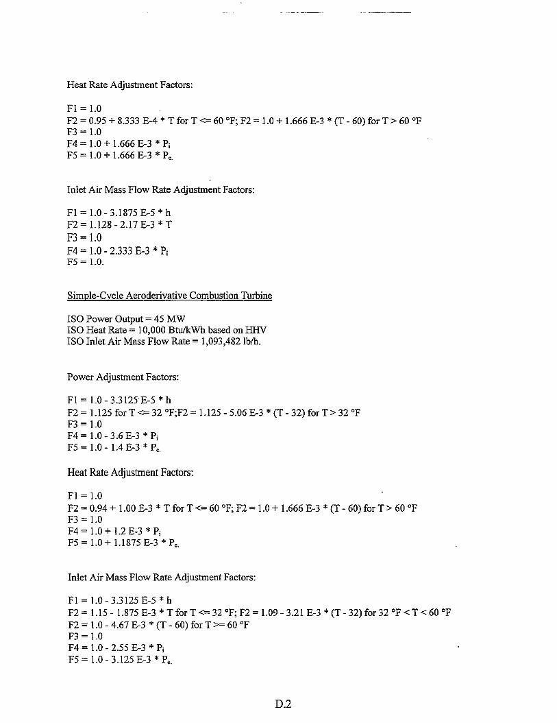
Heat Rate Adjustment Factors:

F1 = 1.0F2 = 0.95 + 8.333 E-4 * T for T <= 60 “F; F2 = 1.0+ 1.666 E-3 *(T - 60) for T >60 ‘FF3=1.OF4= 1.0+ 1.666 E-3 *PiF5 = 1.0 + 1.666 E-3 * P..

Inlet Air Mass Flow Rate Adjustment Factors:

Fl=l.0-3.1875E-5*hF2= 1.128 -2.17 E-3 *TF3=1.OF4 = 1.0-2.333 E-3 *PiF5 = 1.0.

SimPle-CYcle Aeroderivative Combustion Turbine

ISO Power Output= 45 MW1S0 Heat Rate= 10,000 Btu/kWh based on HHV1S0 Inlet Air Mass Flow Rate= 1,093,482 lb/h.

Power Adjustment Factors:

F1 = 1.O-3.3125”E-5 * hF2 = 1.125 for T<=32 ‘F;F2 = 1.125-5.06 E-3 * (T- 32) for T>32 ‘FF3=1.OF4= 1.O-3.6 E-3 *PiF5= 1.0- 1.4 E-3 *P,.

Heat Rate Adjustment Factors:

F1=I.OF2=0.94+ 1.00 E-3 *T for T<=60°F; F2=l.0+ 1.666 E-3 *(T- 60) for T>60°FF3=1.OF4=l.0+1.2E-3 *PiF5= 1.0+ 1.1875 E-3 *P..

Inlet Air Mass Flow Rate Adjustment Factors:

Fl=l.O-3.3125E-5*hF2= 1.15- 1.875 E-3 *T for T<=32°F; F2= 1.09-3.21 E-3 *(T- 32) for32°F<T<600FF2 = 1.0-4.67 E-3 * (T - 60) for T >= 60 “FF3=1.OF4 = 1.0-2.55 E-3 *PiF5 = 1.0-3.125 E-3 * P..

D.2

Combined-Cy61e

ISO Power Output= 225 MWCombustion Turbine Portion = 155 MWSteam Turbine Portion =70 MW1S0 Heat Rate= 7300 Btu/kWh based on HHV1S0 Inlet Air Mass Flow Rate= 3,365,475 lb/h.

Power Adjustment Factors for Combustion Turbine Portion:

Fl=l.0-3.33E-5*hF2=1.22-3.7E-3*TF3=1.OF4= 1.O-3.2 E-3 *PiF5= 1.0- 1.2 E-3 *P..

Power Adjustment Factors for Steam Turbine Portion:

The power adjustment factors for the steam turbine require a more complicated format. In general, steamturbine power is presumed to be proportional to steam production from the HRSG, with an adjustment forthe impact of ambient temperature on condenser temperature. The general form for steam turbine poweradjustment is as follows:

P/PIso = exhaust flow factor* exhaust temperature factor* condenser temperature factor.

Each of these three factors is defined below.

Exhaust Flow Factor = F1*F2*F3*F4*F5, where

F1 = 1.O-3.33ti5 *hF2= 1.12 -2.15 E-3 *TF3=1.OF4= 1.O-2.5G3 *PiF5 = 1.0.

Exhaust Temperature Factor = (Tefiaw- 550)/542, where

TA,W~= 1054+0.517 T+Pi + 0.8 P. for T<=60 “F orT.fi.mt = 1085 + 0.850 (T - 60)+ Pi + 0.8 P. for T >60 “F.

Condenser Temperature Factor =

1 -1.9 E-4* (TW~- 54) for Tti <= 54 “F or1 -9.0 E-4* (TW~- 54) for TWb>54 “F, and

D.3

-. .—

TWb= ambient wet-bulb temperature, “F.

Heat Rate Adjustment Factors for Combustion Turbine Portion:

F1 = 1.0F2=0.94+ 1.00 E-3 *T for T<=60°F; F2=l.0+1.5 E-3 *(T- 60) for T>60°FF3=1.OF4= 1.0+ 1.7 E-3 *PiF5= 1.0+ 1.45 E-3 *P..

Heat Rate Adjustment Factors for Combined-Cycle:

Overall Heat Rate = CT Heat Rate * CT Power/CC Power7300 = CT Heat Rate* 155/225; Reference CT Heat Rate= 10,597 Btu/kWhAdjusted CT Heat Rate = 10,597 * F1 * F2 * F3 * F4 * F5Adjusted CC Power= Adj. CT Power+ Adj. ST PowerAdjusted CC Heat Rate= Adj. CT HR * Adj. CT Power / Adj. CC Power.

Inlet Air Mass Flow Rate Adjustment Factors:

F1 = 1.0-3.33 E-5 hF2=1.12-2.15E-3TF3=1.O

F4 = 1.0- 2.5 E-3 PiF5 = 1.0.

D.2 Chillers

The costand performance of the chiller are key to the cost effectiveness of inlet air cooling systems.Chiller performance is characterized by its coefficient-of-performance (COP), “relative capacity,” heatrejection rate, and, for absorption-type chillers, the steam conditions and additional electric powerconsumption, if any. Performance assumptions for complex-compound, vapor-compression, aqua-ammoni~ and lithium bromide chillers are presented below.

The COP, of course, is the amount of cooling obtained per unit of input energy, with the input and outputmeasured in the same units. The COP varies considerably between chiller types and for the same chillertype, depending on the evaporating and condensing temperature, with the difference between these twotemperatures defined as the “lift.” In general, COP increases as the lift is reduced. Absorption-typechillers also come in single- and double-stage versions. Double-stage chillers use waste heat from thehigher temperature stage to drive the lower temperature stage. A higher COP results, but the double-stageunit is more expensive. COP equations are presented here as a fimction of wet-bulb temperature forexplicit chiller types, number of stages, and evaporator temperatures. The COP equations assume thecondenser temperature is 15 ‘F higher thw the wet-bulb temperature. In general, the wet-bulbtemperature is limited to a minimum of 25 ‘F for COP modeling purposes, with more restrictiveassumptions listed below for lithium bromide chillers.

D.4

Like the COP, the cooling capacity of a chiller is a fimction of the condenser temperature, and isexpressed here as a fimction of the wet-bulb temperature. The chiller cost equations presented in Section8 are based on chiller capacity at “rated” temperature conditions. Capacity is typically less at temperatureconditions corresponding to the peak cooling load. Thus, the “relative” capacity equation must be appliedto adjust the peak chiller capacity to the rated chiller capacity.

All energy absorbed by a chiller at the evaporator and input to the chiller in the form of steam orelectricity must ultimately be rejected at a cooling tower. Thus, heat rejection requirements are directlyrelated to chiller COP and vary considerably, especially when absorption systems are compared to vaporcompression systems.

Comcdex-Comuound Chillers:

CC chiller 1 (CC-l); single stage, 20 ‘F evaporator:

COP= 0.496 -7.0 E-4* Twbrelative capacity = 1.652-0.0079 * Twbsteam temperature =228 “F; pressure = 19 psi% hf~= 960 Btu/lbheat rejection rate = 39,335 Btu/hr per tonparasitic power = O.

CC chiller 2 (CC-2); single stage, 32 “F evaporator:

COP = 0.496-7.0 E-4* Twbrelativecapacity= 1,415-0.0051*Twbsteamtemperature=228 ‘F;pressure= 19psiy hfg= 960Btu/lbheat rejection rate = 39,211 Btu/hr per tonparasitic power = O.

CC chiller 3 (CC-3] double stage, 20 ‘F evaporato~

COP = 0.867-2.5 E-3 * Twbrelative capacity = 1.566-0.0069 * Twbsteam temperature =35 1 ‘F; pressure= 137 psi% hf~= 870 Btilbheat rejection rate = 29,991 Btu/hr per tonparasitic power = O.

CC chiller 4 (CC-4); double stage, 32 ‘F evaporato~

COP = 0.850-1.85 E-3 * Twbrelative capacity = 1.334-0.0041 * Twbsteam temperature =35 1 ‘F; pressure= 137 psiw hf~= 870 Btu/lbheat rejection rate = 29,094 Btu/hr per tonparasitic power = O.

CC chiller 5 (CC-5); single stage, -20 ‘F evaporato~

COP = 0.42-6.75 E-4* Twbrelative capacity = 1.231-0.003 * Twbsteam temperature = 293 ‘F; pressure= 60 psi% hf~=915 Btu/lb

D.5

.. . . . .- .—- ..— —.———-

heat rejection rate = 44,787 Btu/hr per tonparasitic power = O.

CC chiller 6 (CC-6); single-stage, storage lype, -20 ‘F evaporato~

COP= 0.52relative capacity = 1steam temperature = 213 ‘F; pressure= 15 psi% hf~= 969 Btu/lbheat rejection rate = 21,624 Btafhr per tonfor sizing heat rejection equipmentheat rejection rate = 35,076 Btu/hr per tonfor calculating annual heat rejection loadparasitic power = O.

The storage version of the complex-compound chiller is actually an integrated chiller/storagedevice that is sized based on ton-hours rather than tons.

AmmoniaVaporCompressionChillers:

VC chiller 1 (VC-1); 20 “F evaporator:

COP = 14.1277 exp(-O.0144 * Twb)relative capacity = 1.08-0.001 * Twbheat rejection rate = 14,734 Btu/hr per tonparasitic power = O.

VC chiller 2 (VC-2); 32 ‘F evaporato~

COP = 20.1417 exp(-O.0171 * Twb)relative capacity = 1.265-0.0033 * Twbheat rejection rate = 14,334 Btu/hr per tonparasitic power = O.

VC chiller 3 (VC-3); -20 ‘F evaporato~

COP = 5.863 exp(-O.0123 * Twb)relative capacity = 1.008-0.001 * Twb

heat rejection rate = 17,444 Btu/hr per tonparasitic power = O.

Aqua-Ammonia Chillers

AA chiller 1 (AA-l); 20 “F evaporator:

COP = 0.820- 0.00374* Twbrelative capacity = 1.5625-0.0075 * Twbsteam temperature = 252 “F; pressure=31 psi% hf~= 944 Btu/lbheat rejection rate = 34,263 Btu/hr per tonparasitic power = O.

D.6

M chiller 2 (W-2); 32 “F evaporator

COP= 0.857- 0.00372*Twbrelative capacity = 1.5625-0.0075 * Twbsteam temperature =240 “F; pressure =25 psi~ hf~= 952 Btu/lbheat rejection rate = 32,754 Btu/hr per tonparasitic power = O.

AA chiller 3 (AA-3); -20 “F evaporator

COP = 0.8672-0.00635 * Twbrelative capacity = 1.5625-0.0075 * Twbsteam temperature = 315 ‘F; pressure= 83 psizq hf~= 899 Btu/lbheat rejection rate = 42,691 Btu/hr per tonparasitic power = O. .

Lithium Bromide Chillers

LiBr chiller 1 (LiBr-l); single-stage:

COP= 0.671-9.7 E-4* (Twb- 65)’-5relative capacity = 1.22-0.024 * (Twb - 65)steam temperature = 244 “F; pressure= 27 psi% hf~= 950 Btdlbheat rejection rate = 29,200 Btu/hr per tonparasitic power = 0.0136 kW/ton.

The minimum cooling water temperature allowable for single-stage LiBr chillers is 75 ‘F.Therefore, Twb is limited to a minimum of 65 ‘F.

LIBr chiller 2 (LiBr-2); double-stage, 32 “F evaporato~

COP = 1.237-4.258 E-3 * (Twb - 68)1”2relative capacity = 1.074-0.0255 * (Twb - 68)steam temperature = 347 “F; pressure= 130 psiq hf~= 873 Btu/lbheat rejection rate = 21,800 Btu/hr per tonparasitic power = 0.028 kW/ton.

Theminimumcoolingwatertemperatureallowablefordouble-stageLiBrchillersis78”F. Therefore, Twb is limited to a minimum of 68 “F.

D.3 Storage

Storage is a significant component of a CTIAC system, but can be effectively modeled with a few simpleinputs. Thermal losses through the walls of the storage tank are typically no more than 10/0,but other lossmechanisms have a much greater impact. Water storage relies on the creation of a thermocline to separatethe hot and cold portions of the water. The difference between hot and cold temperatures, hence hot andcold bouyancies, is not much in this application of water/thermal storage. Therefore, losses across thethermocline are relatively high. The combined water storage efficiency was assumed to be 85%. Icestorage is really a mixture of water and ice. During discharge, warm return water is sprayed on top of theice to facilitate melting. Here, mixing is not only beneficial, but required. During the charging cycle,however, periodic defrosting of the ice generator is required to release the ice from the evaporator

D.7

.. . . . —.—-

surfaces. The defrost energy increases the refrigeration load and chiller capacity, but unlike the waterstorage losses or the 1°/0loss through the tank walls, it does not affect the capacity of the storage tank.The defrost efficiency factor was presumed to be 85% (i.e., the chiller load and refrigeration capacity areincreased by a factor of 1/0.85 to account for the defrost energy, which must be removed). The defrostefficiency is separate from the ice storage efficiency, which was presumed to be 99°/0.

D.4 Fluid Circulation

CTIAC systems include several fluid circulation loops, with the specific number and type depending onthe type of chiller and storage. Included here are the ammonia loop connecting the chiller evaporator andother chiller components (except for LiBr chillers), the chilled water loop connecting LiBr chillers andstorage with the inlet air cooling coils, the cooling water loop connecting the chiller with the coolingtower, the steam loop connecting the steam source with absorption-type chillers, and storage water loopsconnecting relatively warm storage water with evaporators in the ice generator or water chiller. Thefollowing pumping power rules-of-thumb were established from a collection of published data describingCTIAC systems.

Ammonia Loop Power: 0.005 kW/ton or 2.0 E-5 kW/lb per hr ammonia

Chilled Water Loop Power: 0.03 kW/gpm water

Cooling Water Loop Powe~ 0.02 kW/gpm water

Steam Loop Powe~ 0.03 kW/gpm or 6.0 E-5 kW/lb per hr steam

Storage Charging Water Loop Power

Ice Generation: 0.03 kW/tonChilled Water Generation: 0.02 kW/ton

D.5 Evaporative Cooling

Evaporative cooling towers are used by every chiller to reject heat. In addition, evaporative inlet aircooling is an alternative to refrigerative inlet air cooling. Water consumption for both types ofevaporators is calculated based on the thermodynamic requirement plus a 10% allowance for blowdownand carryover. The inlet air evaporator consumes 0.01 kW/gpm of water circulating through the cooler or0.3 kW/gpm evaporating. The cooling tower fan consumes 1.25 kW/MMBtu per hour of heat rejected.

D.6Auxiliary System Cooling

Cooling the inlet air of the turbine will increase its shaft power output but care must be taken not toexceed the operating capabilities of other power plant components, specifically the generator,transformer, and lube oil system. Depending on the capabilities of these components, supplementalcooling may be required. This study assumed that supplemental cooling equal to 5’%0of the inlet aircooling load would be required. Chillers and storage components were oversized by this factor, and aseparate cooling loop and heat exchanger was provided to cool the auxiliary equipment.

D.8

D. 7 Turbine Inlet and Exit Excess Pressure Drop

Adding an inlet air cooling device increases the compressor pressure drop, resulting in decreased poweroutput and increased heat rate. Although these losses are relatively small compared to the improvementin these same factors achieved from cooling the air, they are significant enough to warrant inclusion in theanalysis. A similar effect occurs if a heat recovery steam generator is added to a simple-cycle turbine toprovide steam for an absorption-type chiller. The increase in exhaust pressure drop also reduces poweroutput and increases heat rate, but by a relatively small amount. The specific assumptions used for excessinlet and exhaust pressure drop are shown below.

Inlet Air Cooling Coil Air-Side Pressure Drop:

Evaporative Cooling: 1.0 in. of waterRefrigerative Cooling to 42 “F: 0.5 in. of waterRefrigerative Cooling to O‘F: 1.3 in. of water

HRSG Air-Side Pressure Drop:

Maximum pressure drop for fill heat recovery = 10 in. waterActual pressure drop =10 in. * (1000 - TJ(1OOO-3OO)T,= calculated stack reject temperature, ‘F

D.8 Combined-Cycle Steam Extraction Power Output Reduction

Absorption-type chillers require a source of low pressure steam. For simple-cycle power plants, anHRSG and related steam/condensate piping are added to provide the steam. In combined-cycle plants,steam is presumed to be extracted from the lower pressure stages of the steam turbine. While noadditional fuel is required in either case (except for the effect of increasing the exhaust pressure when

adding an HRSG), extracting steam from combined-cycle plant’s steam turbine does incur a loss of powerproduction that would otherwise have been produced. The loss increases as the extraction pressureincreases and was described by the following relationship:

kW/lb per hr steam =-0.0079 + 0.0172 In (P)P = steam pressure, psia.

D.9

Appendix E

Cost Analysis

Appendix E Cost Analysis

Initial capital cost and annual operating and maintenance cost estimating equations were developed foreach cooling system component. Cost data acquired from equipment vendors, published literaturedescribing inlet air cooling systems, and cost estimating reference books were the basis for developing theequations. The equations are applied to equipment sizing results to produce system cost estimatespeculiar to each case evaluated.

All costs were estimated in mid-1994 dollars and are intended to include all costs associated withequipment and material purchase and installation. All components except for the complex-compoundchiller are mature, commercially available products. Complex-compound chiller costs were estimatedbased on a mature production scenario, i.e., the first unit would probably be more expensive.

Note that no equations for estimating annual operating labor costs are presented. No incrementaloperating labor is presumed to be required based on advice received from personnel at an operating inletair cooling system.

E.1 Chiller Capital Costs

A strikingobservationforchillersistheextremelyhighcostoftheaqua-ammoniasystemscomparedtothe other options. Otherwise, all chillers increase in cost as the evaporator temperature is lowered, anddouble-stage units cost more than single-stage units. Absorption chiller costs are less sensitive toevaporator temperature than vapor compression chillers, resulting in a significant cost advantage forcomplex-compound chillers at the lower evaporating temperature required for cooling inlet air to O‘F.

LiBrAbsorptionChillers:44 ‘F water, single stage= $480/ton44 ‘F water, double stage= $650/ton.

Complex-Compound Absorption Chillers:-20 ‘F evaporator temperature, single stage= $490/ton+20 ‘F evaporator temperature, single stage= $390/ton+20 ‘F evaporator temperature, double stage= $550/ton+32 “F evaporator temperature, single stage= $380/ton+32 “F evaporator temperature, double stage= $530/ton-20 “F evaporator temperature, single-stage storage= $3 10/ton-hr.

Note: The storage version of the complex-compound absorption chiller integrates thechiller and storage into a single component. The cost for both is based on the required

storage size.

Aqua/Ammonia Absorption Chillers:-20 ‘F evaporator temperature= $3000/ton+20 ‘F evaporator temperature= $2800/ton+32 ‘F evaporator temperature= $2700/ton.

Ammonia Vapor Compression Chillers:-20 ‘F evaporator temperature= $780/ton

E.]

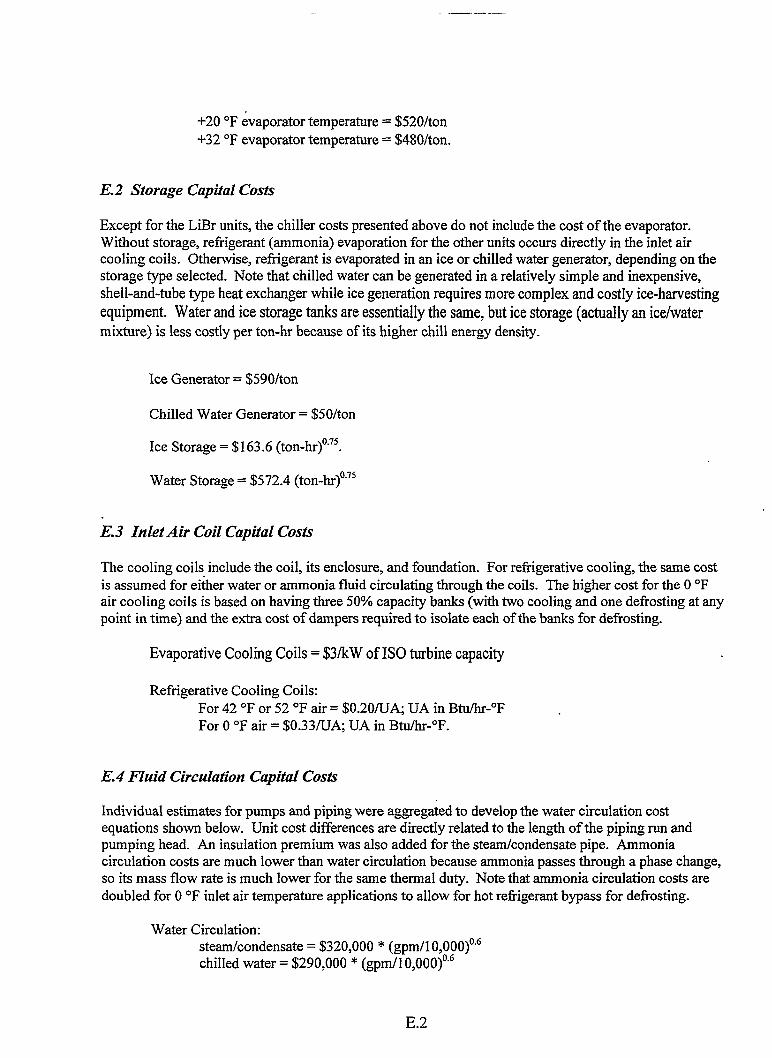
+20 “F evaporator temperature= $520/ton+32 ‘F evaporator temperature= $480/ton.

E.2 Storage Capital Costs

Except for the LiBr units, the chiller costs presented above do not include the cost of the evaporator.Without storage, refrigerant (ammonia) evaporation for the other units occurs directly in the inlet aircooling coils. Otherwise, refrigerant is evaporated in an ice or chilled water generator, depending on thestorage type selected. Note that chilled water can be generated in a relatively simple and inexpensive,shell-and-tube type heat exchanger while ice generation requires more complex and costly ice-hawestingequipment. Water and ice storage tanks are essentially the same, but ice storage (actually an ice/watermixture) is less costly per ton-hr because of its higher chill energy density.

Ice Generator = $590/ton

Chilled Water Generator = $50/ton

Ice Storage = $163.6 (ton-hr)0”75.

Water Storage = $572.4 (ton-hr)0”75

E.3 Inlet Air Coil Capital Cos&

The cooling coils include the coil, its enclosure, and foundation. For refrigerative cooling, the same costis assumed for eiker water or ammonia fluid circulating through the coils. The higher cost for the O“Fair cooling coils is based on having three 50°/0capacity banks (with two cooling and one defrosting at anypoint in time) and the extra cost of dampers required to isolate each of the banks for defrosting.

Evaporative Cooling Coils = $3/kW of 1S0 turbine capacity

Refrigerative Cooling Coils:For 42 “F or 52 “F air = $0.20/UA, UA in Btu/hr-°F .For O‘F air = $0.33KJA; UA in Btu/hr-°F.

E.4 Fluid Circulation Capital Cos&

Individual estimates for pumps and piping were aggrega~ed to develop the water circulation costequations shown below. Unit cost differences are directly related to the length of the piping run andpumping head. An insulation premium was also added for the steam/condensate pipe. Ammoniacirculation costs are much lower than water circulation because ammonia passes through a phase change,so its mass flow rate is much lower for the same thermal duty. Note that ammonia circulation costs aredoubled for O“F inlet air temperature applications to allow for hot refrigerant bypass for defrosting.

Water Circulation:steam/condensate = $320,000 * (gPm/l 0,000)0”6chilled water = $290,000 * (gPm/l 0,000)0.6

E.2

cooling water = $260,000 * (gpmll 0,000)0”6storage charging water = $100,000 * (gpm/10,000)0”6

Ammonia Circulation:For 42 ‘F or 52 ‘F air = $54,000 (lb/hr/15,000)0”GFor O‘F air = $108,000 (lb/hr/15,000)0”G.

ES MiscellaneousEquipment CapitalCosts

Capitalcost estimating equations for other cooling system components are listed below. Heat recoverysteam generators are only used for simple-cycle power plants with absorption-type chillers.

Cooling Tower = $662,000* (MMBtu/hr/192)0”87G

System Controls = $250,000 (fixed for all systems)

Plant Electrical = $100,000 (fixed for all systems)

Transformer = $5,553 * (peak auxiliary kW)O-4359

Heat Recovery Steam Generato~$10,980 * (UA)0”8+$9,658 * (SF)+$918 * (EF)1”2* (1000 - TR)/300

UA = heat transfer surface conductance, Btu/s-°FSF= steam flow, lb/sEF = turbine exhaust flow, lb/sTR = exhaust gas reject temperature after HRSG, “F

Generator Cooling Loop Heat Exchanger = $865 (HTA)O-51*

HTA = heat exchanger heat transfer areq square feet.

E.3

—.—. —-——.

E.6Annual Maintenance Costs

Annual maintenance costs were estimated as a percentage of initial capital cost for each inlet air coolingcomponent. In addition, make-up water, for water consumed at either an evaporative inlet air cooler or acooling tower, was estimated to cost $1/1000 gallons. Maintenance cost estimating percentages are listedbelow.

Component

LiBr chillerNH3/H20 chillerVapor compression chillerComplex compound chillerIce generatorChilled water generatorIce storageWater storageDirect contact evaporative

air coolerInlet air coil

42 ‘F and 52 “F airO“F air

Circulation (pumps and pipes)Cooling towerControlsPlant electicalTransformerHRSGGenerator cooling heat exchanger

Percent.we

5.04.04.03.02.01.01.51.52.0

2.0

3.03.02.06.02.02.03.01.0

E.4

.

No. ofCopies

OFFSITEAinul AbedinD-44 KDA 175350 KarachiPakistan

John S. AndrepontTrigen Energy Corp.79 W. Monroe St. #400Chicago, IL 60603

Chad B. DorganDorgan Associates Inc.7601 Ganser WayMadison, WI 53719-2074

Jerry A. Ebeling7812 Ridgeway Ave.R@OWn, MO 64138-2563

Jon M. Edmonds.Edmonds Engineering Co.PO Box 3591York, PA 17402-2841

Donald EricksonEnergy Concepts Co.627 Rldgely Ave.Annapolis, MD 21401

Alan W. GreenCBI Services Inc.Saint George Dr.Bourbonnais, IL 60914-9584

DavidE.Knebel12830LinkDr.Shakapee, MN 55379

PNNL-12152

Distribution

No. ofCopies

Ted C. KohlenbergerKohlenberger Assoc.611 S. Euclid St.Fullerton, CA 92632-2644

Christopher Michael LandryHenry Vogt Machine Co.Heat Transfer DivisionPO BOX396Denton, TX 76202-0396

Thomas L. Pierson7910 Arbor Hill Ct.Sugar Land, TX 77479

Dharam V. PunwaniAvalon Consulting427 Prairie Knoll Dr.Naperville, IL 60565

Richard J. RademacherVilter Manufacturing Corp.230 Northland Blvd. #334Cincinnati, OH 45246-3650

K.P. RemeshGas Authorily of India Ltd.LPG Recovery PlantG.I.D.C. Industrial EstateVaghodia 391760Dist Barob GujaratIndia

Larry A. Rolison9491 Henderson WayVilla Park, CA 92667-2825

Donald W. Shepherd

Caldwell Energy&Environmental Inc.4000 Tower Rd.Louisville, KY 40219

Distri.1

PNIW-12152

No. ofCopies

OFFSITE continued

Brian Michael SilvettiCalmac Manufacturing Corp.101 W. Sheffield Ave.Englewood, NJ 07631-4804

Anthony Michael SpinelliMunters Corp.Evaporative Cooling108 6* St.Ft. Myers, FL 33907-1554

No. ofCopies

M. Edward Thomas Jr.Alabama Power CompanyPO BOX2641Birmingham, AL 35291-0651

Verle A. WilliamsVA Williams and Associates Inc.5820 Oberlin Dr. #101San Diego, CA 92121-2212

ONSITE

37 Pacific Northwest NationalLaboratory

10 DR Brown, K8-0710 S Katipamul~ K5-1610 S Somasundaram, K5-20

7 Information Release OffIce

Distri.2