Recap for Final - GitHub Pages€¦ · Sreyas Mohan (NYU) Recap for Final 8 May 2019 25 / 33....

Recap for Final

Sreyas Mohan

CDS at NYU

8 May 2019

Sreyas Mohan (NYU) Recap for Final 8 May 2019 1 / 33

Learning Theory Framework

1 Input Space X , output space Y and Action Space A2 Prediction function f : X → A3 Loss Function ` : A× Y → R4 Risk R(f ) = E (`(f (x), y)

5 Bayes prediction function f ∗ = argminf R(f )

6 Bayes Risk R(f ∗)7 Empirical Risk,R̂(f ) - sample approximation for R(f ).

R̂n(f ) = 1n

∑ni=1(f (xi ), yi )

8 Empirical Risk Minimization f̂ = argminf R̂(f )

9 Constrained Empirical Risk Minization


Learning Theory Framework

f ∗ = arg minf

`(f (X ),Y )

fF = arg minf ∈F

`(f (X ),Y ))

f̂n = arg minf ∈F

1

n

n∑i=1

`(f (xi ), yi )

Approximation Error (of F) = R(fF )− R(f ∗)

Estimation error (of f̂n in F) = R(f̂n)− R(fF )


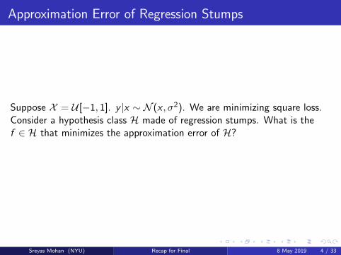
Approximation Error of Regression Stumps

Suppose X = U [−1, 1]. y |x ∼ N (x , σ2). We are minimizing square loss.Consider a hypothesis class H made of regression stumps. What is thef ∈ H that minimizes the approximation error of H?


Solution

Note that f ∗(x) = x and R(f ∗) = σ2.Also R(f ) = E ((f (x)− y)2) = E [(f (x)− E [y |x ])2] + E [(y − E [y |x ])2]We have to minimize E [(f (x)− E [y |x ])2] = E [(f (x)− x)2]The function we are looking for is

f (x) =

{−0.5 −1 ≤ x ≤ 0

+0.5 0 < x ≤ 1


Lasso and Ridge Regression

Linear Regression Closed form Expression (w = XTX )−1XT y

Ridge Regression Solution

Lasso Regression Solution Methods - co-ordinate descent.

Correlated Features for Lasso and Ridge


Optimization Methods

(True/False) Gradient Descent or SGD is only defined for convex lossfunctions.

(True/False) Negative Subgradient direction is a descent direction

(True/False) Negative Stochastic Gradient direction is a descentdirection


Optimization Methods

False

False, but takes you closed to minimizer

False


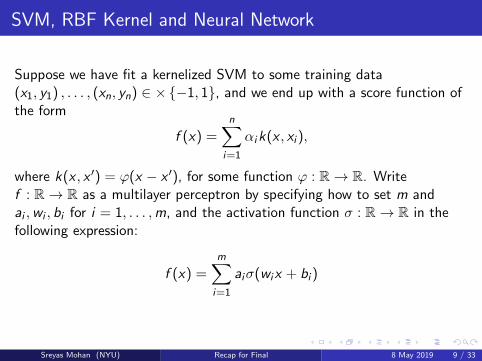
SVM, RBF Kernel and Neural Network

Suppose we have fit a kernelized SVM to some training data(x1, y1) , . . . , (xn, yn) ∈ ×{−1, 1}, and we end up with a score function ofthe form

f (x) =n∑

i=1

αik(x , xi ),

where k(x , x ′) = ϕ(x − x ′), for some function ϕ : R→ R. Writef : R→ R as a multilayer perceptron by specifying how to set m andai ,wi , bi for i = 1, . . . ,m, and the activation function σ : R→ R in thefollowing expression:

f (x) =m∑i=1

aiσ(wix + bi )


Solution

Simply take m = n. Then ai = αi , wi = 1, and bi = −xi . Finally takeσ = ϕ.


Question continued

Suppose you knew which all data points were support vectors. How wouldyou use this information to reduce the size of the network?


Solution

Remove all the nodes corresponding to ai = 0 or non-support vectors.


Maximum Likelihood

Suppose we have samples x1 ≤ x2 ≤ · · · ≤ xn drawn from U [a, b] FindMaximum Likelihood estimate of a and b.


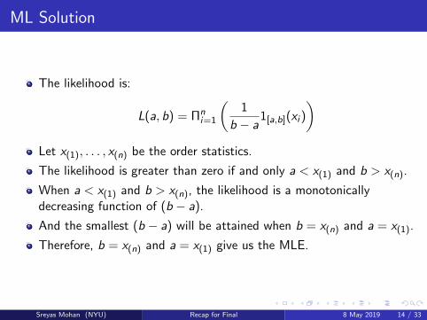
ML Solution

The likelihood is:

L(a, b) = Πni=1

(1

b − a1[a,b](xi )

)Let x(1), . . . , x(n) be the order statistics.

The likelihood is greater than zero if and only a < x(1) and b > x(n).

When a < x(1) and b > x(n), the likelihood is a monotonicallydecreasing function of (b − a).

And the smallest (b − a) will be attained when b = x(n) and a = x(1).

Therefore, b = x(n) and a = x(1) give us the MLE.


Bayesian

Bayesian Bernoulli ModelSuppose we have a coin with unknown probability of heads θ ∈ (0, 1). Weflip the coin n times and get a sequence of coin flips with nh heads and nttails.Recall the following: A Beta(α, β) distribution, for shape parametersα, β > 0, is a distribution supported on the interval (0, 1) with PDF givenby

f (x ;α, β) ∝ xα−1(1− x)β−1.

The mean of a Beta(α, β) distribution is αα+β . The mode is α−1

α+β−2assuming α, β ≥ 1 and α+ β > 2. If α = β = 1, then every value in (0, 1)is a mode.


Question Continued

Which ONE of the following prior distributions on θ corresponds to astrong belief that the coin is approximately fair (i.e. has an equalprobability of heads and tails)?

1 Beta(50, 50)

2 Beta(0.1, 0.1)

3 Beta(1, 100)


Question Continued

1 Give an expression for the likelihood function LD(θ) for this sequenceof flips.

2 Suppose we have a Beta(α, β) prior on θ, for some α, β > 0. Derivethe posterior distribution on θ and, if it is a Beta distribution, give itsparameters.

3 If your posterior distribution on θ is Beta(3, 6), what is your MAPestimate of θ?


LD(θ) = θnh(1− θ)nt

p(θ|D) ∝ p(θ)L(θ)

∝ θα−1(1− θ)β−1θnh(1− θ)nt

∝ θnh+α−1(1− θ)nt+β−1

Thus the posterior distribution is Beta(α + nh, β + nt).

Based on information box above, the mode of the beta distribution isα−1

α+β−2 for α, β > 1. So the MAP estimate is 27 .


Boostrap

What is the probability of not picking one datapoint while creating abootstrap sample?

Suppose the dataset is fairly large. In an expected sense, whatfraction of our bootstrap sample will be unique?


Bootstrap Solutions

1 (1− 1n )n

2 As n→∞, (1− 1n )n → 1

e . So 1− 1e unique samples.


Random Forest and Boosting

Indicate whether each of the statements (about random forests andgradient boosting) is true or false.

1 True or False: If your gradient boosting model is overfitting, takingadditional steps is likely to help.

2 True or False: In gradient boosting, if you reduce your step size, youshould expect to need fewer rounds of boosting (i.e. fewer steps) toachieve the same training set loss.

3 True or False: Fitting a random forest model is extremely easy toparallelize.

4 True or False: Fitting a gradient boosting model is extremely easy toparallelize, for any base regression algorithm.

5 True or False: Suppose we apply gradient boosting with absolute lossto a regression problem. If we use linear ridge regression as our baseregression algorithm, the final prediction function from gradientboosting always will be an affine function of the input.


Solution

False, False, True, False, True


Hypothesis space of GBM and RF

Let HB represent a base hypothesis class of (small) regression trees. LetHR = {g |g =

∑Ti=1

1T fi , fi ∈ HB} represent the hypothesis space of

prediction functions in a random forest with T trees where each tree ispicked from HB . Let HG = {g |g =

∑Ti=1 νi fi , fi ∈ HB , ni ∈ R} represent

the hypothesis space of prediction functions in a gradient boosting with Ttrees.True or False:

1 If fi ∈ HR then αfi ∈ HR for all α ∈ R2 If fi ∈ HG then αfi ∈ HG for all α ∈ R3 If fi ∈ HG then fi ∈ HR

4 If fi ∈ HR then fi ∈ HG


Solutions

True, True, True, True


Neural Networks

1 True or False: Consider a hypothesis space H of prediction functionsf : Rd → R given by a multilayer perceptron (MLP) with 3 hiddenlayers, each consisting of m nodes, for which the activation function isσ(x) = cx , for some fixed c ∈ R. Then this hypothesis space isstrictly larger than the set of all affine functions mapping Rd to R.

2 True or False: Let g : [0, 1]d → R be any continuous function on thecompact set [0, 1]d . Then for any > 0, there exists m ∈ {1, 2, 3, . . .},a = (a1, . . . , am) ∈m,b = (b1, . . . , bm) ∈m, and

W =

- wT1 −

......

...− wT

m −

∈ Rm×d for which the function f : [0, 1]d → R

given by

f (x) =m∑i=1

ai max(0,wTi x + bi )

satisfies |f (x)− g(x)| < ε for all x ∈ [0, 1]d .


Solutions

False, True


Neural Networks

We have a neural network with one input neuron in the first layer, ahidden layer with n neurons and a output layer with 1 neuron. The hiddenlayer has ReLU activation functions. You are allowed to use bias. Explainif the following functions can be represented in this architecture and if yes,give a value for n and set of weights for which this is true.

1 f (x) = |x |


Backprop

Suppose f (x ; θ) and g(x ; θ) are differentiable with respect to θ. For anyexample (x , y), the log-likelihood function is J = L(θ; x , y). Give anexpression for the scalar value ∂J

∂θiin terms of the “local” partial

derivatives at each node. That is, you may assume you know the partialderivative of the output of any node with respect to each of its scalarinputs. For example, you may write your expression in terms of∂J∂α ,

∂J∂β ,

∂α∂sα

, ∂sα∂θ

(1)i

, etc. Note that, as discussed in lecture, θ(1) and θ(2)

represent identical copies of θ, and similarly for x (1) and x (2).

θ ∈ Rm sα = f(x(1), θ(1)) α = ψ(sα) y ∈ (0, 1)

x ∈ Rd sβ = g(x(2), θ(2)) β = ψ(sβ) J = L(α, β; y)

θ(1)

x(2)

θ(2)

x(1)

sα

sβ

α

β

y

J


Backprop solution

∂J

∂θi=∂J

∂α

∂α

∂sα

∂sα

∂θ(1)i

+∂J

∂β

∂β

∂sβ

∂sβ

∂θ(2)i


KMeans


KMeans Solution


Mixture Models

Suppose we have a latent variable z ∈ {1, 2, 3} and an observed variablex ∈ (0,∞) generated as follows:

z ∼ Categorical(π1, π2, π3)

x | z ∼ Gamma(2, βz),

where (β1, β2, β3) ∈ (0,∞)3, and Gamma(2, β) is supported on (0,∞)and has density p(x) = β2xe−βx . Suppose we know thatβ1 = 1, β2 = 2, β3 = 4. Give an explicit expression for p(z = 1|x = 1) interms of the unknown parameters π1, π2, π3.


Recap for Final - GitHub Pages€¦ · Sreyas Mohan (NYU) Recap for Final 8 May 2019 25 / 33....

Documents

Transcript of Recap for Final - GitHub Pages€¦ · Sreyas Mohan (NYU) Recap for Final 8 May 2019 25 / 33....