Reason-Based Rationalization

Franz Dietrich

CNRS & University of East Anglia

Christian List

London School of Economics

This version: 25 November 2013⇤

Abstract

We introduce a “reason-based” way of rationalizing an agent’s choice behaviour,

which explains choices by specifying which properties of the options or choice context

the agent cares about (the “motivationally salient properties”) and how he or she

cares about these properties (the “fundamental preference relation”). Reason-based

rationalizations can explain non-classical choice behaviour, including boundedly ra-

tional and sophisticated rational behaviour, and predict choices in unobserved con-

texts, an issue neglected in standard choice theory. We characterize the behavioural

implications of di↵erent reason-based models and distinguish two kinds of context-

dependent motivation: “context-variant” motivation, where the agent cares about

di↵erent properties in di↵erent contexts, and “context-regarding” motivation, where

the agent cares not only about properties of the options, but also about properties

relating to the context.

1 Introduction

The classical theory of individual choice faces many notorious problems. It is chal-

lenged by empirically well-established violations of rationality due to framing e↵ects,

menu-dependent choice, susceptibility to nudges, the use of heuristics, unawareness, and

other related phenomena. For example, a mere redescription of the same options can

sometimes alter an agent’s choice behaviour. Call this the problem of bounded rational-

ity. The classical theory is also challenged by its inability to explain various intuitively

rational but sophisticated forms of choice, such as choices based on norm-following or

non-consequentialism. It does not distinguish such sophisticated choices from ordinary

⇤This work has been presented on numerous occasions, beginning with the LSE Choice Groupworkshop on “Rationalizability and Choice”, July 2011. We thank the audiences at these occa-sions for helpful comments and suggestions.

1

rationality violations. For example, someone who always chooses the second-largest

(rather than largest) piece of cake o↵ered to him (or her) for politeness violates the

weak axiom of revealed preference and thus counts as “irrational” in the classical sense.

Call this the problem of sophisticated rationality. We suggest that the classical theory’s

di�culty in addressing both problems stems from the lack of a model of how agents

conceptualize options in any given choice context. When we provide such a model, a

unified explanation of many of the challenging phenomena can be given.

Our basic idea is the following. When an agent chooses between several options in

some context, e.g., di↵erent yoghurts in a supermarket, he (or she) conceptualizes each

option not as a primitive object, but as a bundle of properties. Each option can have

a large number of properties; however, the agent considers not all of them, but only a

subset: the motivationally salient properties. In the supermarket, these may include

whether the yoghurt is fruit-flavoured, low-fat, and free from artificial sweeteners, but

exclude whether the yoghurt has an odd (as opposed to even) number of letters on its

label (an irrelevant property), and whether it has been sustainably produced (which

many consumers ignore). The agent then makes his choice on the basis of a fundamental

preference relation over property bundles. He chooses one option over another, e.g., a

low-fat cherry yoghurt over a full-fat, sugar-free vanilla one, if and only if his fundamental

preference relation ranks the set of motivationally salient properties of the first option,

say {low-fat, fruit-flavoured}, above the set of motivationally salient properties of the

second, say {full-flat, vanilla-flavoured, artificially sweetened}.We call an agent’s choice behaviour reason-based rationalizable if it can be explained

in this way. A reason-based rationalization, as we define it, explains an agent’s choice

behaviour by specifying (i) which properties the agent cares about in each choice context

and (ii) how he cares about these properties. We formalize part (i) by a motivational

salience function, which assigns to each context a set of motivationally salient properties,

and part (ii) by the agent’s fundamental preference relation over property bundles.

Crucially, the motivationally salient properties may be of di↵erent kinds. They may

include not only option properties, which options have independently of the choice con-

text (philosophers would call them “intrinsic” properties), but also relational properties,

which options have relative to the context, and context properties, which are proper-

ties of the context alone. “Being fruit-flavoured” and “being low-fat” (in the case of

yoghurts) are option properties; they depend solely on the yoghurt itself. Whether a

yoghurt is the only cherry yoghurt on display or the cheapest one in the supermarket

are relational properties; they depend also on the other available yoghurts. Examples

of context properties, finally, are whether the yoghurts on o↵er include luxury brands

2

(this depends solely on the menu of options) and whether there is cheerful music in the

background (this depends on features of the context over and above the menu).

Reason-based rationalizations can capture two kinds of context-dependence in an

agent’s motivation. First, the context may a↵ect which properties are motivationally

salient, so that the agent cares about di↵erent properties in di↵erent contexts. We

call this context-variant motivation. For example, some contexts make the agent diet-

conscious, others not. Second, the motivationally salient properties may go beyond

option properties and include relational or context properties, so that the agent cares

explicitly about the context or about how the options relate to it. We call this context-

regarding motivation. For example, the agent cares about whether the choice of an option

is polite in the given context or whether there are luxury options available.

Many boundedly rational and sophisticated rational forms of choice can be explained

by these two kinds of context-dependence. Arguably, bounded rationality, such as sus-

ceptibility to framing, nudging, or dynamic inconsistency, often involves context-variant

motivation. Sophisticated rationality, such as norm-following or non-consequentialism,

often involves context-regarding motivation. (Of course, we do not claim that context-

variance is always boundedly rational or that context-regardingness is always sophisti-

cated.)

Note that, while we suggest that agents conceptualize options as bundles of moti-

vationally salient properties, we could not define each option directly as a bundle of

motivationally salient properties. Since an agent may conceptualize the same option in

terms of di↵erent properties in di↵erent contexts, we cannot know the agent’s motiva-

tionally salient properties ex ante; they can be inferred, at most, after observing the

agent’s choices (see Bhattacharyya, Pattanaik, and Xu 2011 for a similar observation).

This paper is structured as follows. In Section 2, we introduce our basic framework

and discuss some examples. In Section 3, we examine the choice-behavioural implications

of the two kinds of context-dependence. In Section 4, we show how choice behaviour can

reveal which properties are motivationally salient and what the fundamental preference

relation is. In Section 5, we explore the prediction of choices in unobserved contexts, a

largely neglected topic in standard choice theory. Importantly, the build-up in the early

sections is needed in order to harvest the fruits of our approach in the later sections.

To the best of our knowledge, our framework is novel. There is, of course, a grow-

ing body of works in decision theory o↵ering non-standard approaches to rationaliza-

tion (e.g., Suzumura and Xu 2001; Kalai, Rubinstein, and Spiegler 2002; Manzini and

Mariotti 2007, 2012; Salant and Rubinstein 2008; Bernheim and Rangel 2009; Man-

dler, Manzini, and Mariotti 2012; Cherepanov, Feddersen, and Sandroni 2013). In the

3

Appendix, we briefly discuss two conceptually related papers by Bossert and Suzumura

(2009) and Bhattacharyya, Pattanaik, and Xu (2011) about the phenomenon of context-

dependence. Our model o↵ers a response to problems identified by them. It also formal-

izes a distinction drawn by Rubinstein (2006) between di↵erent reasons for choice, which

parallels our distinction between context-regarding and context-unregarding motivation.

More extensive reviews of the literature can be found in our earlier papers on preference

formation (Dietrich and List 2012, 2013a,b; Dietrich 2012) and in the monograph by

Bossert and Suzumura (2010).1

2 A general framework

2.1 Observable primitives

Our observable primitives are the following:

• A non-empty set of options, denoted X. Typical elements are x, y, z, ...

• A non-empty set of contexts, denoted K, which can be defined in two ways. On

the classical (“extensional”) definition, each context K 2 K is a non-empty set

K ✓ X of feasible options, which the agent may choose from. On a more general

(“non-extensional”) definition, each context K 2 K induces a non-empty feasible

set [K] ✓ X, but may carry additional information about the choice environment.

Formally, K could be a pair (Y,�) of a feasible set Y (=[K]) and an environmental

parameter �, representing a cue, default criterion, room temperature, background

music, or even the psychological or bodily state of the agent (e.g., sober or drunk).

(This resembles the notion of a frame or “set of ancillary conditions” in Salant

and Rubinstein 2008 or Bernheim and Rangel 2009.) For simplicity, we write K

for [K]. This creates no ambiguity, as it is always clear whether K refers to the

context broadly defined or to the feasible set [K] (e.g., in “x2K”, K refers to [K]).

1In Dietrich and List (2013a,b), we investigated the relationship between motivationally salient prop-

erties (“reasons”) and preferences (related contributions on the logic of preferences include Liu 2010 and

Osherson and Weinstein 2012). The present paper goes significantly beyond those earlier papers, and

there is no overlap in results. In particular, (i) we treat “motivationally salient properties” no longer

as primitives, but as derivable from observable data; (ii) our main observable primitive is now a choice

function, which we seek to explain; (iii) we now introduce relational and context properties, which allow

us us to consider two kinds of context-dependence; and (iv) we develop a framework for predictions

of future choices. For a philosophical discussion of some limitations of classical rational choice theory,

which also supports our current “reason-based” perspective, see Pettit (1991).

4

• A choice function C : K ! 2X , which assigns to each context K 2 K a non-empty

set of chosen options in K (i.e., C(K) ✓ K).

2.2 Properties

When making a choice in context K, an agent e↵ectively selects among di↵erent pairs

of the form (x,K), where x 2 K. We call the elements of X ⇥ K option-context pairs.2

In our framework, the properties of option-context pairs are key determinants of the

agent’s choice. A property is a characteristic that an option-context pair may or may

not have (thus properties are binary). Formally, it is an abstract object, P , that picks

out a subset [P ] ✓ X ⇥K called its extension, which consists of all option-context pairs

that “have” or “satisfy” the property. We assume that the extension of any property is

distinct from ? and X ⇥ K; this rules out properties that are never satisfied or always

satisfied.

Although we often identify a property with its extension, it is sometimes useful to

allow distinct properties to have the same extension, so as to capture those framing

e↵ects in which the description of a property matters. For example, the properties “80%

fat-free” and “20% fat” (in foods) have the same extension but di↵erent descriptions

and may prompt di↵erent choice dispositions in a boundedly rational agent.

We distinguish between three kinds of properties:

Option properties: These are properties whose possession by an option-context pair

depends only on the option, not on the context. Examples are “being fat-free” or “being

a 500g pot” (in the case of yoghurts) and “being an apple” (in the case of fruits).

Formally, P is an option property if

(x,K) 2 [P ] , (x,K 0) 2 [P ] for all x 2 X and K,K

0 2 K.

Context properties: These are properties whose possession by an option-context pair

depends only on the context, not on the option. Examples are “o↵ering more than one

feasible option”, “o↵ering a Rolls Royce among the feasible options”, and – if contexts

are defined as specifying the choice environment over and above the feasible set – the

time, room temperature, or framing of the choice problem. Formally, P is a context

property if

(x,K) 2 [P ] , (x0,K) 2 [P ] for all x, x0 2 X and K 2 K.

2Note that some pairs (x,K) in X ⇥K are “infeasible” in the sense that x /2 K.

5

Relational properties: These are properties whose possesion by an option-context

pair depends on both the option and the context, capturing the relationship between

option and context. Examples are “not being the last available fruit of a particular

kind”, which a polite dinner party guest may care about, or “being the largest item on

the menu”, which a greedy consumer may focus on. Formally, P is a relational property

if it is neither an option property nor a context property.

We call properties that are not option properties context-regarding and properties

that are not context properties option-regarding. Relational properties are context-

regarding and option-regarding.

To explain an agent’s choice behaviour, we consider a set P of potentially relevant

properties, called a property system. This could be specified in di↵erent ways, depending

on the modeller’s goals. It contains the properties that the modeller has at his or her

disposal to rationalize the agent’s choices. The slimmer this set, the fewer patterns of

choice can be explained, i.e., the more demanding our notion of reason-based rationaliz-

ability becomes. We partition P into the set Poption

of option properties, the set Pcontext

of context properties, and the set Prelational

of relational properties. For any option x

and any context K, we write

• P(x,K) for the set {P 2 P : (x,K) 2 [P ]} of all properties of the pair (x,K),

• P(x) = P(x,K) \ Poption

for the set of option properties of x, and

• P(K) = P(x,K) \ Pcontext

for the set of context properties of K.

Each set P(x,K) is assumed to be finite. (Of course, X, K, and P need not be finite.)

A subset of P is called a property bundle.

2.3 An example

We give an example to which we will refer repeatedly. It involves a choice of fruit at

a dinner party (as in Sen’s well-known example of a polite dinner-party guest). Let X

contain di↵erent fruits: apples, bananas, chocolate-covered pears, and possibly others.

Each kind of fruit comes in up to three sizes: big, medium, and small. A choice context

is a non-empty feasible set K ✓ X, consisting of fruits currently in the basket. The set of

possible contexts is K = 2X\{?}. For present purposes, we consider a set of properties

P = {big, medium, small, chocolate-o↵ering, polite}, where

• “big”, “medium”, and “small” are the option properties of being a big, medium,

and small fruit, respectively;

6

• “chocolate-o↵ering” is the context property of o↵ering at least one chocolate-

covered fruit among the feasible options;

• “polite” is the relational property of not being the last available fruit of its kind,

i.e., not being the last apple in the basket, the last banana, the last chocolate-

covered pear, and so on.

We consider four agents whose choice behaviour we will subsequently explain in terms

of the properties in P.

Bon-vivant Bonnie always chooses a largest available fruit. For any K, she chooses

C(K) = {x 2 K : x is largest in K},

where “medium” is larger than “small”, and “big” is larger than both other sizes.

Polite Pauline politely avoids choosing the last available fruit of its kind and only

secondarily cares about a fruit’s size. For any K, she chooses

C(K) = {x 2 K : x is largest in K

⇤ if K⇤ 6= ? and largest in K if K⇤ = ?},

where K

⇤ is the set of all fruits in K that are not the last available ones of their kind.

Chocoholic Coco picks any fruit indi↵erently when no chocolate-covered fruit is avail-

able, but otherwise chooses a largest available fruit, because the smell of chocolate makes

him hungry. For any K, he chooses

C(K) =

(K if no chocolate-covered fruit is available in K,

{x 2 K : x is largest in K} if a chocolate-covered fruit is available in K.

Weak-willed William makes the same polite choices as Pauline when no chocolate-

covered fruit is available, and the same “greedy” choices as Bonnie otherwise, as the

smell of chocolate makes him lose his inhibitions. Formally, C(K) is as in Pauline’s case

when there is no chocolate-covered fruit in K and as in Bonnie’s case when there is.

To explain the behaviour of these agents, we now introduce our central concept.

7

2.4 Reason-based models

A reason-based model of an agent, M, is a pair (M,�) consisting of:

• Amotivational salience function M (formally a function from K into 2P), which as-

signs to each contextK 2 K a setM(K) ofmotivationally salient properties in con-

text K. We require that any contexts with the same context properties induce the

same motivationally salient properties, i.e., if P(K)=P(K 0) then M(K)=M(K 0).

(So, di↵erences in motivation are attributable to di↵erences in context properties.)

• A fundamental preference relation � over property bundles (formally a binary

relation on 2P , on which we initially impose no restrictions). We write > and ⌘for the strict and indi↵erence relations induced by �.

Informally, M specifies which properties the agent cares about in each context, and

� specifies how the agent cares about these properties, by ranking di↵erent property

bundles relative to one another. Note that a reason-based model is always defined

relative to a given property system P.

A reason-based model tells us (i) how the agent conceptualizes options in each con-

text, (ii) how he forms his preferences over the options, and (iii) what choices he is

disposed to make. Formally, according to M:

• Any option x is conceptualized in context K as the set of motivationally salient

properties of (x,K), denoted xK = P(x,K) \M(K).

• The agent’s preference relation in contextK is the binary relation %K onX defined

as follows:

x %K y , xK � yK for all x, y 2 X.

We write �K and ⇠K for the strict and indi↵erence relations induced by %K .

• The agent’s choice dispositions are given by the function C

M : K ! 2X which

assigns to each context the set of most preferred feasible options in that context:

C

M(K) = {x 2 K : x %K y for all y 2 K}.

This defines an improper choice function (“improper” because C

M(K) may be

empty for some K if � is not well-behaved).

We call a choice function C : K ! 2X reason-based rationalizable (relative to P) if there

exists a reason-based model M (relative to P) such that C = C

M. We then call Ma rationalization of C. The four choice functions of our example are all reason-based

rationalizable, as we now show.

8

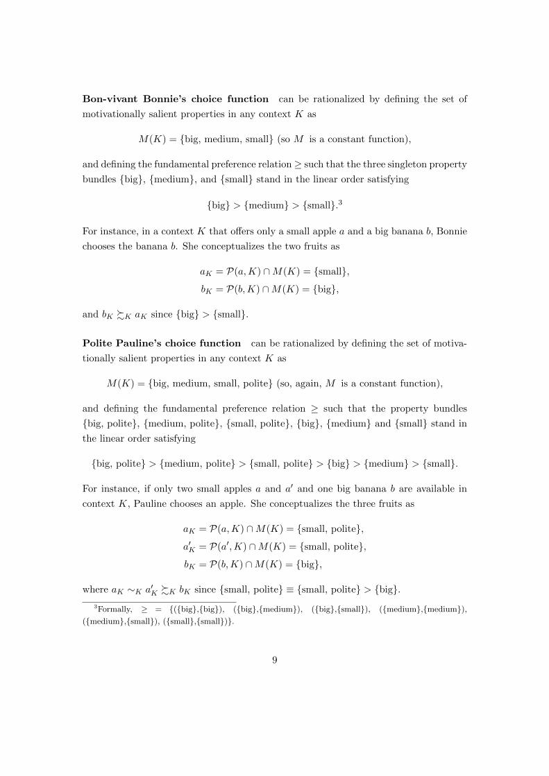
Bon-vivant Bonnie’s choice function can be rationalized by defining the set of

motivationally salient properties in any context K as

M(K) = {big, medium, small} (so M is a constant function),

and defining the fundamental preference relation� such that the three singleton property

bundles {big}, {medium}, and {small} stand in the linear order satisfying

{big} > {medium} > {small}.3

For instance, in a context K that o↵ers only a small apple a and a big banana b, Bonnie

chooses the banana b. She conceptualizes the two fruits as

aK = P(a,K) \M(K) = {small},

bK = P(b,K) \M(K) = {big},

and bK %K aK since {big} > {small}.

Polite Pauline’s choice function can be rationalized by defining the set of motiva-

tionally salient properties in any context K as

M(K) = {big, medium, small, polite} (so, again, M is a constant function),

and defining the fundamental preference relation � such that the property bundles

{big, polite}, {medium, polite}, {small, polite}, {big}, {medium} and {small} stand in

the linear order satisfying

{big, polite} > {medium, polite} > {small, polite} > {big} > {medium} > {small}.

For instance, if only two small apples a and a

0 and one big banana b are available in

context K, Pauline chooses an apple. She conceptualizes the three fruits as

aK = P(a,K) \M(K) = {small, polite},

a

0K = P(a0,K) \M(K) = {small, polite},

bK = P(b,K) \M(K) = {big},

where aK ⇠K a

0K %K bK since {small, polite} ⌘ {small, polite} > {big}.

3Formally, � = {({big},{big}), ({big},{medium}), ({big},{small}), ({medium},{medium}),({medium},{small}), ({small},{small})}.

9

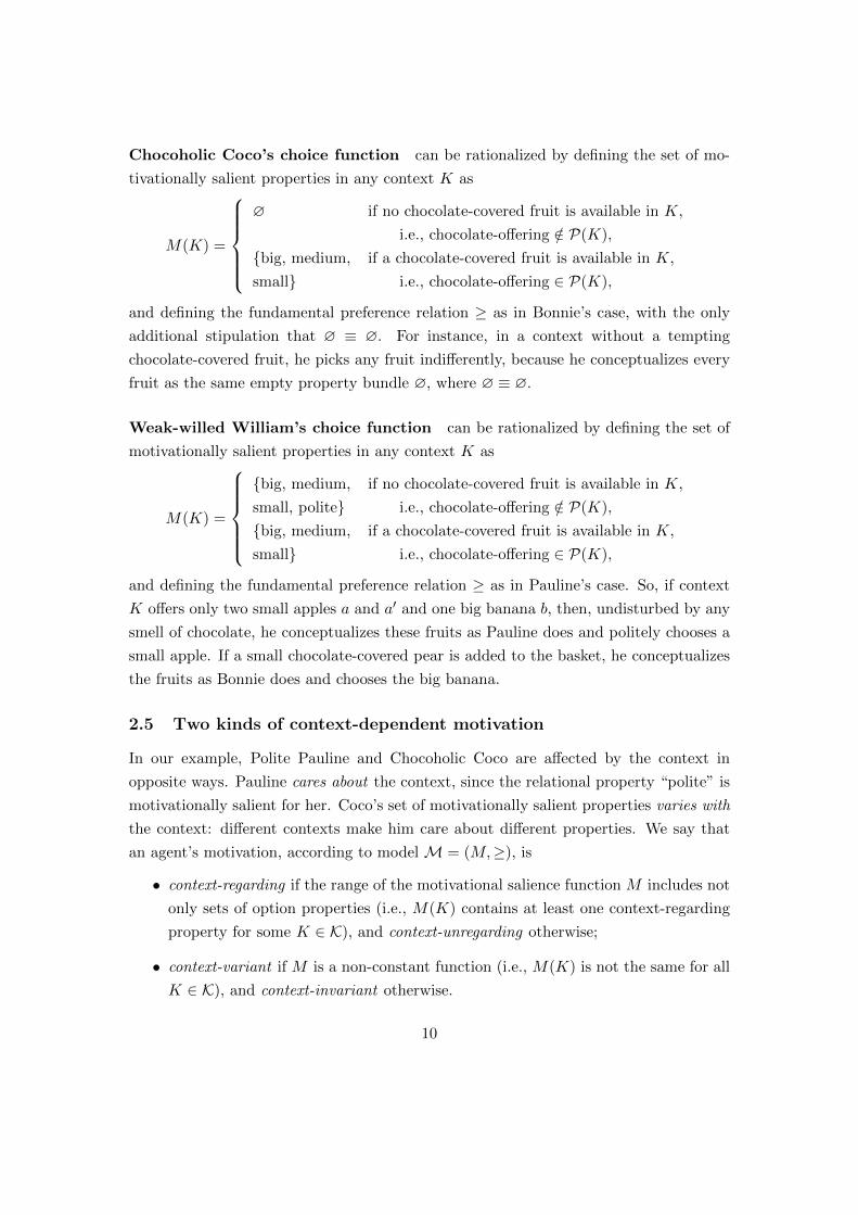
Chocoholic Coco’s choice function can be rationalized by defining the set of mo-

tivationally salient properties in any context K as

M(K) =

8>>>><

>>>>:

? if no chocolate-covered fruit is available in K,

i.e., chocolate-o↵ering /2 P(K),

{big, medium, if a chocolate-covered fruit is available in K,

small} i.e., chocolate-o↵ering 2 P(K),

and defining the fundamental preference relation � as in Bonnie’s case, with the only

additional stipulation that ? ⌘ ?. For instance, in a context without a tempting

chocolate-covered fruit, he picks any fruit indi↵erently, because he conceptualizes every

fruit as the same empty property bundle ?, where ? ⌘ ?.

Weak-willed William’s choice function can be rationalized by defining the set of

motivationally salient properties in any context K as

M(K) =

8>>>><

>>>>:

{big, medium, if no chocolate-covered fruit is available in K,

small, polite} i.e., chocolate-o↵ering /2 P(K),

{big, medium, if a chocolate-covered fruit is available in K,

small} i.e., chocolate-o↵ering 2 P(K),

and defining the fundamental preference relation � as in Pauline’s case. So, if context

K o↵ers only two small apples a and a

0 and one big banana b, then, undisturbed by any

smell of chocolate, he conceptualizes these fruits as Pauline does and politely chooses a

small apple. If a small chocolate-covered pear is added to the basket, he conceptualizes

the fruits as Bonnie does and chooses the big banana.

2.5 Two kinds of context-dependent motivation

In our example, Polite Pauline and Chocoholic Coco are a↵ected by the context in

opposite ways. Pauline cares about the context, since the relational property “polite” is

motivationally salient for her. Coco’s set of motivationally salient properties varies with

the context: di↵erent contexts make him care about di↵erent properties. We say that

an agent’s motivation, according to model M = (M,�), is

• context-regarding if the range of the motivational salience function M includes not

only sets of option properties (i.e., M(K) contains at least one context-regarding

property for some K 2 K), and context-unregarding otherwise;

• context-variant if M is a non-constant function (i.e., M(K) is not the same for all

K 2 K), and context-invariant otherwise.

10

How do the two kinds of context-dependence a↵ect an agent’s conceptualization of the

options in each context?

Case 1. Both kinds of context-dependence are permitted: Any option x is

conceptualized in context K as

xK = P(x,K) \M(K).

This expression involves the context in two places. It involves (i) the set of properties

of the option-context pair (x,K), which may include context-regarding properties, and

(ii) the set of motivationally salient properties in context K, which may depend on K.

Case 2. Context-unregarding motivation: The first source of context-dependence

disappears. Any option x is conceptualized in context K as

xK = P(x) \M(K),

since each M(K) only contains option properties, so that P(x,K) \ M(K) = P(x) \M(K).

Case 3. Context-invariant motivation: The second source of context-dependence

disappears. Any option x is conceptualized in context K as

xK = P(x,K) \M,

since M is a constant function, so that M(K) can be replaced by a single set M of

motivationally salient properties. Here the first component of the reason-based model

(M,�) can be redefined simply as this fixed set M .

Case 4. No context-dependence: Both sources of context-dependence disappear.

Any option x is conceptualized in context K as

xK = P(x) \M .

Table 1 summarizes the four cases. Interpretationally, Pauline and Bonnie, whose

motivation is context-invariant, seem more rational than William and Coco, whose mo-

tivation varies with the context, prompted by subtle environmental features such as the

smell of chocolate. Bonnie exemplifies the case of classical rationality: context-invariant

motivation and context-unregarding conceptualization of the options. Pauline displays

11

sophisticated rational behaviour: she considers not only properties of the options, but

also properties concerning the relationship between the options and the context, such as

politeness. William tries to display the same sophisticated behaviour, but is susceptible

to variations in motivation across di↵erent contexts. Coco, finally, focuses only on option

properties, but, like William, lacks a stable motivation.

Context-variant motivation?

Yes No

Context-regarding

motivation?

YesxK = P(x,K) \M(K)

(e.g., William)

xK = P(x,K) \M

(e.g., Pauline)

NoxK = P(x) \M(K)

(e.g., Coco)

xK = P(x) \M

(e.g., Bonnie)

Table 1: The agent’s conceptualization of option x in context K

2.6 Some illustrative non-classical choice behaviours

To illustrate that many non-classical choice behaviours can be represented in our frame-

work, we briefly consider framing e↵ects, choices by heuristics or checklists, and non-

consequentialist choices.

Framing e↵ects: Framing e↵ects can be understood as special kinds of choice rever-

sals. A choice reversal occurs when there are contexts K and K

0 and options x and y

such that x is chosen over y in K and y is chosen over x in K

0, where at least one choice is

strict. (Option x is chosen weakly over option y in context K if x, y 2 K and x 2 C(K);

and strictly if, in addition, y /2 C(K).) Choice reversals can have two distinct sources,

according to a reason-based rationalization of C. Their source is context-variance if K

and K

0 induce di↵erent sets of motivationally salient properties M(K) 6= M(K 0) both

of which contain only option properties. Their source is context-regardingness if K and

K

0 induce the same set M(K) = M(K 0), but this set contains some relational or context

properties that distinguish the choice between x and y in the two contexts. (There are

also mixed cases.) In either case, the agent prefers x to y as conceptualized in context

K, and y to x as conceptualized in context K

0, as illustrated in Figure 1. We might

define a framing e↵ect as a choice reversal whose source is context-variance, and define

the frame in each context K as the set of context properties P(K) “responsible” for

M(K). (In Section 5, we introduce a notion of causally relevant context properties that

could be used to refine this definition.) Crucially, whether a choice reversal counts as a

framing e↵ect depends on the reason-based model by which we rationalize C. Note that,

12

Figure 1: A choice reversal

if K and K

0 o↵er the same feasible options, framing e↵ects can occur only if contexts

are defined non-extensionally, as consisting of both a feasible set and an environmental

parameter (as in Salant and Rubinstein 2008); otherwise M(K) and M(K 0) would have

to coincide. If K and K

0 o↵er di↵erent feasible options, framing e↵ects are possible

even when contexts are defined extensionally, provided they are distinguished by some

context properties (such as “o↵ering luxury goods”) that lead to the di↵erence between

M(K) and M(K 0).

Checklists or “take-the-best” heuristics: Here, the agent considers a list of criteria

by which the options can be distinguished and places the criteria in some order of

importance. For any set of feasible options, the agent first compares the options in

terms of the first criterion; if there are ties, he moves on to the second criterion; if there

are still ties, he moves on to the third; and so on. Gigerenzer et al. (e.g., 2000) describe

empirical examples of such choice procedures, and Mandler, Manzini, and Mariotti (e.g.,

2012) o↵er a formal analysis. In our framework, we can rationalize such choice behaviour

by a reason-based model (M,�) with a lexicographic fundamental preference relation

�, where property bundles are ranked on the basis of some order of importance over

properties. To illustrate, let P1

, P2

, P3

, ... denote the first, second, third, ..., properties

in this order (assuming a finite P). We can define the fundamental preference relation �as follows: for any property bundles S

1

and S

2

, S1

� S

2

if and only if either S1

= S

2

or

there is some n such that Pn 2 S

1

, Pn /2 S

2

, and S

1

\{P1

, ..., Pn�1

} = S

2

\{P1

, ..., Pn�1

}.A lexicographic fundamental preference relation can be combined with either context-

variant or context-invariant motivation, and with either context-regarding or context-

unregarding motivation. This opens up greater generality than usually acknowledged.

13

Non-consequentialism: A non-consequentialist agent, in the most general sense,

makes a choice in a given context not just on the basis of the chosen option itself

(the outcome), but also on the basis of what the choice context is or how each option

relates to that context (the act of choosing the option). Any context-regarding moti-

vation can thus be associated with a form of non-consequentialism. More narrowly, we

may consider an agent who cares about whether each option is “permissible” or “norm-

conforming” in a given context. The relevant criterion may be politeness, legality, or

moral permissibility in the context. Let us introduce a relational property P such that

any option-context pair (x,K) satisfies P if and only if the choice of x is deemed per-

missible or norm-conforming in context K. If P is in every M(K) and the fundamental

preference relation ranks property bundles that include P above bundles that do not, the

agent will always choose a permissible or norm-conforming option, unless no such option

is feasible. Note that this could not generally be modelled without context-regarding mo-

tivation. For earlier discussions of non-consequentialist and “norm-conditional” choices,

see, e.g., Suzumura and Xu (2001) and Bossert and Suzumura (2009).

3 Choice-behavioural implications

When does a choice function C : K ! 2X have a reason-based rationalization? In

this section, we first give necessary and su�cient conditions for reason-based rational-

izability without any restriction, permitting both context-variant and context-regarding

motivation. We then characterize the opposite case, without any context-dependence.

Finally, we address the two intermediate cases, where rationalizability is restricted to

either context-invariant or context-unregarding motivation but not both. We also sug-

gest criteria for selecting a rationalization when it is not unique. The reader may skip

this section if he or she is interested primarily in constructing reason-based models from

observed choices (Section 4) or in predicting choices in novel contexts (Section 5).

3.1 Reason-based rationalizability without any restriction

We begin by stating two axioms which, together, imply that choice is based on properties.

The first is an “intra-context” axiom. It states that the agent’s choice in any given

context does not distinguish between options that have the same bundle of properties in

that context:

Axiom 1 For all contexts K 2 K and all options x, y 2 K, if P(x,K) = P(y,K), then

x 2 C(K) , y 2 C(K).

14

The second axiom is an “inter-context” axiom. It states that if two contexts o↵er

the same feasible property bundles, the agent chooses options with the same property

bundles in those contexts:

Axiom 2 For all contexts K,K

0 2 K, if {P(x,K) : x 2 K} = {P(x,K 0) : x 2 K

0}, then{P(x,K) : x 2 C(K)} = {P(x,K 0) : x 2 C(K 0)}.

Axiom 2 does not require that the same options be chosen in contexts o↵ering the

same feasible property bundles; it only requires that options instantiating the same

property bundles be chosen. The axiom requires no relationship between the choices in

contexts K and K

0 with di↵erent context properties (i.e., P(K) 6= P(K 0)), since these

automatically o↵er di↵erent feasible property bundles.

Axioms 1 and 2 do not by themselves imply any maximizing behaviour.4 This gap

is filled by our third axiom, a variant of Richter’s (1971) axiom of “revelation coher-

ence” (which, in turn, is a weakening of the weak axiom of revealed preference; see,

e.g., Samuelson 1948). Unlike Richter, we formulate our axiom at the level of property

bundles, not options. We adapt some revealed-preference terminology. For any property

bundles S and S

0:

• S is feasible in context K if S = P(x,K) for some feasible option x 2 K;

• S is chosen in context K if S = P(x,K) for some option x 2 C(K);

• S is revealed weakly preferred to S

0 (formally S %CS

0) if, in some context, S is

chosen while S0 is feasible; S is revealed strictly preferred to S

0 if, in some context,

S is chosen while S

0 is feasible and not chosen.5

4They are jointly equivalent to choice being rationalizable by a generalized reason-based model, defined

by (i) a motivational salience function and (ii) a choice function defined on property bundles, not on

options (which is more general than a fundamental preference relation � over property bundles).5We speak of “revealed preference” rather than “revealed fundamental preference” to avoid giving

the impression that the relation %C expresses the agent’s fundamental preferences. When the agent

revealed-prefers bundle S to bundle S0 by choosing the former over the latter in some context, only certain

subsets of S and S

0 are typically motivationally salient in that context, and the agent’s fundamental

preference is held between these subsets, not between S and S

0. In Section 4, we introduce a notion of

revealed fundamental preference. Our definition of revealed preference as a relation %C between property

bundles induces (and is equivalent to) a definition of context-variant revealed preference between options

(denoted %CK). Option x is revealed weakly preferred to option y in context K (x %C

K y) if and only if

P(x,K) %C P(y,K). In classical choice theory, without the resources of properties, it is hard to define

an interesting notion of context-variant revealed preference. The classical revealed-preference relation is

defined context-invariantly and fails to rationalize many observable choice behaviours.

15

Axiom 3 If a property bundle S ✓ P is feasible in some context K 2 K and is revealed

weakly preferred to every feasible property bundle in context K, then S is chosen in

context K.

Like Axiom 2, Axiom 3 is less restrictive than one might think. For the choices

in context K to constrain those in context K

0, the two contexts must have the same

context properties, i.e., P(K) = P(K 0). Otherwise there will no property bundles that

are feasible in both K and K

0. In fact:

Lemma 1 Axiom 3 strengthens Axiom 2.

Theorem 1 A choice function C is reason-based rationalizable if and only if it satisfies

Axioms 1 and 3 (and by implication 2).

6

This result, like all subsequent results, holds for each property system P. We can

thus test for rationalizability in di↵erent property systems, e.g., by asking: Is the agent’s

choice between cars rationalizable in a system of colour-related properties? In a system

of prestige-related properties? In a system of prestige- and price-related properties?7

Reason-based rationalizations need not be unique. For a given choice function C,

there may exist more than one reason-based model M such that C = C

M. Di↵erent

rationalizations are far from equivalent, as discussed in more detail later. In particular,

they may lead to di↵erent predictions for novel choice contexts outside the set K of

“observed” contexts, as shown in Section 5. We now reduce and later (in Section 4)

eliminate the non-uniqueness ofM, by imposing additional restrictions on the admissible

reason-based models.

3.2 Reason-based rationalizability without any context-dependence

So far, we have allowed rationalizations to display both kinds of context-dependence. We

now consider the opposite, limiting case with no context-dependence at all. Consider the

following variants of Axioms 1 and 2, obtained by referring only to context-unregarding

properties:

6The conjunction of Axioms 1 and 3 is in fact equivalent to the following single axiom: for every

context K 2 K and every option x 2 K, if the property bundle P(x,K) is revealed weakly preferred to

the property bundle P(y,K) for every option y 2 K, then x 2 C(K).7To make this explicit, we could restate Theorem 1 (and similarly other results) as follows: For every

property system P, a choice function C is reason-based rationalizable in P if and only if it satisfies

Axioms 1 and 3 (and thereby 2).

16

Axiom 1* For all contexts K 2 K and all options x, y 2 K, if P(x) = P(y), then

x 2 C(K) , y 2 C(K).

Axiom 2* For all contexts K,K

0 2 K, if {P(x) : x 2 K} = {P(x) : x 2 K

0}, then{P(x) : x 2 C(K)} = {P(x) : x 2 C(K 0)}.

In our example, Bon-vivant Bonnie satisfies both axioms; Chocoholic Coco satisfies

Axiom 1* but violates Axiom 2* (to see this, suppose K contains a chocolate-covered

pear whileK 0 does not); and Polite Pauline and Weak-willed William violate even Axiom

1* (they care about a relational property).

We also introduce an analogue of Axiom 3, namely Richter’s (1971) original ax-

iom of revelation coherence, extended to our framework where contexts (if defined non-

extensionally) can be more general than feasible sets.

Axiom 3* For all contexts K 2 K and any feasible option x 2 K, if, for every option

y 2 K, there is a context K 0 2 K in which x is chosen weakly over y, then x 2 C(K).

To state our characterization of reason-based rationalizability without any context-

dependence, call the set of contexts K closed under cloning if K is closed under trans-

forming any context by adding “clones” of feasible options; formally, whenever a context

K 2 K contains an option x such that P(x) = P(x0) for another option x

0 2 X (a clone

of x), there is a context K 0 2 K such that K 0 = K [ {x0}. This is a weak condition.8

Theorem 2 Given a set of contexts K that is closed under cloning, a choice function C

is reason-based rationalizable with context-invariant and context-unregarding motivation

if and only if it satisfies Axioms 1*, 2*, and 3*.

In fact, Axiom 3* alone is equivalent to rationalizability of choice by a binary rela-

tion over options, as is well-known in the classical case where contexts are feasible sets

(Richter 1971 and Bossert and Suzumura 2010).

8It holds vacuously if no two distinct options in X have the same properties, i.e., for any x, x

0 2 X,

x 6= x

0 implies P(x) 6= P(x0). The condition is also natural because if an option x

0 is property-wise

indistinguishable from a currently feasible option x, one would expect that x

0 can become feasible too.

Presumably, if x, but not x

0, can be feasible (together with some other options), this di↵erence stems

from x and x

0 having di↵erent properties. We could further weaken or modify the condition, e.g., by

replacing “K0 = K [ {x0}” with “K0 = (K\{x : P(x) = P(x0)}) [ {x0}”, so that x

0 is not added but

substituted for the existing feasible options that are property-wise indistinguishable from it.

17

Remark 1 A choice function C satisfies Axiom 3* if and only if it is rationalizable by

a preference relation, i.e., there is a binary relation % on X such that for all contexts

K 2 K,

C(K) = {x 2 K : x % y for all y 2 K}.

This, however, is not a reason-based rationalization, and to obtain such a rational-

ization, our two additional axioms, 1* and 2*, are needed, as Theorem 2 shows.

3.3 Reason-based rationalizability with either context-unregarding or

context-invariant motivation

We finally turn to reason-based rationalizability with one but not both kinds of context-

dependence. We begin with the case in which the agent’s motivation can be context-

variant, but not context-regarding. The axioms characterizing this case lie logically “be-

tween” Axioms 1*, 2*, and 3*, which characterize reason-based rationalizability without

any context-dependence (Theorem 2), and Axioms 1, 2, and 3, which characterize reason-

based rationalizability simpliciter (Theorem 1). Specifically, they are Axioms 1* and 3

and a new axiom that weakens Axiom 2* in the presence of 1*. We omit the details

here, since the new axiom has a complex form.

Let us now consider the case of context-invariant but possibly context-regarding mo-

tivation, which subsumes sophisticated rational behaviour, as in Polite Pauline’s case.

Surprisingly, the conditions characterizing this case are the same as those characterizing

reason-based rationalizability without any restrictions. Thus, any choice behaviour that

is reason-based rationalizable also has a rationalization with context-invariant motiva-

tion. Although this suggests that the restriction to context-invariance has no choice-

behaviourial implications, we show in Section 5 that this impression is misleading. The

restriction to context-invariance can a↵ect the prediction of choices in novel contexts

(outside K).

Before stating the present result formally, let us give an illustration. As we have

seen, Chocoholic Coco can be rationalized by a reason-based model with context-variant

motivation. This captures our informal description of Coco’s behaviour. However, a

less intuitive rationalization is also possible. It ascribes context-invariant motivation

to Coco, at the expense of making this motivation context-regarding. This alternative

model (M,�) is the following:

• M assigns to each context the same set of motivationally salient properties M =

{big, medium, small, chocolate-o↵ering}, instead of letting motivationally salient

properties vary with the presence or absence of chocolate;

18

• � places any property bundles that do not contain the property “chocolate-o↵ering”

in the same indi↵erence class (e.g., {big} ⌘ {small}), and ranks property bun-

dles by size when they contain one of the size properties together with the prop-

erty “chocolate-o↵ering” (e.g., {big, chocolate-o↵ering} > {medium, chocolate-

o↵ering} > {small, chocolate-o↵ering}).

Generally, two reason-based models M and M0 are behaviourally equivalent if they

induce the same (possibly improper) choice function, i.e., if CM = C

M0.

Proposition 1 Every reason-based model is behaviourally equivalent to one with context-

invariant motivation.

Corollary 1 A choice function C has a reason-based rationalization with context-

invariant motivation if and only if it has a reason-based rationalization simpliciter.

The possibility of re-modelling any reason-based rationalization in a context-invariant

way disappears once we impose further requirements on M, such as the requirement that

motivation be context-unregarding or that it be “revealed”, as discussed in Section 4.9

As a consequence of Proposition 1, Theorem 1 can be re-stated as a characterization of

context-invariant reason-based choice:

Theorem 3 A choice function C is reason-based rationalizable with context-invariant

motivation if and only if it satisfies Axioms 1 and 3 (and by implication 2).

3.4 Criteria for selecting a rationalization in cases of non-uniqueness

How can we select a reason-based model (M,�) in cases of non-uniqueness?10 This ques-

tion matters because di↵erent models attribute to the agent di↵erent cognitive processes,

which may di↵er in psychological adequacy and lead to di↵erent predictions about the

agent’s future choices, as discussed in Section 5. There are at least three kinds of criteria

for selecting a model.9Even when this re-modelling is possible, it may sacrifice parsimony and psychological adequacy, as

evident from the proof of Proposition 1. Here, every property that was motivationally salient in some

context in the original model and every context property (at least every context property on which

M(K) in the original model may depend) becomes motivationally salient in the new model. Formally,

([K2KM(K))[Pcontext

✓ M

⇤, where (M,�) and (M⇤,�⇤), with M

⇤ constant, are the original (context-

variant) and new (context-invariant) models, respectively. Thus, any e↵ects of the context on the agent’s

motivation are explained away by ascribing a very rich motivation to him.10Non-uniqueness in the rationalization of choice behaviour is familiar from classical choice theory,

where the same choice function can often be rationalized by more than one binary relation over the

options. The relation becomes unique if the domain of the choice function (i.e., the set of contexts in

which choice is observed) is “rich”, i.e., contains all sets of one or two options.

19

Revelation criteria: These require that, as far as possible:

(i) the motivational salience function M deem only those properties motivationally

salient that make an observable di↵erence to the agent’s choice behaviour, and

(ii) the fundamental preference relation � over property bundles be derived in a sys-

tematic way from the agent’s choice behaviour.

The goal is to minimize behaviourally ungrounded ascriptions of motivation and funda-

mental preference. This is the topic of Section 4.

Non-choice data: Verbal reports or neurophysiological data, such as responses to

stimuli related to various properties, may help us test hypotheses about

(i) which properties are motivationally salient for the agent in context K (and thus

belong to M(K)),

(ii) which context properties causally a↵ect motivational salience, so that M(K) may

vary as contexts K vary in those properties, and

(iii) which property bundles the agent fundamentally prefers to which others.

One might hypothesize that people have better conscious access to how they conceptual-

ize the options in a given context K and therefore to the motivationally salient properties

in that context (those in M(K)) than to the context properties that causally a↵ect what

M(K) is (i.e., those which, empirically, would come out as significant explanatory vari-

ables for M). If this is correct, verbal reports may be more relevant to questions (i) and

(iii) than to question (ii). Changes in M(K) might be due, for example, to subconscious

influences, as in framing or nudging e↵ects.

Parsimony criteria: We may try to select a parsimonious model (M,�), where

(i) the sets M(K) of motivationally salient properties generated by M are (a) as small

as possible and (b) as unchanging as possible across di↵erent K, and

(ii) the relation � is as sparse as possible (e.g., defined over the fewest possible property

bundles).

Often there is a trade-o↵ between di↵erent dimensions of parsimony. If the sets M(K)

contain only few properties, they may not be stable across di↵erentK, and vice versa. As

the proof of Proposition 1 shows, we can always achieve context-invariance by definingM

20

constantly as the entire set P and the fundamental preference relation � as the revealed

preference relation %C over property bundles. This respects criterion (i), part (b), but

sacrifices parsimony in the specification of the set of motivationally salient properties in

each context – criterion (i), part (a) – and may be psychologically implausible. It may

also conflict with a choice-behavioural revelation criterion and with non-choice data. In

consequence, the predictions made for future choices may be unreliable. By contrast,

if our aim is to respect criterion (i), part (a), and to make the sets M(K) as small as

possible, we can specify a partial ordering over reason-based models by defining (M,�)

to be at least as parsimonious as (M 0,�0) if and only if (i) M(K) ✓ M

0(K) for every K

and (ii) � is a subrelation of �0. This partial ordering over models will often go against

criterion (i), part (b).

4 The revealed reason-based model

A familiar concept from classical choice theory is the revealed preference relation over

options, which can be inferred from the agent’s choice behaviour. Analogously, we now

introduce the revealed reason-based model, which can be inferred from the observed

choice function. Like a revealed preference relation, a revealed reason-based model has

an empirical basis. It is constructed by

• counting a property as motivationally salient in a given context if and only if it

makes a behavioural di↵erence (in a sense defined below), and

• counting a property bundle S as fundamentally preferred to another property bun-

dle T if and only if the agent is observed to choose an option x over another option

y, where x and y are revealed to be conceptualized as S and T , respectively (in a

sense defined below).

We first introduce the notion of revealed motivation, then define the revealed reason-

based model, and finally characterize the class of choice functions that are rationalizable

by such a model, also o↵ering an example of a choice function that falls outside this

class.

4.1 Revealed motivationally salient properties

Informally, our strategy for determining whether a property P is motivationally salient

for an agent in a context K is to ask whether the presence or absence of P in an option

makes a di↵erence to the agent’s choice in contexts “like” K, i.e., contexts K 0 with the

21

same context properties as K (where P(K 0) = P(K)). The agent’s behaviour in con-

texts with di↵erent context properties is irrelevant, since it could stem from di↵erent

motivationally salient properties. The choice of moisturizer over sunscreen in a cloudy

context provides no evidence for whether “protecting against UV radiation” is motiva-

tionally salient in a context with the context property of bright sunshine. (Recall that

our definition of a reason-based model allows contexts with di↵erent context properties

to induce di↵erent motivationally salient properties.)

To formalize these ideas, we begin with some preliminary terminology. Two property

bundles agree on a property P 2 P if both or neither contain P ; otherwise, they di↵er

in P . A property bundle S is weakly between two property bundles T and T

0 if S agrees

with each of T and T

0 on every property on which they agree. If, in addition, S is distinct

from each of T and T

0, then S is strictly between T and T

0. (For instance, {P,Q} is

strictly between {P} and {Q}, as is ?.) For any pair of property bundles, if one of the

bundles is chosen in some context K while the other is feasible, the pair is called revealed

comparable. We now consider a context K and let K0

= {K 0 2 K : P(K 0) = P(K)} be

the set of contexts with the same context properties as K.

One might think that a property P is motivationally salient in context K if and

only if there is at least one context in K0

in which the agent reveals a strict preference

between two property bundles that di↵er in P . However, this criterion is inadequate,

because the two bundles may also di↵er in other properties. The agent may choose the

larger of two T-shirts, not because it is larger, but because it is blue. So, before we

can infer that P is motivationally salient, we must verify that the two property bundles

di↵er minimally. They certainly do so in case they di↵er only in P . But sometimes

di↵erences in P go along with other di↵erences, such as when T-shirts that di↵er in size

also di↵er in colour. We say that two revealed comparable property bundles S and S

0

di↵er minimally if there is no property bundle that is strictly between them and revealed

comparable to at least one of them.

This suggests the following criterion for property P to be revealed motivationally

salient in context K: there exist property bundles S and S

0 such that

(rev1) S and S

0 di↵er in P ,

(rev2) S is revealed strictly preferred to S

0 or vice versa, where the contexts in which

S and S

0 are feasible have the same context properties as K (i.e., S \ Pcontext

=

S

0 \ Pcontext

= P(K)), and

(rev3) S and S

0 di↵er minimally.

22

In fact, this criterion is only su�cient for revealed motivational salience, not necessary,

because it does not capture some natural cases. Suppose, again, the options are T-shirts,

and P is the property of largeness. If every context o↵ers either only large T-shirts

or only small ones, P cannot satisfy the above three-part criterion, since no revealed

comparable sets S and S

0 ever satisfy (rev2). But suppose that whenever only large T-

shirts are available the agent chooses the darkest one, and whenever only small T-shirts

are available he chooses the lightest one. Assuming there are no context properties in

P that allow us to distinguish those contexts further and to which we could attribute

the behavioural di↵erence, it is natural to conclude that property P is motivationally

salient. The reason is that the agent’s choice between two property bundles containing

the property “large” (a large dark T-shirt and a large light one) is reversed when we

remove the property “large” from these bundles (so that we are now comparing a small

dark T-shirt and a small light one). This case is not covered by (rev1)-(rev3) and suggests

the following more general criterion.

Property P is revealed motivationally salient in context K if there exist two pairs of

property bundles (S, T ) and (S0, T

0) such that

(REV1) the two pairs di↵er in P , i.e., either S and S

0 di↵er in P , or T and T

0 di↵er in

P (or both),

(REV2) S is revealed preferred to T while T

0 is revealed preferred to S

0 or vice versa

(with at least one preference strict), where the contexts in which S and T , or S0

and T

0, are feasible have the same context properties as K (i.e., S \Pcontext

=

S

0 \ Pcontext

= T \ Pcontext

= T

0 \ Pcontext

= P(K)), and

(REV3) the pair (S, T ) di↵ers minimally from the pair (S0, T

0), i.e., there is no other pair

(S00, T

00) (with S

00 revealed comparable to T

00) such that S00 is weakly between

S and S

0 and T

00 is weakly between T and T

0.

In our example, S and T could be the property bundles instantiated by the large dark

T-shirt and the large light T-shirt, and S

0 and T

0 the bundles instantiated by the small

dark T-shirt and the small light T-shirt, respectively.

Note that (REV1)-(REV3) generalize (rev1)-(rev3):

Proposition 2 For any context K 2 K, any property P 2 P that satisfies (rev1)-(rev3)

(for some S, S

0 ✓ P) also satisfies (REV1)-(REV3) (for some S, S

0, T, T

0 ✓ P).

The present definition has the following natural implication:

23

Lemma 2 (informal statement) The revealed preference between any two revealed com-

parable property bundles S and T (i.e., whether S %CT ) depends only on

• the context properties contained in S and T (these determine the contexts K in

which S and T are feasible), and

• the properties contained in S and T that are revealed motivationally salient in such

contexts K.

We define the revealed motivational salience function as the function M

C (from Kinto 2P) satisfying:

for each context K, MC(K) = {P 2 P : P is revealed motivationally salient in K}.

To illustrate, it can be checked that the revealed motivational salience functions

of the four agents in our example above – Bonnie, Pauline, Coco, and William – are

precisely the motivational salience functions that we used to rationalize their choices.11

4.2 The revealed model

We can now complete our definition of the revealed reason-based model. Given the

revealed motivational salience function M

C , any option x is revealed conceptualized in

context K as

x

CK = P(x,K) \M

C(K).

We define a property bundle S to be revealed weakly fundamentally preferred to another

property bundle T , denoted S �CT , if, in some context K 2 K, there are feasible

options x and y that are revealed conceptualized as x

CK = S and y

CK = T such that

x 2 C(K). The model (MC,�C) is called the revealed reason-based model. It can be

checked that the reason-based models that we used to rationalize the four agents in our

example are the revealed models.

In analogy to our earlier definitions, we say that an agent’s motivation is

11For instance, in Bonnie’s case, to check that big 2 M

C(K) for any K that o↵ers no chocolate-

covered pear, verify (rev1)-(rev3) for S = {big} and S

0 = {medium}; to check that big 2 M

C(K)

for any K that o↵ers chocolate-covered pears, verify (rev1)-(rev3) for S = {big, chocolate-o↵ering} and

S

0 = {medium, chocolate-o↵ering}. In Pauline’s case, to check that polite 2 M

C(K) for any K that o↵ers

no chocolate-covered pear, verify (rev1)-(rev3) for S = {big, polite} and S

0 = {big}; to check the same

for any K that o↵ers chocolate-covered pears, verify (rev1)-(rev3) for S = {big, polite, chocolate-o↵ering}and S

0 = {big, chocolate-o↵ering}. To be precise, the sets M

C(K) take this form as long as X contains

su�ciently many fruits; e.g., when we just considered the property bundle S = {big, chocolate-o↵ering},we implicitly assumed that X contains a big chocolate-covered pear.

24

• revealed context-regarding if the range of the revealed motivational salience function

M

C includes not only sets of option properties, and revealed context-unregarding

otherwise;

• revealed context-variant if MC is a non-constant function, and revealed context-

invariant otherwise.

In our example, Coco and William have revealed context-variant motivation, while Bon-

nie and Pauline do not; and Pauline and William have revealed context-regarding moti-

vation, while Bonnie and Coco do not.

Is every reason-based rationalizable choice function also rationalizable by the revealed

model? Recall that reason-based rationalizability simpliciter requires Axioms 1 and 3

(which, in turn, imply Axiom 2). For rationalizability by the revealed model, we must

strengthen these axioms by adding the following variant of Axiom 2.

Axiom 2** For all contexts K,K

0 2 K, if {xCK : x 2 K} = {xCK0 : x 2 K

0}, then{xCK : x 2 C(K)} = {xCK0 : x 2 C(K 0)}.

Our theorem requires a technical condition. Call the set K of contexts rich if, when-

ever two property bundles S and T are simultaneously feasible in some context in K,

then K contains a context in which only S and T are feasible.

Theorem 4 Given a rich set of contexts K, a choice function C is rationalizable by the

revealed reason-based model (MC,�C) if and only if it satisfies Axioms 1, 2**, and 3.

12

Surprisingly, we obtain this theorem without explicitly imposing the following variant

of Axiom 1.

Axiom 1** For all contexts K 2 K and all options x, y 2 K, if x

CK = y

CK , then

x 2 C(K) , y 2 C(K).

Lemma 3 Axioms 1 and 1** are equivalent.

12We may further ask whether a given choice function C is rationalizable by a model (MC,�) in which

M

C is the revealed motivational salience function but � is unrestricted. In the Appendix, we prove that,

given richness of K, a choice function C is rationalizable by some model of the form (MC,�) if and

only if it satisfies Axioms 1, 2**, and 3, in which case the model is essentially identical to the revealed

model (MC,�C). Two models (M,�) and (M 0

,�0) are essentially identical if (i) M = M

0, and (ii)

the fundamental preference relations � and �0 coincide wherever they are choice-behaviourally relevant

(i.e., S � T , S �0T for all property bundles S and T such that there are options x and y in some

context K that are conceptualized as P(x,K) \M(K) = S and P(y,K) \M(K) = T , respectively).

25

4.3 Reason-based choice not rationalizable by the revealed model

To see that rationalizability by the revealed model is more demanding than reason-

based rationalizability simpliciter, we give an example. Suppose the options are electoral

candidates, and the contexts are elections. Let K = {K1

,K

2

}, and consider an agent who

in context K

1

votes for any candidate with the (option) property “experienced” (say,

over 20 years of political experience) and in context K

2

votes for any candidate with

the (option) property “young” (say, aged below 50), where candidates of both kinds are

available in both contexts. This choice behaviour can be rationalized by a reason-based

model (M,�) in which M(K1

) = {experienced} and M(K2

) = {young}, and � satisfies

{experienced} > ? and {young} > ?.

What is the revealed model? Suppose there is a perfect anti-correlation between

the properties “experienced” and “young”: a candidate in X is experienced if and only

if he or she is not young. We then have no choice-behavioural basis for determining

whether “experienced” or “young” or both are motivationally salient for our voter in

any context: the agent might have voted for an experienced candidate in context K

1

,

not because he cares about (and likes) experience in politicians, but because he cares

about (and dislikes) youth. As a result, both properties are revealed motivationally

salient in contexts K1

and K

2

. We have MC(K1

) = M

C(K2

) = {experienced, young}.13

It is impossible to rationalize the agent’s choice behaviour by the revealed reason-

based model (MC,�C) or any other model of the form (MC

,�), since, according to any

such model, the agent always conceptualizes every candidate either as {experienced}or as {young}, where the agent’s choice in context K

1

can only be rationalized if

{experienced} > {young}, while the choice in context K

2

can only be rationalized if

{young} > {experienced}.14

Formally, the present choice behaviour violates Axiom 2** above. Although

{xCK1

: x 2 K

1

} = {xCK2

: x 2 K

2

} ( = {{experienced}, {young}}),

we have {xCK1

: x 2 C(K1

)} 6= {xCK2

: x 2 C(K2

)}, since

{xCK1

: x 2 C(K1

)} = {{experienced}} and {xCK2

: x 2 C(K2

)} = {{young}}.

This completes our discussion of revealed reason-based rationalizability.13We assume that P contains only the option properties “experienced” and “young” and some context

properties to which the change in motivation from K

1

to K

2

can be attributed.14The observation that choice may be rationalizable, but not by the revealed model, is somewhat

familiar from classical choice theory: if the goal is to rationalize choice by a complete and transitive

preference relation, then choice may have such a rationalization although the revealed preference relation

is neither complete nor transitive.

26

5 Predicting choices in novel contexts

Standard choice theory is largely silent on the question of how to predict choices in novel,

previously unobserved contexts. In almost every empirical science, we make predictions

about future events (or otherwise unobserved events), based on past observations. As-

tronomers predict future solar eclipses or encounters with comets based on the past

trajectories of the relevant celestial bodies; epidemiologists predict outbreaks of future

epidemics based on past epidemiological data; and econometricians use past data of the

economy to predict its future. Choice theory is an exception in that predictions and

observations are usually taken to be the same thing: the choice function is the observed

and predicted object at once.

Genuine predictions, however, would have to be about choice contexts outside the

domain K of observed contexts, perhaps with feasible options outside the set X. If

we rationalize an agent’s choices simply by identifying a preference relation on X, we

cannot make such predictions, since we have no systematic way of extending this relation

to options outside X. Instead, we can make only two limited kinds of predictions:

• Any choice function defined on a set K of contexts can predict choices when con-

texts in K recur in the future. Here, however, the preference relation on X –

the rationalization of the choice function – does no work, since even a not-yet-

rationalized choice function allows us to make the same predictions.

• A preference relation on X might be used to predict choices in contexts that are

not in K but involve only “old” options from X. In such “slightly novel” contexts,

we would predict that the agent will maximize the same preference relation over

the feasible options.

Going beyond those rather trivial predictions, we introduce a reason-based approach

towards predictions in genuinely novel contexts, involving options outside X. We first

introduce a simple framework for predictions and then explore predictions of more and

less conservative kinds.

5.1 A framework for predictions

We take the options in X, the contexts in K, and the choice function C to refer to

previously observed choices, and introduce some further primitives:

• An extended set X

+ ◆ X of options. This contains additional options the agent

might encounter.

27

• An extended set K+ ◆ K of contexts. This contains additional choice contexts

the agent might encounter. Every “new” context K (in K+\K), like every “old”

one (in K), induces a non-empty set [K] of feasible options (as before, K may be

defined non-extensionally, so as to carry additional information about the choice

environment). Again, we write K for [K] when there is no ambiguity. While in

“old” contexts (in K) only “old” options (in X) are feasible, in “new” contexts (in

K+\K) “new” options (in X

+\X) can be feasible.

• The agent’s extended choice function C

+ on K+. This is an extension of the

observed choice function C (i.e., the restriction of C+ to K coincides with C) and

is interpreted as the “true” choice function, capturing the choices the agent would

make when confronted with the contexts in K+.

Having observed the agent’s choices in the domain K, we wish to predict his choices

in K+. Ideally, we would like to predict as much of the “true” choice function C

+ as

possible, based on the observed choice function C. We define a choice predictor as a

choice function ⇡ on some domain D ✓ K+ (where typically K ✓ D ✓ K+). For each K

in D, ⇡(K) is the predicted choice in context K. The predictor is accurate if it predicts

the agent’s choice correctly in all contexts in D, i.e., if ⇡(K) = C

+(K) for all K in D.

As we have already pointed out, a preference relation on X is insu�cient to define

any interesting predictors. It only allows us to define a predictor for old contexts K 2 Kor for new contexts K 62 K that contain only old options in X. We want to show that

reason-based rationalizations allow us to make predictions for genuinely new contexts.

We now assume that the properties in P are defined over the extended set of option-

context pairs X

+ ⇥ K+ (and not just over the pairs in X ⇥ K). For any domain of

contexts D ✓ K+, a reason-based model for domain D, (M,�), is defined like a regular

reason-based model, but ranges over the set of contexts D instead of K; in particular, M

is a function from D into 2P in such a model. We use the same notational conventions

as before.

Our strategy for defining a choice predictor is the following:

• Take a reason-based model M = (M,�) for the domain K of observed choice as

given.

• Extend this to a model M0 = (M 0,�) for some domain D with K ✓ D ✓ K+.

• Define a choice predictor on D as the choice function ⇡ := C

M0induced by the

extended model.

28

By an extension of the model M = (M,�) to the domain D ◆ K we mean a reason-

based model M0 = (M 0,�) for domain D whose restriction to K is M. Formally, (i) the

restriction of the function M

0 to the subdomain K is M , and (ii) the two models have

the same fundamental preference relation �.

5.2 Cautious, semi-courageous, and courageous prediction

We now define three reason-based choice predictors. Each is based on a reason-based

model M = (M,�) by which we have rationalized the agent’s observed choice, such as

the revealed model (MC,�C), as discussed in Section 4.

Cautious prediction: We define the cautious choice predictor (based on M) as the

choice function ⇡ := C

M0induced by the extended model M0 = (M 0

,�) whose domain

D consists of every context K 2 K+ such that K o↵ers the same feasible property

bundles as some observed context L 2 K:

{P(x,K) : x 2 K} = {P(x, L) : x 2 L}. (1)

Note that (1) implies P(K) = P(L), so that M(K) must equal M(L). By implication,

the extension M0 of M is uniquely defined.

The cautious predictor makes predictions only for choice contexts that o↵er exactly

the same feasible property bundles as some observed context. This does not make use of

the fact that reason-based choices depend only on motivationally salient properties. For

example, we would like to predict the choices Bonnie would make from a “new” fruit

basket (in K+\K) that is identical to an “old” basket (in K) in terms of the sizes of

available fruit but not in terms of other, non-salient properties. The cautious predictor

cannot make such predictions. We now introduce a less conservative predictor that

focuses not on entire property bundles but only on bundles of motivationally salient

properties.

Semi-courageous prediction: We define the semi-courageous choice predictor (based

on M) as the choice function ⇡ := C

M0induced by the extended model

M0 = (M 0,�) whose domain D consists of every context K 2 K+ such that

(i) K has the same context properties as some observed context, i.e., P(K) = P(L) for

some L in K (so that M(K) = M(L)), and

(ii) the set of options as conceptualized in K (feasible bundles of motivationally salient

properties) is the same as that in some observed context, i.e., {xK : x 2 K} = {xL :

x 2 L

0} for some L

0 in K.

29

Note that L and L

0 in clauses (i) and (ii) can be distinct. Although the semi-courageous

predictor can predict choices in contexts o↵ering new feasible property bundles, it is still

somewhat restrictive. Clause (i) is often unnecessarily demanding. Its role is to tell us

how we must define M(K), namely as M(L). Sometimes, however, we can infer how

to define M(K) without clause (i). Imagine an agent with context-invariant motivation

(according toM), such as Bonnie. If we are willing to assume that the agent’s motivation

remains context-invariant in novel contexts, we can define M(K) as unchanged in novel

contexts K. This suggests the following, more general predictor.

Courageous prediction: We begin with a preliminary definition. In a reason-based

model M0 = (M 0,�) for some domain D, we call a context property P causally relevant

if its presence or absence in a context can makes a di↵erence to the agent’s set of

motivationally salient properties in that context, i.e., if there are contexts K,K

0 2 Dsuch that

(cau1) K has property P while K

0 does not (or vice versa),

(cau2) K and K

0 induce di↵erent sets of motivationally salient properties, i.e., M 0(K) 6=M

0(K 0),

(cau3) K and K

0 di↵er minimally, i.e., there is no context K 00 2 D whose set of context

properties P(K 00) is strictly between the sets P(K) and P(K 0).15

Let CAU

M0denote the set of causally relevant context properties in model M0.16 Two

things are worth noting. First, in the important special case of context-invariant moti-

vation, no context property is causally relevant. Second, the causally relevant context

properties fully determine the agent’s set of motivationally salient properties. Formally:

Proposition 3 Let M0 = (M 0,�) be any reason-based model (for some domain D of

contexts). Then:

(a) M0has context-invariant motivation if and only if CAU

M0= ?.

(b) For all contexts K and K

0,

P(K) \ CAU

M0= P(K 0) \ CAU

M0 ) M

0(K) = M

0(K 0).

15This clause excludes the possibility that K and K

0 di↵er in context properties unrelated to P to

which the di↵erence in motivation between K and K

0 could be causally attributed.16If M0 is a model with revealed motivation (i.e., M0 = (MC

,�)), causal relevance is fully determined

by observed choice, so that we may speak of revealed causal relevance and write CAU

C instead of

CAU

M0.

30

We define the courageous choice predictor (based on M) as the choice function ⇡ :=

C

M0induced by the extended model M0 = (M 0

,�) whose domain D consists of every

context K 2 K+ such that

(i*) K has the same causally relevant properties as some observed context, i.e., P(K)\CAU

M = P(L) \ CAU

M for some L in K; we then define M(K) as M(L);17 and

(ii) the set of options as conceptualized in K is the same as that in some observed

context, i.e., {xK : x 2 K} = {xL : x 2 L

0} for some L

0 in K.

The relationship between the three predictors: Our three predictors are increas-

ingly general, as the next remark shows.

Remark 2 Given a reason-based rationalization M of the observed choice function C,

(a) the cautious predictor extends the observed choice function C;

(b) the semi-courageous predictor extends the cautious predictor; and

(c) the courageous predictor extends the semi-courageous predictor.

18

5.3 When is each choice predictor accurate?

Under what conditions can we trust cautious, semi-courageous, and courageous predic-

tions? In other words, when is each predictor accurate, i.e., when does it coincide with

the true choice function C

+ on the relevant domain? Our next result shows that the

accuracy of each predictor depends on whether certain observed patterns in the agent’s

choices are robust, i.e., whether they continue to hold in contexts outside K. Our most

conservative predictor, the cautious one, relies on the robustness of a very basic pattern

(namely the fact that choice is reason-based), while the other predictors rely on the

robustness of more demanding patterns.

17By Proposition 3, the definition of M(K) does not depend on the choice of L.18The three predictors could be extended further in a way analogous to one of the routes we mentioned

for predictions based on classical rationalizations by a preference relation. Specifically, we could extend

each predictor by dropping the requirement that any context K for which we make a prediction must

o↵er the same feasible property bundles (in the cautious case) or options-as-conceptualized (in the semi-

courageous and courageous cases) as some observed context. The maximal generalization would replace

clause (ii) in the last definition with the requirement that {xK : x 2 K} has a �-greatest element.

31

Theorem 5 Given a reason-based rationalization M of the observed choice function

C,

(a) the cautious predictor is accurate if the extended choice function C

+

is rationalizable

by some reason-based model;

(b) the semi-courageous predictor is accurate if the extended choice function C

+

is ra-

tionalizable by some extension of M; and

(c) the courageous predictor is accurate if the extended choice function C

+

is rational-

izable by some extension of M with the same causally relevant context properties.

Let us paraphrase this result. Part (a) shows that cautious predictions can be trusted

if the agent’s choices are robustly reason-based, i.e., reason-based not just in the observed

domain K but also in the extended domain K+. This seems plausible for agents with

some degree of stability in their choice behaviour. Part (b) shows that semi-courageous

predictions can be trusted if the model M rationalizes choice robustly: it not only

explains the agent’s observed choices, but can be extended to explain all novel choices

too. This requires not just that the agent is robustly reason-based, but that our reason-

based model for the observed domain K is a portion of a reason-based model for the

extended domain K+. Part (c) shows that courageous predictions can be trusted if the

modelM rationalizes choice robustly in a stronger sense: it is not just extendible to novel

contexts, but this extension requires no additional causally relevant context properties.

So, our reason-based model for K must be a portion of a reason-based model for the

extended domain K+ that already picks out all causally relevant context properties.

When are these robustness assumptions justified? The answer depends, among other

things, on how rich the domain of observed contexts K is relative to the domain K+ for

which we want to make predictions. Let us briefly explain this in relation to the three

parts of our theorem.

(a) If we have observed the agent’s choice behaviour only in a small domain K, then the

fact that this behaviour is reason-based rationalizable is only limited evidence for

the hypothesis that it will continue to be reason-based rationalizable in the larger

domain K+. In the limit, if K contains only contexts that each o↵er a single feasible

option, reason-based rationalizability is trivially satisfied for K and provides no

evidence at all for reason-based rationalizability in the larger domain. By contrast,

if K contains a large and representative mix of choice contexts – for example, it is a

sizeable “random sample” of contexts from K+ – then the agent’s reason-basedness

in K may be good evidence for reason-basedness in K+.

32

(b) Even if the agent’s choice behaviour is robustly reason-based, our reason-based

model for the observed domain K need not be a portion of a reason-based model for

the larger domain K+. The set of motivationally salient properties M(K) specified

for some observed context K may fail to include some property that is needed to

explain the agent’s choice in some novel context that has the same context properties

as K. In this case, a reason-based model for K+ could not be an extension of our

model for K, since it would have to specify the same set of motivationally salient

properties for all contexts with the same context properties as K. Whether this

problem is likely to occur depends on how rich the observed domain K is relative

to K+

. The larger and more representative K is, the more likely it is that our

reason-based model for K is a portion of a model for all of K+.

(c) Similar remarks apply to the question of whether our model for K, over and above

being a portion of a model for K+, is likely to pick out all context properties that

are causally relevant to the agent’s motivation in the extended domain. If K con-

tains no choice contexts o↵ering luxury goods, for example, then our model for

K cannot identify the causal di↵erence that the property “o↵ering luxury goods”

might make to the agent’s motivation in contexts with that property. Again, a large

and representative domain of observations increases our chance of coming up with a

reason-based model that identifies all context properties that are causally relevant

across the extended domain.

6 Concluding remarks

We have introduced reason-based rationalizations of an agent’s choice behaviour, explic-

itly modelling an agent’s conceptualization of any choice problem, and have identified two

structurally distinct ways in which the agent’s motivation may be context-dependent.

Our framework can explain a variety of non-classical choice behaviours in a unified man-

ner and illuminate the di↵erence between “bounded” and “sophisticated” deviations

from classical rationality. Furthermore, reason-based rationalizations allow us to predict

an agent’s choices in genuinely novel contexts, where no observations have been made.

This addresses an important shortcoming of standard choice theory.

If the modeller faces a choice between di↵erent reason-based rationalizations for a

given choice function, the selection of one such rationalization is more than a matter of

taste or parsimony. Di↵erent rationalizations of the same observed choice behaviour are

not equivalent, since some are typically more likely than others to extend robustly to

novel choice contexts and thus to lead to accurate predictions of future choices.

33

Robustness is related to psychological adequacy. A psychologically ungrounded ex-

planation of observed choice behaviour is more likely to “fail” in novel contexts, because

it matches the observations by coincidence rather than for systematic reasons that con-

tinue to apply in novel contexts. Psychological adequacy thus matters for the sake of

predictive accuracy, regardless of whether it matters for its own sake.

7 References

Bernheim B. D., and A. Rangel (2009) “Beyond Revealed Preference: Choice-Theoretic

Foundations for Behavioral Welfare Economics”, Quarterly Journal of Economics

124(1): 51-104.

Bhattacharyya, A., P. K. Pattanaik, and Y. Xu (2011) “Choice, Internal Consistency

and Rationality”, Economics and Philosophy 27(2): 123-149.

Bossert, W., and K. Suzumura (2009) “External Norms and Rationality of Choice”,

Economics and Philosophy 25: 139-152.

Bossert, W., and K. Suzumura (2010) Consistency, Choice and Rationality. Cam-

bridge/MA (Harvard University Press).

Cherepanov, V., T. Feddersen, and A. Sandroni (2013) “Rationalization”, Theoretical

Economics 8(3): 775-800.

Dietrich, F. (2012) “Modelling change in individual characteristics: an axiomatic frame-

work”, Games and Economic Behavior 76: 471-494.

Dietrich, F., and C. List (2013a) “A reason-based theory of rational choice”, Nous 47(1):

104-134.

Dietrich, F., and C. List (2013b) “Where do preferences come from?”, International

Journal of Game Theory 42(3): 613-637.

Dietrich, F., and C. List (2012) “Mentalism versus behaviourism in economics: a philosophy-

of-science perspective”, working paper, London school of Economics.

Kalai, G., Rubinstein, A., and R. Spiegler (2002) “Rationalizing choice functions by

multiple rationales”, Econometrica 70: 2481-2488.

Liu, F. (2010) “Von Wright’s ’The Logic of Preference’ revisited”, Synthese 175(1): 69-

88.

34

Mandler, M., P. Manzini, and M. Mariotti (2012) “A million answers to twenty ques-

tions: Choosing by checklist”, Journal of Economic Theory 147: 71-92.

Manzini, P., and M. Mariotti (2007) “Sequentially rationalizable choice”, American Eco-

nomic Review 97(5): 1824-1839.

Manzini, P., and M. Mariotti (2012) “Moody choice”, working paper, University of St

Andrews.

Osherson, D., and S. Weinstein (2012) “Preferences based on reasons”, The Review of

Symbolic Logic 5(1): 122-147.

Pettit, P. (1991) “Decision Theory and Folk Psychology”, in M. Bacharach and S. Hurley

(eds.), Foundations of Decision Theory. Oxford (Blackwell): 147-175.

Richter, M. (1971) “Rational Choice”, in J. Chipman et al. (eds.), Preferences, Utility

and Demand. New York (Harcourt Brace Jovanovich): 29-58.

Rubinstein, A. (2006) Lecture Notes in Microeconomic Theory: The Economic Agent.

Princeton (Princeton University Press).

Salant, Y., and A. Rubinstein (2008) “(A, f): Choice with Frames”, Review of Economic

Studies 75: 1287-1296.

Samuelson, P. (1948) “Consumption theory in terms of revealed preferences”, Economica

15(60): 243-253.

Suzumura, K., and Y. Xu (2001) “Characterizations of consequentialism and nonconse-

quentialism”, Journal of Economic Theory 101: 423-436.

35

A Appendix

Before giving the proofs, we brieáy discuss related works by Bossert and Suzumura (2009)

(for short, B&S) and Bhattacharyya, Pattanaik, and Xu (2011) (for short, B&P&X).

B&S assume that, in any given choice context, a feasible option may or may not be com-

patible with some exogenously given ënormsí. In our example, picking the only available

apple would violate a politeness norm. B&S axiomatically characterize those choice func-

tions which are norm-conditionally rationalizable: there exists a preference relation over

options such that, in any context, the agent chooses the most preferred norm-compatible

feasible option. One may think of such a rationalization as being ëpartially reason-basedí.

Each norm gives rise to a (context-regarding) property: the property of obeying that

norm. Every such property is taken to be desirable and motivationally salient in each

context. The agentís choice of a norm-compatible option is then explained by the fact

that the option has all those properties (of obeying the norms in question). By contrast,

the question of which of the norm-compatible options is chosen is not explained in terms

of reasons (properties), but in terms of a standard preference relation over primitive

options. B&P&X take a di§erent approach. Like us, they model the agentís concep-

tualization of options, yet not by invoking properties or reasons, but by reÖning the

notion of an option through adding certain ërelevantí information about the context. To

describe Polite Pauline in our example, the options (fruits) would have to be reÖned by

including the information of whether or not the context o§ers another fruit of the same

kind. The reÖnement is carried out by a technical construction.2 B&P&X show that

an agent whose choices among reÖned options are fully rational may nonetheless ëlookí

irrational if his choice function is deÖned over non-reÖned options. Overall, B&Sís and

B&P&Xís analyses convey several important insights relevant to our paper.

Notation. For property bundles S; T P we write S %-C T to indicate that S and

T are revealed comparable, i.e., that S %C T or T %C S. Furthermore, when we needto refer explicitly to the underlying model M, we write xMK rather than xK for option

x as conceptualized in context K, and %MK rather than %K for the induced preference

relation in context K. Finally, for brevity, we write MK rather than M(K) to refer

2For B&P&X, a reÖned option is not simply an option-context pair (x;K) (with x 2 K), since suchan object contains the full context information, including any irrelevant information. Rather, B&P&XdeÖne reÖned options as certain equivalence classes of such pairs. In the limiting ëclassicalí case, thecontext is totally irrelevant, so that any pairs (x;K) and (x;K0) count as equivalent; hence, reÖnedoptions reduce to options in the original sense.

36

to the set of motivationally salient properties in context K according to motivational

salience function M .

Proof of Lemma 1. Assume Axiom 3. As in Axiom 2, consider contexts K;K 0 2 K suchthat (*) fP(y;K) : y 2 Kg = fP(y0;K 0) : y0 2 K 0g. We only show that fP(x;K) :x 2 C(K)g fP(x0;K 0) : x0 2 C(K 0)g, since the converse inclusion (ëí) is analogous.Suppose x 2 C(K). The property bundle P(x;K) is feasible in context K, hence by(*) also in context K 0. It is revealed weakly preferred to all feasible property bundles

in context K, hence by (*) also to all feasible property bundles in context K 0. So, by

Axiom 3, it is chosen in context K 0, i.e., belongs to fP(x0;K 0) : x0 2 C(K 0)g.

We give no separate proof of Theorem 1, since this result follows from Proposition 1 and

Theorem 3, both of which we prove below.

Proof of Theorem 2. Let K be closed under cloning (an assumption only needed in part2).

Step 1. Assume C is rationalized by a reason-based model with context-invariant

and context-unregarding motivation, M = (M;), where M Poption. We leave theproof of Axioms 1* and 2* to the reader and here prove Axiom 3*. It su¢ces to show

that C is rationalizable in the classical sense by a binary relation on X (see Remark 1).

SinceM rationalizes C, the choice set C(K) for a context K consists of the %K-highestoption(s) in K, where %MK is the preference relation on X induced by the modelM for

context K; this relation is deÖned for all options x; y 2 X by

x %MK y , xMK yMK ,

where xMK and yMK are options x and y as conceptualized in context K. Given the

modelís context-independence (in both senses), xMK and yMK do not depend on K (see

Section 2.5). Thus, %MK does not depend on K; we can write it as %M. Therefore thechoice function C is rationalizable in the classical sense by a binary relation (i.e., %M).

Step 2. Now assume Axioms 1*, 2* and 3*. Let% be the classical revealed preferencerelation on X: i.e., for all options x; y 2 X, let ëx % yí mean that x is chosen weaklyover y in some context. We prove that C is reason-based rationalizable (for instance)

by the model with context-invariant and context-unregarding motivation M = (M;)deÖned as follows:

M is the set Poption of all option properties.

37

For all property bundles S; T P, ëS T í means that x % y for some optionsx; y 2 X such that P(x) = S and P(y) = T .

Under this model, the options are conceptualized as follows:

xMK = P(x;K) \M = P(x) for all x 2 X and K 2 K. (2)

Clearly, these options-as-conceptualized do not depend on the context K; hence, the

induced preference relation %M (= %MK ) does not depend on the context either.Let % be the binary relation deÖned as

x % y , [x % y or P(x) = P(y)] for all x; y 2 X.

We have to prove that C = CM. This follows from three facts:

(i) CM is (classically) rationalized by %M;(ii) C is (classically) rationalized by % and by % (and thus, by any relation % such

that % % %);(iii) % %M %.Fact (i): This holds by deÖnition of CM.

Fact (ii): By Remark 1 (Richterís result), Axiom 3* implies that C is (classically) ra-

tionalizable by a binary relation. One of these rationalizations (in fact, the minimal one)

is the classical revealed preference relation %, as is easily checked and well-known (seealso Richter 1971). Also, % rationalizes C, which can be shown as follows. Consider acontext K. We have to show that

C(K) = fx 2 K : x % y for all y 2 Kg:

Since % extends %, C(K) fx 2 K : x % y for all y 2 Kg. Conversely, supposex 2 K such that x % y for all y 2 K. We show that x 2 C(K). If P(z) = P(x) forall z 2 K, then C(K) = K by Axiom 1* and the fact that C(K) 6= ?. Thus x 2 C(K),as required. Now let z 2 K such that P(z) 6= P(x). Consider any y 2 K. We have toshow that x % y. If P(y) 6= P(x), this holds by the deÖnition of % and the fact thatx % y. Now suppose P(y) = P(x). Note that x % z (since x % z and P(z) 6= P(x)).So, there is a context eK 2 K such that x 2 C( eK). Since P(y) = P(x) and since K is

closed under cloning, there is a context K 0 2 K such that K 0 = eK [ fyg. By Axiom 2*

and the fact that fP(v) : v 2 eKg = fP(v) : v 2 K 0g and x 2 C( eK), we have v 2 C(K 0)

for some v 2 K 0 such that P(v) = P(x). So, by Axiom 1*, x 2 C(K 0). As x 2 C(K 0)

and y 2 K 0, we have x % y, as required.

38

Fact (iii): Consider any x; y 2 X. We have to show that

[x % y ) x %M y] and [x %M y ) x % y].

Given that the options-as-conceptualized take the form (2), we have x %M y , P(x) P(y). Therefore, we have to prove that

[x % y ) P(x) P(y)] and [P(x) P(y)) x % y].

The Örst of these two implications holds immediately by the deÖnition of . As for thesecond implication, we suppose P(x) P(y) and claim that x % y. If P(x) = P(y),the claim holds by the deÖnition of %. From now on, suppose P(x) 6= P(y). SinceP(x) P(y), there exist x0; y0 2 X such that P(x0) = P(x), P(y0) = P(y) and x0 % y0.Since x0 % y0, there is a context K 2 K such that x0 2 C(K) and y0 2 K. Relying twiceon the fact that K is closed under cloning, we can choose a context K 0 2 K such that

K 0 = K [ fx; yg. By Axiom 2* and the fact that fP(z) : z 2 Kg = fP(z) : z 2 K 0gand x0 2 C(K), we have v 2 C(K 0) for some v 2 K 0 such that P(v) = P(x0). So, byAxiom 1*, x 2 C(K 0). Since x 2 C(K 0) and y 2 K 0, we have x % y. Hence, x % y, asrequired.

Proof of Proposition 1. Consider any reason-based modelM = (M;). DeÖne a reason-based model with context-invariant motivationM0 = (M 0;0) as follows: M 0 is any property set such that M 0 [K2K(MK [ P(K)) (= ([K2KMK) [Pcontext), for instance M 0 = P;

for any property bundles S; T , ëS 0 T í is deÖned to mean that there exists acontextK 2 K such that P(K) = S\Pcontext = T \Pcontext and S\MK T \MK .

We prove that CM = CM0. Consider an arbitrary context K 2 K; we have to

show that CM(K) = CM0(K). We do so by proving thatM and M0 induce the same

preference relation on X in context K. Fix options x; y 2 X. We have to show that

x %MK y , x %M0

K y, i.e., writing S = P(x;K) and T = P(y;X), that

S \MK T \MK , S \M 0 0 T \M 0.

We will draw on the fact that (*) P(K) = S \ Pcontext = T \ Pcontext.ë)í: If S \MK T \MK , then S 0 T by (*) and the deÖnition of 0, and hence,

S \M 0 0 T \M 0.

ë(í: Now suppose S \M 0 0 T \M 0. By deÖnition of 0, there is a context K 0 2 Ksuch that P(K 0) = S\Pcontext = T \Pcontext and (S\M 0)\MK0 (T \M 0)\MK0 . We

39

deduce two facts: Örst, P(K 0) = P(K) (where we use (*)); second, S \MK0 T \MK0

(where we use thatMK0 M 0). The Örst fact implies thatMK0 =MK (by the deÖnition

of a reason-based model). This, together with the second fact, implies that S \MK T \MK , as required.

Before proving Theorem 3, we Örst show that Axioms 1 and 3 can be jointly summarized

in the following axiom:

Axiom 3+. For every option x in a context K 2 K, if the property bundle P(x;K) isrevealed weakly preferred to the property bundle P(y;K) for every option y in K, thenx 2 C(K).

Lemma 4 Axioms 1 and 3 are jointly equivalent to Axiom 3+.

Proof. ë(í: First assume Axioms 1 and 3. As in Axiom 3+, consider K 2 K and x 2 Ksuch that P(x;K) %C P(y;K) for all y 2 K. By Axiom 3, P(x;K) is chosen in contextK. So, C(K) contains some x0 such that P(x0;K) = P(x;K). Hence, by Axiom 1,

x 2 C(K).ë)í: Now assume Axiom 3+. Axiom 3 holds obviously. As for Axiom 1, consider

K 2 K and x; y 2 K such that P(x;K) = P(y;K). We only show that x 2 C(K) )y 2 C(K); the converse implication is analogous. Let x 2 C(K). Clearly, the propertybundle P(x;K) is revealed weakly preferred to each feasible property bundle in thiscontext K. The same is therefore true of the property bundle P(y;K) (= P(x;K)). So,by Axiom 3+, y 2 C(K).

Proof of Theorem 3. Step 1. Suppose a reason-based model with context-invariant

motivation, (M;), rationalizes C. Axiom 1 holds obviously. To prove Axiom 3, considera context K 2 K and a bundle S P feasible in K such that S %C P(y;K) for each yin K. Choose an x in K such that S = P(x;K). It su¢ces to show that x 2 C(K), i.e.,since (M;) rationalizes C, that

P(x;K) \M P(y;K) \M (3)

for all y 2 K. Consider any y 2 K. Since P(x;K) %C P(y;K), there exist K 0 2 K andx0; y0 2 K 0 (which may depend on y) such that (i) P(x0;K 0) = P(x;K) and P(y0;K 0) =

P(y;K), and (ii) C(K 0) = x0. By (ii) and the fact that (M;) rationalizes C,

P(x0;K 0) \M P(y0;K 0) \M:

40

By (i), this implies (3), as required.

Step 2. Now assume Axioms 1 and 3. We show that C is rationalizable for instance

by the (rather special) reason-based model with context-invariant motivation (M;) =(P;%C), where M (which is constant) contains all properties, and is simply the

relation of revealed weak preference. To show this, consider any context K 2 K and

option x 2 K. We have to show that

x 2 C(K), [P(x;K) \M P(y;K) \M for all y 2 K,

or equivalently, given our special deÖnitions of M and , that

x 2 C(K), [P(x;K) %C P(y;K) for all y 2 K.

The right-hand side of this equivalence implies that x 2 C(K) by Axiom 3+, where this

axiom holds by Lemma 4. Conversely, if x 2 C(K), then the right-hand side holds bythe deÖnition of the revealed preference relation %C .

Proof of Proposition 2. Let K 2 K. Suppose P 2 P satisÖes (rev1)-(rev3) for S; S0 P.We may assume without loss of generality that S is revealed strictly preferred to S0

(rather than vice versa), since (rev1)-(rev3) remain valid if S and S0 are interchanged.

DeÖne both T and T 0 as S. Then (rev1) implies (REV1); (rev2) implies (REV2) (noting

that S is revealed weakly preferred to itself); and (rev3) implies (REV3) because, as

T = T 0 = S, (REV3) requires that the pair (S; S) di§ers minimally from the pair

(S0; S), which in turn reduces to (rev3).

We now formally re-state and prove Lemma 2.

Lemma 2 For all revealed comparable bundles S; T P and revealed comparable bundlesS0; T 0 P, if V \Pcontext is the same for all V 2 fS; T; S0; T 0g (i.e., S; T; S0 and T 0 are feasiblein the same type of context),

S \MCK = S0 \MC

K and T \MCK = T 0 \MC

K for the contexts K 2 K such that

P(K) = V \ Pcontext for all V 2 fS; T; S0; T 0g,then S %C T , S0 %C T 0.

Proof. As one may verify, it is su¢cient to show the following condition for all contexts

K 2 K and all Önite property bundles S; S0; T; T 0 P.

41

Condition (X S0;T 0

S;T ): If

(aS0;T 0

S;T ) S %-C T and S0 %-C T 0,(bS

0;T 0

S;T ) V \ Pcontext = P(K) for all V 2 fS; T; S0; T 0g,

(cS0;T 0

S;T ) S \MCK = S

0 \MCK and T \MC

K = T0 \MC

K ,

then S %C T , S0 %C T 0.

Here it was possible to restrict ourselves to Önite property bundles since whenever one

of the property bundles S; S0; T; T 0 is inÖnite, condition (aS0;T 0

S;T ) cannot be met (because

feasible property bundles are by assumption Önite).

Fix a context K 2 K. Note that the set of properties in which two property bundlesS; S0 P di§er is the symmetric di§erence S 4 S0. We prove that (XS

0;T 0

S;T ) holds for

all Önite S; T; S0; T 0 P, by induction on jS 4 S0j + jT 4 T 0j, the total number ofdisagreements between S and S0 and between T and T 0.

Initial step. First, consider any Önite S; S0; T; T 0 P such that jS 4 S0j+ jT 4 T 0j =0. Then S = S0 and T = T 0, so that (XS

0;T 0

S;T ) holds trivially because we have S %C T ,S0 %C T 0 (even without assuming (aS

0;T 0

S;T )-(cS0;T 0

S;T )).

Induction step. Consider any m > 0 and suppose that (XS0;T 0

S;T ) holds for any Önite

S; S0; T; T 0 P such that jS 4 S0j+ jT 4 T 0j < m. Consider Önite sets S; S0; T; T 0 Psuch that jS 4 S0j + jT 4 T 0j = m and assume (aS

0;T 0

S;T )-(cS0;T 0

S;T ) hold. To show that

S %C T , S0 %C T 0, we consider two cases.Case 1. The pair (S; T ) di§ers minimally from (S0; T 0), i.e., there is no revealed

comparable pair of property bundles (S00; T 00) (6= (S; T ); (S0; T 0)) such that S00 is weaklybetween S and S0 and T 00 is weakly between T and T 0. Suppose, for a contradiction,

that S %C T 6, S0 %C T 0. Since jS 4 S0j + jT 4 T 0j = m > 0, we can choose a

P 2 (S 4 S0) [ (T 4 T 0). We prove that P is revealed motivationally salient in K,

i.e., that P 2 MCK ; this contradicts (c

S0;T 0

S;T ), completing Case 1. By deÖnition of MCK ,

this claim follows from three facts: (REV1) holds because S %C T 6, S0 %C T 0 (whereS %-C T and S0 %-C T 0 by (aS

0;T 0

S;T )); (REV2) holds because S and S0 di§er in P or T

and T 0 di§er in P (since P 2 (S4S0)[ (T 4T 0)) and because of (bS0;T 0

S;T ); (REV3) holds

because the pair (S; T ) di§ers minimally from (S0; T 0) by assumption of Case 1.

Case 2. The pair (S; T ) does not di§er minimally from (S0; T 0). Then we may choose

a revealed comparable pair of property bundles (S00; T 00) (6= (S; T ); (S0; T 0)) such that

S00 is weakly between S and S0 and T 00 is weakly between T and T 0. Observe that

jS 4 S00j < jS 4 S0j or jT 4 T 00j < jT 4 T 0j (possibly both). So, jS 4 S00j+ jT 4 T 00j <jS 4 S0j+ jT 4 T 0j, and hence, jS 4 S00j+ jT 4 T 00j < m. Also, noting that S00 and T 00

42

are Önite (since they are feasible in some context as S00 %-C T 00), it follows by inductionhypothesis that the implication (XS

00;T 00

S;T ) holds. Now the three antecedent conditions of

this implication hold. Condition (bS00;T 00

S;T ) holds because, Örst, S\Pcontext = T\Pcontext =

P(K) by (bS0;T 0

S;T ), second, S00 \ Pcontext = S \ Pcontext = S0 \ Pcontext by (bS0;T 0

S;T ) and

the fact that S00 is weakly between S and S0, and, third, T 00 \ Pcontext = T \ Pcontext =T 0 \Pcontext for analogous reasons. Condition (a

S00;T 00

S;T ) follows from (aS0;T 0

S;T ) and the fact

that S00 %-C T 00. Condition (cS00;T 00

S;T ) may be deduced from (cS0;T 0

S;T ) and the fact that S00

is weakly between S and S0 and T 00 is weakly between T and T 0. From (XS00;T 00

S;T ) and

(aS00;T 00

S;T )-(cS00;T 00

S;T ) it follows that S %C T , S00 %C T 00.By an analogous reasoning applied to the sets S0; S00; T 0; T 00 (rather than S; S00; T; T 00),

we have S0 %C T 0 , S00 %C T 00. This equivalence and the previous one jointly implythe equivalence S %C T , S0 %C T 0, as required.

Proof of Lemma 3. Axiom 1** obviously implies Axiom 1. Now assume Axiom 1.

Fix a context K 2 K and options x; y 2 K such that xCK = yCK . We only show that

x 2 C(K) ) y 2 C(K); the converse implication (ë(í) holds analogously. Supposex 2 C(K). The proof is in three claims (only the last of which draws on Axiom 1).

Claim 1. There exists a Önite sequence (S1; :::; Sm) of property bundles such that

(i) S1 = P(x;K) and Sm = P(y;K), (ii) S1 %-C Sj for each j 2 f1; :::;mg, (iii) forall j; j0; j00 2 f1; :::;mg, if j j0 j00 then Sj0 is weakly between Sj and Sj00 , (iv) for

all j 2 f1; :::;m 1g, Sj 6= Sj+1, and (v) for all j 2 f1; :::;m 1g, no property bundleS P is strictly between Sj and Sj+1 and satisÖes S %-C S1.

Let S be the set of all Önite sequences (S1; :::; Sm) of property bundles satisfying

the Örst four conditions (i)-(iv). Since x 2 C(K), we have P(x;K) %C P(x;K) andP(x;K) %C P(y;K). In particular, P(x;K) %-C P(x;K) and P(x;K) %-C P(y;K).So, S contains the sequence (P(x;K);P(y;K)) if P(x;K) 6= P(y;K) and contains thesingle-component sequence (P(x;K)) if P(x;K) = P(y;K). Hence, S 6= ?.

Next, note that since the property bundles P(x;K) and P(y;K) are Önite, the setP(x;K)4P(y;K) of properties in which they di§er is also Önite. For all (S1; :::; Sm) 2 Swe have m 1 jP(x;K)4P(y;K)j (= jS1 4 Smj). To prove this, consider any

(S1; :::; Sm) 2 S and let us show by induction that jS1 4 Sj j j1 for all j 2 f1; :::;mg.For j = 1 this is obviously true. Now consider any j 2 f1; :::;m1g such that jS1 4 Sj j j 1. We have jS1 4 Sj+1j jS1 4 Sj j+1 j, where the Örst inequality holds becauseSj is strictly between S1 and Sj+1 by (iii) and (iv), and the second inequality holds

because jS1 4 Sj j j 1. This completes the inductive argument.

43

As shown so far, S is non-empty and the length of sequences in S has a Önite upper

bound (given by jP(x;K)4P(y;K)j+1). So there exists a longest sequence in S. Callit (S1; :::; Sm). We complete the proof of the claim by showing that this sequence also

satisÖes condition (v).

Suppose, for a contradiction, that j 2 f1; :::;m1g and there is a property bundle S P which is strictly between Sj and Sj+1 and satisÖes S1 %-C S. Form the augmented

sequence (S1; :::; Sj ; S; Sj+1; :::; Sm). We show that this sequence satisÖes (i)-(iv), i.e.,

belongs to S, a contradiction, since the sequence is longer than (S1; :::; Sm).

First, the augmented sequence obviously still satisÖes (i), (ii) and (iv). It remains to

show that it also satisÖes (iii). To do so, we consider indices i; i0 2 f1; :::;mg and haveto show three things:

(*) if i i0 j, then Si0 is (weakly) between Si and S;(**) if j + 1 i i0, then Si is between S and Si0 ;(***) if i j and j + 1 i0, then S is between Si and Si0 .

Regarding (*), assume i i0 j, and consider a P 2 P on which Si and S agree.

We have to show that Si0 agrees on P with Si (and S). Since S is strictly between Sjand Sj+1, S agrees on P with at least one of Sj and Sj+1. Let j0 2 fj; j + 1g be suchthat S and Sj0 agree on P . So, Si and Sj0 also agree on P . Hence, since Si0 is between

Si and Sj0 (as the original sequence (S1; :::; Sm) satisÖes (iii)), Si0 agrees on P with Si,

as required to prove (*).

The proof of (**) is analogous to that of (*).

Regarding (***), assume i j and j + 1 i0. Consider any P 2 P on which Si andSi0 agree. We have to show that S agrees with Si (and Si0) on P . Since the original

sequence (S1; :::; Sm) satisÖes (iii), Sj is between Si and Si0 (if i = j trivially), and so Sjand Si agree on P . By an analogous argument, Sj+1 and Si agree on P . Hence, Sj and

Sj+1 agree on P . So, as S is (strictly) between Sj and Sj+1, S agrees on P with Sj , and

hence also with Si. This shows (***), completing the proof of Claim 1.

Claim 2: If (S1; :::; Sm) is any sequence of property bundles satisfying the conditions

(i)-(v) in Claim 1, then for all j 2 f1; :::;mg neither of the bundles Sj and S1 (= P(x;K))is revealed strictly preferred to the other.

The proof is by induction on j. If j = 1, the claim holds trivially. Now consider

j 2 f1; :::;m 1g and assume neither of the sets Sj and S1 is revealed strictly preferredto the other. Suppose, for a contradiction, that one of the sets Sj+1 and S1 is revealed

strictly preferred to the other one. We assume without loss of generality that S1 is

revealed strictly preferred to Sj+1 (the proof proceeds analogously in the other case).

44

Since Sj 6= Sj+1 by (iv), we may select a property P 2 Sj 4 Sj+1. Now P is revealed

motivationally salient in K, i.e., P 2 MCK . We show this by verifying the criteria

(REV1)-(REV3) for the pairs of bundles (Sj ; ; S1) and (Sj+1; S1). First, Sj is revealed

weakly preferred to S1 (because S1 is not revealed strictly preferred to Sj by induction

hypothesis and because S1 %-C Sj by (ii)), while S1 is revealed strictly preferred toSj+1, where these two choices occur in contexts with the same properties as K (because

S1 = P(x;K) by (i)). Second, Sj and Sj+1 di§er in P (since P 2 Sj 4 Sj+1). Third, by(v) the pair (S1; Sj) di§ers minimally from (S1; Sj+1) in the sense deÖned in (REV3).

Now, since P 2MCK and since Sj and Sj+1 di§er in P , we have (Sj4Sj+1)\M

CK 6= ?.

Further, Sj 4 Sj+1 S1 4 Sm. Indeed, if a property P does not belong to S1 4 Sm,

then S1 and Sm agree on P , so that all of Sj , Sj+1, S1 and Sm agree on P (since Sjand Sj+1 are each weakly between S1 and Sm by (iii)), which implies that P is not

contained in Sj 4 Sj+1. Since (Sj 4 Sj+1) \MCK 6= ? and Sj 4 Sj+1 S1 4 Sm, we

have (S1 4 Sm) \MCK 6= ?. So, S1 \M

CK 6= Sm \M

CK . Hence, by (i), P(x;K) \M

CK 6=

P(y;K) \MCK , i.e., x

CK 6= y

CK , contradicting the initial assumption that x

CK = y

CK . This

proves Claim 2.

Claim 3. y 2 C(K) (which completes the proof of Axiom 1**).

By Claims 1 and 2, P(x;K) is not revealed strictly preferred to P(y;K). So, sinceP(x;K) is chosen in K (as x 2 C(K)), so is P(y;K). Using Axiom 1 it follows that

y 2 C(K).

Proof of Theorem 4 (in its strengthened form given in its footnote). Assume the domain

of contexts K is rich. We prove the necessity of the axioms (step 1), the su¢ciency of

the axioms (step 2), and the essential uniqueness claim (step 3).

Step 1. Suppose C has a reason-based rationalization with revealed motivation

(MC ;). Axioms 1 and 3 hold by Theorem 1. To prove that Axiom 2** holds, consider

contexts K;K 0 2 K such that (*) fxCK : x 2 Kg = fx0CK0 : x0 2 K 0g. We only show that

fyCK : y 2 C(K)g fy0CK0 : y0 2 C(K 0)g, since the converse inclusion holds analogously.

Consider any y 2 C(K). We have to show that yCK 2 fy0CK0(y0) : y0 2 C(K 0)g. By (*)there is a y0 2 K 0 such that (**) yCK = y

0CK0 . It remains to show that y0 2 C(K 0). Since

y 2 C(K) and C is rationalized by (MC ;), we have

yCK xCK for all x 2 K.

By (*) and (**), this implies that

y0CK0 x0CK0 for all x0 2 K 0.

45

It follows that y0 2 C(K 0), again because C is rationalized by (MC ;). This provesAxiom 2**.

Step 2. Conversely, assume Axioms 1, 2** and 3. We show in two claims that the

revealed model (MC ;C) rationalizes C.Claim 1. For all contexts K;K 0 2 K and all options x; y 2 K and x0; y0 2 K 0, if

xCK = x0CK0 and yCK = y

0CK0 then P(x;K) %C P(y;K), P(x0;K 0) %C P(y0;K 0).

Consider K;K 0 2 K, x; y 2 K and x0; y0 2 K 0 such that xCK = x0CK0 and yCK = y0CK0 .

We assume that P(x0;K 0) %C P(y0;K 0) and show that P(x;K) %C P(y;K); the converseimplication is analogous.

Since K is rich and the bundles P(x;K) and P(y;K) are feasible in K, there is acontext L 2 K in which they are the only feasible bundles:

fP(z; L) : z 2 Lg = fP(x;K);P(y;K)g: (4)

Now P(K) = P(L), since each side of this equality can be written as S \ Pcontext for abundle S feasible in K and L. It follows that MC

K = MCL . On each side of (4) we now

intersect each contained bundle with MCK (=MC

L ). This yields a new identity:

fzCL : z 2 Lg = fxCK ; y

CKg: (5)

The steps taken for x; y;K are now repeated for x0; y0;K 0. By the richness of K andthe feasibility of the bundles P(x0;K 0) and P(y0;K 0) in K 0, there is a context L0 2 Ksuch that

fP(z; L0) : z 2 L0g = fP(x0;K 0);P(y0;K 0)g: (6)

By arguments made similarly above, it follows that MCK0 =MC

L0 and

fzCL0 : z 2 L0g = fx0CK0 ; y0CK0g: (7)

From (5), (7) and the assumption that xCK = x0CK0 and yCK = y0CK0 , we deduce that

fzCL : z 2 Lg = fzCL0 : z 2 L

0g. So, by Axiom 2**,

fzCL : z 2 C(L)g = fzCL0 : z 2 C(L

0)g: (8)

By Axiom 3, (6) and the assumption that the bundle P(x0;K 0) is revealed weakly pre-

ferred to P(y0;K 0) (and thus also to itself), the bundle P(x0;K 0) is chosen in L0:

P(x0;K 0) 2 fP(z; L0) : z 2 C(L0)g.

46

Intersecting on both sides of this relation with MCK0 (=MC

L0) yields

x0CK0 2 fzCL0 : z 2 C(L0)g.

By (8) and the fact that xCK = x0 CK0 , we can rewrite the last relation as

xCK 2 fzCL : z 2 C(L)g.

Pick a z 2 C(L) such that xCK = zCL : By (4) we can also pick a w 2 L such that

P(w;L) = P(x;K). Intersecting each side of this equation with MCL (= MC

K) yields

wCL = xCK . Hence, w

CL = z

CL . By Axiom 1** (which holds by Lemma 3), it follows that

w 2 C(L). So, the bundle P(w;L) = P(x;K) is revealed weakly preferred to any bundlefeasible in L, hence by (4) to P(y;K).

Claim 2. (MC ;C) rationalizes C (which completes the su¢ciency proof).We consider any K 2 K and x 2 K and have to show that

x 2 C(K),xCK

C yCK for all y 2 K.

First, if x 2 C(K), then for all y 2 K we indeed have xCK(x) C yCK , immediately by

deÖnition of C . Now assume that xCK C yCK for all y 2 K. Consider any y 2 K. Since

xCK C yCK , by deÖnition of C there exist K 0 2 K and x0; y0 2 K 0 (all of which may

depend on y) such that xCK = x0 CK , yCK = y0 CK and x0 2 C(K 0). Since x0 2 C(K 0) and

y0 2 K 0, we have P(x0;K 0) %C P(y0;K 0). So, by Claim 1, P(x;K) %C P(y;K). Sincethis is true for all y 2 K, we have x 2 C(K), by Axiom 3+ (which holds by Lemma 4).

Step 3. We now consider an arbitrary rationalization of C with revealed motivation

(MC ;), and have to show that it is essentially identical to (MC ;C) (which rationalizesC by part 2). As the two models ascribe the same motivation to the agent, it remains to

show that and C coincide wherever they are choice-behaviourally relevant. Considera pair of bundles S; T P at which and C are choice-behaviourally relevant; we canthus pick K 2 K and x; y 2 K such that

S = xCK and T = yCK : (9)

We have to show that S T , S C T .Claim 3. S S and S C S.Since the domain of contexts K is rich and the (identical) property bundles P(x;K)

and P(x;K) are feasible in context K, there is a context K 2 K in which only the

bundle P(x;K) is feasible. Choose any x 2 C(K). Clearly,

P(x;K) = P(x;K): (10)

47

It follows that P(K) = P(K), and hence, that MCK = MC

K: This and (10) imply

that xCK = xCK. Now since x 2 C(K) and each of the models (MC ;) and (MC ;C)

rationalizes C, we have xCK xC

Kand xC

KC xC

K. This proves the claim since S =

xCK = xCK.

Claim 4. S T , S C T (which completes the proof).Since P(x;K) and P(y;K) are both feasible in K, richness of K implies that there

is a context ~K 2 K in which only these two property bundles are feasible. Choose any

~x; ~y 2 ~K such that

P(~x; ~K) = P(x;K) and P(~y; ~K) = P(y;K): (11)

From any of these equations it follows that P( ~K) = P(K), whence MC~K= MC

K . This

and the equations (9) and (11) imply that S = ~xC~K and T = ~yC~K . So, fzC~K: z 2 ~Kg =

fS; Tg. Hence, as the model (MC ;) rationalizes C and as S S by Claim 3,

~x 2 C( ~K), S T: (12)

Analogously, as (MC ;C) rationalizes C and as S C S,

~x 2 C( ~K), S C T: (13)

The equivalences (12) and (13) imply that S T , S C T .

Proof of Proposition 3. LetM0 = (M 0;) be a reason-based model for a domainD K+.Regarding part (a), if allM 0

K coincide, then obviously CAUM0= ?; and if CAUM0

= ?,then part (b) will imply that all M 0

K coincide. It thus remains to prove part (b). We

proceed by contraposition. Let K;K 0 2 D satisfy M 0K 6= M 0

K0 . Since P(x;K) andP(x;K 0) are Önite for any x 2 X, P(K) and P(K 0) are Önite, and thus the ëdisagreement

setí P(K)4P(K 0) is Önite. So, as one easily checks, there is a Önite sequenceK1; :::;Kn 2D withK1 = K,Kn = K 0 such that for eachm 2 f1; :::; n1g the contextsKm andKm+1di§er minimally (in the sense of (cau3)). SinceM 0

K16=M 0

Kn, there is anm 2 f1; :::; n1g

such that M 0Km

6= M 0Km+1

. By the deÖnition of reason-based models, it follows that

P(Km) 6= P(Km+1). Hence we may pick a context property P 2 P(Km)4P(Km+1). Itfollows that P 2 P(K)4P(K 0). So, since also P 2 CAUM0

(as the criteria (cau1)-(cau3)

hold for the contextsKm andKm+1), we have P 2 (P(K)\CAUM0)4(P(K 0)\CAUM0

).

Hence, P(K) \ CAUM0 6= P(K 0) \ CAUM0.

Proof of Remark 2. Consider a rationalization M = (M;) of the choice functionC. Let M1 = (M1;), M2 = (M2;), and M3 = (M3;) be the models used

48

to deÖne, respectively, the cautious, semi-courageous, and courageous predictors, with

corresponding domains D1, D2, and D3.(a) CM

1extends C because M1 extends M (as a consequence of the deÖnition of

M1) and CM = C (by assumption).

(b) We prove that CM2extends CM

1by showing that M2 extends M1. Consider

any K 2 D1. We have to show that K 2 D2 and M1K = M2

K . Since K 2 D1 there isan L 2 K such that fP (x;K) : x 2 Kg = fP (x; L) : x 2 Lg. One easily veriÖes theconditions (i) (by using the same context L) and (ii) (by using the context L0 := L ).

(c) It su¢ces to show thatM3 extendsM2. Let K 2 D2; so conditions (i) and (ii)hold. We have to show that K 2 D3 and M2

K = M3K . Now (i) immediately implies (i*)

(use the same L 2 K), and so K 2 D3. Moreover, M2K =M

3K , because each side equals

ML for L as in (i).

Proof of Theorem 5. Consider a rationalization M = (M;) of the choice function C.We use the notation from our proof of Remark 2. Further, for any model M0, the set

of feasible options as conceptualized in a context K (from the domain ofM0) is denoted

KM0:= fxM0

K : x 2 Kg.(a) Suppose C+ is rationalizable by an arbitrary model M+ = (M+;+) on the

domain K+. Consider any K 2 D1 and x 2 K. We have to show that x 2 CM1(K) ,

x 2 C+(K). As K 2 D1 we can pick an L 2 K such that

fP(y;K) : y 2 Kg = fP(y; L) : y 2 Lg: (14)

So KM1= LM

1and KM+

= LM+(though perhaps KM1 6= KM+

). Now pick a z 2 Lsuch that P(x;K) = P(z; L) (which is possible by (14)). It follows that xM1

K = zM1

L and

xM+

K = zM+

L . We show the claimed equivalence by proving that each side holds if and

only if z 2 C(L):

x 2 CM1(K) , xM

1

K S for all S 2 KM1by deÖnition of CM

1

, zM1

L S for all S 2 LM1as xM

1

K = zM1

L and KM1= LM

1

, z 2 CM1(L) by deÖnition of CM

1

, z 2 C(L) as CM1(L) = C(L) by Remark 2,

x 2 C+(K) , x 2 CM+(K) as CM

+= C+

, xM+

K + S for all S 2 KM+by deÖnition of CM

+

, zM+

L + S for all S 2 LM+as xM

+

K = zM+

L and KM+= LM

+

, z 2 CM+(L) by deÖnition of CM

+

, z 2 C(L) as CM+(L) = C+(L) = C(L).

49

(b) Now let C+ be rationalizable by an extensionM+ = (M+;) ofM. Let K 2 D2

and x 2 K. We show that x 2 CM2(K), x 2 C+(K). AsK 2 D2 we can pick L;L0 2 K

such that P(L) = P(K) and (*) KM2= (L0)M

2. By (*) we can choose a z 2 L0 such

that (**) xM2

K = zM2

L0 . Since M+L0 =M

2L0 (=ML0),

(L0)M+= (L0)M

2and zM

+

L0 = zM2

L0 : (15)

As M+L =M

2L (=ML) and P(L) = P(K), we have M+

K =M2K , and thus

KM+= KM2

and xM+

K = xM2

K : (16)

By (*), (**), (15) and (16), we have (***) KM+= (L0)M

+and (****) xM

+

K = zM+

L0 .

One can show the claimed equivalence by proving that each side holds if and only if

z 2 C(L). One should follow the steps taken similarly in the proof of part (a): it su¢cesto replace L by L0 andM1 byM2, and to apply the identities (*)-(****).

(c) Finally, let C+ be rationalizable by an extension M+ = (M+;) of M with

CAUM+= CAUM. Let K 2 D3 and x 2 K. We prove x 2 CM3

(K) , x 2 C+(K).Since K 2 D3, we can pick L;L0 2 K such that P(L) \ CAUM = P(K) \ CAUM,M3K = M3

L, and (+) KM3

= (L0)M3. Since CAUM

+= CAUM and P(L) \ CAUM =

P(K)\CAUM, we have P(L)\CAUM+= P(K)\CAUM+

, and thus by Proposition

3 M+L = M+

K . By (+) there is a z 2 L0 such that (++) xM3

K = zM3

L0 . Since M+L0 = M

3L0

(=ML0), we have

(L0)M+= (L0)M

3and zM

+

L0 = zM3

L0 : (17)

Since M+L =M

3L (=ML), M

+L =M

+K and M3

L =M3K , we have M

+K =M

3K , and thus

KM+= KM3

and xM+

K = xM3

K : (18)

By (+), (++), (17) and (18), we have (+++) KM+= (L0)M

+and (++++) xM

+

K = zM+

L0 .

The claimed equivalence can once again be proved by establishing that each side holds

if and only if z 2 C(L); one should use the same argument as for part (a), replacing Lby L0 andM1 byM3, and drawing on the identities (+)-(++++).

50