1

Reallocation Effects of the Minimum

Wage: Evidence From Germany

Christian Dustmann1, Attila Lindner2, Uta Schönberg3, Matthias Umkehrer4,

and Philipp vom Berge5

This version: July 2019

Preliminary and Incomplete

Abstract

In this paper, we investigate the wage, employment and reallocation effects of Germany’s first-time

introduction of the nation-wide minimum wage, affecting 15% of its employees. Based on various

difference-in-difference style specifications that exploit variation in the exposure to the minimum wage

across individuals, regions, and firms, we find that the minimum wage raised wages, and did not lower

employment. At the same time, the minimum wage lead to reallocation effects. At the individual level, the

minimum wage increased the probability that a low wage worker (but not a high wage worker) moves from

a small, low paying firm to a larger, higher paying firm. This worker upgrading to better firms can account

for up to 25% of the wage increase induced by the minimum wage. Moreover, at the regional level, average

firm quality (measured as firm size or fixed firm wage effect) increased in regions more affected, relative

to regions less affected, by the minimum wage in the years following the introduction of the minimum

wage.

* We thank David Card, Charlie Brown, Arindrajit Dube, Bernd Fitzenberger, Patrick Kline, Steve Machin, Magne

Mogstad, Isaac Sorkin, and participants at Arizona State University, Chicago FED, Columbia University, CREAM

2017 conference, DIW Berlin, Harris School of Public Policy, NIESR, SITE Workshop, Stanford University, UCL

IoE QSS Seminar, University of California Berkeley, University of Michigan, University of Zurich for the helpful

comments. We also acknowledge the financial support from DFG. This project has also received funding from the

European Research Council (ERC) under the European Union’s Horizon 2020 research and innovation programme

(grant agreement No 818992).

1 University College London (UCL) and Centre for Research and Analysis of Migration (CReAM). 2 University College London (UCL) and Centre for Research and Analysis of Migration (CReAM). 3University College London (UCL), Institute for Employment Research Nuremberg (IAB), Centre for Research and

Analysis of Migration (CReAM), CEPR and IZA. 4 Institute for Employment Research Nuremberg (IAB). 5 Institute for Employment Research Nuremberg (IAB).

2

1 Introduction

Rising wage inequality poses policy challenges in many developed countries. Minimum wage policies are

one of the most controversial policies to combat wage inequality; yet, their popularity is rising. Many U.S.

states have recently passed legislation that will eventually increase the minimum wages to up to $15/hour.

European countries have been enacted substantial increase in the minimum wage or they thinking of

radically changing their policies on wage floors.

Germany is a prime example of these trends. Over the past two decades, Germany has experienced

a dramatic increase in wage inequality, and wages at the 10th percentile of the wage distribution have

declined in real terms by 13% between 1995 and 2015 (e.g., Dustmann, Ludsteck and Schönberg, 2009;

Antonczyk, Fitzenberger and Sommerfeld, 2010; Card, Heining and Kline, 2013; Kügler, Schönberg and

Schreiner, 2018). Against this backdrop of falling wages at the bottom of the wage distribution, the German

government introduced for the first time in its history a national minimum wage in January 2015. The

minimum wage was set at 8.50 EUR per hour, which cut deep into the wage distribution. In June 2014, 6

months before the minimum wage came into effect, 15% of workers in Germany earned a wage below 8.50

EUR per hour. Moreover, despite the large variation in wage levels across regions in Germany, the

minimum wage is set at the same level across all regions in the country, and as a result, the exposure to the

minimum wage was even bigger in some parts of the country. For example, in East Germany nearly one

out of four workers earned a wage less than the minimum wage in June 2014.

In this paper, we examine the labor market effects of the introduction of the minimum wage. We

start out analysis by investigating the wage and employment effects of the policy. In our main empirical

approach, we trace out wage growth and changes in employment probabilities of workers located at

different parts of the wage distribution at baseline. Specifically, we compare wage and employment changes

of workers who earned less than the minimum wage at baseline (the treated group) and workers who earned

considerably more than the minimum wage at baseline and should hence be largely unaffected by the

minimum wage (the control group), both in periods prior to and after the introduction of the minimum

3

wage. This empirical strategy is similar to that used in Currie and Fallick (1996) and Clemens and Wither

(2019).

We extend their empirical strategy in two important dimensions. First, whereas previous studies

relied on survey data, we leverage rich and high quality administrative data on hourly wages, improving

the precision of our estimates. Second, our research design deals with potential biases, such as mean

reversion or differential selection into employment, in a convincing and transparent way. We find that the

minimum wage significantly increased wages of low-wage workers located at the bottom of the wage

distribution, relative to wages of high-wage workers located at the upper ends of the wage distribution. At

the same time, there is no indication that the minimum wage lowered the employment prospects of low-

wage workers.

We then complement our baseline individual-level analysis with a regional analysis that exploits,

following Card (1992), variation in the exposure to the minimum wage across regions; that is, the nation-

wide minimum wage is substantially more binding in low wage regions than in high wage regions. Our

findings from this regional analysis corroborate our findings from the individual analysis: The minimum

wage boosted wages, but did not reduce employment, in regions more exposed, relative to regions less

exposed to the minimum wage.

How then does the labor market absorb wage increases induced by the minimum wage, without

reducing employment? The leading explanations for limited employment responses of minimum wage

increases often emphasize the role of search frictions (e.g., Acemoglu, 2001, Flinn, 2010, Burdett and

Mortensen, 1998) or monopsonistic competition (e.g., Bhaskar, Manning, To 2002). A key mechanism in

these models is that minimum wage induces a reallocation of workers from smaller, lower paying firms to

larger, higher paying ones. Such reallocation can also naturally emerge in models with product market

frictions where firms raise prices in response to the minimum wage, inducing consumers to switch toward

cheaper products produced by more efficient firms (such an idea is explored in Luca and Luca, 2018 and in

Mayneris et al., 2014).

4

In the second part of the paper, we directly test, for the first time in the literature, whether the

minimum wage indeed leads to worker reallocation to better firms. We measure firms’ “quality” before the

minimum wage was introduced. This way, any changes in firm quality reflect compositional changes only,

rather than improvements in quality over time within the same firm (possibly caused by the minimum wage

itself). We present evidence consistent with reallocation at both the individual and regional level. Most

importantly, at the individual level, we show that low-wage workers, but not high-wage workers, are more

likely to upgrade to “better” firms after the introduction of the minimum wage than they were before the

introduction of the minimum wage. First, the minimum wage induces low-wage workers to move to firms

that pay higher daily wage on average. This effect is quantitatively important, and can account for about

25% of the overall e increase in daily wages that low wage workers experience following introduction of

the minimum wage. The worker upgrading to higher paying firms reflects two sources. First, low-wage

workers switch to firms that offer more full-time jobs and employ more skilled workers. Second, low-wage

workers move to firms that pay a genuine wage premium and pay higher wages to the same type of worker.

We further find that the minimum wage induces low-wage workers to move to reallocate to larger firms, to

firms with lower churning rate, and to firms that hire a larger share of workers from other firms rather than

from unemployment. The latter finding suggests that the minimum wage induces low-wage workers to

upgrade not only to higher paying and larger firms, but also to firms that are considered better based on

revealed preferences (Sorkin, 2018; Bagger and Lentz, 2018).

We provide further evidence in support of reallocation based on our regional approach.

Specifically, we show that the number of firms and the share of micro firms with less than 3 employees

declined, whereas firm size and the share of larger firms increased, in regions more exposed, relative to

regions less exposed, to the minimum wage, in the years following the introduction of the minimum wage.

Moreover, we find that the minimum wage increased the average firm wage premium, measured as a fixed

firm effect in an AKM-style regression estimated using only pre-policy data, suggesting the minimum wage

induced a compositional shift toward higher paying firms.

5

In the final step of the empirical analysis, we provide suggestive evidence on the potential

mechanisms underlying these reallocation effects: search frictions, monopsonistic or oligopolistic

competition; and product market frictions. Our findings suggest that the reallocation effects that we uncover

are unlikely to be driven by one single channel; rather, all three channels are likely to be at play.

Our findings that minimum wage induces low-wage workers to switch to firms with lower churning

rates, and to firms with a better educated workforce that pay a higher wage premia, are most in line with

search and matching models such as Acemoglu (2001) and Cahuc, Postel-Vinay and Robin (2006). We

further show that the reallocation toward higher paying firms comes at the expense of increased commuting

time, especially for men. This finding naturally emerges models of monopsonistic or oligopolistic

competition where idiosyncratic, non-pecuniary preferences toward a workplace—such as distance from

home—give firms the power to set wages (see e.g., Card, Cardoso, Heining, Kline, 2018; Bergen,

Herkenhoff, Mongey, 2019). Our finding that the reallocation effect is more pronounced in the non-tradable

than in the tradable sector, where firms have more power to set product prices, is most consistent with

models of product market frictions where the minimum wage induces consumers to switch to cheaper

products produced by more efficient firms (e.g., Luca and Luca, 2018 and in Mayneris et al., 2014).

Our paper relates several strands of literature. First, we contribute the large literature that examines

the effects of minimum wage increases on employment and wages (see e.g. Card and Krueger, 1995;

Neumark and Wascher, 2010). The key advantage of our setting is that we exploit a first-time introduction

of a minimum wage that cut deep into the wage distribution (similarly to Harasztosi and Lindner, 2019),

rather than a series of small minimum wage increases. Moreover, the policy change was persistent, and

since its introduction, the minimum wage has been increased twice by more than the inflation rate. Both

these features, combined with exceptionally high quality administrative data on the universe of workers and

firms, allow us to detect reallocation responses to the minimum wage that would not be possible in the

context of minor, temporary minimum wage shocks.

Second, our paper is related to the large theoretical literature on how low wage labor markets react

to minimum wage shocks (Aaronson, French, Sorkin 2017; Bhaskar, Manning, Toe 2002; Dube et al. 2016;

6

Flinn 2006; Lester 1960; Rebitzer and Taylor, 1995, Acemoglu, 2001). Many of these models predict that

minimum wage policies improve firm quality and reallocate workers to better firms, by forcing the least

efficient firms out of the market. Our paper is the first that provides direct empirical support for this

prediction.

Third, our paper is also related to the literature on centralized bargaining. Specifically, the core idea

behind the “Swedish model” of centralized bargaining is that pushing up wages will drive the worst firms

out of the market, reallocate workers to better firms, and thereby improve the quality of firms in the

economy (e.g., Edin and Topel, 1997; Erixon, 2018). We provide direct empirical evidence that a minimum

wage may indeed generate such reallocation effects.

Finally, our paper complements very recent papers that evaluate the labor market effects of

Germany’s minimum wage policy. Most of these studies find, in line with our findings, that the minimum

wage pushed up wages, but had little impact on employment (e.g., Ahlfeldt et al., 2018). Our paper is the

first that highlights the reallocative effects of minimum wage policies.

2 Background and Data

2.1 Macroeconomic Environment and the Minimum Wage Policy

Germany has experienced a dramatic increase in wage inequality over the past two decades (e.g., Dustmann,

Ludsteck and Schönberg, 2009; Antonczyk, Fitzenberger and Sommerfeld, 2010; Card, Heining and Kline,

2013). Whereas real wages at the 90th percentile increased by nearly 20% between 1995 and 2015, median

wages rose by only 8% over the same period. Real wages at the 10th percentile declined by 13% between

1995 and 2010, but have started to increase in the aftermath of the Great Recession (Kügler, Schönberg and

Schreiner, 2018).

Historically, trade unions have played an important role in the wage setting process in Germany.

Union wages, typically negotiated between trade unions and employer federations at the sectoral level, act

7

as wage floors, and typically vary by worker skill and experience. However, as the wage distribution

widened, the share of workers covered and protected by union agreements (either at the sectoral or firm

level) decreased steadily, from nearly 80% in 1995 to about 55% in 2015 (Kügler et al., 2018).

Against this backdrop of rising wage inequality and dwindling importance of trade unions, the

German government introduced, for the first time in its history, a nationwide minimum wage of 8.50 Euro

per hour.6 The Minimum Wage Law was passed by the German parliament on July 3rd 2014, and the

minimum wage came into effect on January 1st 2015. The minimum wage was raised to 8.84 Euros per

hour in October 2017, and to 9.19 Euros per hour in January 2019. At the time of the initial introduction of

the minimum wage, almost 15 percent of workers in Germany earned an hourly wage of less than 8.50

EUR, implying that around 4 million jobs were directly affected by the minimum wage (Destatis, 2016).

With a ratio of 0.48 between the minimum and median wage in 2015, the German minimum wage did not

quite cut as deep into the wage distribution as the French minimum wage (with minimum wage-to-median

ratio of 0.61), but was considerably more binding than the US minimum wage (minimum wage-to-median

ratio of 0.36; OECD Economic Indicators, 2016).

Workers younger than 18 years old, apprentices, interns and voluntary workers, as well as the long-

term unemployed are exempted from the minimum wage. Temporary exemptions also existed in the

hairdressing and meat industry, agriculture and forestry, where up until December 31 2016 firms were

allowed to pay the lower union wages agreed between trade unions and employer federations in those

sectors.

Our empirical findings have to be interpreted within the particular macroeconomic context during

which of the minimum wage policy was introduced. The German economy was characterized by robust

economic growth in the years surrounding the implementation of the minimum wage policy. Over the

period of 2010 to 2016, nominal GDP grew by 20% (see panel (a) of Figure 1). Unemployment steadily

fell from 5.5% in June 2011 to 3.9% in June 2016 (panel (b)), a record-low level not seen since the early

6 Minimum wages specific to certain industries, including construction, painting and varnishing, waste management

and nursing care, have been in place since 1997.

8

1980s. The stock of employed workers steadily increased from 41.577 million workers in 2011 to 43.642

million in 2016 (Figure 1c).

2.2 Data and Sample Selection

Our main data source is the IAB’s Labor Market Mirror (Arbeitsmarktspiegel), a tool for monitoring recent

labor market developments in Germany (vom Berge et al., 2016a or vom Berge et al., 2016b). These data

comprise not only all workers covered by the social security system, but also all so-called marginal workers

who earn no more than 450 Euros per month and are therefore exempt from social security contributions.

Even though the Labor Market Mirror is in principle available for the years 2007 to 2016, we use

information from 2011 only. This is because of a sharp break in how several key variables—for example,

the worker’s full- vs part-time status or her education—are coded. The Labor Market Mirror includes

information on a monthly basis on the worker’s employment status (i.e., employment vs un- and non-

employment); her full-time status (i.e., full- vs part-time and marginal employment); the establishment the

worker works for (throughout the paper, we use the term “establishments” and “firms” interchangeably); as

well as a number of socio-demographic characteristics such as the worker’s age, gender, nationality,

education, her place of residence and work, and the industry she is employed in.

The Labor Market Mirror, however, does not contain information on earnings and exact number of

hours worked. We merge information on earnings and hours worked to the Labor Market Mirror from the

Employee Histories of the Institute for Employment Research in Nuremberg (Beschäftigtenhistorik (BeH)).

The Employee Histories contain information on both earnings and working hours for each job at least once

per year, along with the start and end date for each job. Whereas earnings information is available

throughout our study period, information on working hours is available only from 2011 to 2014. The

information on working hours allows us to calculate precise hourly wages for four years prior to the

introduction of the minimum wage, and therefore to obtain reliable measures for the extent a single worker

or the region are affected by the introduction of the minimum wage. This is an important advantage over

9

existing studies on the minimum wage in Germany that lacked this information.7 In the absence of exact

information on hours worked after the introduction of the minimum wage (in 2015), we make use of

individuals’ post-reform employment status and impute post-reform hourly wages as the daily wage,

divided by average number of hours worked among full-time, part-time or marginally employed workers.8

Earnings in the Employee Histories are top-coded at the upper earnings limits for compulsory social

insurance, affecting roughly 6% of observations. Top-coding should not affect our analysis, as the minimum

wage does not affect wages this high up in the wage distribution.9

Although information on working hours can be considered reliable per se, as it is a key determinant

for the accident insurance, a drawback is that some employers report actual working hours while others

report contractual working time instead. We compute a harmonized measure for working hours following

an imputation procedure described in detail in Appendix A1. After the imputation, the distribution of

weekly working hours in the Employee Histories closely follows that from the Microcensus and the German

Socio-Economic Panel, the two main survey data sets available in Germany. We further impute missing

values in the worker’s full- vs part-time status using the procedure described in Appendix A2. Missing

values in the education variable are imputed using the imputation procedure suggested by Fitzenberger et

al. (2006).

From this data base, we first create a yearly panel and select all job spells referring to June 30th. In

case an individual holds more than one job, we keep her main job, defined as the full-time job or, in case

of multiple full-time jobs, the job with the highest daily wage. We drop workers in apprenticeship training

and workers younger than 18 from our sample, as these workers were exempt from the minimum wage. We

7 Both vom Berge et al. (2014) and Doerr and Fitzenberger (2015) emphasize that lack of information on working

hours may lead to a downward bias in the impact of the introduction of the minimum wage on employment and wages

and could therefore be one reason why some existing studies have failed to detect perceptible employment and wage

effects of the minimum wage. 8 That is, we divide the daily wage by the average number of daily (including weekends) working hours per

employment status, computed for the year 2013 (5.28 for full-time workers, 3.30 for part-time workers, and 1.18 for

marginal workers).

9 When we calculate firm firm fixed effects from an AKM-type regression, we stochastically impute the censored part

of the wage distribution similarly to Card, Kline, Heining (2013).

10

further focus on prime-age workers and exclude workers close to retirement (i.e., workers 60 and older).

We finally remove industries that we temporarily exempt from the minimum wage from our sample. Based

on this full data set, we compute various measures of firm quality, such as the firm’s employment size, the

firm’s average wage, or the firm fixed effect obtained from a regression that also includes worker fixed

effects.

Our first and main empirical approach compares, similar to Currie and Fallick (1996) and Clemens

and Wither (2019), the career trajectories of workers who earned less than the minimum wage prior to the

introduction of the minimum wage with the career trajectories of workers who earned a wage higher than

the minimum wage. To implement this approach, we draw 50% random sample of individuals who are

observed at least once in the full data set earning an hourly wage between 4.50 and 20.50 Euros. For these

individuals, we observe all job spells (as of June 30th) over the 2011 to 2016 period (even if they earn more

than 20.50 Euros per hour). Our second approach compares regions that, due to their lower wage levels

prior to the introduction of the minimum wage, were heavily affected by the minimum wage with regions

that were largely unaffected by the minimum wage. To implement this approach, we collapse the full data

set at the county (Kreis) and year level.

3 Labor Market Effects of the Minimum Wage: Individual Approach

3.1 Method

In the individual approach, we contrast the evolution of labor market outcomes of workers who earn less

than the minimum wage before the minimum wage was introduced (“minimum wage workers”) and

workers who are located higher up the wage distribution and largely unaffected by the minimum wage. In

our individual sample, 15.2% of workers earn a wage less than the minimum wage of 8.50 EUR in June

2013, 1.5 years before the minimum wage was introduced, a number very similar to the official statistic

reported by Germany’s Statistical Office. Table 1 provides a first overview of the characteristics of

minimum wage workers, by comparing workers who earn less than the minimum wage in 2013 with those

11

who earn just above the minimum wage (between €8.50 and €12.5, 30.9% in our sample) and higher-wage

earners who earn between €12.50 and €20.50 (53.9% in our sample). Minimum wage workers are more

likely to be employed in East Germany; are less likely to be a German citizen; are more likely to be low-

skilled; are younger; are more likely to work part-time or to be marginally employed; and are more likely

to be unemployed in the previous year. Minimum wage workers are also overrepresented in the

transportation and accommodation and food service industry and other services, and underrepresented in

public administration and education as well as manufacturing.

To implement the individual approach, we first assign each worker to small (typically 1 Euro) wage

bins based on their hourly wages in the baseline period (t-2), and focus on workers who earn less than €20.5

([4.5,6.5), [6.5,7.5), …, [19.5,20.5)).10 We then estimate regressions of the following type:

∆y𝑖𝑡 = 𝛾𝑤𝑡𝐷𝑤𝑖(𝑡−2)+ 𝛽𝑋𝑖,𝑡−2 + 𝑒𝑖𝑡 (1)

where ∆y𝑖𝑡 are outcome variables, such as the worker’s two-year hourly wage growth provided that she

continues to be employed in year t (logw𝑖𝑡 − logw𝑖𝑡−2), her change in employment status, or the change

in firm quality; 𝐷𝑤𝑖(𝑡−2) are 15 indicator variables equal to 1 if worker i falls into wage bin 𝑤 in t-2 and 𝛾𝑤𝑡

are the associated coefficients; and 𝑋𝑖,𝑡−2 are various control variables, measured at baseline (in t-2), to

take account of the differential demographic characteristics and industry affiliation of workers located at

different parts of the wage distribution, as shown in Table 1. Our results are, however, robust to not

including any baseline control variables, or including only a selected set of control variables (see Table A.1

in the appendix). We estimate regression equation (1) for two pre-policy years (2011 vs 2013; 2012 vs

2014) and two post-policy years (2013 vs 2015; 2014 vs 2016).

In the two pre-policy years, the coefficients 𝛾𝑤𝑡 simply map out the relationship between the

worker’s wage growth (or change in employment status or firm quality) and her initial wage. We would

typically expect some mean reversion: workers who earn a low wage in t-2 (and hence are likely to be

employed in a low-quality firm) are likely to experience a higher wage growth (a larger improvement in

10 We group bins (4.5, 5.5] and (5.5,6.5] together since few workers fall into this group.

12

firm quality) than workers who earn a high wage in t-2. Low-wage workers in t-2 may further exhibit less

stable employment relationships than workers earning higher wages in t-2; Table 1, for example, highlights

that minimum wage workers were more likely to be out of employment in the previous year than workers

earning a higher wage. In consequence, among workers who remain employed over the two-year period,

workers earning low wages at baseline are likely to be more strongly selected than workers earning higher

wages at baseline, providing an additional reason for why workers with initially low wages experience

unusually high wage growth. To deal with such confounding factors, our baseline empirical strategy

compares two-year changes in outcomes in the post-policy years along the distribution of the worker’s

initial wage relative to the respective changes in outcomes between the 2011-2013 pre-policy period.

Specifically, we estimate the following baseline specification that allows changes in outcomes by wage bin

to differ for the two post-policy years 2016 and 2015 as well as for the pre-policy year 2014, and restricts

the impact of observed baseline characteristics to be the same across periods:

∆y𝑖𝑡 = 𝛿𝑤𝑡𝐷𝑤𝑖(𝑡−2)× 𝑌𝐸𝐴𝑅𝑡 + 𝛾𝑤2013𝐷𝑤𝑖(2011)

+ 𝛽𝑋𝑖,𝑡−2 + 𝑒𝑖𝑡 (2)

Here, 𝑌𝐸𝐴𝑅𝑡 is an indicator variable equal to 1 for year t (t = 2014, 2015 and 2016), and 0 otherwise. The

coefficients 𝛾𝑤2013 correspond to the coefficients 𝛾𝑤𝑡 in equation (1), estimated for the years 2013 vs 2011.

The coefficients 𝛿𝑤𝑡 trace out the worker’s two-year wage growth (or change in employment status or firm

quality) in the post-policy years along the distribution of her initial (pre-policy) wage, relative to the

respective wage growth (or change in employment status or firm quality) in the particular wage bin between

the pre-policy years 2011 and 2013. The coefficients 𝛿𝑤𝑡 therefore correspond to the difference in the

coefficients 𝛾𝑤𝑡 obtained from equation (1) for year t (t > 2013) and year 2013 (i.e., 𝛿𝑤𝑡 = 𝛾𝑤𝑡 − 𝛾𝑤2013)

and capture wage and employment effects of the minimum wage beyond mean reversion and differential

selection.

The introduction of the minimum wage in January 2015 should primarily impact wage growth,

employment, and firm quality of workers who earn a wage below the minimum wage prior to the

13

introduction of the minimum wage; that is, for wage bins ([4.5,6.5), [6.5,7.5) and [7.5,8.5))—the treated

group. The effects of the introduction of the minimum wage may also spill over to workers who earn more

than but close to the minimum wage before its introduction; that is, workers in wage bins ([8.5,9.5),

[9.5,10.5), and [10.5,11.5), [11.5,12.5))—the partially treated group. However, workers higher up the initial

wage distribution, that is, workers who earn more than 12.5 Euros per hour, should not be affected by

introduction of the minimum wage—the control group.11 For wage bins [12.5, 13.5) and up, the coefficients

𝛿𝑤𝑡 may therefore reflect changes in macroeconomic conditions (relative to 2013 vs 2011), rather than

causal effects of the minimum wage. In addition to providing graphical evidence on the coefficients 𝛿𝑤𝑡,

we accordingly report generalized “difference-in-difference” estimates that control for mean reversion and

differential selection, by comparing 𝛿𝑤𝑡 coefficients averaged over the three lowest wage bins ([4.5,6.5),

[6.5,7.5), and [7.5,8.5), the treated group) with 𝛿𝑤𝑡 coefficients averaged over the eight highest wage bins

([12.5,13.5) and up, the control group). In practice, these generalized difference-in-difference estimates are

for most outcomes very similar to the estimates for 𝛿𝑤𝑡; that is, coefficient estimates for 𝛿𝑤2015 and

𝛿𝑤2016 are close to zero for higher wage bins, illustrating that macroeconomic conditions were large stable

in our study period.

The key identification assumption behind specification (2) is that in the absence of the minimum

wage, outcomes for workers along the wage distribution would have evolved in the same way in the post-

reform periods (2013 vs 2015 and 2014 vs 2016) as they did in the pre-policy period 2011 vs 2013. The

generalized difference-in-difference specification allows outcomes to evolve differently in the pre-policy

period 2011 vs 2013 than in the post-policy periods, but restricts the difference to be the same for wage

bins below the minimum wage and wage bins above €12.50. While we cannot test these assumptions

directly, estimates for the 2014 vs 2012 time period (𝛿𝑤2014), before the minimum wage was implemented,

11 Since the cost share of minimum wage workers in aggregate production is small, the aggregate impact of minimum

wage policies will be limited. Moreover, even in the presence of substantial substitution between low-skilled and high-

skilled workers, the effects of the minimum wage on high-skilled workers (located higher up in the wage distribution)

will be small, as can be seen using the Hicks-Marshall rule of derived demand (see Appendix B in Cengiz, Dube,

Lindner, Zipperer, 2019).

14

provide a useful falsification check. We find that coefficient estimates for this time period are substantially

smaller than for 2015 and 2016 for wage bins below the minimum wage for all outcomes, which supports

the interpretation that coefficient estimates for the post policy period indeed reflect the causal impact of the

minimum wage.

3.2 Wage and Employment Effects of the Minimum Wage

Wage Effects Panel (a) of Figure 2 provides a first indication that the minimum wage increased wages for

low-wage workers. In the figure, we plot two-year hourly wage growth (adjusted for individuals’ part- and

full-time status in period t) for individuals who are employed in both periods against their initial wage bin,

separately for the years 2011 vs 2013 to 2014 vs 2016, obtained from regression equation (1). As expected,

workers with very low wages at baseline (in t-2), below the minimum wage of 8.50 EUR, experience

substantially higher hourly wage growth than workers earning wages above the minimum wage at baseline

even in the pre-policy periods (18-30% vs 5-10%). This unusually high wage growth for low wage workers

may reflect either mean reversion or differential probabilities in remaining employed over the two-year

period. Importantly, the figure also highlights that the excess hourly wage growth in wage bins below the

minimum wage relative to wage bins higher up in the distribution is considerably larger in the 2013 vs 2015

and 2014 vs 2016 post-policy periods than in the 2011 vs 2013 pre-policy period, suggesting that the

minimum wage did indeed raise hourly wages for low-wage workers.

We investigate this in more detail in Panel (b) of Figure 2, where we plot two-year hourly wage

growth by wage bin separately for the 2012 vs 2014 pre-policy period and two post-policy periods (2013

vs 2015, 2014 vs 2016) relative to the 2011 vs 2013 period, obtained from regression equation (2). In line

with the figure in panel (a), the figure in panel (b) highlights that hourly wage growth in the post-policy

periods considerably surpasses hourly wage growth over 2011 to 2013 period for wage bins below the

hourly minimum wage of 8.50 EUR, by about 10-12% for workers in the lowest wage bin. Post-policy

hourly wage growth also exceeds pre-policy (2011 vs 2013) hourly wage growth for wage bins slightly

15

above the minimum wage, up to 12.50 EUR, in line with spillover effects of the minimum wage to higher

wage bins. In contrast, for wage bins higher than 12.50 EUR, hourly wage growth in the 2013-2015 and

2014-2016 periods is no higher than over the 2011-2013 period (i.e., coefficient estimates are close to zero).

This pattern suggests that the minimum wage indeed causally raised wages for workers who earn a wage

below the minimum wage at baseline, with some possible spillover effects to workers who earned a wage

just above the minimum wage. This causal interpretation of our findings is further corroborated by the

“placebo” estimates for the years 2012 vs 2014 which are close to zero, indicating that wage growth in

those years was similar to that between 2011 and 2013 for all wage bins.12

We summarize our key findings in panel (a) of Table 2, where we report in the first three columns

estimates based on equation (2), but for more aggregated wage bins: [4.50, 8.50), [8.50, 12.50), and [12.50,

20.50). The table shows that workers directly exposed to the minimum wage—that is, workers who earned

a wage of less than 8.50 EUR at baseline—experience a 6.7% higher hourly wage growth over the 2014 to

2016 post-policy period than over the 2011 to 2013 pre-policy period (26.6% vs 19.9%). Hourly wage

growth of workers earning slightly above the minimum wage at baseline—between 8.50 and 12.50 EUR—

is 2.3% higher in the post-policy than in the pre-policy period (13.1% vs 11.8%), whereas post-policy wage

growth is very close to pre-policy wage growth for workers earning more than 12.50 EUR at baseline.

Columns (4) and (5) of Table 3 then report generalized difference-in-difference estimates that compare the

excess wage growth in the post-policy period relative to the 2011 vs 2013 pre-policy period for the two

lower wage bins ([4.50, 8.50) and [8.50, 12.50)) to the excess wage growth for the highest wage bin ([12.50,

20.50)), corresponding to the differences in estimates in columns (1) and (2), and column (3). Since hourly

wage growth in the upper parts of the wage distribution was very similar between 2011 and 2013 and 2014

and 2016, the generalized difference-in-difference estimates are close to the estimates based on regression

equation (2), reported in the first two columns. Reassuringly, in line with our findings in Figure 3, estimates

12 It should be noted that the small but statistically significant estimates in the 2012 to 2014 period for low wage bins

may reflect anticipation effects of the minimum wage.

16

are close to zero in the placebo period 2012 to 2014, supporting the view that the estimates in Table 3 reflect

the causal impact of the minimum wage on wages, rather than changes in macroeconomic conditions.

It should be noted that the excess hourly wage growth of 6.7% for minimum-wage workers in the

2014 vs 2016 post-policy period relative to the 2011 vs 2013 pre-policy period (column (1) in Panel A of

Table 1) is roughly in line with what we would expect under full compliance of the minimum wage policy.

On average, minimum-wage workers earned an hourly wage of 6.80 EUR in 2014. Their hourly wage

increases by 26.6% following the introduction of the minimum wage (as opposed to 19.9% in the absence

of the minimum wage policy), bringing them to an hourly wage of 8.60 EUR, slightly above the hourly

minimum wage of 8.50 EUR.

In Panel (b), we use the change in daily wages, unadjusted for the worker’s full- or part-time status

in period t, as the dependent variable. The findings suggest that the minimum wage had a slightly stronger

impact on daily earnings than on hourly wages of minimum-wage workers (10.7% vs 6.8% according to

the generalized difference-in-difference estimates in column (4)). This suggests that the minimum wage

induced some minimum-wage workers to move from marginal or part-time employment to full-time

employment, a finding that we confirm below.

Employment Effects Our findings in Figure 2 and Table 2 indicate that the minimum wage

introduced in Germany in 2015 pushed up wages for workers at the lower end of the wage distribution.

How then did the minimum wage affect their employment prospects? We investigate this in Figure 3 where

we first compare the probability of being employed (regardless of the worker’s full- or part-time status) in

period t along workers’ wage distribution in t-2, separately for two pre-policy and two post-policy periods

(panel (a)). Reported estimates refer to coefficients 𝛾𝑤𝑡 in regression equation (1). The graph highlights

that workers at the bottom of the wage distribution have a much lower probability of remaining employed

than workers higher up the wage distribution even in the pre-policy periods, in line with less stable

employment relationships for low-wage workers. At the same time, the relationship between the probability

of being employed and the worker’s baseline wage appears to be similar in the pre- and post-policy periods,

17

suggesting that the minimum wage had no discernable negative impact on the employment prospects of

low wage workers.

Panel (b) of Figure 3 provides a more detailed investigation. The figure shows the probability of

being employed in year t by worker’s wage bin in t-2 for one pre-policy period and two post-policy periods

relative to the 2011 to 2013 period, where estimates are obtained from regression equation (2). The figure

suggests that workers directly exposed to the minimum wage—that is, workers who earn less than 8.50

EUR at baseline—are slightly more likely to be employed after the introduction of the minimum wage (i.e.,

in 2015 and 2016) relative to before the introduction of the minimum wage (i.e., in 2013). In contrast,

employment prospects of workers earning more than 12.50 EUR at baseline are similar in the post-policy

periods and the 2011 to 2013 pre-policy period. Coefficient estimates for the placebo period 2012 to 2014

are also close to zero, confirming once more that macroeconomic conditions have been largely stable over

our study period.

We report the corresponding estimates based on regression equation (2) averaged over three

aggregated wage bins and generalized difference-in-difference estimates in panel (c) of Table 2. Both types

of estimates suggest that the minimum wage increased the probability that a worker who earned less than

the minimum wage in period t-2 remains employed in period t by about 1 percentage point. Point estimates

are slightly larger in magnitude (about 3 percentage points) when we use changes in full-time equivalents,

where we assign 1 to full-time employment, 0.5 to part-time employment, 0.2 to marginal employment, and

0 to non-employment, as the dependent variable (panel (d)). This is in line with our finding that the

minimum wage raised daily wages by more than hourly wages (panels (a) and (b)), and indicates that the

minimum wage pushed some minimum-wage workers in marginal employment or part-time work to switch

to full-time work.

The employment estimates in panels (c) and (d) allow us to safely rule out the possibility that the

minimum wage reduced employment prospects of workers who were employed at baseline. The small

positive employment effects are consistent with the idea that, because of higher wages due to the minimum

wage, employment has become a more attractive option for low-wage workers.

18

To summarize, our findings based on the individual approach show that the minimum wage raised

wages for minimum-wage workers, without lowering their employment prospects. In consequence, the

minimum wage policy helped to reduce wage inequality, as intended. In a next step, we turn to investigating

the potential role of worker reallocation in explaining these findings. Specifically, we show that the

minimum wage increased upward mobility from small, low-wage firms to larger, higher paying firms

among workers directly affected by the minimum wage. This upward mobility can account for about one

quarter of the overall daily wage increase that low-wage workers experience due to the introduction of the

minimum wage.

3.3 Reallocation Effects of the Minimum Wage

Let 𝑞𝑗(𝑖,𝑡)𝑖𝑘 denote the time k characteristics of firm j at which worker i is employed in year t. We then

measure the change in firm quality over a two-year period as 𝑞𝑗(𝑖,𝑡)𝑖𝑘=𝑡−2 − 𝑞𝑗(𝑖,𝑡−2)𝑖

𝑘=𝑡−2 . That is, the “quality” of

the firm refers to the baseline period (𝑡 − 2) in both periods. This way, any changes in firm quality induced

by the minimum wage reflect compositional changes only, rather than improvements in quality over time

(possibly caused by the minimum wage itself) within the same firm. By construction, this measure of firm

quality is zero for workers who remain employed at their baseline firm. This measure is defined only for

firms that existed in both t-2 and t. In the subsequent analysis, we drop workers who move to firms that

entered the market after t-2 from our sample. Panel (d) in Table 5 illustrates that the minimum wage did

not have a clear-cut impact on the probability that a worker moves to a newly founded firm, so that this

sample restriction is unlikely to impact our findings.

Firms’ Average Daily Wage In panel (a) of Figure 4, we use the firm’s average daily wage (in

logs) as a measure for firm quality, and plot the change in the firm’s average daily wage along the worker’s

wage distribution at baseline (in t-2) relative to changes in firm quality over the 2011 vs 2013 pre-policy

period. Estimates refer to the coefficients 𝛿𝑤𝑡 in the difference-in-difference regression equation (2), and

19

account for possible effects of mean reversion and differential selection. The figure clearly illustrates that

minimum-wage workers experience an improvement in firm quality, measured as the change in the firm’s

average daily wage, in the post-policy periods (2013 vs 2015 and 2014 vs 2016) relative to the 2011 vs

2013 pre-policy years. This effect slowly fades out for workers higher up the wage distribution and turns

to nearly zero for workers earning more than 12.50 EUR at baseline. A similar improvement in firm quality

for low-wage workers (relative to the 2011 vs 2013 period) is not observed in the 2012 vs 2014 pre-policy

period (the red line), in line with the hypothesis that the improvement in firm quality is caused by the

minimum wage. The corresponding generalized difference-in-difference estimates in Table 3 (panel (b))

confirm these findings: for workers who earn less than the minimum wage in 2014, average daily wages of

the firm increase by 2.5% relative to the 2011 vs 2013 pre-policy period, but remain constant in the 2012

vs 2014 pre-policy period.

To put this estimate into perspective, recall that minimum wage workers experienced an excess

daily wage growth of 10.7% in the 2014 vs 2016 post-policy period (panels (b) of Tables 2 and panel (a)

3). Thus, about 25% (0.025/0.107) of the overall daily wage increase can be attributed to workers moving

to firms that generally pay higher daily wages, while about 75% of the individual daily wage growth induced

by the minimum wage occurs within firms.

Better Jobs or Higher Wage Premium? The reallocation of minimum wage workers to firms that

pay higher daily wages could reflect either a switch to firms that offer better jobs—that is, firms that employ

a more skilled workforce, more full-time and fewer part-time or marginally employed workers—or a switch

to firms that pay higher hourly wages to the same worker type. We investigate this in the remaining panels

of Figure 4. The findings in panel (b) suggest that the improvement in the firm’s average daily wage is in

part driven by workers moving to firms that employ a more skilled workforce. The figure shows that low-

wage workers, but not workers located higher up the wage distribution, are more likely to reallocate to firms

with a higher share of high-skilled workers (i.e., workers with a university degree) in the post-policy period

relative to the pre-policy period. Reassuringly, a similar relationship is not observed for the “placebo” 2012

20

vs 2014 period. The generalized difference-in-difference estimates presented in panel (a) of Table 4 indicate

that minimum wage induced an improvement in the employment share of high-skilled workers by 0.3

percentage points or, as the average share of high-skilled workers in the firm is 6.9%, by 4.3 percent.

The findings in panels (c) and (d) of Figure 4 further highlight that the improvement in the firm’s

average daily wage is partially driven by workers moving to firms that generally employ more full-time

workers and fewer part-time or marginally employed workers. The corresponding generalized difference-

in-difference estimates presented in panels (b) and (c) of Table 4 reveal that minimum wage workers

experienced an increase in the firm’s full-time employment share of 1 percentage point (3 percent), and a

decline in the firm’s marginal employment share of 0.8 percentage points (2 percent) in response to the

minimum wage.

While the reallocation of minimum wage workers to firms with more high-skilled and more full-

time jobs plays an important role in accounting for the improvement in the firm’s average daily wage

following the introduction of the minimum wage, panels (a) and (b) of Figure 5 illustrate that the minimum

wage also induced some upgrading of minimum-wage workers to firms that pay higher hourly wages to the

same worker type. In panel (a), we use the firm’s wage premium, calculated as the average daily wage

residual in the firm obtained from an individual wage regression that controls for workers’ demographic

characteristics (age, sex, education, and German citizenship) as well as their full-time and marginal

employment status as a measure for firm quality. The pattern is the same as when we use the firm’s average

daily wage as an outcome variable: low-wage workers, but not workers higher up the wage distribution, are

more likely to move to firms that pay a higher wage premium after than before the introduction of the

minimum wage. This relationship is considerably more pronounced in the post-policy periods than in the

pre-policy (placebo) 2012 vs 2014 period, corroborating our hypothesis that this upgrading is caused by the

introduction of the minimum wage. The magnitude of this effect is, however, smaller than for the firm’s

average daily wage (0.5% vs 2.5%; panels (a) and (c) of Table 4). Using the firm’s fixed effect, obtained

from an individual daily wage regression for full-time workers that controls for worker age and worker,

firm and year fixed effects and is estimated for over a 7-year period prior to the introduction of the minimum

21

wage, as a measure for firm quality produces coefficient estimates that are very similar in magnitude to

those when the firm wage premium is used as a measure of firm quality (compare panels (a) and (b) of

Figure 5 and panels (d) and (e) of Table 4).

To put these estimates into perspective, recall that minimum wage workers experienced an excess

wage growth of 6.1% in the 2014 vs 2016 post-policy period (see column (4) in Table 2). Thus, 8.2%

(0.5/6.1) of the overall hourly wage increase induced by the minimum wage can be attributed to workers

reallocating to firms that pay a higher wage premium to their workers. Put differently, 80% ((1-0.5/2.5)

×100) of the increase in the firm’s average daily wage caused by the minimum wage is accounted for by

workers moving to firms that offer better jobs and employ more skilled and more full-time workers. The

remaining 20% reflect an increase in the firm wage premium that firms pay to the same worker type.

Alternative measures of firm quality The remaining panels in Figure 5 and Table 4 show results

for alternative measures of firm quality. The findings further corroborate our finding that the minimum

wage induced low-wage workers to reallocate to firms of higher quality. Motivated by models of

heterogeneous firms such as Melitz (2003) that predict that more productive firms employ more workers,

we use firm size as a measure for firm quality in panel (c) of Figure 5 (panel (d) of Table 4). The results

suggest that the minimum wage induces low-wage workers to reallocate to larger firms. The generalized

difference-in-difference estimate indicates that relative to the pre-policy period, firm size (measured prior

to the introduction of the minimum wage) increases by 4.3% for minimum-wage workers (relative to

workers higher up the wage distribution) in the post-policy period.

The findings in panel (d) of Figure 5 (panel (e) of Table 4) further show that following the

introduction of the minimum wage, low-wage workers move to firms where employment relationships are

generally more stable, where (the inverse of) stability is measured by the firm’s churning rate (the combined

number of workers who leave and join the firm, divided by the number of employees at baseline) prior to

the introduction of the minimum wage. The churning rate as a measure of firm quality is motivated by

equilibrium models with search frictions (e.g., Burdett and Mortensen, 1998; Cahuc, Postel-Vinay and

22

Robin, 2006). These models predict that more productive, larger firms set higher wages and have both a

lower separation rate and a lower hiring rate in equilibrium. These results highlight that the increase in job

stability following a minimum wage hike documented in the previous literature (e.g., Cardoso and Portugal,

2006; Brochu and Green, 2013; Dube, Lester, Reich, 2016) is in part driven by reallocation of workers

towards more stable firms.

In panel (f) of Table 4, we use the firm’s poaching index as a final measure for firm quality, as

suggested by Bagger and Lentz (2018). The poaching index captures the share of new hires whom the firm

recruits directly from other firms, as opposed to new hires who join the firm from unemployment. A higher

poaching index indicates a higher firm quality, as firms are able to “steal” workers from other firms only if

they offer a superior job. Our findings for the poaching index further corroborates our previous findings

that the minimum wage induced an upgrading of low-wage workers to higher quality firms.

Worker Reallocation Within or Between Regions and Industries? The upgrading of low-wage

workers to firms that pay higher average daily wages may occur within or between regions. We investigate

this in panel (a) of Table 5, where we display generalized difference-in-difference and placebo estimates

using the worker’s change in the average daily wage in the region (where the firm is located) as the

dependent variable. Estimates are close to zero, indicating that the minimum wage-induced reallocation of

workers to firms that pay higher daily wage is not driven by workers reallocating to regions where daily

wages are higher. Instead, the upgrading takes place almost entirely within regions. In panel (b) of the table,

we repeat the analysis using the worker’s change in the average daily wage in the three-digit industry as the

dependent variable. The coefficient estimate is positive, but relatively small in magnitude: minimum wage

workers experience an increase in the average daily wage in the industry of 0.8% following the introduction

of the minimum wage, compared to an increase in the average daily wage in the firm of 2.5% (panel (a) of

Table 4). Thus, the upgrading of low-wage workers to firms that pay higher daily wages occurs primarily

within, rather between, industries.

23

The findings in panel (c) of Table 5 further show that the minimum wage had little impact on the

probability that minimum wage workers separate from their firm. Therefore, the upgrading of minimum

wage workers to better firms following the introduction of the minimum wage arises primarily because of

movements to better firms conditional on separating from the firm, rather than because of a higher

separation probability.

4 Labor Market Effects of the Minimum Wage: Regional Approach

Our findings from the individual approach show that the minimum wage increased wages of low-wage

workers without reducing their employment prospects. At the same time, the minimum wage induced low-

wage workers to reallocate to firms of higher quality. The minimum wage thereby helped to lower wage

inequality, as intended, both directly and indirectly, through reducing the degree of assortative matching

between workers and firms, an important driver of the increase in wage inequality (Card, Heinig, and Kline,

2016; Song, Price, Guvenen, Bloom, and von Wachter, 2019). Next, we provide complementary evidence

on the wage, employment and reallocation effects of the minimum wage by exploiting variation in the

exposure to the minimum wage across regions. An advantage of this regional approach over the individual

approach is that any wage, employment and reallocation effects of the minimum wages will not be purely

driven by workers who were employed when the minimum wage was introduced and hence possibly

partially shielded from potentially harmful effects of the policy, but also by workers who were not in

employment prior to the introduction of the minimum wage. For example, if firms primarily respond to the

introduction of the minimum wage by reducing hiring of unemployed workers, without displacing their

incumbent workforce, the regional approach will uncover negative employment effects that would be

missed by the individual approach.

4.1 Method

24

The Gap Measure. In our regional approach, we compute for each of the 401 regions (districts) a

continuous measure for its exposure to the minimum wage, using the gap measure often used in the

minimum wage literature (e.g., Card and Krueger, 1993 and Draca, Machin and Van Reenen, 2011):

GAPrt =∑ ℎ𝑖𝑡min {0, 𝑀𝑊 − 𝑤𝑖𝑡}𝑖∈𝑟

∑ ℎ𝑖𝑡𝑤𝑖𝑡𝑖∈𝑟

.

Here ℎ𝑖𝑡 denotes the weekly hours worked of worker i (employed in region r), 𝑀𝑊 is the minimum wage,

and 𝑤𝑖𝑡 refers to the worker’s hourly wage. This measure does not only depend on the share of individuals

in the region who earn less than the minimum wage, but also on how much a worker’s wage is below the

minimum wage. The measure (if multiplied by 100) reflects the percentage wage increase necessary to

bring all workers in the region up to the minimum wage.

We average the yearly gap measure over three pre-policy years (2011 to 2013) to obtain a time-

constant gap measure for each region:

𝐺𝐴𝑃𝑟̅̅ ̅̅ ̅̅ ̅ = ∑ 𝐺𝐴𝑃rt

2013𝑡=2011 (3)

The gap measure, averaged across regions, equals 0.017, implying that hourly wages would have to increase

by 1.7% on average to ensure that all workers in a region earn at least the minimum wage. The standard

deviation of the gap measure across regions equals 0.01. The gap measure is lowest in the district of

Wolfsburg, the home town of Volkswagen (0.002), and highest in the district of Mansfeld-Südharz, a rural

district in East Germany (0.039). Figure 5 shows a map of the 401 regions where darker colors indicate a

stronger exposure to the minimum wage according to the average gap measure. The figure highlights that

regions in East and North Germany are more heavily affected by the minimum wage than regions in the

South Germany.

We then relate our continuous measure for the exposure of region r to the minimum wage given by

equation (3) to outcomes in the region, such as the local (log) wage, local (log) employment or local firm

quality. Specifically, in a first step, we estimate event-study regressions of the following type:

𝑌𝑟𝑡 = 𝛼𝑟 + 𝜁𝑡 + ∑ 𝛾𝜏

2016

𝜏=2011,𝜏≠2013

𝐺𝐴𝑃̅̅ ̅̅ ̅̅𝑟 + 𝜖𝑟𝑡 (4)

25

where 𝑌𝑟𝑡 denotes the outcome of interest (e.g., log wages in the region), 𝛼𝑟 are region fixed effects and 𝜁𝑡

are year fixed effects. The coefficients 𝛾𝜏 trace out how outcomes in regions more affected by the minimum

wage evolve in comparison to regions less affected by the minimum wage, relative to the pre-policy year

2013. We present coefficient estimates for 𝛾𝜏 in a figure, to best visualize the possible labor market effects

of the minimum wage policy.

Equation (4) yields causal estimates of the minimum wage policy under the assumption that

outcomes in more and less affected regions would have developed at the same rate in the absence of the

minimum wage policy. This assumption can be partially assessed by investigating whether more and less

exposed regions exhibit similar trends in outcome variables prior to the introduction of the minimum

wage—which corresponds to the coefficient estimates 𝛾𝜏 to be statistically and economically

indistinguishable from zero for the pre-policy years (i.e., for 𝜏 < 2013). To deal with the possibility that

highly and barely exposed regions differentially evolved already prior to the introduction of the minimum

wage, we first use our estimates of 𝛾𝜏 for the pre-policy years 2011 to 2013 to fit a linear time trend. We

then plot the deviations between the estimates of 𝛾𝜏 and the predicted linear time trend updated for the post-

policy years, thereby visualizing any trend breaks in outcomes at the time of the introduction of the

minimum wage. We additionally report results from a continuous difference-in-difference regression that

accounts for region-specific linear time trends:

𝑌𝑟𝑡 = 𝛼𝑟 + 𝜁𝑡 + 𝛿𝑝𝑜𝑠𝑡𝐺𝐴𝑃̅̅ ̅̅ ̅̅𝑟 × 𝑃𝑜𝑠𝑡𝑡 + 𝛽𝑟𝑡𝑖𝑚𝑒𝑡 + 𝜖𝑟𝑡 (5)

Here, 𝑃𝑜𝑠𝑡𝑡 is an indicator variable equal to 1 for the post policy years (t = 2015, 2016), and 𝑡𝑖𝑚𝑒𝑡 is a

linear time trend that is allowed to vary across regions. Both approaches rely on the assumption that any

pre-existing trends in outcomes between heavily and barely exposed regions are linear and would have

continued at the same rate in the absence of the introduction of the minimum wage. We further probe the

robustness of our estimates by estimating regressions based on equation (5) that include fully flexible time

effects interacted with local characteristics at baseline, as additional regressors.

26

We weight our regressions by average local employment over the 2011 to 2013 period, and cluster

standard errors at the regional level to allow for an arbitrary correlation of error terms within regions over

time.

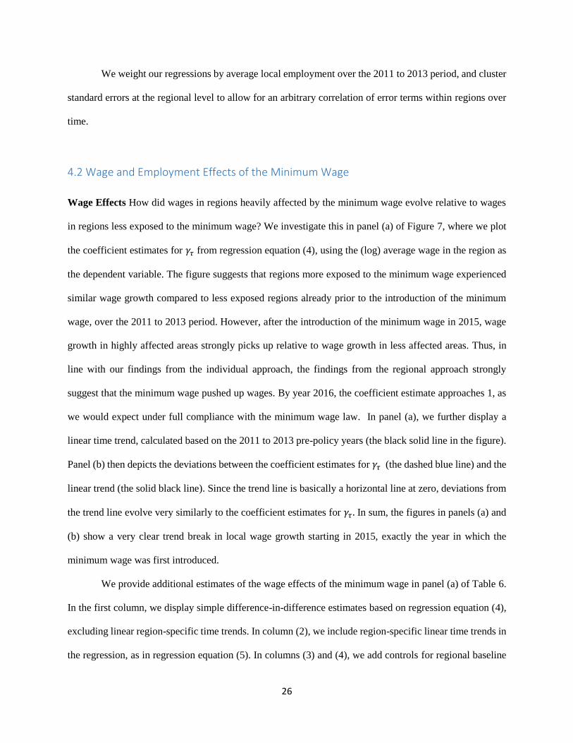
4.2 Wage and Employment Effects of the Minimum Wage

Wage Effects How did wages in regions heavily affected by the minimum wage evolve relative to wages

in regions less exposed to the minimum wage? We investigate this in panel (a) of Figure 7, where we plot

the coefficient estimates for 𝛾𝜏 from regression equation (4), using the (log) average wage in the region as

the dependent variable. The figure suggests that regions more exposed to the minimum wage experienced

similar wage growth compared to less exposed regions already prior to the introduction of the minimum

wage, over the 2011 to 2013 period. However, after the introduction of the minimum wage in 2015, wage

growth in highly affected areas strongly picks up relative to wage growth in less affected areas. Thus, in

line with our findings from the individual approach, the findings from the regional approach strongly

suggest that the minimum wage pushed up wages. By year 2016, the coefficient estimate approaches 1, as

we would expect under full compliance with the minimum wage law. In panel (a), we further display a

linear time trend, calculated based on the 2011 to 2013 pre-policy years (the black solid line in the figure).

Panel (b) then depicts the deviations between the coefficient estimates for 𝛾𝜏 (the dashed blue line) and the

linear trend (the solid black line). Since the trend line is basically a horizontal line at zero, deviations from

the trend line evolve very similarly to the coefficient estimates for 𝛾𝜏 . In sum, the figures in panels (a) and

(b) show a very clear trend break in local wage growth starting in 2015, exactly the year in which the

minimum wage was first introduced.

We provide additional estimates of the wage effects of the minimum wage in panel (a) of Table 6.

In the first column, we display simple difference-in-difference estimates based on regression equation (4),

excluding linear region-specific time trends. In column (2), we include region-specific linear time trends in

the regression, as in regression equation (5). In columns (3) and (4), we add controls for regional baseline

27

characteristics interacted with a linear time trend or with fully flexible year effects, rather than a region-

specific linear time trend. All specifications clearly indicate that the minimum wage raised wages. A one

percentage point increase in the gap measure leads to an increase in local wages by between 0.68% to

0.80%.

Employment Effects Panels (c) and (d) of Figure 7 and panel (b) in Table 6 provide a

corresponding analysis for the employment effects of the minimum wage. Panel (c) of Figure 7 illustrates

that local employment, measured as the number of workers employed in the region (in logs), fell at a nearly

linear rate in more exposed relative to less exposed areas throughout the entire 2011 to 2016 period.13 Panel

(d) depicts the deviations from the coefficient estimates 𝛾𝜏 (the blue dashed line in panel (c)) and the linear

trend (the black solid line in panel (c)), estimated for the pre-policy period 2011 to 2013 and updated for

the post-policy period. These deviations are all close to zero, suggesting that the minimum wage had no

discernable impact on local employment, in line with our findings from the individual analysis.

We report corresponding difference-in-difference estimates based on variants of regression

equation (5) in panel (b) of Table 6. In line with the evidence presented in the figure, the difference-in-

difference estimates indicate that the minimum wage did not reduce local employment, once we account in

various ways for differential pre-trends in employment (columns (2) to (4)). The estimate from our preferred

specification in the second column implies that that we can reject the hypothesis that employment in the

10% regions most exposed to the minimum wage (with a gap measure of 0.033) declined, relative to the

10% least exposed regions (with a gap measure of 0.009), by more than 1.5% ((0.018-1.96×0.059)×(0.033-

0.009) at a 5% confidence level. Putting it differently, the estimates for the local wage and employment

responses to the minimum wage presented in panels (a) and (b) rule an employment elasticity with respect

to wage that is larger (in absolute magnitude) than -0.14 at a 5% confidence level.14 The absence of a

13 The slope implies that the 10% regions most exposed to the minimum wage lost 4% of their employment relative

to the 10% regions least exposed to the minimum wage between 2011 and 2014. 14 Dividing estimates in panel (b) by estimates in panel (a) provides us with an estimate of the employment elasticity

with respect to the wage. We compute standard errors of this ratio through bootstrapping.

28

negative employment effect not only at the individual level, but also at the regional level further suggests

that employment prospects of unemployed workers are not substantially harmed by the introduction of the

minimum wage.

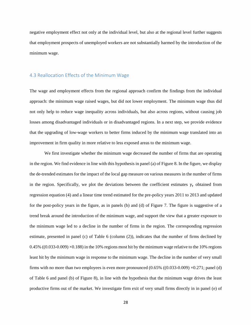
4.3 Reallocation Effects of the Minimum Wage

The wage and employment effects from the regional approach confirm the findings from the individual

approach: the minimum wage raised wages, but did not lower employment. The minimum wage thus did

not only help to reduce wage inequality across individuals, but also across regions, without causing job

losses among disadvantaged individuals or in disadvantaged regions. In a next step, we provide evidence

that the upgrading of low-wage workers to better firms induced by the minimum wage translated into an

improvement in firm quality in more relative to less exposed areas to the minimum wage.

We first investigate whether the minimum wage decreased the number of firms that are operating

in the region. We find evidence in line with this hypothesis in panel (a) of Figure 8. In the figure, we display

the de-trended estimates for the impact of the local gap measure on various measures in the number of firms

in the region. Specifically, we plot the deviations between the coefficient estimates 𝛾𝜏 obtained from

regression equation (4) and a linear time trend estimated for the pre-policy years 2011 to 2013 and updated

for the post-policy years in the figure, as in panels (b) and (d) of Figure 7. The figure is suggestive of a

trend break around the introduction of the minimum wage, and support the view that a greater exposure to

the minimum wage led to a decline in the number of firms in the region. The corresponding regression

estimate, presented in panel (c) of Table 6 (column (2)), indicates that the number of firms declined by

0.45% ((0.033-0.009) ×0.188) in the 10% regions most hit by the minimum wage relative to the 10% regions

least hit by the minimum wage in response to the minimum wage. The decline in the number of very small

firms with no more than two employees is even more pronounced (0.65% ((0.033-0.009) ×0.271; panel (d)

of Table 6 and panel (b) of Figure 8), in line with the hypothesis that the minimum wage drives the least

productive firms out of the market. We investigate firm exit of very small firms directly in in panel (e) of

29

Figure 8. The figure provides clear evidence of increased exit of small businesses after the introduction of

the minimum wage in regions heavily exposed to relative to regions barely hit by the minimum wage.

Since the minimum wage has little impact on overall local employment, the decline in the number

of firms induced by the minimum wage implies an increase in average firm size in the region, by 0.36% in

the 10% regions most exposed relative to the 10% regions least exposed to the minimum wage (panel (e)

of Table 6 and panel (c) of Figure 8). Panel (d) of Figure 8 further highlights that the minimum wage

increased the average firm wage premium, measured as a fixed firm effect in an AKM-style regression

estimated using only pre-policy data, in heavily exposed relative to barely exposed regions. The coefficient

estimates, reported in panels (a) and (g) in Table 7 (column (2)), imply that 18.2% (0.125/0.685) of the

overall increase in the local wage due to the introduction of the minimum wage can be attributed to the

reallocation of workers to firms that pay a higher wage premium.

To summarize, our findings from both the individual and regional approach highlight that the

minimum wage pushed up wages, but did not reduce employment. Both approaches further suggest that the

minimum wage led to reallocation effects: the minimum wage induced low-wage workers to move up to

better and larger firms; it further induced a shift away from micro firms toward larger firms, and toward

firms paying a higher wage premium, in regions where the minimum wage was more binding.

5 Discussion

There are three types of main models that could account for the patterns of reallocation, induced by the

minimum wage, observed in the data: models with search frictions; models of monopsonistic or

oligopolistic competition; and models with frictions in the product market. In all three types of models, a

minimum wage may not lead to employment losses, and may increase overall welfare in the economy.

Next, we highlight specific features in the data that are most easily explained by each one of the three model

types (but do not rule out the other two). Overall, we conclude that the minimum wage-induced reallocation

is unlikely to be driven by a single mechanism; rather, all three mechanisms are at play.

30

All three types of models predict that the minimum wage drives the least productive firms out of

business, as they are no longer profitable due to increased wage costs. Our finding of increased exits of

micro firms that employ no more than two employees in regions heavily affected relative to regions barely

hit by the minimum wage following the introduction of the minimum wage (panel (e) of Figure 8) is very

much consistent with this prediction.

Acemoglu (2001) provides an explanation for why a minimum wage may induce a shift toward

more productive, capital-intensive firms in the presence of search frictions. He argues that the creation of

capital-intensive jobs with high start-up costs inherently involves a “hold-up” problem, forcing the firm to

bargain to a higher wage. In consequence, firms create too many “bad” jobs (i.e., jobs with a low capital

intensity) and too few “good” jobs in the unregulated equilibrium. A minimum wage induces firms to

destroy some jobs with low capital intensity, and set up additional jobs with high capital intensity. While

we cannot directly measure capital intensity in the firm, we can proxy it with the firm wage fixed effect and

the share of high-skilled workers in the firm.15 Our findings that low-wage workers reallocated toward firms

with a higher firm fixed effect (panel (b) of Figure 4) and to skill-intensive firms (panel (b) in Figure 5) in

response to the minimum wage provides empirical support for the mechanisms described in Acemolgu

(2001).

Models of monopsonistic or oligopolistic competition provide an alternative explanation for the

minimum-wage induced reallocation of low-wage workers toward firms of higher quality (e.g., Manning,

2003 and Bhaskar, Manning, To 2002, Bergen, Herkenhoff, Mongey, 2019). In these types of models (and

similar to equilibrium models with search frictions), monopsony power allows firms to set wages below the

marginal product of labor and more productive firms find it optimal to set higher wages and employ more

workers. Card, Cardoso, Heinig and Kline (2018) argue that monopsony power of firms naturally emerges

when workers have idiosyncratic, non-pecuniary preferences to work at a particular firm. Possibly the most

15 Lochner et al. (2019) show a strong positive correlation between the firm wage fixed effect and the capital intensity

of the firm. Numerous papers provide evidence for the complementarity between capital and high-skilled workers

(e.g., Goldin and Katz, 1998).

31

important non-pecuniary characteristic of a particular job is the commuting time from home to the

workplace: workers are willing to accept lower wages if the workplace is closer to their home. As a result,

low paying firms are able to survive in equilibrium, by mostly attracting workers from their close

neighborhood. The introduction of the minimum wage may drive these firms out of business, and workers

may have to find jobs that farther from their home.

We explore the possibility that the reallocation of low-wage movers to higher paying firms comes

at the expense of increased commuting distance (computed as the distance between the centroids of the

municipalities of residence and work) in Table 7. We report, as in Tables 3 to 5, generalized difference-in-

difference estimates. The estimates suggest that commuting distance increased by 1.5km (or 8%) for low-

wage workers relative to high-wage workers after the introduction of the minimum wage. The increase in

commuting time induced by the minimum wage is considerably larger for men than for women, in line with

the hypothesis that women have a particularly strong preference to work close to home (e.g. Hanson and

Johnston, 1985; Caldwell and Danieli, 2019). Interestingly, the reallocation effects of low-wage workers

towards higher paying firms are also stronger for men than women (see Figure 9), as men are more willing

to trade off wages and commuting time. These findings suggest that part of the reallocation effects are

driven by the monopsony power of firms.

Finally, reallocation effects toward firms of higher quality can also be explained by frictions in the

consumer market, as explored in Luca and Luca (2018) and in Mayneris et al. (2014). Consider a model

where firms produce differentiated goods, differ in their productivity, and face fixed costs of production,

as in for example Melitz, 2003. In this type of model, a minimum wage, by pushing up labor costs, causes

the least productive firms to exit the market. Consumers who had previously purchased goods from these

firms will switch to products produced by more efficient firms, which increases the demand for labor in

these firms. In this case, we would expect the reallocation to take place predominantly within, rather than

between industries. Our findings in panel (b) of Table 5 are roughly in line with this implication, as about

68% of the overall reallocation occurs within 3-digit industries. We would further expect customers

switching products in response to the minimum wage to happen primarily among locally traded goods (that

32

is, in retail- and restaurant-related industries) where firms have some power to set product prices, rather

than among goods traded in the national or world market. Figure 9 provides support for this prediction: the

reallocation effect of low wage workers to higher paying firms is considerably more pronounced in the non-

tradable sector than in the tradable sector.16

In sum, the reallocation effects induced by the minimum wage are likely to be driven by all three

mechanisms—search frictions in the labor market, monopsony power, and frictions in the product market.

6 Conclusion

This paper investigates the labor marker responses to Germany’s first-time introduction of the

nation-wide minimum wage. We find that the minimum wage policy pushed up wages without lowering

employment. The lack of employment responses, however, masks some important structural shifts in the

economy: the minimum wage lead to reallocation of workers from smaller, lower paying firms to larger,

higher paying firms, and thereby helped to improve the quality of firms in the economy.

These findings speak against the existence of perfectly competitive labor and product markets

where a minimum wage unambiguously reduces national welfare. Rather, reallocation effects of the type

we uncover naturally emerge in the presence of labor market search frictions, monopsony power, or product

market frictions. Our findings suggest that all three forces are likely to play a role in explaining the

reallocation patterns observed in the data. The three types of models have in common that the employment

effects of the minimum wage may be small or even positive, due to some market imperfections or distortions

prior to the introduction of the minimum wage. A minimum wage could potentially reduce the detrimental

effects of the market imperfections or distortions, and may thus improve welfare in the economy.

16 When classifying industries into non-tradable and tradable, we follow Mian and Sufi (2014) and classify retail- and

restaurant-related industries as non-tradable, and industries listed in global trade data as tradable, as in their method

1. Our findings are similar when we classify industries as non-tradable and tradable using their method 2.

33

Yet, our results do not imply that there are no workers or customers who lost out because of the

minimum wage policy. The minimum wage caused some small businesses to exit the market. These firms

may have produced specific goods that were particularly liked by certain customers, who may now be

forced to switch to, according to their taste, an inferior alternative. Furthermore, the reallocation of low-

wage workers to higher paying firms came at the expense of increased commuting time, which might have

left some workers worse off despite earning a higher wage.

Establishing the existence of reallocation effects and quantifying its size, as we have done in this

paper, is an important first step to understand the welfare implications of minimum wages.

References

• Aaronson, D., French, E., Sorkin, I., & To, T. (2018). “Industry dynamics and the minimum wage:

a putty‐clay approach”. International Economic Review, 59(1), 51-84.

• Acemoglu, D. (2001). “Good jobs versus bad jobs”. Journal of Labor Economics, 19(1), 1-21.

• Ahlfeldt, G. M., Roth, D., & Seidel, T. (2018). “The regional effects of Germany’s national

minimum wage.” Economics Letters, 172, 127-130.

• Antonczyk, D., Fitzenberger, B., & Sommerfeld, K. (2010). “Rising wage inequality, the decline

of collective bargaining, and the gender wage gap”. Labour Economics, 17(5), 835-847.

• Bagger, J., & Lentz, R. (2018). “An empirical model of wage dispersion with sorting”. The Review

of Economic Studies, 86(1), 153-190.

• Berger, D. W., Herkenhoff, K. F., & Mongey, S. (2019). “Labor Market Power”. NBER working

paper No. w25719, National Bureau of Economic Research.

• Bhaskar V., Manning A., & To, T. (2002). “Oligopsony and monopsonistic competition in labor

markets”, Journal of Economic Perspectives, 16(2), 155-174.

• Brochu, P., & Green, D. A. (2013). “The impact of minimum wages on labour market transitions”.

The Economic Journal, 123(573), 1203-1235.

• Burdett, K., & Mortensen, D. T. (1998). “Wage differentials, employer size, and unemployment”.

International Economic Review, 39(2), 257-273.

• Cahuc, P., Postel‐Vinay, F., & Robin, J. M. (2006). “Wage bargaining with on‐the‐job search:

Theory and evidence”. Econometrica, 74(2), 323-364.

• Caldwell, S., & Danieli, O. (2018). “Outside options in the labor market”. Working paper, Harvard

University.

• Card, D. (1992). “Using Regional Variation in Wages to Measure the Effects of the Federal

Minimum Wage”. Industrial and Labor Relations Review, 46(1), 22-37.

• Card, D., Cardoso, A. R., Heining, J., & Kline, P. (2018). “Firms and labor market inequality:

Evidence and some theory”. Journal of Labor Economics, 36(S1), S13-S70.

34

• Card D., Heining J., & Kline, P. (2013). “Workplace heterogeneity and the rise of West German

wage inequality”. Quarterly Journal of Economics, 128(3), 967-1015.

• Card, D., & Krueger, B. (1994). “Minimum Wages and Employment: A Case Study of the Fast-

Food Industry in New Jersey and Pennsylvania”. The American Economic Review, 84(4), 772-793.

• Card D., & Krueger, A.B. (1995). “Myth and measurement: the new economics of the minimum

wage”. Princeton, NJ: Princeton University Press.

• Cardoso, A.R. & P. Portugal (2006). “Disentangling the Minimum Wage Puzzle: An Analysis of

Worker Accessions and Separations”. Journal of the European Economic Association, 4(5), 988-

1013.

• Cengiz, D., Dube, A., Lindner, A., & Zipperer, B. (2019). “The effect of minimum wages on low-

wage jobs: Evidence from the United States using a bunching estimator”. NBER working paper

No. w25434, National Bureau of Economic Research.

• Clemens, J., & Wither, M. (2019). “The minimum wage and the Great Recession: Evidence of

effects on the employment and income trajectories of low-skilled workers”. Journal of Public

Economics, 170, 53-67.

• Currie, J., & Fallick, B. C. (1996). “The minimum wage and the employment of youth: evidence

from the NLSY”. Journal of Human Resources, 31(2), 404-428.

• Destatis (2016). “4 Millionen Jobs vom Mindestlohn betroffen”, Statistisches Bundesamt press

release No. 121, April 06, 2016.

• Draca, M., Machin, S., & van Reenen, J. (2011). "Minimum wages and firm profitability",

American Economic Journal: Applied Economics, 3(1), 129-51.

• Dube, A., Lester, T. W. & Reich M. (2016). “Minimum Wage Shocks, Employment Flows, and

Labor Market Frictions” Journal of Labor Economics 34(3), 663-704.

• Dustmann C., Ludsteck J., & Schönberg, U. (2009). “Revisiting the German wage structure”,

Quarterly Journal of Economics, 124(2), 843-881.

• Edin, P. A., & Topel, R. (1997). “Wage policy and restructuring: the Swedish labor market since

1960”. In The welfare state in transition: Reforming the Swedish model (pp. 155-202). University

of Chicago Press.

• Erixon L. (2017). “Progressive supply-side economics: an explanation and update of the Rehn-

Meidner model”, Cambridge Journal of Economics, 42(3), 653–697.

• Fitzenberger, B., & Doerr, A. (2016). “Konzeptionelle Lehren aus der ersten Evaluationsrunde der

Branchenmindestlöhne in Deutschland”. Journal for Labour Market Research, 49(4), 329-347.

• Fitzenberger, B., Osikominu, A. & Völter, R. (2005). “Imputation Rules to Improve the Education

Variable in the IAB Employment Subsample”, Schmollers Jahrbuch: Journal of Applied Social

Science Studies, 126(3), 405-436.

• Flinn, C. J. (2006). “Minimum wage effects on labor market outcomes under search, matching, and

endogenous contact rates”. Econometrica, 74(4), 1013-1062.

• Flinn, C. J., (2011). “The minimum wage and labor market outcomes”, Cambridge, Massachusetts:

MIT Press.

• Goldin, C., & Katz, L. F. (1998). “The origins of technology-skill complementarity”. The Quarterly

Journal of Economics, 113(3), 693-732.

• Hanson, S., & Johnston, I. (1985). “Gender differences in work-trip length: explanations and

implications”. Urban Geography, 6(3), 193-219.

35

• Harasztosi, P. & Lindner, A. (2019). “Who pays for the minimum wage”, American Economic

Review, forthcoming.

• Kügler, A., Schönberg, U., & Schreiner, R. (2018). “Productivity growth, wage growth and

unions”. In: Proceedings of ECB Forum on Central Banking, June 20th 2018, (pp. 215-247).

European Central Bank, Frankfurt.

• Lester, R. A. (1960). “Employment effects of minimum wages”. ILR Review, 13(2), 254-264.

• Luca, D. L., & Luca, M. (2018). “Survival of the fittest: the impact of the minimum wage on firm

exit”. Harvard Business School NOM Unit Working Paper 17-088, Harvard Business School,

Boston.

• Manning, A. (2003). “The real thin theory: monopsony in modern labour markets”. Labour

Economics, 10(2), 105-131.

• Mayneris, F., Poncet, S., & Zhang, T. (2014). “The cleansing effect of minimum wage: minimum

wage rules, firm dynamics and aggregate productivity in China”, CEPII Working Papers 2014-16,

Centre d’Etudes Prospectives et d’Informations Internationales, Paris.

• Melitz, M. J., (2003). “The impact of trade on intra-industry reallocations and aggregate industry

productivity”, Econometrica, 71(6), 1695-1725.

• Mian, A., & Sufi, A. (2014). “What explains the 2007–2009 drop in employment?”. Econometrica,

82(6), 2197-2223.

• Neumark D., & Wascher, W. L. (2010). “Minimum Wages and Employment”, Cambridge,

Massachusetts: The MIT Press.

• OECD Statistics (2019). “Minimum relative to average wages of full-time workers”, Organization

for Economic Co-operation and Development, Paris.

• Rebitzer, J. B., & Taylor, L. J. (1995). “The consequences of minimum wage laws: some new

theoretical ideas”. Journal of Public Economics, 56(2), 245-255.

• Song, J., Price, D. J., Guvenen, F., Bloom, N., & Von Wachter, T. (2018). “Firming up inequality”.

The Quarterly Journal of Economics, 134(1), 1-50.

• Sorkin, I. (2018). “Ranking firms using revealed preference”. Quarterly Journal of Economics,

133(3), 1331-1393.

• vom Berge, P., Kaimer, S., Copestake, S., Eberle, J., Klosterhuber, W., Krüger, J., Trenkle, S., &

Zakrocki, V. (2016a). “Arbeitsmarktspiegel: Entwicklungen nach Einführung des Mindestlohns

(Ausgabe 1)”. IAB-Forschungsbericht, 01/2016, Institute for Employment Research, Nuremberg.

• vom Berge, P., Kaimer, S., Eberle, J., Klosterhuber, W., & Lehnert, C. (2016b).

“Machbarkeitsstudie zur Erstellung eines Arbeitsmarktmonitors Mindestlohn (MoMiLo)”. IAB-

Forschungsbericht, 03/2016, Institute for Employment Research, Nuremberg.

• vom Berge, P., Verbeek, H., Umkehrer, M., Fertig, M., & Bender, S., (2014). “Vorbereitende

Forschung für die zweite Evaluationsrunde Mindestlöhne: Erschließung neuer Datenquellen”.

FDZ-Methodenreport, 03/2014, Institute for Employment Research, Nuremberg.

4.5<Wt-2<8.5 8.5<Wt-2<12.50 12.50<Wt-2<20.50

in East Germany 0.300 0.260 0.166

not German citizen 0.129 0.107 0.067

Education

share low-skilled 0.219 0.138 0.075

share medium-skilled 0.712 0.798 0.827

share high-skilled 0.069 0.064 0.098

Age Structure

share less than 24 0.175 0.136 0.076

share 24-44 0.441 0.485 0.509

share 45 -59 0.384 0.379 0.415

Employment Status

unemployed in previous year 0.215 0.138 0.058

share full-time 0.324 0.582 0.729

share part-time 0.267 0.258 0.248

share marginally employed 0.410 0.160 0.023

Industry Structure

Agriculture; Mining 0.002 0.002 0.003

Manufacturing; Electricity; Waste Management 0.101 0.153 0.235

Construction; Wholesale and Retail 0.234 0.265 0.284

Transportation; Accomodation and Food Services 0.216 0.137 0.082

Information and Communication; Finance and Insurance; Real Estate 0.036 0.033 0.048

Professional Services; Administrative and Support Services 0.216 0.200 0.108

Public Administration; Education; Human Health 0.114 0.169 0.209

Arts, Entertainment; Other Services 0.081 0.042 0.031

Number of observations 1,234,689 2,187,715 3,776,430

Table 1: Which Individuals are Heavily Affected by the Minimum Wage?

Wage bin in 2013

Notes: The table compares individuals located at different parts of the hourly wage distribution in terms of location, education, age,

employment status, and industry affiliation in June 2013, 18 months prior to the introduction of the hourly minimum wage of 8.50 per

hour in January 2015.

Sources: Labor Market Mirror and Employee Histories of the Institute for Employment Research in Nuremberg (BeH), 2011-2013.

(1) (2) (3) (4) (5)

Wage bin in t-2 [4.5,8.5) [8.5,12.5) [12.5,20.5) (1) minus (3) (2) minus (3)

2014 vs 2016 0.067 0.023 0.006 0.061 0.016

(0.0006) (0.0003) (0.0001) (0.0006) (0.0003)

2012 vs 2014 (Placebo) 0.017 0.009 0.006 0.010 0.003

(0.0005) (0.0003) (0.0001) (0.0006) (0.0003)

Baseline Change (2011 vs 2013) 0.199 0.118 0.080

2014 vs 2016 0.118 0.047 0.012 0.107 0.036

(0.0010) (0.0005) (0.0002) (0.0010) (0.0005)

2012 vs 2014 (Placebo) 0.022 0.012 0.006 0.015 0.006

(0.0009) (0.0005) (0.0002) (0.0009) (0.0005)

Baseline Change (2011 vs 2013) 0.220 0.064 -0.002

2014 vs 2016 0.009 0.003 0.002 0.007 0.001

(0.0004) (0.0002) (0.0001) (0.0004) (0.0003)

2012 vs 2014 (Placebo) 0.003 0.000 0.001 0.002 -0.001

(0.0004) (0.0002) (0.0001) (0.0004) (0.0003)

Baseline Change (2011 vs 2013) -0.242 -0.184 -0.141

2014 vs 2016 0.034 0.018 0.006 0.029 0.013

(0.0004) (0.0002) (0.0001) (0.0004) (0.0003)

2012 vs 2014 (Placebo) 0.010 0.006 0.002 0.009 0.004

(0.0003) (0.0002) (0.0001) (0.0004) (0.0003)

Baseline Change (2011 vs 2013) -0.180 -0.193 -0.179

Notes: In panel (a), we report the excess hourly wage growth in the 2014 vs 2016 post-policy period and

the 2012 vs 2014 “placebo” period relative to the 2011 vs 2013 pre-policy period for three groups of

workers: workers who earned less than the minimum wage at baseline ([4.5, 8.5), column (1)), workers who

earn more but close to the minimum wage at baseline ([8.5, 12.50), column (2)), and workers who earn

more than 12.50 Euro at baseline (column (3)). Estimates refer to coefficients δwt in equation (2) in the

text, where workers are grouped into three bins only. Columns (4) and (5) report generalized difference-in-

difference estimates that compare the excess wage growth of workers who earn less or close to the

minimum wage at baseline with the excess wage growth of workers who earn more than 12.50 Euro at

baseline (i.e., estimates in columns (1) and (2) minus estimates in column (3)). In panel (b), we repeat the

analysis, but now use the change in daily wages as the dependent variable. In both panels (a) and (b), the

sample is restricted to individuals who are employed both in period t-2 and t. In panel (c), we report

corresponding estimates using employment (1 if the individual is employed, 0 otherwise) as the dependent

variable. In panel (d), we instead use the change in full-time equivalents, where we assig a value of 1 if the

worker is employed full-time, 0.5 if the worker is employed part-time, 0.2 if the worker is marginally

employed, and 0 if the worker is not employed, as the dependent variable. All regressions control for

individual characteristics at baseline (age, education, sex, nationality, location fixed effects and industry

fixed effects).

Sources: Labor Market Mirror and Employee Histories of the Institute for Employment Research in

Nuremberg (BeH), 2011-2016.

Table 2: Effect of the Minimum Wage on Wages and Employment: Individual Approach

Panel (a): Hourly Wages

Panel (c): Employment (1 if employed)

Panel (d): Employment, full-time equivalents

Changes relative to 2011 vs 2013 Generalised difference-in-

difference

Panel (b): Daily Wages

(1) (2) (3) (4)

Wage bin in t-2 [4.5,8.5) [8.5,12.5) [4.5,8.5) [8.5,12.5)

Estimated effect 0.107 0.036 0.015 0.006

(0.0010) (0.0005) (0.0009) (0.0005)

Estimated effect 0.025 0.008 0.004 0.001

(0.0007) (0.0004) (0.0007) (0.0003)

Fraction attributable to reallocation 23.4%

Estimated effect 0.061 0.016 0.010 0.003

(0.0006) (0.0003) (0.0006) (0.0003)

Estimated effect: 0.005 0.001 0.001 0.000

(0.0003) (0.0002) (0.0003) (0.0002)

Fraction attributable to reallocation 8.2%

Estimated effect 0.004 0.001 0.000 0.000

(0.0003) (0.0001) (0.0003) (0.0001)

Fraction attributable to reallocation 6.6%

Panel (d): Firm's Wage Premium

Panel (e): Firm's Fixed Effect

Table 3: Reallocation to Higher Paying Firms: Individual Approach

Notes: The table investigates the effect of the minimum wage on the reallocation of low-wage workers to firms

that pay higher wages. Firm quality is measured before the minimum wage came into effect, and only changes

for workers who switch firms. In panel (b), we use the change in the firm’s average daily wage as the dependent

variable. In panel (d), firm quality is measured as the firm’s wage premium conditional on worker demographics

and employment status, calculated as the residual from an individual daily wage regression that controls for

workers’ full-time and part-time status in addition to worker age, skill and foreign status and is aggregated to

the firm level. In panel (e), the dependent variable is the firm’s fixed effect, obtained from an individual daily

wage regression for full-time workers that controls for worker age and worker, firm and year fixed effects and is

estimated for over a 7-year period prior to the implementation of the minimum wage (2008 to 2014). The table

reports generalised difference-in-difference estimates for the 2014 vs 2016 post-policy period (columns (1) and

(2)) and the 2012 vs 2014 “placebo” pre-policy period (columns (3) and (4)). These estimates compare the

excess improvement in firm quality (relative to the 2011 vs 2013 pre-policy period) of workers who earn less

than ([4.5, 8.5)), or close to ([8.5, 12.50) the minimum wage at baseline with the excess improvement in firm

quality of workers who earn more than 12.50 Euro at baseline, as in columns (4) and (5) in Table 2. For

comparison, we also report estimates using the change in the individual daily wage (panel (a); compare columns

(4) and (5) in panel (b) of Table 2) and the change in individual hourly wage (panel (c); compare columns (4) and

(5) in panel (a) of Table 2) as dependent variables. The table further reports the fraction of the overall

improvement in daily or hourly wages that can be attributed to the reallocation of workers to better firms in

bold. All regressions control for individual characteristics at baseline (age, education, sex, nationality, location

fixed effects and industry fixed effects).

Sources: Labor Market Mirror and Employee Histories of the Institute for Employment Research in

Nuremberg (BEH), 2011-2016, 20% random sample of individuals.

Main Effects (2014 vs 2016) Placebo Effects (2012 vs 2014)

(Generalized Difference-in-Difference Estimates)

Panel (a): Daily Wages

Panel (b): Firm's Average Daily Wage

Panel (c): Hourly Wages

(1) (2) (3) (4)

Wage bin in t-2 [4.5,8.5) [8.5,12.5) [4.5,8.5) [8.5,12.5)

Estimated effect 0.003 0.001 0.001 0.000

(0.0001) (0.0001) (0.0001) (0.0001)

Estimated effect 0.010 0.003 0.002 0.001

(0.0003) (0.0002) (0.0003) (0.0002)

Estimated effect -0.008 -0.003 -0.001 -0.001

(0.0003) (0.0001) (0.0002) (0.0001)

Estimated effect 0.043 0.015 0.012 0.004

(0.0021) (0.0013) (0.0019) (0.0013)

Panel (e): Firm's Churning Rate

Estimated effect -0.009 -0.003 0.001 0.002

(0.0005) (0.0003) (0.0004) (0.0003)

Panel (f): Firm's Poaching Index

Estimated effect 0.005 0.003 0.001 0.000

(0.0003) (0.0002) (0.0002) (0.0002)

Main Effects (2014 vs 2016) Placebo Effects (2012 vs 2014)

Table 4: Reallocation to Firms of Higher Quality

(Generalized Difference-in-Difference Estimates)

Panel (a): Firm's High Skilled Employment Share

Notes: The table investigates the effect of the minimum wage on the reallocation of low-wage

workers to firms of higher quality. Firm quality is measured before the minimum wage came into

effect, and only changes for workers who switch firms. In panels (a) to (c), we use changes in the

share of high-skilled workers (i.e., workers with a university education), full-time workers, and

marginally employed workers as dependent variables. In panel (d), firm quality is measured as firm

size (i.e., (log) number of employees in full-time equivalents). In panel (e), the dependent variable

is the change in firm’s churning rate, measured as the sum of workers who leave and join the firm,

divided by the number of employees at baseline. The dependent variable in panel (f) is the change

in the firm’s poaching index, computed as share of new hires that come from employment rather

than unemployment. The table reports generalised difference-in-difference estimates for the 2014

vs 2016 post-policy period (columns (1) and (2)) and the 2012 vs 2014 “placebo” pre-policy period

(columns (3) and (4)). These estimates compare the excess improvement in firm quality (relative to

the 2011 vs 2013 pre-policy period) of workers who earn less than ([4.5, 8.5)), or close to ([8.5,

12.50) the minimum wage at baseline with the excess improvement in firm quality of workers who

earn more than 12.50 Euro at baseline, as in columns (4) and (5) in Table 2. All regressions control

for individual characteristics at baseline (age, education, sex, nationality, location fixed effects and

industry fixed effects).Sources: Labor Market Mirror and Employee Histories of the Institute for Employment Research in

Nuremberg (BEH), 2011-2016, 20% random sample of individuals.

Panel (b): Firm's Full-time Employment Share

Panel (c): Firm's Marginal Employment Share

Panel (d): Firm Size

(1) (2) (3) (4)

Wage bin in t-2 [4.5,8.5) [8.5,12.5) [4.5,8.5) [8.5,12.5)

Estimated effect -0.0002 -0.0001 -0.0001 0.0000

(0.00005) (0.00003) (0.00005) (0.00003)

Estimated effect 0.0078 0.0003 0.0011 -0.0014

(0.0004) (0.0002) (0.0003) (0.0002)

Estimated effect 0.0019 0.0088 -0.0013 0.0020

(0.0006) (0.0005) (0.0006) (0.0005)

Estimated effect -0.0011 -0.0012 -0.0009 -0.0007

(0.0003) (0.0002) (0.0003) (0.0002)

Notes: The table investigates three potential channels through which the minimum wage-induced reallocation of low-

wage workers to firms of higher quality may occur. In panel (a), we investigate whether low-wage workers reallocate

to regions that pay higher wages following the introduction of the minimum wage. The dependent variable here is the

change in the (log) average daily wage in the region, measured prior to the introduction of the minimum wage. In

panel (b), we use the change in the (log) daily wage in the (3-digit) industry as the dependent variable to examine

whether low-wage workers move to higher paying industries in response to the minimum wage. In panel (c), we

investigate whether the minimum wage increased the probability that low-wage workers leave their baseline firm; the

dependent variable here is equal to 1 if the worker is employed in the same firm in period t as in period t-2, and 0

otherwise. In panel (d) we scrutinize whether the probability of moving to a newly born firm is affected by the

minimum wage. In all three panels, the sample is restricted to workers who are employed both at baseline (t-2) and in

period t. The table reports generalised difference-in-difference estimates for the 2014 vs 2016 post-policy period

(columns (1) and (2)) and the 2012 vs 2014 “placebo” pre-policy period (columns (3) and (4)). These estimates

compare the excess improvement in firm quality (relative to the 2011 vs 2013 pre-policy period) of workers who earn

less than ([4.5, 8.5)), or close to ([8.5, 12.50) the minimum wage at baseline with the excess improvement in firm

quality of workers who earn more than 12.50 Euro at baseline, as in columns (4) and (5) in Table 2. All regressions

control for individual characteristics at baseline (age, education, sex, nationality, location fixed effects and industry

fixed effects).Sources: Labor Market Mirror and Employee Histories of the Institute for Employment Research in Nuremberg (BEH),

2011-2016, 20% random sample of individuals.

Table 5: Reallocation to Higher Paying Regions and Industries?

(Generalized Difference-in-Difference Estimates)

Main Effects (2014 vs 2016) Placebo Effects (2012 vs 2014)

Panel (a): Average Daily Wage in the Region

Panel (b): Average Daily Wage in the Industry (3-digit)

Panel (c): Probability of Switching Firms

Panel (d): Probability of Switching to a Firm that Born after (t-2)

(1) (2) (3) (4)

Panel (a): Hourly Wages

0.795 0.685 0.754 0.798

(0.0402) (0.0527) (0.0500) (0.0861)

-1.513 0.0176 0.131 0.375

(0.127) (0.0594) (0.0910) (0.153)

Reallocation Effects: Improvement in Firm Quality in the Region

Panel (c): Number of firms

-1.458 -0.188 -0.216 -0.243

(0.107) (0.0384) (0.0631) (0.104)

-1.479 -0.271 -0.318 -0.35

(0.0976) (0.0901) (0.101) (0.163)

Panel (e): Average firm size

-0.0428 0.154 0.22 0.307

(0.0607) (0.0563) (0.0719) (0.105)

0.414 0.125 0.208 0.282

(0.0297) (0.0304) (0.0307) (0.0483)

Location fixed effects yes yes yes yes

Year fixed effects yes yes yes yes

Location specific linear time trends no yes no no

Local baseline characteristics interacted with year fixed effects no no no yes

Sources: Labor Market Mirror and Employee Histories of the Institute for Employment Research in Nuremberg (BEH), 2011-2016,

aggregated across regions (401 counties) and years.

Table 6: Wage, Employment and Reallocation Effects of the Minimum Wage: Regional Approach

Panel (b): Employment (Number of Workers)

Notes: In column (1) of the table, we report difference-in-difference estimates for the impact of the region’s exposure to the minimum

wage, measured as the average gap measure for the 2011 to 2013 pre-policy years as (equation (3)), on the (log) mean hourly wage in the

region (panel (a)); (log) employment in the region ((log) number of workers), panel (b)); the number of firms in the region (panel (c));the

number of micro firms with 1 or 2 employees in the region (panel (d)); average firm size in the region (panel (e)); the average firm fixed

effect in the region (obtained from an AKM style regression estimated over the pre-policy period, panel (f)). Estimates are based on

regression equation (4) and do not include controls for possibly divergent pre-trends in regions heavily and barely affected by the minimum

wage. In columns (2) to (4), we account for such differential pre-trends by including, as in regression equation (5), a region-specific linear

time trend (column (2)); by including baseline regional characteristics interacted with a linear time trend (column (3)); or by including

baseline regional characteristics interacted with fully flexible year fixed effects (column (4)). Regressions are weighted by local employment

averaged over the 2011 to 2013 pre-policy period. Standard errors are clustered at the regional level.

Panel (f): Average Firm FEs

Local baseline characteristics interacted with linear

time trendno yes nono

No controls for

differential pre-trends Controls for differential pre-trends

Panel (d): Number Micro Firms (1-2 workers)

(1) (2) (3) (4)

Wage bin in t-2 [4.5,8.5) [8.5,12.5) [4.5,8.5) [8.5,12.5)

Estimated Effect 1.868 0.559 0.518 -0.050

(0.0972) (0.0811) (0.0897) (0.0790)

Men 3.406 0.578 1.037 -0.106

(0.1801) (0.1336) (0.1632) (0.1292)

Women 0.866 0.414 0.094 -0.085

(0.1136) (0.0977) (0.1056) (0.0953)

Panel (a): Driving Distance

Table 7: Effect of the Minimum Wage on Commuting Distance

Sources: Labor Market Mirror and Employee Histories of the Institute for Employment Research in

Nuremberg (BEH), 2011-2016, 20% random sample of individuals.

Notes: In panel (a) of the table, we investigate whether the reallocation of low-wage workers to better

firms in response to the minimum wage comes at the expense of increased commuting distance. The

dependent variable is the change in the driving distance in kilometres between the centre of the

municipality of residence and the municipality of work. In panel (b), we examine whether the change in

commuting distance differs for men or women. The table reports generalised difference-in-difference

estimates for the 2014 vs 2016 post-policy period (columns (1) and (2)) and the 2012 vs 2014 “placebo”

pre-policy period (columns (3) and (4)). These estimates compare the change in driving distance (relative

to the 2011 vs 2013 pre-policy period) for workers who earn less than ([4.5, 8.5)), or close to ([8.5,

12.50) the minimum wage at baseline with the change in driving distance for workers who earn more

than 12.50 Euro at baseline, as in columns (4) and (5) in Table 2. All regressions control for individual

characteristics at baseline (age, education, sex, nationality, location fixed effects and industry fixed

effects).

Main Effects (2014 vs 2016) Placebo Effects (2012 vs 2014)

(Generalized Difference-in-Difference Estimates)

Panel (b): Driving Distance - Men vs Women

(1) (2) (3) (4) (5) (6)

Wage bin in t-2 [4.5,8.5) [4.5,8.5) [4.5,8.5) [4.5,8.5) [4.5,8.5) [4.5,8.5)

Panel (a): Hourly Wages

2014 vs 2016 0.058 0.060 0.061 0.060 0.061 0.058

(0.0006) (0.0006) (0.0006) (0.0006) (0.0006) (0.0006)

2012 vs 2014 (Placebo) 0.009 0.010 0.010 0.010 0.010 0.009

(0.0006) (0.0006) (0.0006) (0.0006) (0.0006) (0.0006)

2014 vs 2016 0.004 0.008 0.007 0.009 0.007 0.007

(0.0005) (0.0004) (0.0004) (0.0004) (0.0004) (0.0004)

2012 vs 2014 (Placebo) 0.001 0.002 0.002 0.002 0.002 0.002

(0.0005) (0.0004) (0.0004) (0.0004) (0.0004) (0.0004)

Panel (c): Firm's Average Daily Wage

2014 vs 2016 0.022 0.023 0.025 0.022 0.025 0.022

(0.0008) (0.0007) (0.0007) (0.0007) (0.0007) (0.0007)

2012 vs 2014 (Placebo) 0.003 0.003 0.004 0.003 0.004 0.003

(0.0007) (0.0007) (0.0007) (0.0007) (0.0007) (0.0007)

Demographic Controls no yes yes yes yes yes

Industry FEs no no yes no yes yes

Location FEs no no no yes yes yes

District UR X wage bin no no no no no yes

Sources: Labor Market Mirror and Employee Histories of the Institute for Employment Research in Nuremberg (BEH),

2011-2016, 20% random sample of individuals.

Panel (b): Employment (1 if Employed)

Table A1: Wage, Employment and Reallocation Effects of the Minimum Wage: Robustness Checks

Notes: The table shows the robustness of our key results with respect to the inclusion of additional control variables

measured at baseline. The table shows, for workers earning less than the minimum wage, hourly wage growth (panel

(a)), the probability of remaining employed (panel (b)), the change in the firm’s (log) average daily wage (panel (c)),

and the change in firm size (panel (d)) relative to the 2011 vs 2013 period, as in column (1) of Table 2. In column (1),

we do not include any baseline controls. In column (2), we add demographic controls (education, age and foreign

status). In column (3), we include industry affiliation in addition to demographic controls in the regression, as in our

baseline specification. In column (4), we control for location instead of industry affiliation. In column (5), we control

for both demographic characteristics, industry affiliation and location. In column (6), we further add the regional

unemployment rate interacted with wage bins as a control, to account for potential business cycle effects that

differentially affect workers at different parts of the wage distribution.

Panel (b): Unemployment Rate

Notes: The figure provides an overview of the macroeconomic conditions at the time of the introduction of the minimum wage in January 2015. Panel (a)

shows nominal GDP growth; panel (b) shows the unemployment rate, and panel (c) shows total employment between 2011 and 2016.

Source: : DeStatis, 2011-2016.

Figure 1: Macroeconomic Conditions, 2011 to 2016

Panel (a) Noimnal GDP

Panel (c): Employment

(b) Two-Year Hourly Wage Growth by Initial Wage Bin, relative to 2011 vs 2013

Notes: In panel (a), we plot two-year hourly wage growth of individuals who were employed in t-

2 and t against their initial wage bin, separately for the periods 2011 vs 2013 (green line) to 2014

vs 2016 (black line), while controlling for individual characteristics at baseline (age, education,

sex, county and industry fixed effects). Estimates refer to coefficients γwt in regression equation

(1) in the text. In panel (b), we plot two-year wage growth by initial wage bin in the periods 2012

vs 2014 to 2014 vs 2016 relative to the 2011 vs 2013 pre-policy period, once again controlling for

individual characteristics at baseline. Estimates refer to coefficients δwt in regression equation

(2), and correspond to the differences between the black, blue, and red lines and the green line in

panel (a). The black vertical line indicates the minimum wage of 8.50 Euro per hour.

Sources: Labor Market Mirror and Employee Histories of the Institute for Employment Research

in Nuremberg (BEH), 2011-2016, 20% random sample of individuals.

(a) Two-Year Hourly Wage Growth by Initial Wage Bin

Figure 2: Wage Effects of the Minimum Wage: Individual Approach

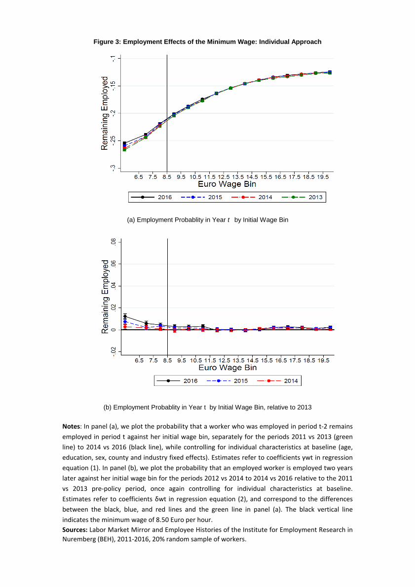
Sources: Labor Market Mirror and Employee Histories of the Institute for Employment Research in

Nuremberg (BEH), 2011-2016, 20% random sample of workers.

Figure 3: Employment Effects of the Minimum Wage: Individual Approach

(a) Employment Probablity in Year t by Initial Wage Bin

(b) Employment Probablity in Year t by Initial Wage Bin, relative to 2013

Notes: In panel (a), we plot the probability that a worker who was employed in period t-2 remains

employed in period t against her initial wage bin, separately for the periods 2011 vs 2013 (green

line) to 2014 vs 2016 (black line), while controlling for individual characteristics at baseline (age,

education, sex, county and industry fixed effects). Estimates refer to coefficients γwt in regression

equation (1). In panel (b), we plot the probability that an employed worker is employed two years

later against her initial wage bin for the periods 2012 vs 2014 to 2014 vs 2016 relative to the 2011

vs 2013 pre-policy period, once again controlling for individual characteristics at baseline.

Estimates refer to coefficients δwt in regression equation (2), and correspond to the differences

between the black, blue, and red lines and the green line in panel (a). The black vertical line

indicates the minimum wage of 8.50 Euro per hour.

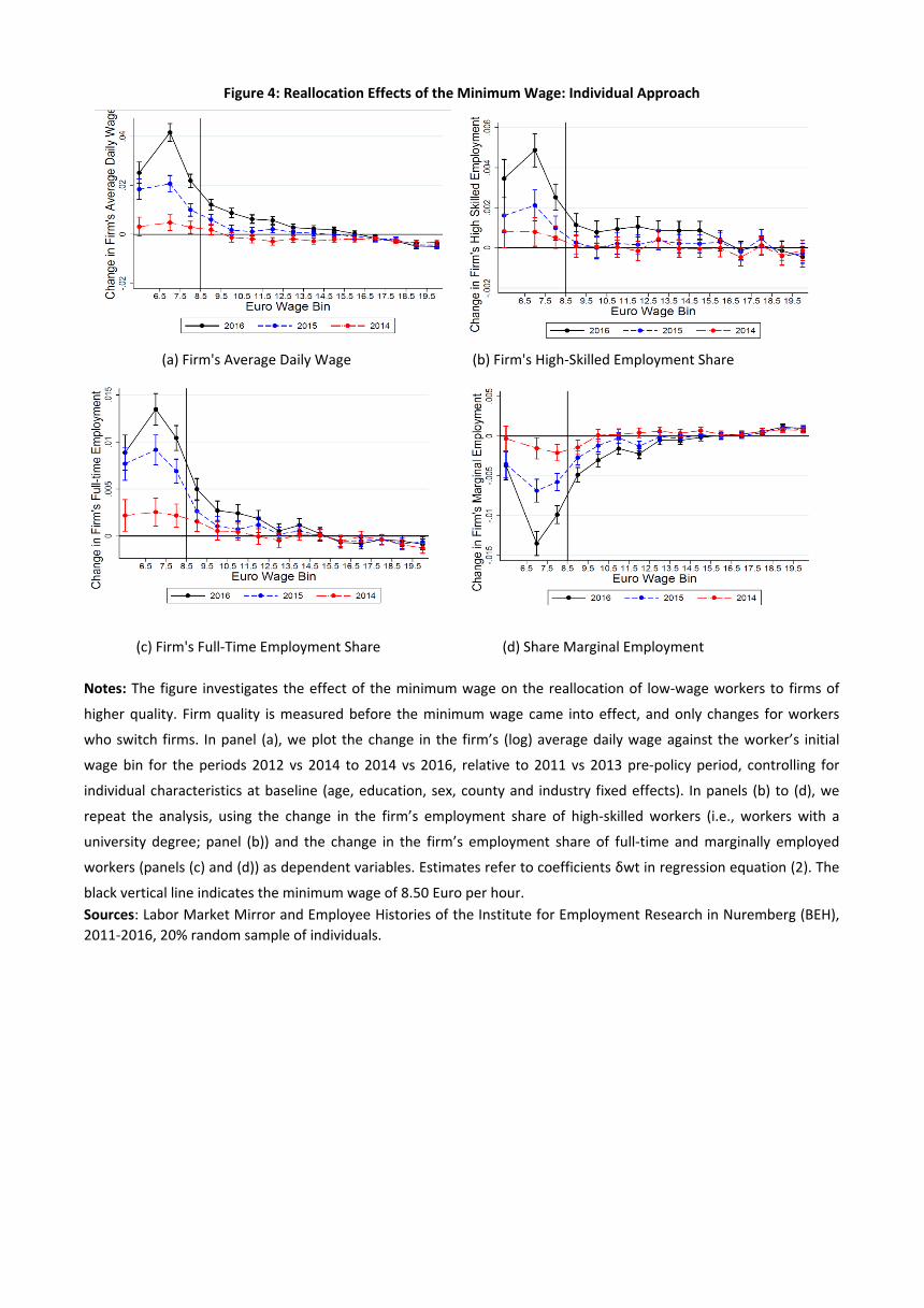
Notes: The figure investigates the effect of the minimum wage on the reallocation of low-wage workers to firms of

higher quality. Firm quality is measured before the minimum wage came into effect, and only changes for workers

who switch firms. In panel (a), we plot the change in the firm’s (log) average daily wage against the worker’s initial

wage bin for the periods 2012 vs 2014 to 2014 vs 2016, relative to 2011 vs 2013 pre-policy period, controlling for

individual characteristics at baseline (age, education, sex, county and industry fixed effects). In panels (b) to (d), we

repeat the analysis, using the change in the firm’s employment share of high-skilled workers (i.e., workers with a

university degree; panel (b)) and the change in the firm’s employment share of full-time and marginally employed

workers (panels (c) and (d)) as dependent variables. Estimates refer to coefficients δwt in regression equation (2). The

black vertical line indicates the minimum wage of 8.50 Euro per hour.

Sources: Labor Market Mirror and Employee Histories of the Institute for Employment Research in Nuremberg (BEH),

2011-2016, 20% random sample of individuals.

(a) Firm's Average Daily Wage

(c) Firm's Full-Time Employment Share

(b) Firm's High-Skilled Employment Share

(d) Share Marginal Employment

Figure 4: Reallocation Effects of the Minimum Wage: Individual Approach

Notes: In the figure, we plot the change in firm quality between periods t-2 and t for workers who are employed in

both periods against their initial wage bin for the periods 2012 vs 2014 to 2014 vs 2016, relative to the 2011 vs 2013

pre-policy period. Regressions control for individual characteristics at baseline (age, education, sex, county and

industry fixed effects). Estimates refer to coefficients δwt in regression equation (2). Firm quality is measured before

the minimum wage came into effect, and only changes for workers who switch firms. In panel (a), firm quality is

measured as the firm’s wage premium, calculated as the average wage residual in the firm obtained from an individual

wage regression that controls for workers’ demographic characteristics (age, sex, foreign status and education) and

workers’ employment status (full-time, part-time, marginal employment). In panel (b), firm quality is measured as the

firm’s fixed effect, estimated in an AKM-style wage regression that controls for worker and firm effects over a 7-year

pre-policy window. In panel (c), we use firm size as a measure for firm quality. In panel (d), the dependent variable is

the change in the firm’s churning rate, calculated as the sum of workers who leave and join the firm, divided by the

number of employees at baseline. The black vertical line indicates the minimum wage of 8.50 Euro per hour.

Sources: Labor Market Mirror and Employee Histories of the Institute for Employment Research in Nuremberg (BEH),

2011-2016, 20% random sample of workers.

(a) Firm's Wage Premium

(c) Firm Size

(b) Firm's Fixed Effect

(d) Firm's Churning Rate

Figure 5: Reallocation Effects of the Minimum Wage: Individual Approach

Figure 5: Exposure to the Minimum Wage across Regions

Notes: The figure shows the exposure to the minimum wage across 401 regions

(districts). Regional exposure to the minimum wage is measured using the gap

measure, as in equation (1).

Sources: Labor Market Mirror and Employee Histories of the Institute for Employment

Research in Nuremberg (BEH), 2011-2013.

Sources: Labor Market Mirror and Employee Histories of the Institute for Employment Research in Nuremberg (BEH), 2011-2016,

aggregated across regions (401 counties) and years.

(c) Employment (d) De-trended Employment

Figure 7 : Wage and Employment Effects of the Minimum Wage: Regional Approach

(a) Hourly Wages (b) De-trended Hourly Wages

Notes: Panels (a) and (c) trace out how (log) local hourly wages (panel (a)) and (log) local employment (the number of employed

workers in the region, panel (c)) evolve in regions differentially exposed to the minimum wage, relative to the pre-policy year 2013

(the dashed blue line). Plotted effects refer to coefficients γτ in regression equation (4). The figures also plot a linear time trend

estimated for the 2011-2013 pre-policy years and then updated for later years (the solid black line). Panels (b) and (d) display the

deviations between the coefficient estimates and the linear time trend.

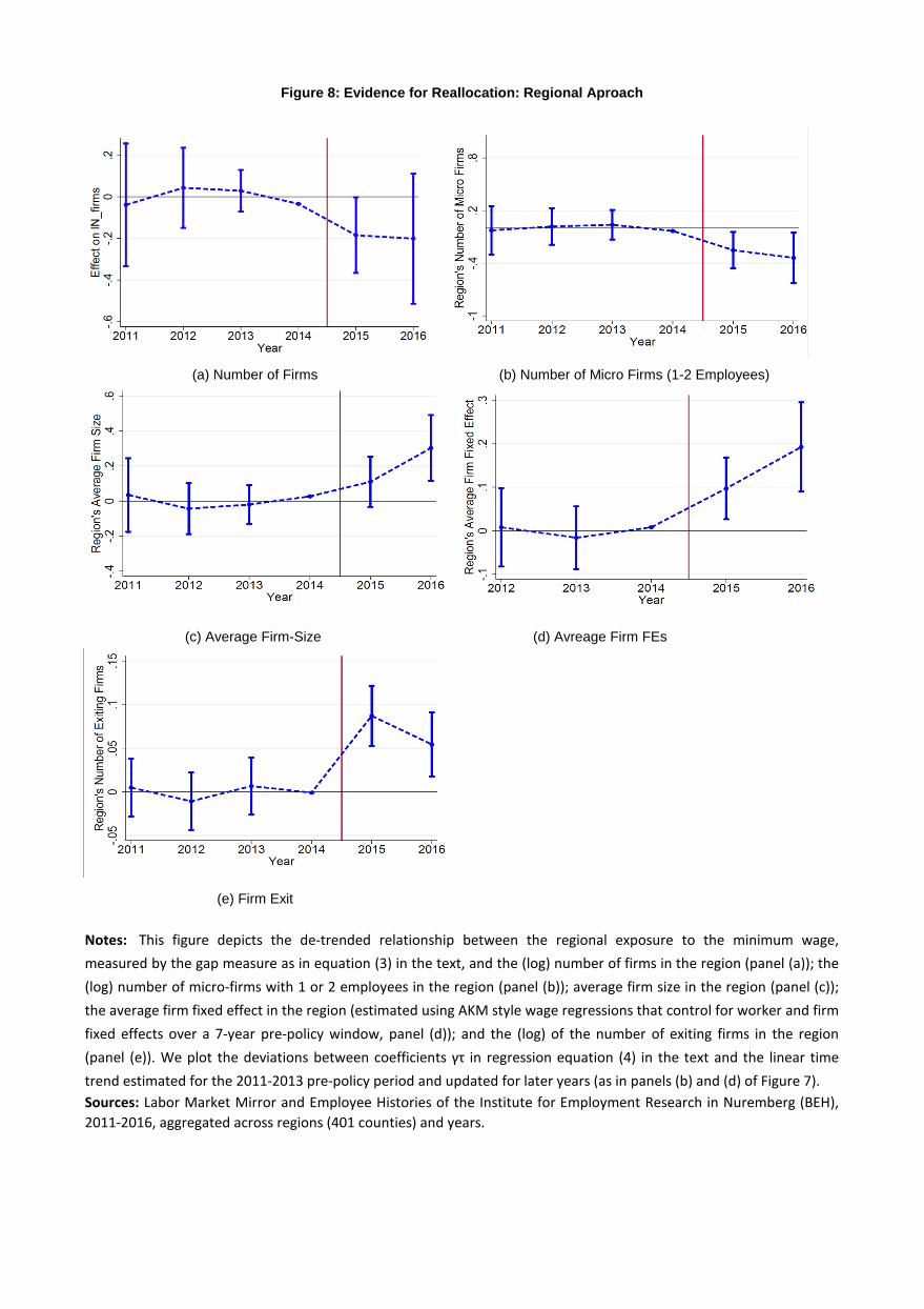
Notes: This figure depicts the de-trended relationship between the regional exposure to the minimum wage,

measured by the gap measure as in equation (3) in the text, and the (log) number of firms in the region (panel (a)); the

(log) number of micro-firms with 1 or 2 employees in the region (panel (b)); average firm size in the region (panel (c));

the average firm fixed effect in the region (estimated using AKM style wage regressions that control for worker and firm

fixed effects over a 7-year pre-policy window, panel (d)); and the (log) of the number of exiting firms in the region

(panel (e)). We plot the deviations between coefficients γτ in regression equation (4) in the text and the linear time

trend estimated for the 2011-2013 pre-policy period and updated for later years (as in panels (b) and (d) of Figure 7).

Sources: Labor Market Mirror and Employee Histories of the Institute for Employment Research in Nuremberg (BEH),

2011-2016, aggregated across regions (401 counties) and years.

(e) Firm Exit

(a) Number of Firms

(c) Average Firm-Size (d) Avreage Firm FEs

(b) Number of Micro Firms (1-2 Employees)

Figure 8: Evidence for Reallocation: Regional Aproach

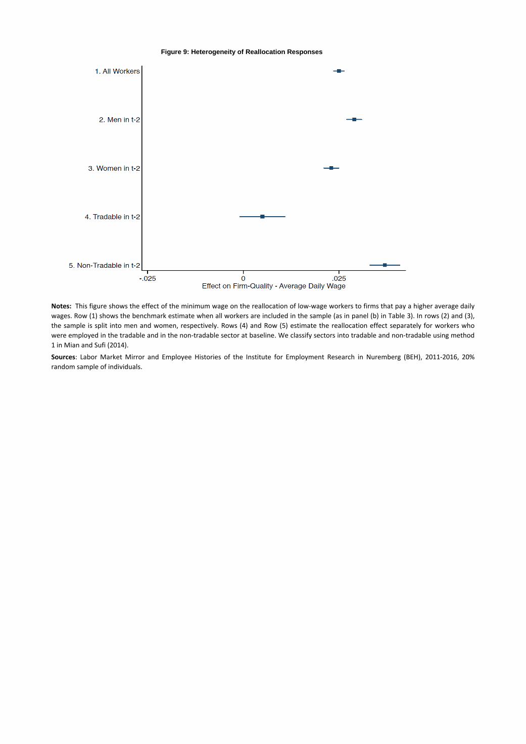
Figure 9: Heterogeneity of Reallocation Responses

Notes: This figure shows the effect of the minimum wage on the reallocation of low-wage workers to firms that pay a higher average daily

wages. Row (1) shows the benchmark estimate when all workers are included in the sample (as in panel (b) in Table 3). In rows (2) and (3),

the sample is split into men and women, respectively. Rows (4) and Row (5) estimate the reallocation effect separately for workers who

were employed in the tradable and in the non-tradable sector at baseline. We classify sectors into tradable and non-tradable using method

1 in Mian and Sufi (2014).

Sources: Labor Market Mirror and Employee Histories of the Institute for Employment Research in Nuremberg (BEH), 2011-2016, 20%

random sample of individuals.