Realized Laplace Transforms for Estimation of Jump Diffusive

Volatility Models∗

Viktor Todorov† George Tauchen ‡§ Iaryna Grynkiv ¶

June 12, 2011

Abstract

We develop an efficient and analytically tractable method for estimation of parametric volatil-ity models that is robust to price-level jumps. The method entails first integrating intra-daydata into the Realized Laplace Transform of volatility, which is model-free estimate of dailyintegrated empirical Laplace transform of the unobservable volatility. The estimation then isdone by matching moments of the integrated joint Laplace transform with those implied by theparametric volatility model. In the empirical application, the best fitting volatility model isa non-diffusive two-factor model where low activity jumps drive its persistent component andmore active jumps drive the transient one.

Keywords: Jumps, High-Frequency Data, Laplace Transform, Stochastic Volatility Models.

JEL classification: C51, C52, G12.

∗We would like to thank the editor, an Associate Editor, a referee as well as Torben Andersen, Tim Bollerslev,Andrew Patton, and many conference and seminar participants for numerous suggestions and comments. Todorov’swork was partially supported by NSF grant SES-0957330.

†Department of Finance, Kellogg School of Management, Northwestern University, Evanston, IL 60208; e-mail:v-todorov@northwestern.edu

‡Department of Economics, Duke University, Durham, NC 27708; e-mail: george.tauchen@duke.edu.§corresponding author¶Department of Economics, Duke University, Durham, NC 27708; e-maail: ig9@duke.edu.

1 Introduction

Stochastic volatility and price-level jumps are two well-recognized features of asset price dynamics

that differ in economically significant ways. Given the substantial compensations for these two

risks demanded by investors, as evident from option prices, it is of central importance to better

understand their dynamic characteristics. When using coarser sampling of stock prices such as

daily data, the separation of volatility from price-level jumps becomes relatively difficult, and,

most important, it depends crucially on the correct modeling of all aspects in the asset model;

misspecification of any one feature of the model for the asset dynamics can lead to erroneous

evidence about the role and significance of each of those risks. On the other hand, the availability

of high-frequency data provides a model-free way of disentangling the key features of the price

dynamics.

Price level jumps have recently been studied very extensively.1 There is substantial parametric

and non-parametric evidence for rare, but very sharp price movements, as would be expected from a

compound Poisson process. There is also some evidence for smaller, more vibrant price-level jumps,

as predicted by models built on Levy processes with so-called Blumenthal-Getoor indexes above

zero.2 This evidence is documented by Ait-Sahalia and Jacod (2009a, 2010) for liquid individual

equity prices, by Todorov and Tauchen (2010b) for index options prices, see also the references

therein.

The aim of this paper is to remain robust to these price jumps while developing an enhanced

methodology for understanding the latent volatility dynamics. The robustness is achieved by using

high-frequency data in conjunction with techniques that effectively filter out the irrelevant parts of

returns.

The newly developed estimation method is for parametric volatility models. Restriction to para-

metric models is motivated by the fact we only directly observe financial prices, not the volatility, so

the information regarding volatility dynamics is embedded more deeply into the process. Extracting

this information path-wise is, in effect, a de-convolution effort that can be done non-parametrically

only at a rate equal in general to the fourth root of sample size, which is slow. It might be thought

that a way around this problem is to use volatility-sensitive financial derivatives, e.g., options, but

that is not generally the case. As noted by Todorov and Tauchen (2010b), a market-based volatility

1See, for example, Barndorff-Nielsen and Shephard (2004, 2006), Ait-Sahalia and Jacod (2009b), among manyothers, with evaluations of jump tests in Huang and Tauchen (2005), and quite comprehensively in Theodosiou andZikes (2009).

2All Levy processes can be divided into equivalence classes according to the Blumenthal-Getoor index (Blumenthaland Getoor, 1961), which lies in [0, 2). The index of the relatively quiescent variance gamma process is 0; that of theCauchy process is 1.0; and the indices of more vibrant processes are closer to the upper bound of 2.0.

2

index based on a portfolio of option prices such as the VIX is actually two-level convolution of the

underlying volatility process; one convolution is formation of the forward integrated variance while

the other is the integration implicit in market’s computation of the risk-neutral expectation of the

forward variance. The risk-neutral volatility expectation contains a rather non-trivial volatility

risk premium, and hence we need a model for the latter before we use volatility derivatives in

the estimation. Thus, it seems the only way to discriminate more sharply across models, without

imposing assumptions on the pricing of risk, is to use a relatively efficient parametric method that

exploits the full strength of available high-frequency data.

Candidate volatility models and estimators already pervade the literature, but the evidence to

date on the empirically most credible model is not very conclusive. The list of potential models

includes, for example, purely diffusive affine models, affine jump diffusions, and pure jump models

driven by Levy processes of various activity levels. The evidence, however, at best suggests only

the general features of the appropriate model. It seems clear that volatility is comprised of at

least two factors, one very slow moving and the other quickly mean reverting, and there is also

some evidence for volatility jumps. On these points see the findings regarding volatility factors

in Bollerslev and Zhou (2002) and Barndorff-Nielsen and Shephard (2002) who use high-frequency

data, along with Andersen et al. (2002) and Chernov et al. (2003) for earlier evidence from low

frequency data; for volatility jumps see Todorov and Tauchen (2010b) along with earlier evidence

using low frequency data provided by Eraker et al. (2003). Though suggestive, these findings taken

together do not define a well-specified parsimonious model that jointly captures the distributional

and dynamic characteristics of volatility. This rather hazy view of volatility dynamics should not

be surprising, given the above-noted fact that volatility dynamics are embedded so deeply into the

financial price process.

Our strategy to sharpen estimation precision entails a new moment-based estimator applied

to daily aggregates of trigonometric transforms of the high-frequency returns; specifically, we use

the Realized Laplace transform of volatility proposed by Todorov and Tauchen (2009). This com-

putation is a simple sum of cosine transformations of the high-frequency increments, and it is an

empirical measure that embodies more information regarding volatility than the now-conventional

measures of daily variability. Todorov and Tauchen (2009) show that the Realized Laplace trans-

form is a nonparametric, consistent and asymptotically normal estimate of the unobservable in-

tegrated Laplace transform of volatility over a fixed interval of time. The above paper derives

the asymptotic behavior of this nonparametric measure when joint long-span fill-in asymptotics is

used. Importantly, this measure is robust to presence of jumps in the price, a desideratum discussed

3

above. In this paper we build on the above nonparametric results and show how they can be used

for efficient and robust parametric estimation of the stochastic volatility process.

As seen in Section 3 below, the Realized Laplace transform conveys information about the

(joint) Laplace transform of volatility, and similarly the candidate volatility models are most easily

expressed in terms of their characteristic functions.3

Thus some aspects of our estimation methodology are in common with the long tradition of esti-

mation based on the characteristic function (Parzen, 1962) and conditional characteristic functions

as in Feuerverger and Mureika (1977), Singleton (2001), Jiang and Knight (2002), Yu (2004), Bates

(2006) and Carrasco et al. (2007). For example, we face issues similar to those of the continuum of

moment conditions and also the numerical difficulties associated with computing inverse integral

transforms. However, an important difference with prior work comes from the fact that we use

the high-frequency data to “integrate out” in a model-free way the components of the process not

directly linked to volatility such as the driving martingales in the price-level and the price jumps.

So, unlike previous work using the empirical characteristic function, we cannot work directly with

the empirical joint Laplace transform of the process of interest (the latent volatility) but rather we

use a daily integrated version of it.

A key feature of the proposed method is its analytical tractability. Moments of the integrated

joint Laplace transform of the volatility can be computed via one-dimensional numerical integration

as soon as the joint characteristic function of stochastic volatility is known in closed form. This is

the case for a variety of models, including the class of affine jump-diffusion models of Duffie et al.

(2000) and Duffie et al. (2003). Given the wide applicability of this class in financial applications,

it is important to explore its full flexibility and verify whether specification in this class can capture

the key characteristics of volatility risk present in the data. Our method provides a convenient and

efficient way to do that.

The full description of the method in Subsection 2.2 requires a moderate amount of detail, but

a precis is as follows: Using the analytical tractability of Laplace transforms, we can form at any

lag a continuum of estimating equations defined on the two-dimensional nonnegative orthant R2+

that span the information in the integrated joint Laplace transform of current and lagged volatility.

Then, kernel-based averaging schemes are used to condense the continuum of equations to individual

estimating equations, but over regions of the orthant instead of all of R2+, as would be the case in

Paulson et al. (1975), Knight and Yu (2002), and Jiang and Knight (2010), who previously consider

3For any scalar random variableX the characteristic function is c(ω) = E(eiωX

), ω ∈ R, while for a non-negatively

supported random variable Y the real Laplace transform is L(u) = E(e−uX

), u ∈ R+. The multivariate extensions

are obvious and both transforms are one-to-one with their probability distribution function, but the domain of thereal Laplace transform is, of course, smaller.

4

kernel-based averaging. Because the estimating equations are additively separable functions of the

data and parameters, we can undertake minimum distance estimation (GMM) with a weighting

matrix that is a model-free fixed function of the data. In effect, then, the information from the

various estimating equations formed by regional kernel averaging at different lags all gets weighted

together in a data-optimal manner to form the chi-squared estimation criterion function.

The proposed method can be compared with previous work on parametric (or semi-parametric)

estimation of continuous-time stochastic volatility models. First, there is an earlier statistics lit-

erature on estimation of diffusion models from high-frequency data, see e.g. Prakasa Rao (1988)

and the many references therein. The key difference with our method is that these papers are

all concerned with estimation of directly observed Markov models, while our focus is estimating

processes with hidden states, e.g., volatility and jumps. Indeed, our Realized Laplace transform

measure is aimed exactly at estimating the volatility hidden in the price.

Compared next with the earlier literature on estimation of stochastic volatility asset pricing

models based on coarser frequencies, e.g., days, there are two key differences. First, we disentangle

volatility from price jumps nonparametrically and second we perform estimation as if volatility is

directly observable. These aspects of our estimation method provide both efficiency and robustness

gains towards the complicated problem of modeling price jumps and their relation with the volatility

jumps. On the other hand, our method is only for estimation of the volatility dynamics, and

therefore we will need to combine it with existing estimation methods in order to make inference

for the rest of the return dynamics, e.g., the price jumps. Nevertheless, being able to estimate

efficiently and robustly the volatility specification should help in pinning down the rest of the

return dynamics both robustly and more efficiently.4

More recently, Bollerslev and Zhou (2002), Barndorff-Nielsen and Shephard (2002), Corradi and

Distaso (2006) and Todorov (2009) consider estimation of stochastic volatility models using either

method of moments or QML estimation on a model-free estimate of the daily Integrated Variance

constructed from high-frequency data.5 In our Monte Carlo application we compare our procedure

with the above alternative (in particular we compare with QML estimation on a measure of the

Integrated Variance). We consider a variety of one-factor pure-continuous and pure-jump volatility

models as well as a two-factor volatility model. In all of the simulated models the price contains

jumps. We find that our inference based on the Realized Laplace transform performs well without

4Similarly, Bollerslev and Zhou (2002), Barndorff-Nielsen and Shephard (2002) and Corradi and Distaso (2006)focus only on estimation of the stochastic volatility specification.

5Recently Dobrev and Szerszen (2010) consider MCMC estimation of the volatility dynamics of discrete-timestochastic volatility models using a measure of the Integrated Variance as an extra observation equation and providea strong example of the gains from incorporating high-frequency data in the estimation.

5

any significant biases unlike the QML estimation based on the high-frequency estimate of the

Integrated Variance. The latter has significant biases coming from the high-frequency estimation.

Also, comparison with the Cramer-Rao efficiency bound for an infeasible observation scheme of

daily spot variance further reveals that our method has good efficiency properties and is able to

extract the relevant information about volatility in the high-frequency data.

In the empirical application to the S&P 500 index futures sampled at five minutes, the method

appears to discriminate reasonably well across a broad class of volatility models, and it shows

promise for generating interesting new insights about the dynamics of volatility. We find that

volatility exhibits transient and persistent shifts, which in itself is not too surprising, but interest-

ingly both components of volatility appear to move through jumps and possibly without a diffusive

component. The persistent shifts in volatility happen through a process with low activity, mainly

rare big jumps. On the other hand, the driving Levy process for the transient factor is far more

active — it has big spikes but also a lot of small jumps which capture day to day variation in

volatility. The finding that volatility appears to follow a two-factor pure-jump process needs to be

tempered by other evidence that the preferred model does encounter some problems reproducing

shifts from very low to very high levels of volatility as occur in the data.

The rest of the paper is organized as follows. In Section 2 we develop our method for estimating

the parametric volatility specification of a stochastic process observed at high-frequency. In Sec-

tion 3 we present the various jump-diffusion models for the stochastic volatility that we estimate

on simulated and observed data. Section 4 contains the Monte Carlo study. In this section we also

compare our method with a feasible alternative based on QML estimation on Integrated Variance.

Section 5 contains the empirical application based on high-frequency S&P 500 Index futures data.

Section 6 concludes. All technical details are given in an Appendix.

2 Parametric Estimation via the Realized Laplace Transform

Assume we observe at discrete points in time a process X, defined on some filtered probability

space (Ω,F , (Ft)t≥0,P) that has the following dynamics

dXt = αtdt+√VtdWt +

∫Rδ(t−, x)µ(dt, dx), (1)

where αt and Vt are cadlag processes (and Vt ≥ 0); Wt is a Brownian motion; µ is a homogenous

Poisson measure with compensator (Levy measure) ν(x)dx; δ(t, x) : R+×R → R is cadlag in t and

µ(ds, dx) = µ(ds, dx)− ν(x)dxds.

Our interest in the paper is estimation of parametric models for the stochastic volatility process

Vt which is robust to the specification of the rest of the components in the model, i.e., the drift

6

term αt and the price jumps. Importantly, given prior empirical evidence in e.g., Andersen et al.

(2002) and Chernov et al. (2003), we will be interested in developing estimation method that does

not depend on the Vt being a Markov process (with respect to its own filtration).

We note that in (1) we have implicitly assumed that the process contains a diffusive component

and we are interested in its stochastic volatility. Nonparametric tests in Todorov and Tauchen

(2010a) show that this assumption is satisfied for the S&P 500 index that we are going to use

in our empirical study. More generally, however, if the observed price does not have a diffusive

component, then the construction of the Realized Laplace Transform below needs to be modified in

an important way. Otherwise the estimation will lead to inconsistent results. We do not consider

this complication here and instead refer to Todorov and Tauchen (2009) for the theoretical analysis.

2.1 Constructing the Realized Laplace Transform

We start with constructing the Realized Laplace Transform on which the proposed estimation is

based. We assume that we observe the log-price process X at the equidistant times 0, 1n , ..., 1, 1 +

π, n+1n + π, ..., i

n + ⌊(i − 1)/n⌋, ..., T + π(T − 1). Our unit interval will be the trading part of a

day where we have high-frequency price records and the intervals (1, 1 + π), (2, 2 + π), ... are the

periods from close to open where we do not have high-frequency price observations. n denotes

the number of high-frequency returns within the trading interval and T is the total span of the

data.6 For simplicity we will denote the log-price increment over a high-frequency interval as

∆ni X = X i

n+⌊(i−1)/n⌋π − X i−1

n+⌊(i−1)/n⌋π. Our results in the paper will rely on joint asymptotic

arguments: fill-in (n→ ∞) and long-span (T → ∞).

Using the high-frequency data over a given trading day [(t−1)(1+π), (t−1)(1+π)+1], we can

estimate in a model-free way the empirical Laplace transform of the latent variance process over

that interval. In particular, provided price jumps are of finite variation and under some further mild

regularity restrictions (satisfied for all parametric models considered here), Todorov and Tauchen

(2009) show

Zt(u) =1

n

nt∑i=n(t−1)+1

cos(√

2u√n∆n

i X)=

∫ (t−1)(1+π)+1

(t−1)(1+π)e−uVsds+Op

(1/

√n), u ≥ 0. (2)

We refer to Zt(u) as the Realized Laplace transform of the variance over the day. The robustness

with respect to jumps of Zt(u) follows from the following property of the cosine function: | cos(x)−cos(y)| ≤ K(|x − y| ∧ 1) for any x, y ∈ R. We note that unlike existing jump-robust volatility

measures where robustness is achieved either through explicit truncation of the price increments

6⌊x⌋ denotes the smallest integer not exceeding x and we will set it to zero if x < 0.

7

or through staggering by considering products of adjacent price increments, our measure has a

“built-in” truncation through the choice of the function that transforms the increments. We also

stress that the above result in (2) holds regardless of the volatility specification (as long as it is

an Ito semimartingale) and in particular the result is robust to specifications in which the price

and volatility jumps are strongly dependent as data would suggest.7 A formal analysis of the

jump-robustness properties of Zt(u) is given in Todorov and Tauchen (2009).

Next, using long-span asymptotics combined with standard stationarity and ergodicity condi-

tions for Vt, and provided T/n→ 0, Todorov and Tauchen (2009) show that8LV (u) =

1

T

T∑t=1

∫ (t−1)(1+π)+1

(t−1)(1+π)e−uVsds+ op(1/

√T ),

LV (u, v; k) =1

T − k

T∑t=k+1

[∫ (t−1)(1+π)+1

(t−1)(1+π)e−uVsds

∫ (t−k−1)(1+π)+1

(t−k−1)(1+π)e−vVs

]ds+ op(1/

√T ),

(3)

where we define

LV (u) =1

T

T∑t=1

Zt(u), LV (u, v; k) =1

T − k

T∑t=k+1

Zt(u)Zt−k(v). (4)

From here using a standard Law of Large Numbers, we easily have9

LV (u)P−→ LV (u), LV (u, v; k)

P−→ LV (u, v; k), u, v ≥ 0, k ∈ Z, (5)

for

LV (u) = E(e−uVs

), LV (u, v; k) = E

(∫ k(1+π)+1

k(1+π)e−uVsds

∫ 1

0e−vVsds

). (6)

LV (u) is the Laplace transform of Vs and LV (u, v; k) is just an integrated joint Laplace transform

of the variance during two unit intervals which are k days apart; LV (u) and LV (u, v; k) are their

sample counterparts. The connection between LV (u, v; k) and the joint Laplace transform of the

variance at two points in time can be directly seen from the following. First, we denote the joint

Laplace transform of the vector (Vt1 , ..., VtK ) as

LV (u; t) = E(e−

∑Ki=1 uiVti

), u = (u1, ..., uK) ≥ 0, t = (t1, ..., tK) ≥ 0. (7)

7The Monte Carlo analysis in Section 4 further shows that various realistic features of the return dynamics, suchas price jumps, leverage effect and joint price and volatility jumps, have very limited finite-sample effects in theestimation.

8In fact, as shown in Todorov and Tauchen (2009), the speed condition T/n → 0 can be relaxed to the muchweaker one T/n2 → 0 for the class of affine jump-diffusion stochastic volatility models that we estimate in this paper.

9We refer to Todorov and Tauchen (2009) for the technical conditions required for this long-span asymptotics aswell as the associated CLT with it.

8

Then by a change of variable, and using the fact that Vt is a stationary process and therefore

LV ([u, v]; [t, s]) = LV ([u, v]; [t− s, 0]) where t ≥ s, we can write for k ≥ 1

LV (u, v; k) =

∫ k

k−1

∫ 1

k−tLV ([u, v]; [t+ s, s])dsdt+

∫ k+1

k

∫ k+1−t

0LV ([u, v]; [t+ s, s])dsdt

=

∫ k

k−1(t− k + 1)LV ([u, v]; [t, 0])dt+

∫ k+1

k(k + 1− t)LV ([u, v]; [t, 0])dt,

(8)

where we have used the shorthand k = k(1 + π). Thus, although we cannot estimate the joint

Laplace transform of the stochastic variance process at two arbitrary points in time, we can get very

close to it by the use of LV (u, v; k). The potential loss of information that occurs in estimation based

on LV (u, v; k) instead of LV ([u, v]; [t+ k, t]) is for volatility dynamics with very short persistence.

2.2 Estimation Methodology

In the infeasible case when the variance process Vt is directly observed (at integer times), one can

match the empirical and model-implied joint Laplace transform at a given lag K. As shown in

Feuerverger and Mureika (1977), see also Carrasco et al. (2007), appropriate weighting of these

moments can lead to asymptotic equivalence to the estimation equations

1

T

T∑t=K+1

∇ρp(Vt|Vt−1, Vt−2, ..., Vt−K ; ρ) = 0, (9)

where henceforth we denote with ρ the vector of parameters and p(Vt|Vt−1, Vt−2, ..., Vt−K ; ρ) stands

for the probability density of Vt conditional on the vector (Vt−1, Vt−2, ..., Vt−K). The estimation

equations in (9) achieve the Cramer-Rao efficiency bound in the case when Vt is Markovian of order

K.

Our case is more complicated as we do not observe Vt and hence for the estimation problem

here we can “only” work with LV (u, v; k) instead of LV ([u, v]; [t+ k, t]). Using the above analysis,

we propose to base inference on matching the model-implied LV (u, v; k) with the sample estimate

LV (u, v; k). If the volatility is constant within a day, then exactly as above appropriate weight-

ing of these moment conditions will yield the Cramer-Rao efficiency bound based on daily direct

observations of Vt.

More specifically, our vector of moment conditions is given by

mT (ρ) =

∫Rj,k

[LV (u, v; k)− LV (u, v; k|ρ)

]ω(du, dv)

j=1,...,J, k=1,...,K

, Rj,k ⊂ R2+, (10)

where we describe the construction of the regions Rj,k and the weight measure ω(du, dv) below.

Then our estimator is minimum distance (GMM) with estimating equations in the vector given in

9

(10) and some weight matrix W converging in probability to a positive definite matrix W :

ρ = argminρ

mT (ρ)′WmT (ρ). (11)

We set W to be an estimate of the optimal weight matrix defined by the asymptotic variance

of the empirical moments to be matched, i.e.,∫Rj,k

LV (u, v; k)ω(du, dv). Note that because of the

separability of data from parameters in the moment vector mT (ρ), we construct our optimal weight

matrix W using only the data. This in particular means that all moments are weighted the same

way regardless of the model that is estimated, provided the set of moments used in the estimation

is kept the same of course.

Consistency and asymptotic normality of the estimator in (11) follows from classical conditions

required for GMM estimation, see e.g., Hansen (1982), as well as Theorem 2 in Todorov and

Tauchen (2009) that guarantee that (3) above holds.

The intuition behind our estimator is as follows. We split R2+ into regions. Within the regions

we weight the distance L(u, v; k) − L(u, v; k|ρ) by the weight measure ω(du, dv), while we let the

data determine (through the optimal weight matrix W ) the relative importance of each pair region-

lag. This approach can be viewed as a feasible alternative to the use of a continuum of moment

conditions based on L(u, v; k|ρ) (over u, v and k) as in the case when the stochastic process of

interest (here Vt) is fully observable considered in Carrasco et al. (2007). While for many models,

e.g., the affine jump-diffusion class, the joint Laplace transform is known analytically, this is not

the case generally for the integrated one, L(u, v; k|ρ), and hence the latter has to be evaluated

by (one-dimensional) numerical integration which is quick and easy. On the other hand, using a

continuum of points (u,v,k) in the estimation would (generally) involve high-dimensional numerical

integrations which are unstable. This can be viewed as the price to be paid for “making” Vt from

latent to “observable”.

The weight measure ω(du, dv) we consider here is of the form∑

i δ(ui,vi)e−0.5(u2

i+v2i )/c2for δx

denoting Dirac delta at the point x, and we set c = 0.50× umax where umax is the maximum value

of u and v that we use in the estimation. We explain how we set umax later in our numerical

applications: the goal is to pick umax such that [0, umax]× [0, umax] contains “most of” the informa-

tion in L(u, v; k|ρ). e−0.5(u2+v2)/c2 weighs the information coming from the different points in the

region that is included, with points closer to (0, 0) receiving more weight. Given our choice of c,

the lowest weight corresponds to the density of a normal distribution at 2 standard deviations and

this is exactly the region where the normal density has curvature (and hence weighs differently the

different points (u, v)). This is similar to the use of the Gaussian kernel in empirical characteristic

function based estimation in Jiang and Knight (2002) and Carrasco et al. (2007). From a practical

10

point of view, using dirac deltas would probably not lead to much loss of information as the joint

Laplace transform is typically rather smooth.

The regions that we look in the estimation are of the form

Rj,k = (u v) ∈ [bj,kumax bj,kumax]× [b′j,kumax b′j,kumax], j = 1, ..., J, k = 1, ...,K, (12)

where bj,k, b′j,k, bj,k and b

′j,k are all in [0, 1], and in the numerical applications in the next sections

we will explain how to choose them. The general idea is to cover all useful information in the (inte-

grated) joint Laplace transform, making sure at the same time that the regions contain sufficiently

different information so that we do not end up with perfectly correlated set of moment conditions

in the GMM.

This approach stands in contrast to existing kernel averaging approaches that enforce the same

kernel averaging scheme — almost always Gaussian — over the entire continuum. Our approach

uses a GMMweight matrix on top of kernel-weighting over regions, and it also differs from a strategy

like that of Carrasco and Florens (2000, 2002) which entails a significant computational burden,

at least in the present context, to determine a model-based kernel that is optimal conditional on

model validity. Here the weighting over the continuum of estimating equations is model-free, and

we force all models to confront the same vector of data-determined conditions.

3 Parametric Volatility Specifications

The proposed estimation procedure based on the Realized Laplace transform is particularly easy

to implement in volatility models for which the joint Laplace transform is known in closed form

(or up to numerical integration). The general affine jump-diffusion models proposed in Duffie et al.

(2000) and Duffie et al. (2003) are a leading example. They have been used widely in many finance

applications. Therefore, in our Monte Carlo study as well as the empirical application we illustrate

the proposed estimation technique to estimate multi-factor affine jump-diffusion models for the

unobserved market variance process. Using earlier evidence from daily estimation, e.g., Andersen

et al. (2002) and Chernov et al. (2003), we will focus on two-factor specifications

Vt = V1t + V2t, t > 0,

dVit = κi(θi − Vit)dt+ σi√VitdWit + dLit, i = 1, 2,

(13)

where Lit are Levy subordinators with Levy measures νi(dx). The list of the particular model

specifications that we estimate and compare performance are

• Pure-Continuous Volatility Model: one or two factor specification of (13) with Lit ≡ 0.

11

• Pure-Jump Volatility Model: one or two factor specification of (13) with σi ≡ θi ≡ 0 and

jump measure of L specified with (15) below.

• Continuous-Jump Volatility Model: one-factor is pure-continuous and the other is pure-

jump with jump measure of L specified with (15) below.

The pure-continuous volatility models are just a superposition of the standard square-root

diffusion processes. The pure-jump volatility factors are also known as non-Gaussian OU models,

see e.g., Barndorff-Nielsen and Shephard (2001a). In those models the volatility factor moves only

through positive jumps and it reverts afterwards back to its unconditional mean level till another

jump arrives (infinite activity, but finite variation, jumps are allowed). The marginal distribution is

infinitely divisible (see e.g., Sato (1999)) and hence by Levy-Khinchine theorem can be represented

(identified uniquely) by its Levy measure. Here we follow an approach proposed by Barndorff-

Nielsen and Shephard (2001a) and model the process by specifying the marginal distribution of

the volatility factor and we back out from it the model for the driving Levy process. This has the

advantage that the parameters controling the memory of the volatility process are separated from

those controlling its distribution.

In particular we work with pure-jump volatility factors whose marginal distribution is that

corresponding to the increments of a tempered stable process (Carr et al. (2002) and Rosinski

(2007)). The latter is known to be a very flexible distribution. Its corresponding Levy density is

given by

νVi(x) = cie−λix

x1+αi1x>0, ci > 0, λi > 0, αi < 1. (14)

The parameters αi control the small jumps in the volatility factors, while λi control the big jumps.

A value αi < 0 corresponds to finite activity jumps and αi ≥ 0 to infinite activity. Intuitively, the

activity of the volatility jumps determines the vibrancy of the volatility factor trajectories. There

are two special cases of (14): the case α = 0.0 corresponds to Gamma marginal distribution (which

is also the marginal distribution of the square-root diffusion) and the case α = 0.5 corresponds

to Inverse Gaussian marginal distribution. Using (34) in the Appendix, we have that the Levy

density of the driving Levy process for our pure-jump volatility factors with the specified marginal

distribution by (14) is given by

νLi(x) =

(αiciκie

−λix

xαi+1+ciλiκie

−λix

xαi

)1x>0. (15)

12

4 Monte Carlo Study

We next test the performance of our estimation method on simulated data from the following

models for the stochastic volatility: one-factor square-root diffusion, one-factor non-Gaussian OU

model with Inverse Gaussian marginal distribution, and two-factor superposition of the above non-

Gaussian OU model. The different simulated models are summarized in Table 1. In all models the

mean of Vt is set to 1 (variance reported in daily percentage units). The different cases differ in

the volatility persistence, the volatility of volatility and the presence of volatility jumps.10 Also,

in each of the scenarios, except for case E-L, we set the price jumps to be of Levy type with the

following Levy density (i.e., jump compensator)

νX(x) = 0.2× e−x2

√π, (16)

which corresponds to compound Poisson jumps with normally distributed jump size. The selected

values of the parameters in (16) imply variance due to price jumps is 0.1, which is consistent with

earlier non-parametric evidence. In case E-L price and volatility jumps arrive at the same time

and are equal in magnitude (but the price jumps might be with negative sign as well) and this case

allows to explore the small sample effect of dependence between price and volatility jumps as well

as the robustness of our results to presence of infinite-activity price jumps.

In each simulated scenario we have T = 5, 000 days and we sample n = 80 times during the day,

which mimics our available data in the empirical application, and for simplicity we also set π = 0,

i.e., there is no overnight period. The Monte Carlo results are based on 1, 000 replications. Finally,

each estimation is done via the MCMC approach of Chernozhukov and Hong (2003) to classical

estimation, with length of the MCMC chain of 15, 000.11 The weight matrix W is computed using

Parzen kernel with lag length of 70 days. The results are summarized in Tables 2 and 3.

Our choice of umax is such that L′V (u) is around −0.01.12 This resulted in LV (umax) ≈ 0.005

which in turn corresponded to umax of around 8 for the simulated models. Therefore, in the

estimation, we choose umax by the simpler rule umax = L−1V (0.005) which satisfies our target in

terms of the derivative of the estimated Laplace transform. The moment conditions that we use

are

(a) regions [0.1umax 0.2umax]× [0 0], [0.3umax 0.5umax]× [0 0] and [0.6umax 0.9umax]× [0 0],

10We do not consider a pure-jump alternative to case C, i.e., a persistent one-factor pure-jump model as thenumerical integrations needed for the Cramer-Rao bound are relatively unstable since the integrands have too muchoscillation.

11Of course any other optimization method can be used for finding the parameter estimates than our MCMC-basedapproach.

12Note that L′V (u) ≡ E(V e−uV ) is strictly decreasing in u.

13

(b) squares [0.1umax 0.2umax]2, [0.3umax 0.5umax]

2 and [0.6umax 0.9umax]2 for lags k = 1,

(c) square [0.1umax 0.2umax]2 for lag k = 5, 10, 30,

(d) square [0.3umax 0.5umax]2 for lag k = 5, 10, 30.

Figure 1 displays the above regions with the lag lengths k entered within the block and the one-

dimensional regions are the heavily shaded segments along the abscissa; in subsequent diagnostic

work we use other lag lengths and include the ”off-diagonal” blocks in Figure 1 in the estimation.

We refer to the set of moment conditions immediately above as MC1. This results in 12 moment

conditions, and as we confirm later in the Monte Carlo, this moment vector captures well, in a

relatively parsimonious way, the information in the data about the distribution and memory of

volatility. Finally, in each of the two-dimensional regions above we evaluate the integrated joint

Laplace transform only in the four edges. This is done to save on computational time and does not

have significant effect on the estimation.

For the one-factor models in our Monte Carlo, we can compare the efficiency of our estimation

method with the infeasible case when we observe directly the latent variance process at daily fre-

quency. The Cramer-Rao efficiency bound for the latter observational scheme is easily computable

in the one-factor volatility setting with details provided in the Appendix. Note that our benchmark

is daily variance and not a continuous record of the latter. Continuous record of Vt would imply

that the parameter σ in the square-root model and α and c in the one-factor non-Gaussian OU

model can be inferred from a fixed span of data without estimation error. Instead, our goal with

this comparison here is to gauge the potential loss of efficiency due to the use of our moments based

on L(u, v; k) instead of working directly with the infeasible daily transitional density of the latent

variance.

In the one-factor models, we also compare our estimator with a feasible alternative using the

high-frequency data that has been widely used to date. It is based on performing inference on the

Integrated Variance defined as

IVt =

∫ (t−1)(1+π)+1

(t−1)(1+π)Vsds, t ∈ Z. (17)

In many models, and in particular the ones we use in our Monte Carlo, see e.g., Meddahi (2003) and

Todorov (2009), the Integrated Variance follows an ARMA process whose coefficients are known

functions of the structural parameters for the volatility (for the simulated one-factor models it

is ARMA(1,1), see the Appendix for the details). Then, one way of estimation based on the

Integrated Variance is to match moments like mean, variance and covariance, see e.g., Bollerslev

14

and Zhou (2002) and Corradi and Distaso (2006) in the continuous setting and Todorov (2009)

in the presence of jumps. An alternative, following Barndorff-Nielsen and Shephard (2002), that

we use here to compare our method with, is to do Gaussian Quasi-Maximum Likelihood for the

sequence IVtt∈Z.13 The details of the necessary computations are given in the Appendix.

Integrated Variance is of course unobserved, but it can be substituted with a model-free estimate

from the high-frequency data. One possible such estimate that we use here is the Truncated

Variance, proposed originally by Mancini (2009), defined as

TVt(α,ϖ) =

nt∑i=n(t−1)+1

|∆ni X|21|∆n

i X|≤αn−ϖ, α > 0, ϖ ∈ (0, 1/2), (18)

where here we use ϖ = 0.49, i.e., a value very close to 1/2 and we further set α = 3 ×√BVt for

BVt denoting the Bipower Variation of Barndorff-Nielsen and Shephard (2004) over the day (which

is another consistent estimator of the Integrated Variance in the presence of jumps):

BVt =π

2

nt∑i=n(t−1)+2

|∆ni−1X||∆n

i X|. (19)

Under certain regularity conditions, see e.g., Jacod (2008), the Truncated Variance is model-free

consistent and asymptotically normal estimator (for the fill-in asymptotics) of the (unobservable)

Integrated Variance defined in (17). The asymptotic justification for the joint fill-in and long-span

asymptotics of the QML estimator in the presence of price jumps can be done exactly as in Todorov

(2009).

Table 2 summarizes the results from the Monte Carlo for the different one-factor models with

Table 3 reporting the rejection rates for the corresponding test of overidentifying restrictions. In the

case of the QML estimation of the pure-jump model we fix the parameter α at its true value, since

the QML estimation cannot identify such richly specified marginal distribution of the volatility.14

We can see from the table that our proposed method behaves quite well. It is virtually unbiased for

almost all parameters - the only exception perhaps is the parameter λ1 in the pure-jump models

which is the hardest parameter to estimate (recall it controls the big jumps in volatility). However

its bias is still very small, especially when compared with the precision of its estimation.

Comparing the standard errors of our estimator with Cramer-Rao bounds for the infeasible

scheme of daily observations of Vt, which is used as a benchmark, we see that the performance of

13Barndorff-Nielsen and Shephard (2002) apply the method in the context of no jumps, and so use the RealizedVariance. Also, unlike our use of QML here, Barndorff-Nielsen and Shephard (2002) take into account the error inthe Realized Variance in measuring the Integrated Variance (the error does not matter in the fill-in asymptotic limitbut can have finite sample effect). We do not take this error into account to be on par with our proposed methodwhich similarly does not account for the error in measuring LV (u, v; k) from high-frequency data.

14Of course a method of moment estimator based on the Truncated Variation could have identified that moment.

15

our proposed method is generally very good. There are, however, a few notable deviations from

full efficiency. One of the reasons for this (for some of the parameters) is in the observational

scheme: our estimator is based on integrated volatility measure whereas the Cramer-Rao bounds

are for daily observations of spot volatility. For example, we see that for the square-root diffusion

the standard errors for σ1 are somewhat bigger than the efficient bound. Note, however, that the

efficiency bound for this parameter can be driven to 0 by considering more frequent (than daily)

observations of the spot volatility. The same observation can be made also for the parameters c1,

α1 and κ1 in the pure-jump model.

The second reason for the deviation from efficiency is in the use of high-frequency data in

estimating the integrated joint Laplace transform of volatility in our estimation method. This

effect can be seen by noting, for example, that the wedge between the standard errors of our

estimator and the Cramer-Rao efficiency bounds widens by going from the square-root diffusive

models to the pure-jump ones. The effect of discretization error in the latter class of models should

be bigger because of the volatility jumps.

Looking at casesB-L and E-L, we can note that the dependence between the price and volatility

innovations, either via correlated Brownian motions or dependent price and volatility jumps, has

virtually no finite-sample distortion on the estimation. The same conclusion can be made regarding

the presence of price jumps in X that are infinitely active as in case E-L. Overall, the only effect

of the presence of price jumps and the frequency of sampling on our RLT-based estimation is in

the standard errors.

Comparing our estimator with the feasible alternative of QML on the Truncated Variance, we

can see that overall the former behaves much better than the latter. The main problem of the QML

estimation is that it is significantly biased for the parameters controlling memory and persistence

of volatility across all considered cases. The standard errors of the QML estimators are smaller for

the low persistence cases (even from the efficiency bounds) and much higher for the high persistence

case, but this is hard to interpret because of the very significant biases in the estimation.

What is the reason for the significant biases in the QML estimation based on the Truncated

Variance? Using a Central Limit Theorem for the fill-in asymptotics we have approximately

TVt(α,ϖ) ≈∫ (t−1)(1+π)+1

(t−1)(1+π)Vsds+

1√nϵt, (20)

where conditional on the volatility process, ϵt is a Gaussian error (whose volatility depends on Vs

and does not shrink as the sampling frequency n increases). Then note that the objective function

of the QML estimator involves squares of the Integrated Variance. Substituting TVt(α,ϖ) for IVt

in the objective function therefore introduces error in the latter whose expectation is not zero (as it

16

will involve squares of ϵt) and this in turn generates the documented biases. This error of course will

decrease as we sample more frequently, i.e., as n→ ∞, but it clearly has a very strong effect on the

precision of the QML estimator for the frequency we are interested in. A possible solution to this

problem of the QML estimation based on the Truncated Variance is to recognize the approximation

in (20) and derive an expression for the variance of ϵt as done for example in Barndorff-Nielsen and

Shephard (2002) in the context of no price jumps.

We can use similar reasoning as above to explain why our proposed RLT-based estimation does

not suffer from the above problem. A Central Limit Theorem, see Todorov and Tauchen (2009),

implies

Zt(u) ≈∫ (t−1)(1+π)+1

(t−1)(1+π)e−uVsds+

1√nϵt, (21)

where conditional on the volatility process, ϵt is a Gaussian error (whose volatility depends on

Vs and u and does not shrink as n increases) with E(ϵtϵs) = 0 for t = s and t, s ∈ Z. Note

that our estimation is based on the idea that LV (u, v; k) contains all the information for Vt in

the high-frequency data and hence uses only these moment conditions in the estimation without

any further nonlinear transformations. Using the approximation (21), we see that LV (u, v; k) are

(approximately) unbiased for LV (u, v; k).15

Turning to the test for overidentifying restrictions, we can see from Table 3 that overall the test

performance is satisfactory although in some of the cases there is moderate over-rejection. The

worst performance is for cases B and B-L in which the finite sample size of the test is bigger with

10% from its nominal level. Such finite sample over-rejections though are consistent with prior

evidence for GMM reported in Andersen and Sørensen (1996) particularly when the number of

moment conditions is large (as is the case for scenarios B and B-L).

Finally the results for case F are given in Table 4. We see that our estimator behaves well

in this richly parameterized model. Some of the parameters have small biases (particularly α2)

but they are insignificant compared with the magnitude of the associated standard errors. The

hardest parameters to estimate are those of the transient factor, which is also twice as volatile as

the persistent factor.

15For more formal discussion about the asymptotic bias in Zt(u), see Todorov and Tauchen (2009).

17

5 Empirical Application

5.1 Initial Data Analysis

We continue next with our empirical application where we use 5-minute level data on the S&P 500

futures index covering the period January 1, 1990, to December 31, 2008. Each day has 80 high-

frequency returns. The data frequency is sparse enough so that microstructure-noise related issues

are of no series concern here.16 The ratio of the overnight returns variance to the mean realized

variance over the trading day is 0.3437, and we therefore set π to this number. On Figure 2 we

plot the raw high-frequency data used in our estimation as well as (a log transformation of) the

Truncated Variation, which as explained in Section 4 is a model-free measure for the daily Integrated

Variance. The high-frequency returns have clearly distinguishable spikes, which underscores the

importance of using volatility measure robust to jumps as is the case for the Realized Laplace

Transform. Also the bottom panel of the figure suggests a complicated dynamic structure of the

stochastic volatility with both persistent and transient volatility spikes present.

Before turning to the estimation we need to modify slightly our analysis because of the well-

known presence of a diurnal deterministic within-day pattern in volatility, see e.g., Andersen and

Bollerslev (1997). To this end, Vt in (1) needs to be replaced by Vt = Vt × f(t−⌊t/(1+ π)⌋) whereVt is our original stationary volatility process and f(s) is a positive differentiable deterministic

function on [0, 1] that captures the diurnal pattern. Then we correct our original Realized Laplace

transform for the deterministic pattern in the volatility by replacing Zt with

Zt(u) =1

n

nt∑i=n(t−1)+1

cos(√

2u√nf

−1/2i 1fi =0∆

ni X), fi =

gig,

gi =n

T

T∑t=1

|∆nitX|21(|∆n

itX| ≤ αn−ϖ), g =1

n

n∑i=1

gi, i = 1, ..., nT, α > 0, ϖ ∈ (0, 1/2),

(22)

where it = t − 1 + i − [i/n]n, for i = 1, ..., nT and t = 1, ..., T . As for the construction of the

Truncated Variance in Section 4, we set α = 3 ×√BVt and ϖ = 0.49. We further put tilde to

all estimators of Section 2 in which Zt is replaced with Zt. In this setting of diurnal patterns in

volatility (5) will still hold when we replace LV (u) and LV (u, v; k) with LV (u) and LV (u, v; k).17

Intuitively, fi estimates the deterministic component of the stochastic variance, and then in Zt(u)

we “standardize” the high-frequency increments by it.

16For example, the autocorrelations in the 5-minute returns series are very small and insignificant.17One can further quantify the effect from the correction for diurnal pattern on the standard errors of LV (u, v; k),

see Todorov and Tauchen (2009), but this effect is relatively small and therefore we ignore it in the subsequent work.

18

5.2 Estimation Results

We proceed with the estimation of the different volatility models discussed in Section 3. In our

estimation, we set umax = L−1V (0.1) which results in a derivative L′

V (u) at umax of around −0.01

and a value of umax close to 8 exactly as in the Monte Carlo. Later we check the robustness of

our findings with respect to the choice of umax. In the estimation we use the same set of moment

conditions as in the Monte Carlo but we drop initially the last three moments in (d) of MC1,

which results in 9 moment conditions. We refer to this reduced set of moments as MC0. As for

the estimation on the simulated data, for all results here the optimal weighting matrix is estimated

using Parzen kernel with lag length of 70. Also, we always impose the stationarity restriction

σi ≤√2θiκi for i = 1, 2 for the square-root processes.18

The results for the one-factor volatility models are given in Table 5. Not surprisingly these

models cannot fit the data very well as evidenced by the extremely large values of the J test. The

pure-jump model performs far better than the pure-continuous model and this is because it is more

flexible in the type of marginal distribution for the volatility it can generate. We also note that the

estimated mean reversion parameters in the two models are very different as both models struggle

to match the initial fast drop in the autocorrelation of the volatility caused by the many short-term

volatility spikes evident from the bottom panel of Figure 2.

We turn next to the two-factor stochastic volatility models. The estimation results for these

models are given in Table 6. As we see from the table, the J tests for the two-factor models drop

significantly as these models have a better chance to capture simultaneously the short-lived spikes in

volatility together with its more persistent shifts. At the same time the performance of the models

differ significantly: two-factor pure-continuous and continuous-jump models have still significant

difficulties in matching the moments from the data, unlike the two-factor pure-jump model. Where

is that difference in performance coming from? Looking at the mean-reversion parameter estimates,

we see that they are quite similar across models: one is very persistent (capturing the persistent

shifts in volatility) and the other one is very fast mean-reverting (capturing the short-term volatility

spikes). Also, the implied mean of the volatility across models is very similar.

Where the models start to differ, which explains their different success, is the ability to generate

volatility of volatility in the different factors. First, the pure-continuous model cannot generate

enough volatility of volatility both in the persistent and the transient volatility components. This

explains its very bad performance. This fact is most clearly seen by noting that for both factors,

the parameters are on the boundary of the stationarity restriction (which generates the highest

18The estimation is done as in the Monte Carlo via MCMC but the length of the chain is 500, 000 draws.

19

possible volatility of the factors). When we move from the pure-continuous to the continuous-jump

model, we can see a significant improvement of the fit: the J test drops approximately by half. It is

interesting to note that in this model the persistent volatility factor is the square-root diffusion and

the pure-jump factor captures the transient day-to-day moves in volatility. Now the volatility of

the transient factor can increase. Indeed, its coefficient of variation (standard deviation over mean)

rises from 1.00 to 2.01. However, as for the pure-continuous model, the persistent factor is on the

boundary of the stationarity condition as the model is struggling to reproduce the pattern of the

persistent shifts in “observed” volatility. This shows also that our set of moment conditions identify

not only the unconditional distribution of the volatility and its persistence, but it also extracts from

the data information about the volatility of the persistent and transient shifts in volatility.

Finally, when we model the two volatility factors to be of pure-jump type, we see that the J

test falls to a level that corresponds to p = 0.205, i.e., such specification does not “struggle” any

more to fit the moments in the set MC0. We discuss briefly the parameter estimates of this best

performing two-factor pure-jump model. First, the implied mean of the persistent V1 is 0.7580

while that of the transient V2 is 0.2913. This implies that the estimated unconditional mean of

the diffusive volatility is 1.05 (recall we quote in daily percentage units). Note that the Realized

Laplace Transform captures only the diffusive volatility and is robust to the price jumps. It has

“built-in” truncation and we did not have to remove the “big” price increments in its construction

to make it robust to jumps as is done in the Truncated Variation. We will later compare the

estimated model’s implications for the Integrated Variance with those observed in the data (via the

model-free Truncated Variation).

The half life of the persistent factor is 56.81 and of the transient is 0.32. This provides good fit

for the persistent and transient shocks in the volatility observed in the bottom panel of Figure 2.

The coefficient of variation for the persistent factor is 2.1395 while that for the transient factor is

1.5627. Interestingly, the data “requires” quite a volatile persistent factor in addition to the already

present volatile transient factor.

On Figure 3 we contrast the implied Levy densities of the driving Levy processes of the two

factors. As seen from the figure, the Levy density of the transient factor is above that of the

persistent one except for the very big jumps (not shown on the figure). The transient factor contains

more jumps than the persistent one and their effect on the future value of volatility quickly dies

out. The slight increase in the wedge between the two densities for the smaller jump sizes is a

manifest of α2 > α1, i.e., the transient volatility factor is more vibrant.19

19Note that since both driving jump processes of the volatility factors are infinitely active, their Levy densitiesexplode at 0.

20

To sum up, the estimation results suggest a very persistent component of volatility which

moves mainly through big jumps and fast mean-reverting component which is much more vibrant

and captures day-to-day moves in volatility as well as occasional spikes in it. This behavior of the

components of the volatility can be clearly seen from Figure 4 which plots a simulation of the two

factors over a period of length as that of our sample.

We next test the performance of the best performing model, i.e., the two-factor pure-jump

model, in two ways. First, we add additional moments of the integrated joint Laplace transform

and also try alternative cutoff levels umax. The list of the alternative sets of moment conditions we

test the model are listed below

(1) MC1: Defined in Section 4,

(2) MC2: We replace (d) in MC1 with region [0.6umax0.9umax]2 for lags k = 5, 10, 30,

(3) MC3: We replace (d) in MC1 with region [0.1umax0.2umax] × [0.6umax0.9umax] for lags

k = 1, 5, 10, 30,

(4) MC4: We replace (d) in MC1 with region [0.6umax0.9umax] × [0.1umax0.2umax] for lags

k = 1, 5, 10, 30,

The results of all the above robustness checks are reported in Table 7. Looking at the overall

fit first, i.e., the J test, we can see that under the alternative truncation rules for picking umax as

well as the first two alternative moment sets MC1 and MC2, the model fit is relatively good. The

worst of those cases is the set of moment conditions MC1 where the value of the J test corresponds

to p-value of only 0.7% but this is consistent with the slight finite-sample overrejections of the J

test reported in the Monte Carlo experiment. On the other hand, the model struggles with the

moment sets MC3 and MC4. In these two regions, u is high and v is low and vice versa (recall the

definition in 4). Intuitively, high/low level of u puts relatively more importance to very low/high

levels of Vt (for this moment condition) and the same holds true for the link between v and Vt−k.

Given the above interpretation of the added moments in these two moment sets, the model clearly

appears to struggle in matching simultaneously the persistence in volatility and the frequency and

speed with which volatility moves from very low to very high levels and vice versa.

Turning next to the parameter estimates of the model across the different estimation setups

reported in Table 7, we can see that the parameters controling the persistence of the volatility

factors and the marginal distribution of the transient volatility factor are relatively stable. On

the other hand, the parameters controling the persistent volatility factor vary somewhat over the

21

different cases, most notably the estimates of α1. Apart from the fact that the latter is hard to

identify (which is reflected in its relatively big standard error), this is suggestive of some model

misspecification of the persistent component of the volatility.

Our second test for the model performance is to verify how successfully it can fit the moments of

the Truncated Variation (which is directly observed). The latter has not been used in the estimation

as our inference is based only on the Realized Laplace Transform, and hence this provides a stringent

test for the model performance. In Table 8, we compare the first and the second moment as well

as the autocorrelation of log[TVt(α,ϖ) + 1] implied by the model with that in our data. The

transformation log(1 + x) behaves like x for small values of x but is more robust to the outliers,

and hence this transformation of the Truncated Variation is much more reliably estimated from

the high-frequency data. This is the reason why we use it in our analysis here.20 As seen from the

table, the model can very comfortably match the moments of the Truncated Variation estimated

from the data.21 This is due to the fact that our estimation procedure selected the model not only

by its fit to the mean, variance and persistence of volatility, but rather by its ability to fit the whole

transitional density of the volatility.

6 Conclusion

In this paper we propose an efficient method for estimation of parametric models for the volatility of

general Ito semimartingales sampled at high-frequencies. The estimation is based on the model-free

Realized Laplace Transform of volatility proposed in Todorov and Tauchen (2009) and is robust to

presence of jumps in the price dynamics. The technique is particularly tractable and easy to apply

in volatility models with joint characteristic function known in closed form up to a relatively easy

numerical integration. The latter is the case for the class of the general affine jump-diffusion models

of Duffie et al. (2000) and Duffie et al. (2003), which are widely used in financial applications. A

Monte Carlo assessment documents good robustness and efficiency properties of the estimator in

empirically plausible settings.

The empirical application illustrates the ability of the proposed estimator to extract important

information in the data regarding the dynamic properties of volatility. Our method identifies

two components of volatility, which is consistent with earlier empirical evidence. However, the

method has the power to discriminate among different models for the dynamic properties of the

20This is similar to the transformations of measures of realized variation used in e.g., Andersen et al. (2003) whenconstructing reduced-form based volatility forecasts.

21We also redid the calculations in Table 8 by “removing” the deterministic component of volatility in constructingTVt(α,ϖ) using fi in (22). This resulted in very small changes in the last column of Table 8.

22

two volatility components, and in particular indicates they are of pure jump type. In the preferred

volatility model, the transient volatility component has occasional big spikes but also a lot of small

jumps that capture day-to-day variation. On the other hand the persistent volatility factor moves

mainly through big jumps - its dynamics are somewhat similar to a regime switching type model

but with gradual decay of the high volatility regime.

Finally, our estimation is robust to price level jumps in a way that avoids extra tuning parame-

ters, so inferences regarding volatility are not influenced by an incorrect specification for the price

jumps. The general dynamics of volatility and price jumps are well known to be quite different,

which, in the literature, motivates modeling of volatility separately from price jumps. In subsequent

applications, of course, one needs to reassemble the pieces and therefore naturally be interested

also in the price jumps, as they form an important part (between five to fifteen percent) of the total

variability risk associated with the asset. Inference for the jump part of the price in the general

case is complicated as different parameters of the jump specification can be estimated at various

rates even in the relatively simple i.i.d. setting as shown in Ait-Sahalia and Jacod (2008). In the

case of finite activity jumps, however, one can adopt the approach of Bollerslev and Todorov (2010)

for estimation of jump tails. We leave systematic study of the problem of parametric estimation of

the jump component of the price for future work.

7 Appendix

7.1 Laplace Transforms for Affine Jump-Diffusion Models

In general, if Vt is a superposition of independent factors, i.e., if Vt =∑k

j=1 Vjt, then we have

LV (u; t) =

k∏j=1

LVj (u; t). (23)

Therefore, for our inference methods, we will need a formula for LVj (u; t) for each of the individual

factors.

We do the calculations first for a general affine jump-diffusion volatility factor, and then we

specialize to its two special forms: pure-continuous (square-root diffusion) and pure-jump (non-

Gaussian OU model) models. For simplicity in the subsequent calculations we refer to the factor

as V , i.e., we drop the subscript. Also in what follows we denote with lower case l the log-Laplace

transforms (both marginal and joint).

We denote

ψ(u) =

∫R(eux − 1)ν(dx), u ∈ C with ℜ(u) ≤ 0, (24)

23

where recall ν(dx) is the Levy measure of of the Levy subordinator Lt. ψ(u) is the characteristic

exponent of L1. We note that lL(u) ≡ ψ(iu) for u ∈ R, where recall lL(u) denotes the log-Laplace

transform.

Set f(t, v) = E(eiuVT |Vt = v

). Then f(t, v) solves the following partial integro-differential

equation∂f

∂t+ κ(θ − v)

∂f

∂v+

1

2σ2v

∂2f

∂v2+

∫R(f(v + z)− f(z))ν(dz), (25)

with terminal condition f(0, v) = eiuv. Guessing a solution of the form

f(t, v) = eα(u,T−t)+β(u,T−t)v, (26)

reduces the problem to the following system of ODE-s: α′ = κθβ + ψ(β), α(u, 0) = 0,

β′ = −κβ + σ2

2 β2, β(u, 0) = iu,

(27)

where α′ and β′ denote derivatives with respect to t. Thus, finally for u ∈ R and T ≥ t, we have:

E(eiuVT |Ft

)= exp (α(u, T − t) + β(u, T − t)Vt)

α(u, s) = κθ

∫ s

0β(u, z)dz +

∫ s

0ψ(β(u, z))dz,

β(u, s) =e−κsκiu

κ− iuσ2(1− e−κs)/2.

(28)

7.1.1 Square-root Diffusion

Specializing (28) for this case, we get

LV ([u, v]; [t, s]) =

(1 +

u

c(|t− s|)

)−2κθ/σ2

× LV

(ue−κ|t−s|

1 + u/c(|t− s|)+ v

), (29)

where

c(z) =2κ

σ2(1− e−κz). (30)

The marginal of the square-root diffusion is a Gamma process, see e.g., Cont and Tankov (2004),

p. 476, and we have

LV (u) =

(1

1 + uσ2/(2κ)

)2κθ/σ2

. (31)

24

7.1.2 Non-Gaussian OU Process

Specializing (28) for this case (or even by direct computation), we get

LV ([u, v]; [t, s]) = LV

(ue−κ|t−s| + v

)× exp

(∫ |t−s|

0lL(ue−κz

)dz

). (32)

For the non-Gaussian OU model there is a very convenient link (for the purposes of volatility

modeling) between the Laplace transform of the driving Levy subordinator Lt and that of the

process Vt. In particular, we have (see e.g., Barndorff-Nielsen and Shephard (2001a))

lL(u) = uκ× l′V (u), u ≥ 0. (33)

Hence, once we specify the the Laplace transform of the marginal, we can determine that of the driv-

ing Levy subordinator Lt, and from here easily calculate the joint Laplace transform LV (u, v; t, s).

Further the Levy densities of Vt and Lt, νV and νL respectively, are linked via (Barndorff-Nielsen

and Shephard (2001a), Sato (1999))

νL(x) = −κ(νV (x) + xν ′V (x)). (34)

Example: Non-Gaussian OU model with Tempered Stable marginal distribution.

The log-Laplace transform of V , i.e., the log-Laplace transform of the tempered stable process,

is

lV (u) =

cΓ(−α) [(λ+ u)α − λα] , if α ∈ (0, 1),

−c log(1 + u/λ), if α = 0.(35)

where Γ(−α) = − 1αΓ(1 − α) for α ∈ (0, 1) and Γ is the standard Gamma function. From here,

using (33), we easily get

lL(u) =

cΓ(−α)ακu(λ+ u)α−1, if α ∈ (0, 1),

− cκuλ+u , if α = 0.

(36)

∫ |t−s|

0lL(ue

−κz)dz =

cΓ(−α)[(λ+ u)α − (λ+ ue−κ|t−s|)α

], if α ∈ (0, 1),

−c[log(λ+ u)− log(λ+ ue−κ|t−s|)

], if α = 0.

(37)

25

7.2 Details on the Simulation of Volatility Models in the Monte Carlo

To keep notation simple we continue to remove the subscript for the volatility factors. The sim-

ulation of the square-root diffusion is done by a standard Euler scheme. The simulation of the

non-Gaussian OU processes is done via the following scheme (recall that we need the volatility

process Vt on the grid 0, 1n ,2n , ..., T ) using

V in= e−κ/n

(V i−1

n+

∫ in

i−1n

eκ(s−(i−1)/n)dLs

)

≈ e−κ/n

V i−1n

+

m∑j=1

eκj−1nm

(L i−1

n+ j

nm− L i−1

n+ j−1

nm

) , i = 1, ..., nT.

(38)

In our case T = 5, 000, n = 80 andm = 80, which corresponds to discretization of around 4 seconds.

The simulation of the driving Levy subordinator in the Monte Carlo is done as follows. We

make use of the following representation of Lt for α ≥ 0 which follows immediately from (34) (see

also e.g., Barndorff-Nielsen and Shephard (2001b))

Ltd= L1t + L2t, L1t ⊥ L2t,

L1t is Levy process with Levy measure κcαe−λx

x1+α1x>0,

L2t =

Nt∑j=1

Yj , Nt ∼ Poisson process with intensity t× κcλαΓ(1− α) and Yj ∼ G(1− α, λ),

(39)

where G(a, b) stands for the Gamma distribution with probability density: baxa−1

Γ(a) e−bx1x>0 for

a, b > 0.

For α = 0.5, L1t has Inverse-Gaussian distribution, denoted as IG(µ, ν), with parameters

µ = 12Γ(0.5)κct√

λand ν = 1

2(κct)2(Γ(0.5))2. The Laplace transform of a variable Y with Y ∼ IG(µ, ν)

is given by

E(e−uY ) = exp((ν/µ)

[1−

√1 + 2µ2u/ν

]).

To simulate Y ∼ IG(µ, ν), do the following: x ∼ N(0, 1) and u ∼ U(0, 1) and denote z =

µ+ µ2x2

2ν − µ2ν

√4µνx2 + µ2x4. Then

Y =

z if u < µ/(µ+ z),

µ2/z else.

Finally, the simulation of the driving Levy subordinators in the estimated two-factor pure-

jump volatility model in Section 5 in which αi = 0.5 is done using (39) together with a shot-noise

26

decomposition of the Levy measure of L1t in (39) with 500, 000 shot noise terms on average in each

discretization period.

7.3 ARMA representations for Integrated Variance in one-factor models

Easy but rather tedious calculations show that, see e.g., Todorov (2011), the ARMA(1,1) represen-

tation of IV in the one-factor pure-continuous and pure-jump model is given by

(IVt − µ)− e−κ(IVt−1 − µ) = ϵt + ϕϵt−1, (40)

where ϵt is white noise, i.e., E(ϵtϵs) = 0 for t = s. In both cases we have

ϕ =1 + e−2κ − 2ηe−κ −

√(1 + e−2κ − 2e−κη)2 − 4(η − e−κ)2

2(η − e−κ), η =

e−κ(e−κ − 1)2

2(e−κ + κ− 1). (41)

For the rest of the parameters in the ARMA representation we have:

• pure-continuous model

µ = θ, Var(ϵt) =σ2θ

2κ

e−κ

κ2ϕ[(e−κ − 1)2 − 2(e−κ + κ− 1)], (42)

• pure-jump model

µ = cΓ(1−α)λα−1, Var(ϵt) =ce−κλα−2(αΓ(2− α) + Γ(3− α))

2κ2ϕ[(e−κ−1)2−2(e−κ+κ−1)].

(43)

The QML estimators are found by maximizing the Gaussian likelihood

− 1

2T

T∑t=1

ϵ2tVar(ϵt)

− 1

2log(Var(ϵt)), (44)

where for a given parameter vector, ϵt is determined recursively from the data by ϵt = (IVt − µ)−e−κ(IVt−1 − µ) − ϕϵt−1 with ϵ0 = 0 (note that the MA coefficient is smaller than 1 in absolute

value). IVt is estimated from the high-frequency data via (18)-(19).

7.4 Computing the Cramer-Rao Lower Bound

We wish to compute the Cramer-Rao lower bound for the parameter vector ρ of model defined by

(13) in the main text on the assumption the volatility process Vt is observed at integer values of

t. Let p(Vt+1 |Vt, ρ) denote the model-implied density so the task is to compute the information

matrix

E(

∂

∂ρlog[p(Vt+1 |Vt, ρ)]

∂

∂ρlog[p(Vt+1 |Vt, ρ)]

′). (45)

27

7.4.1 Pure-Continuous Volatility Models, Cases A-C

For these cases the parameter vector is ρ = (κ θ σ)′ and the conditional density of 2 c(ρ) Vt+1 is

non central chi-squared where

c(ρ) =2κ

σ2(1− e−κ∆), (46)

the degrees of freedom parameter is

df(ρ) =4κθ

σ2, (47)

and non-centrality parameter

νt(ρ) = 2c(ρ)e−κδVt. (48)

Thus the gradient term for (45) is

∂

∂ρlog[p(Vt+1 |Vt, ρ)] =

∂

∂ρlog 2c(ρ)n [2c(ρ)Vt+1 |df(ρ), νt(ρ) ] , (49)

where n(·|df, ν) is the noncentral chi squared density. We use numerical derivatives, which appeared

quite stable and accurate, to compute the gradient term immediately above and then Monte Carlo

to compute the expectation in (45).

7.4.2 Pure-Jump Volatility Models, Cases D and E

For these cases ρ = (κ α c λ)′. We need to work from the conditional characteristic function

because the density p(Vt+1 |Vt, ρ) is not available in convenient closed form. Define the conditional

characteristic function

ψ(u, Vt, ρ) = E(eiuVt+1 |Vt

), (50)

and from the Fourier inversion formula the transition density is up to a constant∫R+

Re[e−iuVt+1ψ(u, Vt, ρ)

]du, (51)

with gradient ∫R+

Re[e−iuVt+1(∂/∂ρ)ψ(u, Vt, ρ)

]du. (52)

Recalling that (∂/∂ρ) log(p) = (1/p)(∂/∂ρ)p, then whenever the derivatives exist and the magnitude

of the characteristic function (and its derivatives) is dominated by an integrable function not

dependent upon ρ (45) becomes

E

(∫R+

Re[e−iuVt+1(∂/∂ρ)ψ(u, Vt, ρ)

]du∫R+

Re[e−iuVt+1(∂/∂ρ′)ψ(u, Vt, ρ)

]du

∫R+

Re [e−iuVt+1ψ(u, Vt, ρ)] du2

). (53)

28

For Cases D and E the gradient of the characteristics functions is

(∂/∂κ)ψ(u, Vt, ρ) = ψ(u, Vt, ρ)(Vt + αcΓ(−α)(λ− iue−κδ)(α−1))iuδe−κδ;

(∂/∂α)ψ(u, Vt, ρ) = −ψ(u, Vt, ρ)cΓ(−α)(Ψ(1− α) + 1/α)((λ− iu)α − (λ− iue(−κδ))α)

+ log(λ− iu)(λ− iu)α − log(λ− iue(−κδ))(λ− iue(−κδ))α;

(∂/∂c)ψ(u, Vt, ρ) = ψ(u, Vt, ρ)Γ(−α)((λ− iu)α − (λ− iue−κδ)α);

(∂/∂λ)ψ(u, Vt, ρ) = ψ(u, Vt, ρ)cΓ(−α)α((λ− iu)(α−1) − (λ− iue(−κδ))(α−1));

To compute (53) the inner integrals with respect to u are done numerically while the outer inte-

gration over the joint distribution of Vt, Vt+1 is done by Monte Carlo.

The integrand Re[e−iuVt+1(∂/∂ρ)ψ(u, Vt, ρ)

]in (53) may exhibit highly oscillatory behavior,

which make numerical integration difficult. Filipovic et al. (2010) employ special routines QAWF

and QAWO from the GNU scientific library to numerically compute the Fourier integral of a

characteristic function. However, those routines assume that the main source of oscillations in the

integrand is the sine (or cosine) factor coming from the Fourier transform. Wild oscillations of the

characteristic function and its gradient, which in our case happen for several values of Vt, Vt+1, and

ρ, may make the QAWF and QAWO algorithms fail.

In such cases, we employ the adaptive Gauss-Kronrod integration. This numerical integration

procedure handles oscillatory behavior of integrands quite well and is implemented both in Matlab

and GNU scientific library.

In Case D, when κ = 0.5, we can use the QAWF and QAWO algorithms to compute the inner

integrals in (53). However, in Case E, when κ decreases to 0.15, the frequency of oscillations in

the characteristic function and its derivatives increases too much so that QAWF and QAWO stop

working. Case E, therefore, is computed using the QAGIU routine, which implements the adaptive

Gauss-Konrod integration.

References

Ait-Sahalia, Y. and J. Jacod (2008). Fisher’s Information for Discretely Sampled Levy Processes. Eco-neomtrica 76, 727–761.

Ait-Sahalia, Y. and J. Jacod (2009a). Estimating the Degree of Activity of Jumps in High FrequencyFinancial Data. Annals of Statistics 37, 2202–2244.

Ait-Sahalia, Y. and J. Jacod (2009b). Testing for Jumps in a Discretely Observed Process. Annals ofStatistics 37, 2202–2244.

Ait-Sahalia, Y. and J. Jacod (2010). Is Brownian Motion Necessary to Model High Frequency Data? Annalsof Statistics, forthcoming .

29

Andersen, T., L. Benzoni, and J. Lund (2002). An Empirical Investigation of Continuous-Time EquityReturn Models. Journal of Finance 57, 1239–1284.

Andersen, T. and B. Sørensen (1996). GMM Estimation of a Stochastic Volatility Model: A Monte CasrloStudy. Journal of Business and Economic Statistics 14, 328–352.

Andersen, T. G. and T. Bollerslev (1997). Intraday Periodicity and Volatility Persistence in FinancialMarkets. Journal of Empirical Finance 4, 115–158.

Andersen, T. G., T. Bollerslev, F. X. Diebold, and P. Labys (2003). Modeling and Forecasting RealizedVolatility. Econometrica 71, 579–625.

Barndorff-Nielsen, O. and N. Shephard (2001a). Non-Gaussian Ornstein–Uhlenbeck-Based Models and someof Their Uses in Financial Fconomics. Journal of the Royal Statistical Society Series B, 63, 167–241.

Barndorff-Nielsen, O. and N. Shephard (2001b). Normal modified stable processes. Theory of Probabilityand Mathematical Statistics 65, 1–19.

Barndorff-Nielsen, O. and N. Shephard (2002). Econometric Analysis of Realized Volatility and its Use inEstimating Stochastic Volatility Models. Journal of the Royal Statistical Society Series B, 64, 253280.

Barndorff-Nielsen, O. and N. Shephard (2004). Power and Bipower Variation with Stochastic Volatility andJumps. Journal of Financial Econometrics 2, 1–37.

Barndorff-Nielsen, O. and N. Shephard (2006). Econometrics of Testing for Jumps in Financial Economicsusing Bipower Variation. Journal of Financial Econometrics 4, 1–30.

Bates, D. (2006). Maximum Likelihood Estimation of Latent Affine Models. Review of Financial Studies,909–965.

Blumenthal, R. and R. Getoor (1961). Sample Functions of Stochastic Processes with Independent Incre-ments. Journal of Math. Mech. 10, 493–516.

Bollerslev, T. and V. Todorov (2010). Estimation of Jump Tails. Working paper, Duke and NorthwesternUniversities.

Bollerslev, T. and H. Zhou (2002). Estimating Stochastic Volatility Diffusion using Conditional Moments ofIntegrated Volatility. Journal of Econometrics 109, 33–65.

Carr, P., H. Geman, D. Madan, and M. Yor (2002). The Fine Structure of Asset Returns: An EmpiricalInvestigation. Journal of Business 75, 305–332.

Carrasco, M., M. Chernov, J. Florens, and E. Ghysels (2007). Efficient Estimation of General DynamicModels with a Continuum of Moment Conditions. Journal of Econometrics 140, 529–573.

Carrasco, M. and J. P. Florens (2000). Generalization of gmm to a continuum of moment conditions.Econometric Theory , 797–834.

Carrasco, M. and J. P. Florens (2002). GMM Estimation Using the Empirical Characteristic Function.Technical report, Institut National de la Statistique et des Etudes Economiques.

Chernov, M., R. Gallant, E. Ghysels, and G. Tauchen (2003). Alternative Models for Stock Price Dynamics.Journal of Econometrics 116, 225–257.

Chernozhukov, V. and H. Hong (2003). An MCMC Approach to Classical Estimation. Journal of Econo-metrics 115, 293–346.

30

Cont, R. and P. Tankov (2004). Financial Modelling with Jump Processes. Boca Raton, Florida, U.S.A.:Chapman and Hall.

Corradi, V. and W. Distaso (2006). Semiparametric Comparision of Stochastic Volatility Models UsingRealized Measures. Review of Economic Studies 73, 635–667.

Dobrev, D. and P. Szerszen (2010). The Information Content of High-Frequency Data for Estimating EquityReturn Models and Forecasting Risk. Technical report.

Duffie, D., D. Filipovic, and W. Schachermayer (2003). Affine Processes and Applications in Finance. Annalsof Applied Probability 13(3), 984–1053.

Duffie, D., J. Pan, and K. Singleton (2000). Transform Analysis and Asset Pricing for Affine Jump-Diffusions.Econometrica 68, 1343–1376.

Eraker, B., M. Johannes, and N. Polson (2003). The Impact of Jumps in Volatility and Returns. Journal ofFinance 58, 1269–1300.

Feuerverger, A. and R. Mureika (1977). The Empirical Characteristic Function and its Application. Annalsof Statistics 5, 88–97.

Filipovic, D., E. Mayerhofer, and P. Schneider (2010). Transition Density Approximations for MultivariateAffine Jump Diffusion Processes. Working paper.

Hansen, L. (1982). Large Sample Properties of Generalized Method of Moments Estimators. Economet-rica 50, 1029–1054.

Huang, X. and G. Tauchen (2005). The Relative Contributions of Jumps to Total Variance. Journal ofFinancial Econometrics 3, 456–499.

Jacod, J. (2008). Asymptotic Properties of Power Variations and Associated Functionals of Semimartingales.Stochastic Processes and their Applications 118, 517–559.

Jiang, G. and J. Knight (2002). Estimation of Continuous-Time Processes via Empirical CharacteristicFunction. Journal of Business and Economic Statistics 20, 198–212.

Jiang, G. J. and J. L. Knight (2010). ECF Estimation of Markov Models Where the Transition Density isUnknown. Econometrics Journal 13, 245–270.

Knight, J. L. and J. Yu (2002). Empirical Characteristic Function in Time Series Estimation. EconometricTheory 18, 691–721.

Mancini, C. (2009). Non-parametric Threshold Estimation for Models with Stochastic Diffusion Coefficientand Jumps. Scandinavian Journal of Statistics 36, 270–296.

Meddahi, N. (2003). ARMA Representation of Integrated and Realized Variances. The Econometrics Jour-nal 6, 334–355.

Parzen, E. (1962). On Estimation of a Probability Density Function and Mode. Annals of MathematicalStatistics 33, 1065–1076.

Paulson, A. S., E. W. Holcomb, and R. A. Leitch (1975). The Estimation of the Parameters of the StableLaws. Biometrika 62, 163–170.

Prakasa Rao, B. (1988). Statistical Inference from Sampled Data for Stochastic Processes. In ContemporaryMathematics, Volume 80. Amer. Math. Soc., Providence.

31

Rosinski, J. (2007). Tempering Stable Processes. Stochastic Processes and their Applications 117, 677–707.

Sato, K. (1999). Levy Processes and Infinitely Divisible Distributions. Cambridge, UK: Cambridge UniversityPress.

Singleton, K. (2001). Estimation of Affine Asset Pricing Models using the Empirical Characteristic Function.Journal of Econometrics 102, 111–141.

Theodosiou, M. and F. Zikes (2009). A Comprehensive Comparison of Alternative Tests for Jumps in AssetPrices. Technical report, Imperial College London, Business School.

Todorov, V. (2009). Estimation of Coninuous-time Stochastic Volatility Models with Jumps using High-Frequency Data. Journal of Econometrics 148, 131–148.

Todorov, V. (2011). Econometric Analysis of Jump-Driven Stochastic Volatility Models. Journal of Econo-metrics 160, 12–21.

Todorov, V. and G. Tauchen (2009). The Realized Laplace Transform of Volatility. Working paper.

Todorov, V. and G. Tauchen (2010a). Activity Signature Functions for High-Frequency Data Analysis.Journal of Econometrics 154, 125–138.

Todorov, V. and G. Tauchen (2010b). Volatility Jumps. Journal of Business and Economic Statistics,forthcoming .

Yu, J. (2004). Empirical Characteristic Function Estimation and its Applications. Econometric Reviews 23,93–123.

32

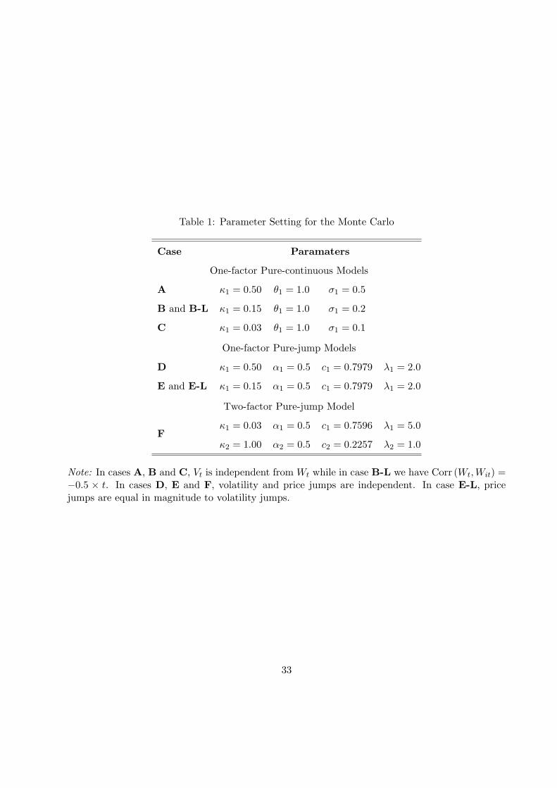
Table 1: Parameter Setting for the Monte Carlo

Case Paramaters

One-factor Pure-continuous Models

A κ1 = 0.50 θ1 = 1.0 σ1 = 0.5

B and B-L κ1 = 0.15 θ1 = 1.0 σ1 = 0.2

C κ1 = 0.03 θ1 = 1.0 σ1 = 0.1

One-factor Pure-jump Models

D κ1 = 0.50 α1 = 0.5 c1 = 0.7979 λ1 = 2.0

E and E-L κ1 = 0.15 α1 = 0.5 c1 = 0.7979 λ1 = 2.0

Two-factor Pure-jump Model

Fκ1 = 0.03 α1 = 0.5 c1 = 0.7596 λ1 = 5.0

κ2 = 1.00 α2 = 0.5 c2 = 0.2257 λ2 = 1.0

Note: In cases A, B and C, Vt is independent from Wt while in case B-L we have Corr (Wt,Wit) =−0.5 × t. In cases D, E and F, volatility and price jumps are independent. In case E-L, pricejumps are equal in magnitude to volatility jumps.

33

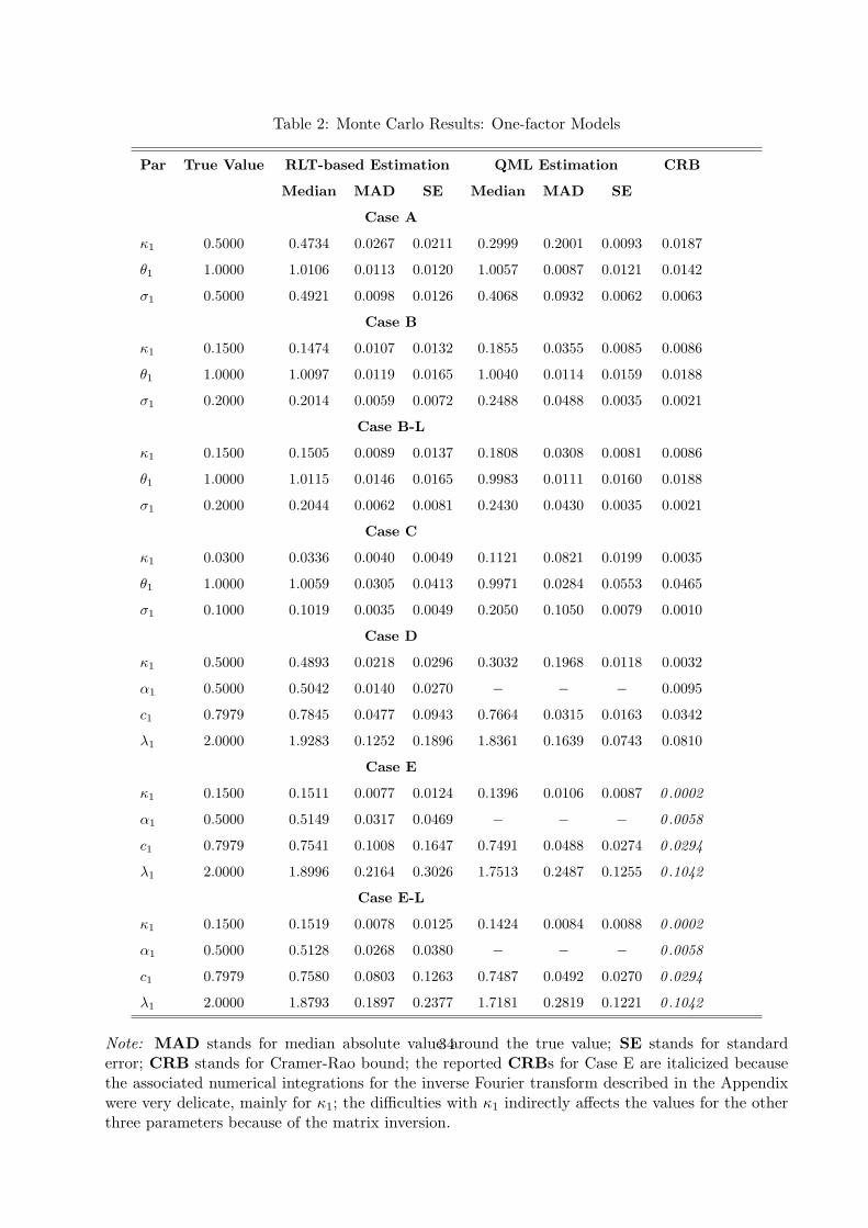
Table 2: Monte Carlo Results: One-factor Models

Par True Value RLT-based Estimation QML Estimation CRB

Median MAD SE Median MAD SE

Case A

κ1 0.5000 0.4734 0.0267 0.0211 0.2999 0.2001 0.0093 0.0187

θ1 1.0000 1.0106 0.0113 0.0120 1.0057 0.0087 0.0121 0.0142

σ1 0.5000 0.4921 0.0098 0.0126 0.4068 0.0932 0.0062 0.0063

Case B

κ1 0.1500 0.1474 0.0107 0.0132 0.1855 0.0355 0.0085 0.0086

θ1 1.0000 1.0097 0.0119 0.0165 1.0040 0.0114 0.0159 0.0188

σ1 0.2000 0.2014 0.0059 0.0072 0.2488 0.0488 0.0035 0.0021

Case B-L

κ1 0.1500 0.1505 0.0089 0.0137 0.1808 0.0308 0.0081 0.0086

θ1 1.0000 1.0115 0.0146 0.0165 0.9983 0.0111 0.0160 0.0188

σ1 0.2000 0.2044 0.0062 0.0081 0.2430 0.0430 0.0035 0.0021

Case C

κ1 0.0300 0.0336 0.0040 0.0049 0.1121 0.0821 0.0199 0.0035

θ1 1.0000 1.0059 0.0305 0.0413 0.9971 0.0284 0.0553 0.0465

σ1 0.1000 0.1019 0.0035 0.0049 0.2050 0.1050 0.0079 0.0010

Case D

κ1 0.5000 0.4893 0.0218 0.0296 0.3032 0.1968 0.0118 0.0032

α1 0.5000 0.5042 0.0140 0.0270 − − − 0.0095

c1 0.7979 0.7845 0.0477 0.0943 0.7664 0.0315 0.0163 0.0342

λ1 2.0000 1.9283 0.1252 0.1896 1.8361 0.1639 0.0743 0.0810

Case E

κ1 0.1500 0.1511 0.0077 0.0124 0.1396 0.0106 0.0087 0 .0002

α1 0.5000 0.5149 0.0317 0.0469 − − − 0 .0058

c1 0.7979 0.7541 0.1008 0.1647 0.7491 0.0488 0.0274 0 .0294

λ1 2.0000 1.8996 0.2164 0.3026 1.7513 0.2487 0.1255 0 .1042

Case E-L

κ1 0.1500 0.1519 0.0078 0.0125 0.1424 0.0084 0.0088 0 .0002

α1 0.5000 0.5128 0.0268 0.0380 − − − 0 .0058

c1 0.7979 0.7580 0.0803 0.1263 0.7487 0.0492 0.0270 0 .0294

λ1 2.0000 1.8793 0.1897 0.2377 1.7181 0.2819 0.1221 0 .1042

Note: MAD stands for median absolute value around the true value; SE stands for standarderror; CRB stands for Cramer-Rao bound; the reported CRBs for Case E are italicized becausethe associated numerical integrations for the inverse Fourier transform described in the Appendixwere very delicate, mainly for κ1; the difficulties with κ1 indirectly affects the values for the otherthree parameters because of the matrix inversion.

34

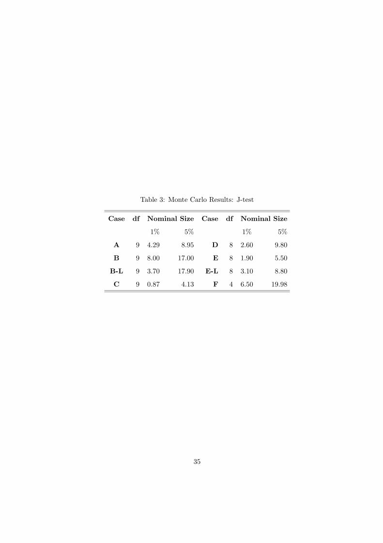
Table 3: Monte Carlo Results: J-test

Case df Nominal Size Case df Nominal Size

1% 5% 1% 5%

A 9 4.29 8.95 D 8 2.60 9.80

B 9 8.00 17.00 E 8 1.90 5.50

B-L 9 3.70 17.90 E-L 8 3.10 8.80

C 9 0.87 4.13 F 4 6.50 19.98

35

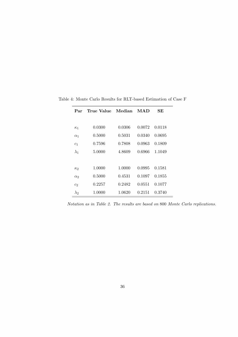
Table 4: Monte Carlo Results for RLT-based Estimation of Case F

Par True Value Median MAD SE

κ1 0.0300 0.0306 0.0072 0.0118

α1 0.5000 0.5031 0.0340 0.0695

c1 0.7596 0.7808 0.0963 0.1809

λ1 5.0000 4.8609 0.6966 1.1049

κ2 1.0000 1.0000 0.0995 0.1581

α2 0.5000 0.4531 0.1097 0.1855

c2 0.2257 0.2482 0.0551 0.1077

λ2 1.0000 1.0620 0.2151 0.3740

Notation as in Table 2. The results are based on 800 Monte Carlo replications.

36

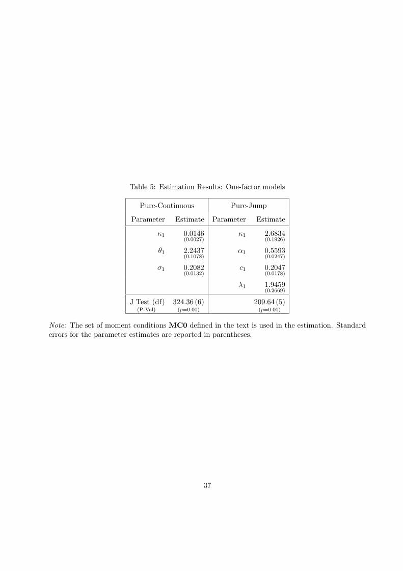
Table 5: Estimation Results: One-factor models

Pure-Continuous Pure-Jump

Parameter Estimate Parameter Estimate

κ1 0.0146(0.0027)

κ1 2.6834(0.1926)

θ1 2.2437(0.1078)

α1 0.5593(0.0247)

σ1 0.2082(0.0132)

c1 0.2047(0.0178)

λ1 1.9459(0.2669)

J Test (df)(P-Val)

324.36 (6)(p=0.00)

209.64 (5)(p=0.00)

Note: The set of moment conditions MC0 defined in the text is used in the estimation. Standarderrors for the parameter estimates are reported in parentheses.

37

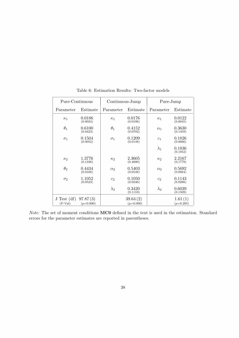
Table 6: Estimation Results: Two-factor models

Pure-Continuous Continuous-Jump Pure-Jump

Parameter Estimate Parameter Estimate Parameter Estimate

κ1 0.0186(0.0024)

κ1 0.0176(0.0106)

κ1 0.0122(0.0045)

θ1 0.6100(0.0423)

θ1 0.4152(0.0702)

α1 0.3630(0.1459)

σ1 0.1504(0.0052)

σ1 0.1209(0.0148)

c1 0.1826(0.0666)

λ1 0.1836(0.1852)

κ2 1.3776(0.1336)

κ2 2.3605(0.4000)

κ2 2.2167(0.1779)

θ2 0.4434(0.0168)

α2 0.5403(0.0548)

α2 0.5692(0.0864)

σ2 1.1052(0.0523)

c2 0.1050(0.0246)

c2 0.1143(0.0286)

λ2 0.3420(0.1110)

λ2 0.6039(0.1509)

J Test (df)(P-Val)

97.87 (3)(p=0.000)

39.64 (2)(p=0.000)

1.61 (1)(p=0.205)

Note: The set of moment conditions MC0 defined in the text is used in the estimation. Standarderrors for the parameter estimates are reported in parentheses.

38

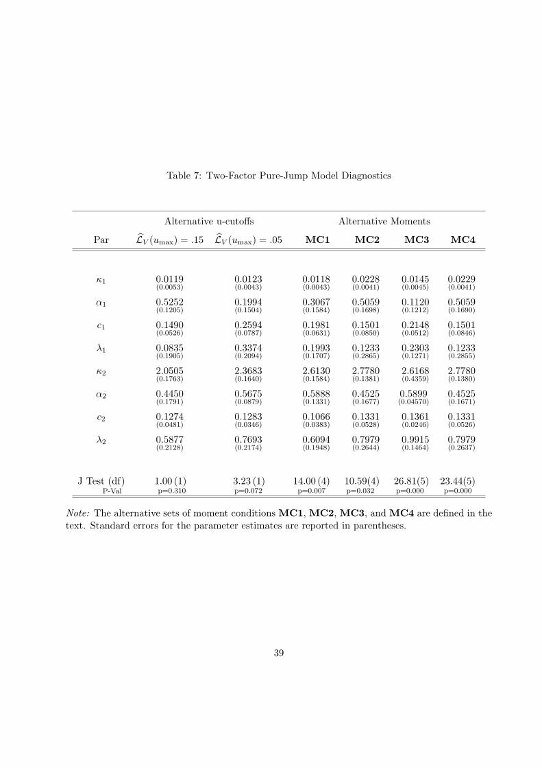
Table 7: Two-Factor Pure-Jump Model Diagnostics

Alternative u-cutoffs Alternative Moments

Par LV (umax) = .15 LV (umax) = .05 MC1 MC2 MC3 MC4

κ1 0.0119(0.0053)

0.0123(0.0043)

0.0118(0.0043)

0.0228(0.0041)

0.0145(0.0045)

0.0229(0.0041)

α1 0.5252(0.1205)

0.1994(0.1504)

0.3067(0.1584)

0.5059(0.1698)

0.1120(0.1212)

0.5059(0.1690)

c1 0.1490(0.0526)

0.2594(0.0787)

0.1981(0.0631)

0.1501(0.0850)

0.2148(0.0512)

0.1501(0.0846)

λ1 0.0835(0.1905)

0.3374(0.2094)

0.1993(0.1707)

0.1233(0.2865)

0.2303(0.1271)

0.1233(0.2855)

κ2 2.0505(0.1763)

2.3683(0.1640)

2.6130(0.1584)

2.7780(0.1381)

2.6168(0.4359)

2.7780(0.1380)

α2 0.4450(0.1791)

0.5675(0.0879)

0.5888(0.1331)

0.4525(0.1677)

0.5899(0.04570)

0.4525(0.1671)

c2 0.1274(0.0481)

0.1283(0.0346)

0.1066(0.0383)

0.1331(0.0528)

0.1361(0.0246)

0.1331(0.0526)

λ2 0.5877(0.2128)

0.7693(0.2174)

0.6094(0.1948)

0.7979(0.2644)

0.9915(0.1464)

0.7979(0.2637)

J Test (df)P-Val

1.00 (1)p=0.310

3.23 (1)p=0.072

14.00 (4)p=0.007

10.59(4)p=0.032

26.81(5)p=0.000

23.44(5)p=0.000

Note: The alternative sets of moment conditions MC1, MC2, MC3, and MC4 are defined in thetext. Standard errors for the parameter estimates are reported in parentheses.

39

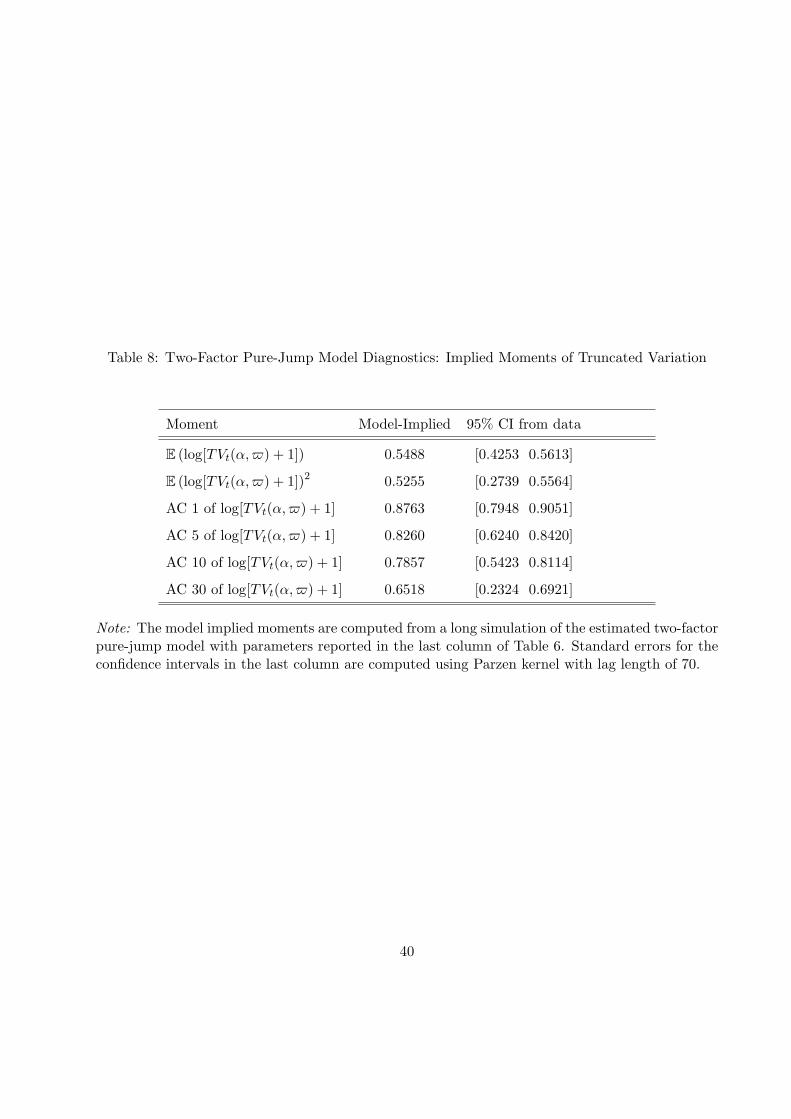
Table 8: Two-Factor Pure-Jump Model Diagnostics: Implied Moments of Truncated Variation

Moment Model-Implied 95% CI from data

E (log[TVt(α,ϖ) + 1]) 0.5488 [0.4253 0.5613]

E (log[TVt(α,ϖ) + 1])2 0.5255 [0.2739 0.5564]

AC 1 of log[TVt(α,ϖ) + 1] 0.8763 [0.7948 0.9051]

AC 5 of log[TVt(α,ϖ) + 1] 0.8260 [0.6240 0.8420]

AC 10 of log[TVt(α,ϖ) + 1] 0.7857 [0.5423 0.8114]

AC 30 of log[TVt(α,ϖ) + 1] 0.6518 [0.2324 0.6921]

Note: The model implied moments are computed from a long simulation of the estimated two-factorpure-jump model with parameters reported in the last column of Table 6. Standard errors for theconfidence intervals in the last column are computed using Parzen kernel with lag length of 70.

40

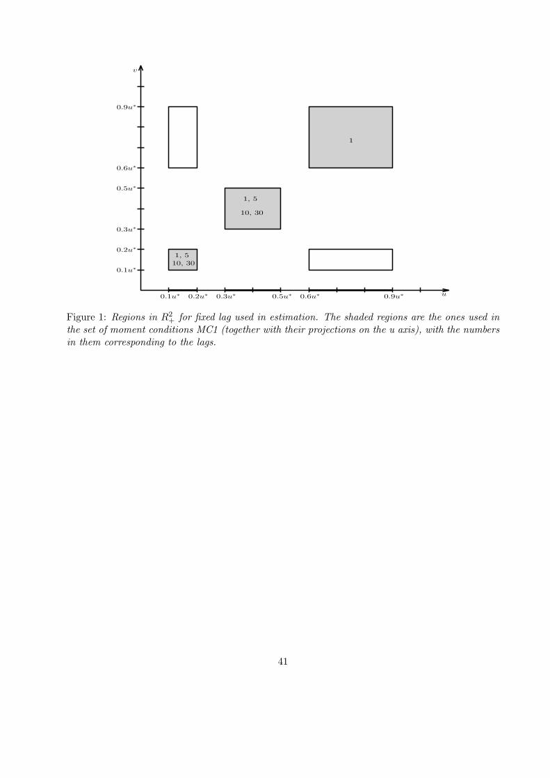
0.1u∗ 0.2u∗ 0.3u∗ 0.6u∗0.5u∗ 0.9u∗ u

0.1u∗

0.2u∗

0.3u∗

0.5u∗

0.6u∗

0.9u∗

v

1, 5

10, 30

1

1, 5

10, 30

Figure 1: Regions in R2+ for fixed lag used in estimation. The shaded regions are the ones used in

the set of moment conditions MC1 (together with their projections on the u axis), with the numbersin them corresponding to the lags.

41

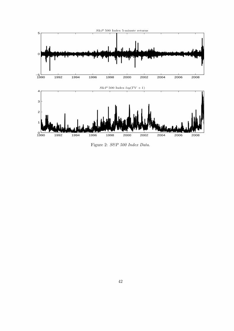
1990 1992 1994 1996 1998 2000 2002 2004 2006 2008−5

0

5S&P 500 Index 5-minute returns

1990 1992 1994 1996 1998 2000 2002 2004 2006 20080

1

2

3

4S&P 500 Index log(TV + 1)

Figure 2: S&P 500 Index Data.

42

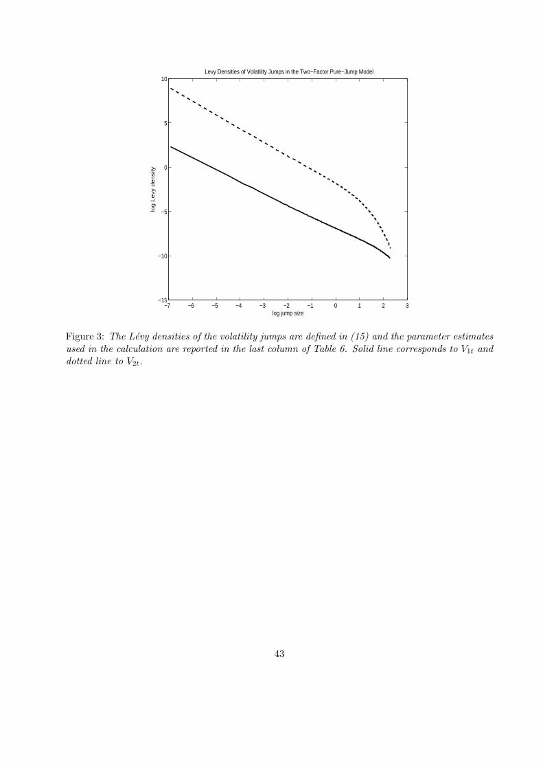
−7 −6 −5 −4 −3 −2 −1 0 1 2 3−15

−10

−5

0

5

10

log jump size

log

Le

vy d

en

sity

Levy Densities of Volatility Jumps in the Two−Factor Pure−Jump Model

Figure 3: The Levy densities of the volatility jumps are defined in (15) and the parameter estimatesused in the calculation are reported in the last column of Table 6. Solid line corresponds to V1t anddotted line to V2t.

43

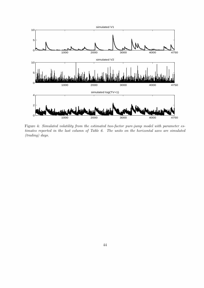
1000 2000 3000 4000 47500

5

10simulated V1

1000 2000 3000 4000 47500

5

10simulated V2

1000 2000 3000 4000 47500

2

4simulated log(TV+1)

Figure 4: Simulated volatility from the estimated two-factor pure-jump model with parameter es-timates reported in the last column of Table 6. The units on the horizontal axes are simulated(trading) days.

44