Real-World Repetition Estimation by Div, Grad and Curl

Tom F. H. Runia Cees G. M. Snoek Arnold W. M. Smeulders

QUVA Deep Vision Lab, University of Amsterdam

{runia,cgmsnoek,a.w.m.smeulders}@uva.nl

Abstract

We consider the problem of estimating repetition in video,

such as performing push-ups, cutting a melon or playing

violin. Existing work shows good results under the as-

sumption of static and stationary periodicity. As realistic

video is rarely perfectly static and stationary, the often pre-

ferred Fourier-based measurements is inapt. Instead, we

adopt the wavelet transform to better handle non-static and

non-stationary video dynamics. From the flow field and its

differentials, we derive three fundamental motion types and

three motion continuities of intrinsic periodicity in 3D. On

top of this, the 2D perception of 3D periodicity considers

two extreme viewpoints. What follows are 18 fundamental

cases of recurrent perception in 2D. In practice, to deal

with the variety of repetitive appearance, our theory implies

measuring time-varying flow Ft and its differentials ∇Ft ,

∇ · Ft and ∇ × Ft over segmented foreground motion. For

experiments, we introduce the new QUVA Repetition dataset,

reflecting reality by including non-static and non-stationary

videos. On the task of counting repetitions in video, we obtain

favorable results compared to a deep learning alternative.

1. Introduction

Visual repetition is ubiquitous in the world around us. It is

present in activities like rowing, music-making and cooking.

It arises in natural and urban environments: traffic patterns,

blinking lights, and leaves in the wind. Rhythm and repeti-

tion are used to approximate velocity, estimate progress and

to trigger attention [13]. In computer vision, understanding

repetition in video is important as it can serve action classi-

fication [9, 17], action localization [14, 24], human motion

analysis [1, 21], 3D reconstruction [3] and camera calibration

[12]. Estimating repetition remains challenging. First and

foremost, repetition appears in many forms due to its variety

in motion pattern and motion continuity. The viewpoint is

crucial for the perception of recurrence. In practice, camera

motion makes repetition estimation inevitably hard.

Existing work on repetition estimation in video [15, 19]

reports good results under the assumption that the motion is

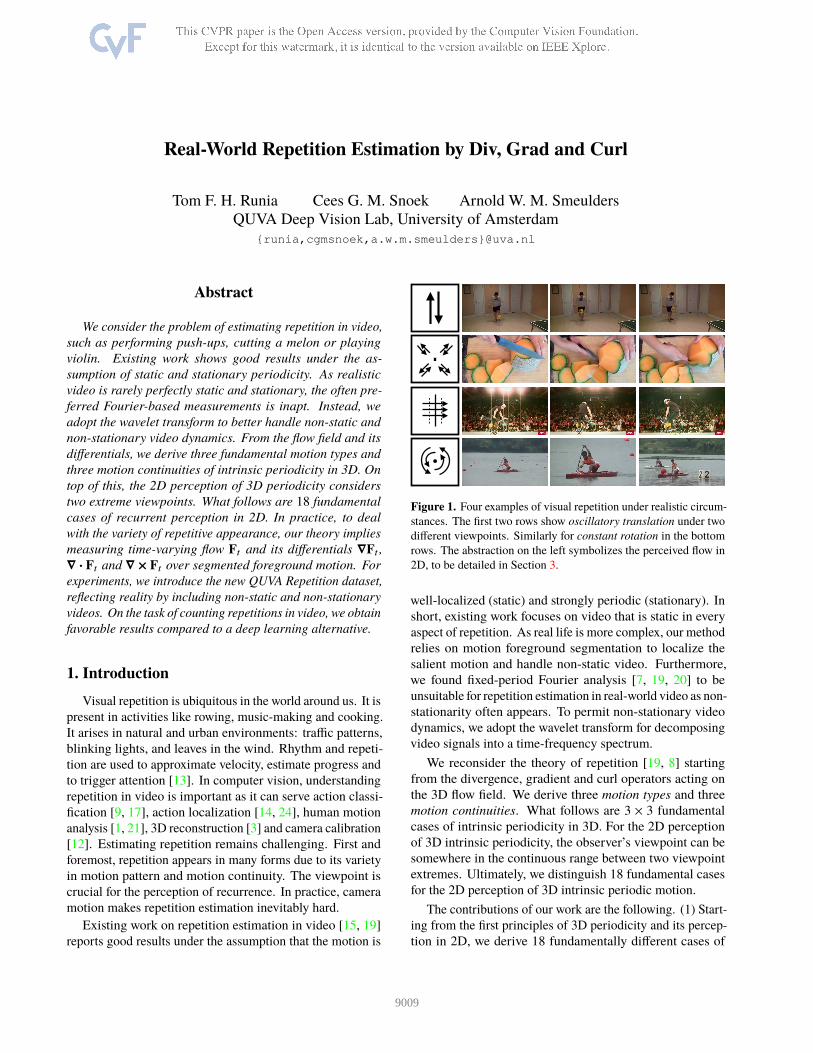
Figure 1. Four examples of visual repetition under realistic circum-

stances. The first two rows show oscillatory translation under two

different viewpoints. Similarly for constant rotation in the bottom

rows. The abstraction on the left symbolizes the perceived flow in

2D, to be detailed in Section 3.

well-localized (static) and strongly periodic (stationary). In

short, existing work focuses on video that is static in every

aspect of repetition. As real life is more complex, our method

relies on motion foreground segmentation to localize the

salient motion and handle non-static video. Furthermore,

we found fixed-period Fourier analysis [7, 19, 20] to be

unsuitable for repetition estimation in real-world video as non-

stationarity often appears. To permit non-stationary video

dynamics, we adopt the wavelet transform for decomposing

video signals into a time-frequency spectrum.

We reconsider the theory of repetition [19, 8] starting

from the divergence, gradient and curl operators acting on

the 3D flow field. We derive three motion types and three

motion continuities. What follows are 3 × 3 fundamental

cases of intrinsic periodicity in 3D. For the 2D perception

of 3D intrinsic periodicity, the observer’s viewpoint can be

somewhere in the continuous range between two viewpoint

extremes. Ultimately, we distinguish 18 fundamental cases

for the 2D perception of 3D intrinsic periodic motion.

The contributions of our work are the following. (1) Start-

ing from the first principles of 3D periodicity and its percep-

tion in 2D, we derive 18 fundamentally different cases of

9009

repetitive perception. (2) To estimate repetition in video un-

der realistic circumstances, we compute a diverse flow-based

representation over the motion foreground segmentation. Our

method uses wavelets to handle non-stationary motion and

automatically selects the most discriminative signal based

on self-estimated quality assessment. (3) Extending beyond

the video dataset of [15], we propose the new QUVA Repeti-

tion dataset for repetition estimation, that is more realistic

and challenging by lifting the static and stationary assump-

tions. (4) We evaluate on the task of repetition counting and

show that our method outperforms the deep learning-based

state-of-the-art [15] on the new dataset.

2. Related Work

Existing approaches for repetition estimation in video

typically represent video as one-dimensional signals that pre-

serve the repetitive structure of the motion. Then, frequency

information is extracted by Fourier analysis [2, 7, 19, 30],

peak detection [28] or singular value decomposition [6].

Pogalin et al. [19] estimate the frequency of motion in video

by tracking an object, performing principal component analy-

sis over the tracked regions and employing the Fourier-based

periodogram. However, methods relying on Fourier-analysis

for periodic motion are unable, nor intended, to handle

non-stationary motion as is ubiquitous in the real world.

Briassouli & Ahuja [4] employ time-frequency analysis

using the Short Time Fourier Transform for dealing with

multiple periodic motions. In [5], the authors propose a

spatiotemporal filter bank for estimating repetition in video.

Their filters work online and are effective when tuned cor-

rectly. However, we question its practical use, as their

experiment are limited to stationary motion and the filter

bank requires manual tuning. We also use a time-frequency

decomposition of signals from video, but concentrate on

handling non-stationary repetition. Instead of using the

Short-Time Fourier Transform, we adopt the continuous

wavelet transform to achieve better resolution [23].

The studies on periodic motion by [8, 19, 26] have en-

couraged us to reconsider visual repetition. Pogalin et al.

[19] identify four visually periodic motion types (translation,

rotation, deformation and intensity variation) supplemented

with three cases of motion continuity (oscillating, constant

and intermittent) in the 2D field of view. In this work, we

argue that the 3D flow field is the right starting point to

derive the foundations of repetition. From the 3D flow field

and the differential operators acting on it, we derive three

motion types and three motion continuities that organize

into a 3 × 3 Cartesian table. Moreover, the projection of 3D

periodicity on 2D perception has to consider the viewpoint.

What follows are 18 fundamentally different cases of 2D

repetitive perception from 3D periodicity.

Levy & Wolf [15] introduce a convolutional neural net-

work for estimating repetition by counting in live video. Their

network is trained to predict the motion period on synthetic

video sequences in which moving squares exhibit periodic

motion of four motion types from [19]. At test time, the

method takes a stack of video frames, computes a region

of interest by motion thresholding, and forwards the frame

crops through the network to classify the motion period. The

system is evaluated on the task of repetition counting and

shows near-perfect performance on their YTSegments dataset.

The 100 videos are a good initial set of examples but as

the majority of videos have static viewpoint and exhibit sta-

tionary periodic repetitions, we propose a new dataset. Our

dataset better reflects reality by including more non-static

and non-stationary examples. Similar to Levy & Wolf, we

also evaluate repetition estimation by counting.

3. Theory

3.1. 3D Intrinsic Periodicity

In 3D, intrinsic periodicity is defined as the reappearing

of the same 3D-flow F (x, t) induced by the motion of an

object over time. For a moment in time t, we denote the flow

by Ft (x). The 3D-flow field tied to the object is periodic as

expressed by Ft (x) = Ft+T (x+S), where we exclude for the

moment the trivial case that the flow field is constant. The

parameter T is the period over time, where S is the period, if

any, over space.

Let the flow field be given by its directional components:

Ft = (Fx, Fy, Fz ). From differential geometry, we have the

three operators on the flow field:

∇Ft =∂Fk

∂x j

ej ⊗ ek (1)

∇ ·Ft =∂Fx

∂x+

∂Fy

∂y+

∂Fz

∂z(2)

∇ ×Ft =

(

∂Fz

∂y−∂Fy

∂z,∂Fx

∂z−∂Fz

∂x,∂Fy

∂x−∂Fx

∂y

)

. (3)

Where in Eq. (1) the product ej ⊗ ek defines a dyadic tensor,

and indices are summed over the 9 terms by the Einstein con-

vention [27]. The equations define the gradient, divergence

and curl of the flow field [25]. Three basic 3D-motion types

emerge depending on the values of divergence and curl as

follows:

translation: ∇ ×Ft = 0, ∇ ·Ft = 0

rotation: ∇ ×Ft , 0, ∇ ·Ft = 0

expansion: ∇ ×Ft = 0, ∇ ·Ft , 0.

In practice there may be a mixture types; as we are aiming to

handle realistic video, we select the dominant 3D-periodicity

in the object’s motion whichever is measurable best. In the

rare case of counterbalancing expansion and contraction over

different axes, it can be that ∇ ·Ft = 0 while being periodic.

9010

constant intermittent oscillatory

translation

rotation

exp

ansion

(a) Flow Abstractions in 3D

constant intermittent oscillatory

translation

rotation

exp

ansion

(b) Examples in Real Life

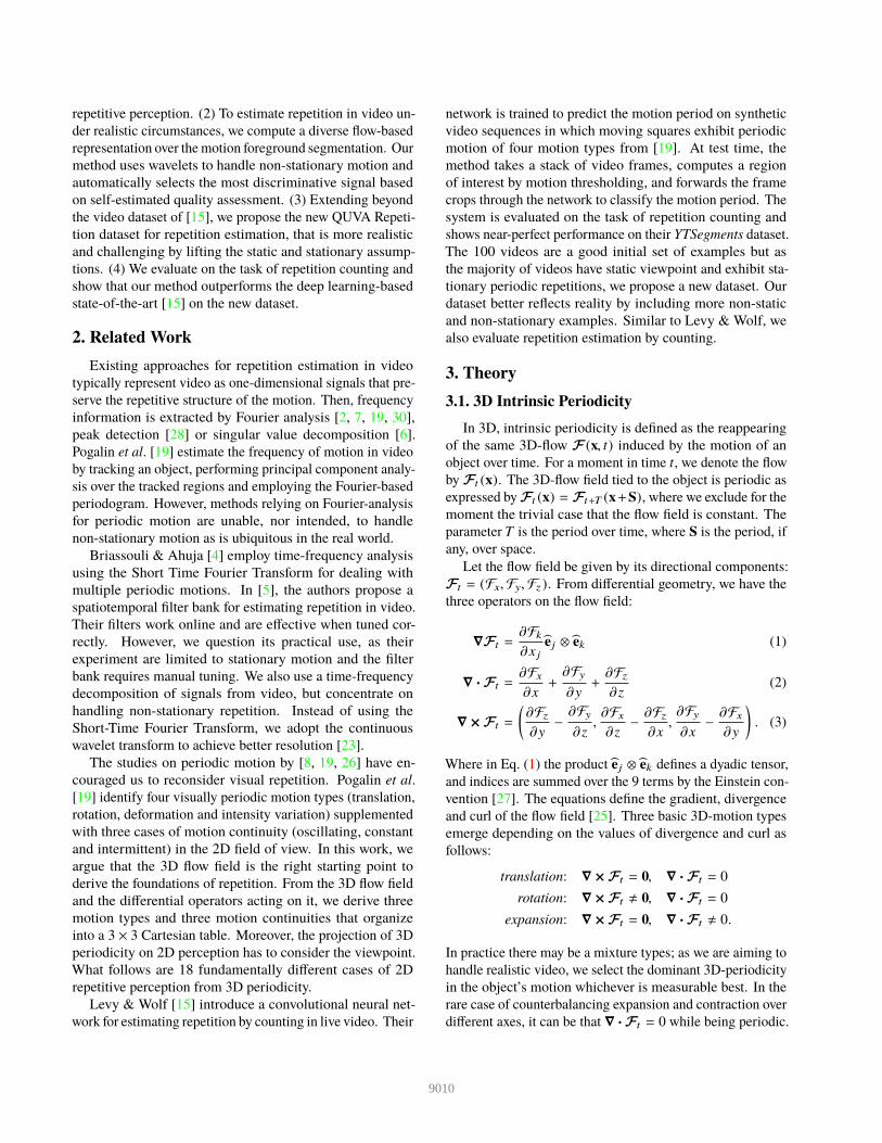
Figure 2. 3 × 3 Cartesian table of the motion type times the motion continuity. Following from the differential operators acting on the flow,

these are the basic cases of periodicity in 3D. The examples are: escalator, leaping frog, bouncing ball, pirouette, tightening a bolt, laundry

machine, inflating a tire, inflating a balloon and a breathing anemone.

In addition, the motion continuity in 3D can be a source

of periodicity. Depending on the type of motion, the motion

field needs fulfill one of the following necessary periodic

conditions:

∇Ft (x) = ∇Ft+T (x + ǫ )

∇ ×Ft (x) = ∇ ×Ft+T (x + ǫ )

∇ ·Ft (x) = ∇ ·Ft+T (x + ǫ ),

where ǫ denotes a translation as the object’s periodicity may

be superposed on translation. For robustness to illumina-

tion changes, the measurement of ∇Ft (x) is preferred over

Ft . From these equations three different periodic motion

continuities can be distinguished: constant, intermittent

and oscillating periodicity. Again, in practice the motion

continuity may be a mixture between types.

3.2. 2D Recurrence of 3D Intrinsic Periodicity

So far we have considered the intrinsic periodicity in 3D.

We reserve the term recurrent for the 2D observation of the

3D periodicity. Recurrence in the field of view is defined by:

Ft (x) = Ft+T (σ(x + s)), (4)

where Ft (x) is perceived flow in 2D image coordinates x, s is

the observed displacement, T is the recurrence and σ denotes

the observational scale (camera zoom). The underlying

principle is that the same period length T will be observed in

both 3D and 2D for all cases of intrinsic periodicity. As we

perform all measurements within one image, from here on

F(x) implies Ft (x) where subscript t is omitted for clarity.

In addition, the intrinsic periodicity in 3D does not cover

all perceived recurrence in an image sequence. For the trivial

cases of constant translation and constant expansion in 3D,

perceived recurrence will appear when a repetitive chain of

objects (conveyor belt) or a repetitive appearance (checkered

balloon) on the object, as given by Equation 4, is aligned with

the motion. In such cases, recurrence will also be observed

in the field of view. For constant rotation, the restriction is

that the appearance cannot be constant over the surface, as

no motion, let alone recurrent motion would be observed. In

the rotational case, any rotational symmetry in appearance

will induce a higher order recurrence as a multiplication of

the symmetry and the rotational speed.

For the purpose of recurrence, nine cases organize in

a 3 × 3 Cartesian table of basic motion type times motion

continuity, see Figure 2a. The corresponding examples of

these nine cases are given in Figure 2b. This is the list of

fundamental cases, where a mixture of types is permitted.

In practice, some cases are ubiquitous, while for others it is

hard to find examples at all and a mixture of types is rare.

3.3. The Viewpoint

The point of view has a large influence on the perception

of the flow field. There are two fundamentally different

viewpoints: the frontal view and the side view:

frontal view: on the main axis of motion

side view: perpendicular to the main axis of motion.

For translation there is one main axis and two perpendicu-

lar axes, which are both identical for our purpose. There is no

9011

translation

rotation

expansion

constant intermittent back-and-forth

Side View Front View

1 2

4 5

10

13

167 8

11

14

17

3

6

9

12

15

18

constant intermittent back-and-forth

translation

rotation

expansion

constant intermittent oscillating

Side View Front View

1 2

7 8

4

10

1613 14

5

11

17

3

9

15

6

12

18

constant intermittent oscillating

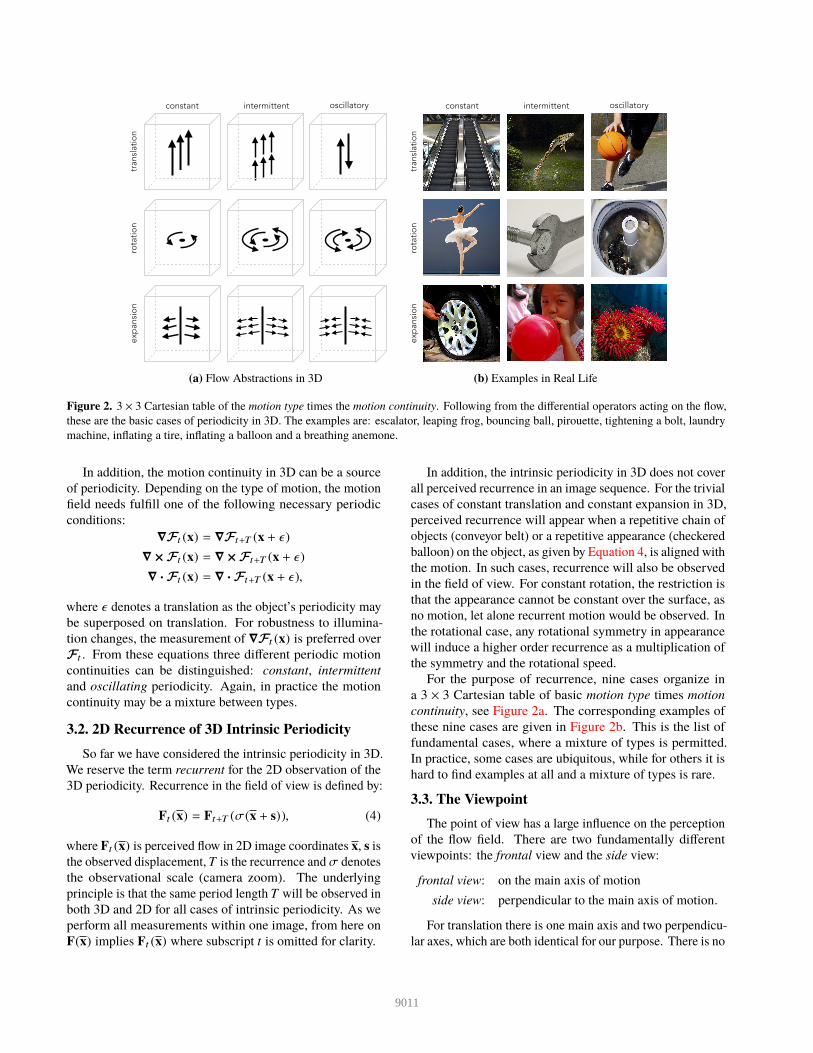
Figure 3. Observed flow: the 18 fundamental cases for 2D perception of 3D recurrence. The perception follows from the motion pattern

(3×), motion continuity (3×) and the viewpoint on the continuous interval between the two extremes: side and front view. ↑ denotes flow

direction, � denotes a vanishing point, • denotes a rotation point, ⋆ denotes expansion point. Dashed grey lines for constant motion indicate

the need for texture to perceive recurrence. Pairs 4-16, 5-17 and 6-18 appear similar at first sight but vary in their signal profile.

distinction between the two perpendicular views. Similarly,

for rotation the two perpendicular cases are also indistin-

guishable. For expansion there are one, two or three axes

of expansion, again leaving us with the frontal case and

the perpendicular case as the two fundamental cases. Con-

sequently, for all cases considered, a distinction between

frontal view and side view is sufficient. As a result, the per-

ceived recurrence is summarized between the two extreme

viewpoints, which results in the Cartesian product of two

times nine basic cases as summarized in Figure 3. The two

views are the end of a continuous range of viewpoints. An

actual viewpoint will be somewhere in between the frontal

view and the side view, most of the time. This leaves the

flow field asymmetrical or skewed, either in gradient, curl or

divergence. As long as the signal can be measured this will

not affect the recurrent nature of the signal.

3.4. Non-Static Repetition

So far we have assumed a static camera position. In

particular with recurrent motion (1) the camera may move

itself because the camera is mounted on the moving object

itself, or (2) the camera is following the target of interest,

or (3) the camera is in motion independent of the motion

of the object. For the first two cases, the camera motion

reflects the periodic dynamics of the object’s motion. The

flow field may be outside the object, but otherwise it displays

a complementary pattern in the flow field.

Only the third case demands removal of the camera mo-

tion prior to the repetitive motion analysis. In practice, this

situation occurs frequently. Therefore, particular attention

needs to be paid to camera motion independent of the target’s

motion. When due to the camera motion, the viewpoint

changes from frontal to side view, the analysis will be in-

evitably hard. Figure 3 illustrates the dramatic changes in

the flow field when the camera changes from one extreme

viewpoint (side) to the other (frontal), or vice versa.

In addition, even when object motion and camera are both

static, for none of the intrinsic motion types (translation,

rotation, expansion), a point on the object will be at the

same position in the camera field all the time. Under the

double static condition, a point will just return to the same

point on the camera field. As the intermediate points on the

object or background have an arbitrary albedo and radiate

an arbitrary luminance, no sinusoidal signal will result in

general. This is noteworthy as all previous work [7, 16, 19]

implicitly assumed such a signal by considering the Fourier

transform or variants.

3.5. Non-Stationary Repetition

A recurrent signal is said to be stationary when the pe-

riod length is constant over time. In the initial steps of

periodicity analysis, it was assumed the periodic signal was

near-stationary. In practice, we have observed that stationary

repetitive signals are relatively rare. Decay in frequency or

accelerating motion are common in realistic video. There-

fore, in contrast to [7, 19] we do not assume stationarity,

making the method more robust to acceleration. We will

employ local wavelets in response to the anticipated signals.

4. Repetition Estimation

Our method for repetition estimation follows a three-

stage approach (Figure 4). First, we localize the target

instance in the scene, then we represent the target by a set of

time-varying signals and finally we perform time-frequency

9012

rxF

time

Am

plit

ud

eS

cale

(lo

g s

cale

)

ryF

Time Time Time Time

r · F r× F

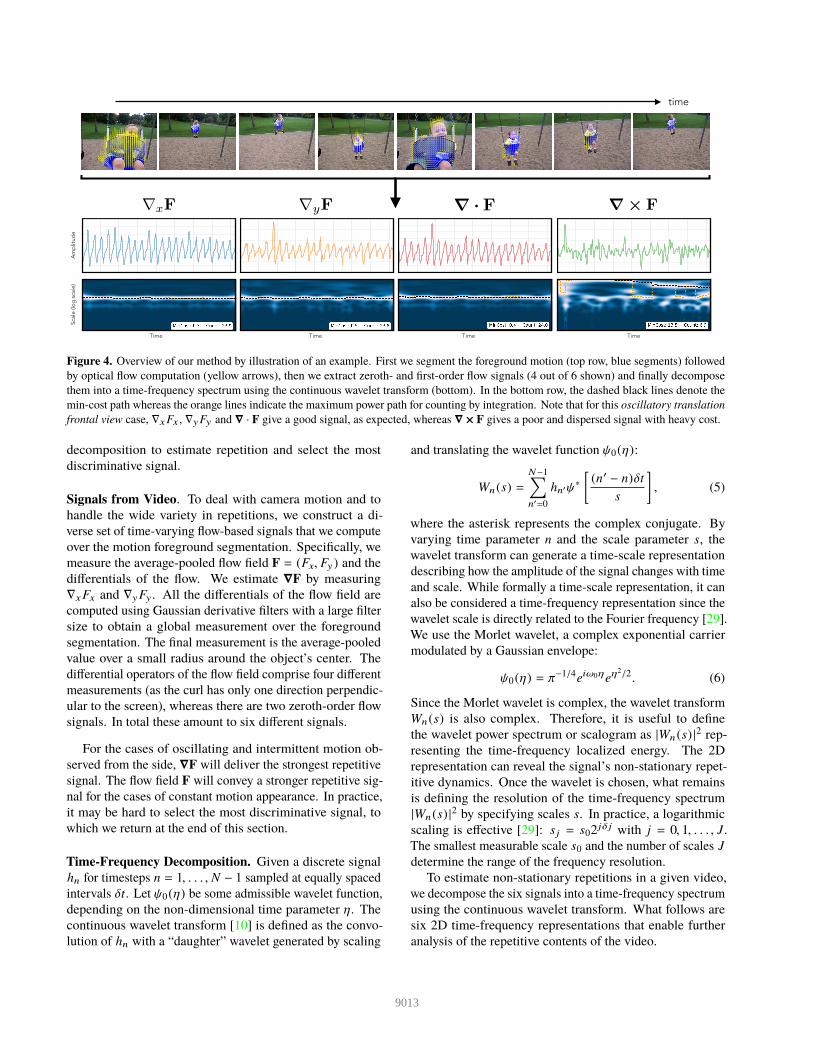
Figure 4. Overview of our method by illustration of an example. First we segment the foreground motion (top row, blue segments) followed

by optical flow computation (yellow arrows), then we extract zeroth- and first-order flow signals (4 out of 6 shown) and finally decompose

them into a time-frequency spectrum using the continuous wavelet transform (bottom). In the bottom row, the dashed black lines denote the

min-cost path whereas the orange lines indicate the maximum power path for counting by integration. Note that for this oscillatory translation

frontal view case, ∇xFx , ∇yFy and ∇ · F give a good signal, as expected, whereas ∇ × F gives a poor and dispersed signal with heavy cost.

decomposition to estimate repetition and select the most

discriminative signal.

Signals from Video. To deal with camera motion and to

handle the wide variety in repetitions, we construct a di-

verse set of time-varying flow-based signals that we compute

over the motion foreground segmentation. Specifically, we

measure the average-pooled flow field F = (Fx, Fy ) and the

differentials of the flow. We estimate ∇F by measuring

∇xFx and ∇yFy . All the differentials of the flow field are

computed using Gaussian derivative filters with a large filter

size to obtain a global measurement over the foreground

segmentation. The final measurement is the average-pooled

value over a small radius around the object’s center. The

differential operators of the flow field comprise four different

measurements (as the curl has only one direction perpendic-

ular to the screen), whereas there are two zeroth-order flow

signals. In total these amount to six different signals.

For the cases of oscillating and intermittent motion ob-

served from the side, ∇F will deliver the strongest repetitive

signal. The flow field F will convey a stronger repetitive sig-

nal for the cases of constant motion appearance. In practice,

it may be hard to select the most discriminative signal, to

which we return at the end of this section.

Time-Frequency Decomposition. Given a discrete signal

hn for timesteps n = 1, . . . , N − 1 sampled at equally spaced

intervals δt. Let ψ0(η) be some admissible wavelet function,

depending on the non-dimensional time parameter η. The

continuous wavelet transform [10] is defined as the convo-

lution of hn with a “daughter” wavelet generated by scaling

and translating the wavelet function ψ0(η):

Wn(s) =

N−1∑

n′=0

hn′ψ∗

[(n′ − n)δt

s

], (5)

where the asterisk represents the complex conjugate. By

varying time parameter n and the scale parameter s, the

wavelet transform can generate a time-scale representation

describing how the amplitude of the signal changes with time

and scale. While formally a time-scale representation, it can

also be considered a time-frequency representation since the

wavelet scale is directly related to the Fourier frequency [29].

We use the Morlet wavelet, a complex exponential carrier

modulated by a Gaussian envelope:

ψ0(η) = π−1/4eiω0ηeη2/2. (6)

Since the Morlet wavelet is complex, the wavelet transform

Wn(s) is also complex. Therefore, it is useful to define

the wavelet power spectrum or scalogram as |Wn(s) |2 rep-

resenting the time-frequency localized energy. The 2D

representation can reveal the signal’s non-stationary repet-

itive dynamics. Once the wavelet is chosen, what remains

is defining the resolution of the time-frequency spectrum

|Wn(s) |2 by specifying scales s. In practice, a logarithmic

scaling is effective [29]: s j = s02jδ j with j = 0, 1, . . . , J.

The smallest measurable scale s0 and the number of scales J

determine the range of the frequency resolution.

To estimate non-stationary repetitions in a given video,

we decompose the six signals into a time-frequency spectrum

using the continuous wavelet transform. What follows are

six 2D time-frequency representations that enable further

analysis of the repetitive contents of the video.

9013

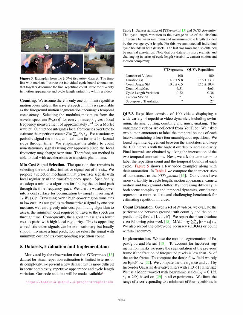
Figure 5. Examples from the QUVA Repetition dataset. The time-

line with markers illustrate the individual cycle bound annotations,

that together determine the final repetition count. Note the diversity

in motion appearance and cycle length variability within a video.

Counting. We assume there is only one dominant repetitive

motion observable in the wavelet spectrum; this is reasonable

as the foreground motion segmentation encourages temporal

consistency. Selecting the modulus maximum from the

wavelet spectrum |Wn(s) |2 for every timestep n gives a local

frequency measurement of approximately s−1 for a Morlet

wavelet. Our method integrates local frequencies over time to

estimate the repetition count: c =∑

n δt/sn. For a stationary

periodic signal the modulus maximum forms a horizontal

ridge through time. We emphasize the ability to count

non-stationary signals using our approach since the local

frequency may change over time. Therefore, our method is

able to deal with accelerations or transient phenomena.

Min-Cost Signal Selection. The question that remains is

selecting the most discriminative signal out of the six. We

propose a selection mechanism that prioritizes signals with

local regularity in the time-frequency space. Specifically,

we adopt a min-cost algorithm for finding the optimal path

through the time-frequency space. We turn the wavelet power

into a cost surface for optimization by simply inverting it:

1/|Wn(s) |2. Traversing over a high-power region translates

to low cost. As our goal is to characterize a signal by one cost

measure, we run a greedy min-cost pathfinding algorithm to

assess the minimum cost required to traverse the spectrum

through time. Consequently, the algorithm assigns a lower

cost to paths with high local regularity. This is appealing

as realistic video signals can be non-stationary but locally

smooth. To make a final prediction we select the signal with

minimum cost and its corresponding repetition count.

5. Datasets, Evaluation and Implementation

Motivated by the observation that the YTSegments [15]

dataset for visual repetition estimation is limited in terms of

its complexity, we present a new dataset that is more difficult

in scene complexity, repetitive appearance and cycle length

variation. Our code and data will be made available1.

1https://tomrunia.github.io/projects/repetition

Table 1. Dataset statistics of YTSegments [15] and QUVA Repetition.

The cycle length variation is the average value of the absolute

difference between minimum and maximum cycle length divided

by the average cycle length. For this, we annotated all individual

cycle bounds in both datasets. The last two rows are also obtained

by manual annotation. Note that our dataset is more realistic and

challenging in terms of cycle length variability, camera motion and

motion complexity.

YTSegments QUVA Repetition

Number of Videos 100 100

Duration (s) 14.9 ± 9.8 17.6 ± 13.3

Count Avg.± Std. 10.8 ± 6.5 12.5 ± 10.4

Count Min/Max 4/51 4/63

Cycle Length Variation 0.22 0.36

Camera Motion 21 53

Superposed Translation 7 27

QUVA Repetition consists of 100 videos displaying a

wide variety of repetitive video dynamics, including swim-

ming, stirring, cutting, combing and music-making. The

untrimmed videos are collected from YouTube. We asked

two human annotators to label the temporal bounds of each

interval containing at least four unambiguous repetitions. We

found high inter-agreement between the annotators and keep

the 100 intervals with the highest overlap to increase clarity.

Final intervals are obtained by taking the intersection of the

two temporal annotations. Next, we ask the annotators to

label the repetition count and the temporal bounds of each

cycle. Figure 5 shows a few video examples along with

their annotation. In Table 1 we compare the characteristics

of our dataset to the YTSegments [15]. Our videos have

more variability in cycle length, motion appearance, camera

motion and background clutter. By increasing difficulty in

both scene complexity and temporal dynamics, our dataset

represents a more realistic and challenging benchmark for

estimating repetition in video.

Count Evaluation. Given a set of N videos, we evaluate the

performance between ground truth count ci and the count

prediction ci for i ∈ {1, . . . , N }. We report the mean absolute

error following prior work [15]: MAE = 1N

∑Ni=1

��ci − ci �� /ci .We also record the off-by-one accuracy (OBOA) or count

within-1 accuracy.

Implementation. We use the motion segmentation of Pa-

pazoglou and Ferrari [18]. To account for incorrect seg-

mentation masks we reuse the segmentation of the previous

frame if the fraction of foreground pixels is less than 1% of

the entire frame. To compute the dense flow field we rely

on EpicFlow [22]. We compute the divergence and curl by

first-order Gaussian derivative filters with a 13×13 filter size.

We use a Morlet wavelet with logarithmic scales (δ j = 0.125,

s0 = 2δt) based on [29] in all experiments. We limit the

range of J corresponding to a minimum of four repetitions in

9014

0.0 0.2 0.4 0.6 0.8 1.0 1.2 1.4 1.6Cycle Length Variation

0

5

10

15

20

25

30

Rela

tive

Coun

t Err

or: |

c ic i

|/ci

Fourier and Wavelets for Counting Idealized Signals

Fourier. MAE = 7.3 ± 5.9, OBOA = 0.89Wavelets. MAE = 2.1 ± 1.7, OBOA = 0.99

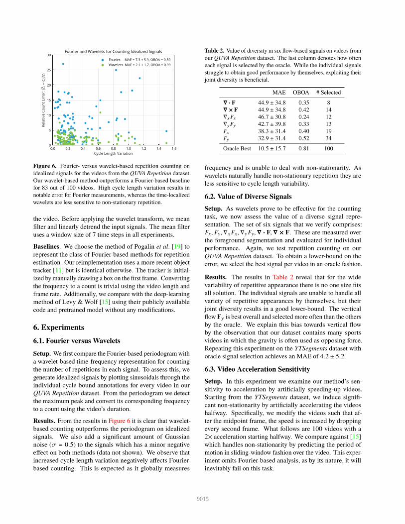
Figure 6. Fourier- versus wavelet-based repetition counting on

idealized signals for the videos from the QUVA Repetition dataset.

Our wavelet-based method outperforms a Fourier-based baseline

for 83 out of 100 videos. High cycle length variation results in

notable error for Fourier measurements, whereas the time-localized

wavelets are less sensitive to non-stationary repetition.

the video. Before applying the wavelet transform, we mean

filter and linearly detrend the input signals. The mean filter

uses a window size of 7 time steps in all experiments.

Baselines. We choose the method of Pogalin et al. [19] to

represent the class of Fourier-based methods for repetition

estimation. Our reimplementation uses a more recent object

tracker [11] but is identical otherwise. The tracker is initial-

ized by manually drawing a box on the first frame. Converting

the frequency to a count is trivial using the video length and

frame rate. Additionally, we compare with the deep-learning

method of Levy & Wolf [15] using their publicly available

code and pretrained model without any modifications.

6. Experiments

6.1. Fourier versus Wavelets

Setup. We first compare the Fourier-based periodogram with

a wavelet-based time-frequency representation for counting

the number of repetitions in each signal. To assess this, we

generate idealized signals by plotting sinusoidals through the

individual cycle bound annotations for every video in our

QUVA Repetition dataset. From the periodogram we detect

the maximum peak and convert its corresponding frequency

to a count using the video’s duration.

Results. From the results in Figure 6 it is clear that wavelet-

based counting outperforms the periodogram on idealized

signals. We also add a significant amount of Gaussian

noise (σ = 0.5) to the signals which has a minor negative

effect on both methods (data not shown). We observe that

increased cycle length variation negatively affects Fourier-

based counting. This is expected as it globally measures

Table 2. Value of diversity in six flow-based signals on videos from

our QUVA Repetition dataset. The last column denotes how often

each signal is selected by the oracle. While the individual signals

struggle to obtain good performance by themselves, exploiting their

joint diversity is beneficial.

MAE OBOA # Selected

∇ · F 44.9 ± 34.8 0.35 8

∇ × F 44.9 ± 34.8 0.42 14

∇xFx 46.7 ± 30.8 0.24 12

∇yFy 42.7 ± 39.8 0.33 13

Fx 38.3 ± 31.4 0.40 19

Fy 32.9 ± 31.4 0.52 34

Oracle Best 10.5 ± 15.7 0.81 100

frequency and is unable to deal with non-stationarity. As

wavelets naturally handle non-stationary repetition they are

less sensitive to cycle length variability.

6.2. Value of Diverse Signals

Setup. As wavelets prove to be effective for the counting

task, we now assess the value of a diverse signal repre-

sentation. The set of six signals that we verify comprises:

Fx, Fy,∇xFx,∇yFy,∇ · F,∇ × F. These are measured over

the foreground segmentation and evaluated for individual

performance. Again, we test repetition counting on our

QUVA Repetition dataset. To obtain a lower-bound on the

error, we select the best signal per video in an oracle fashion.

Results. The results in Table 2 reveal that for the wide

variability of repetitive appearance there is no one size fits

all solution. The individual signals are unable to handle all

variety of repetitive appearances by themselves, but their

joint diversity results in a good lower-bound. The vertical

flow Fy is best overall and selected more often than the others

by the oracle. We explain this bias towards vertical flow

by the observation that our dataset contains many sports

videos in which the gravity is often used as opposing force.

Repeating this experiment on the YTSegments dataset with

oracle signal selection achieves an MAE of 4.2 ± 5.2.

6.3. Video Acceleration Sensitivity

Setup. In this experiment we examine our method’s sen-

sitivity to acceleration by artificially speeding-up videos.

Starting from the YTSegments dataset, we induce signifi-

cant non-stationarity by artificially accelerating the videos

halfway. Specifically, we modify the videos such that af-

ter the midpoint frame, the speed is increased by dropping

every second frame. What follows are 100 videos with a

2× acceleration starting halfway. We compare against [15]

which handles non-stationarity by predicting the period of

motion in sliding-window fashion over the video. This exper-

iment omits Fourier-based analysis, as by its nature, it will

inevitably fail on this task.

9015

Levy & Wolf This Paper0

5

10

15

20

25

Mea

n Ab

solu

te E

rror

Sensitivity to Non-Stationarity by Halfway Acceleration

Original Speed2x Acceleration

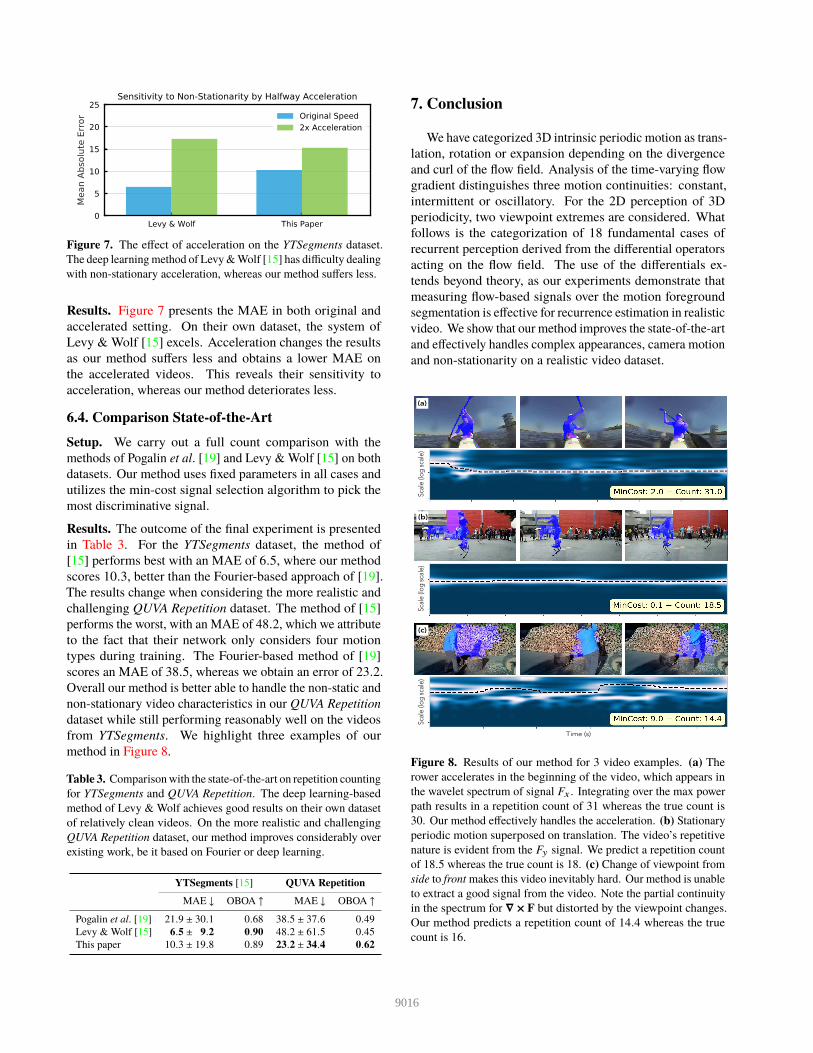
Figure 7. The effect of acceleration on the YTSegments dataset.

The deep learning method of Levy & Wolf [15] has difficulty dealing

with non-stationary acceleration, whereas our method suffers less.

Results. Figure 7 presents the MAE in both original and

accelerated setting. On their own dataset, the system of

Levy & Wolf [15] excels. Acceleration changes the results

as our method suffers less and obtains a lower MAE on

the accelerated videos. This reveals their sensitivity to

acceleration, whereas our method deteriorates less.

6.4. Comparison State-of-the-Art

Setup. We carry out a full count comparison with the

methods of Pogalin et al. [19] and Levy & Wolf [15] on both

datasets. Our method uses fixed parameters in all cases and

utilizes the min-cost signal selection algorithm to pick the

most discriminative signal.

Results. The outcome of the final experiment is presented

in Table 3. For the YTSegments dataset, the method of

[15] performs best with an MAE of 6.5, where our method

scores 10.3, better than the Fourier-based approach of [19].

The results change when considering the more realistic and

challenging QUVA Repetition dataset. The method of [15]

performs the worst, with an MAE of 48.2, which we attribute

to the fact that their network only considers four motion

types during training. The Fourier-based method of [19]

scores an MAE of 38.5, whereas we obtain an error of 23.2.

Overall our method is better able to handle the non-static and

non-stationary video characteristics in our QUVA Repetition

dataset while still performing reasonably well on the videos

from YTSegments. We highlight three examples of our

method in Figure 8.

Table 3. Comparison with the state-of-the-art on repetition counting

for YTSegments and QUVA Repetition. The deep learning-based

method of Levy & Wolf achieves good results on their own dataset

of relatively clean videos. On the more realistic and challenging

QUVA Repetition dataset, our method improves considerably over

existing work, be it based on Fourier or deep learning.

YTSegments [15] QUVA Repetition

MAE ↓ OBOA ↑ MAE ↓ OBOA ↑

Pogalin et al. [19] 21.9 ± 30.1 0.68 38.5 ± 37.6 0.49

Levy & Wolf [15] 6.5 ± 9.2 0.90 48.2 ± 61.5 0.45

This paper 10.3 ± 19.8 0.89 23.2 ± 34.4 0.62

7. Conclusion

We have categorized 3D intrinsic periodic motion as trans-

lation, rotation or expansion depending on the divergence

and curl of the flow field. Analysis of the time-varying flow

gradient distinguishes three motion continuities: constant,

intermittent or oscillatory. For the 2D perception of 3D

periodicity, two viewpoint extremes are considered. What

follows is the categorization of 18 fundamental cases of

recurrent perception derived from the differential operators

acting on the flow field. The use of the differentials ex-

tends beyond theory, as our experiments demonstrate that

measuring flow-based signals over the motion foreground

segmentation is effective for recurrence estimation in realistic

video. We show that our method improves the state-of-the-art

and effectively handles complex appearances, camera motion

and non-stationarity on a realistic video dataset.

Sca

le (l

og

sca

le)

(a)

Sca

le (l

og

sca

le)

(b)

Time (s)

Sca

le (l

og

sca

le)

(c)

Figure 8. Results of our method for 3 video examples. (a) The

rower accelerates in the beginning of the video, which appears in

the wavelet spectrum of signal Fx . Integrating over the max power

path results in a repetition count of 31 whereas the true count is

30. Our method effectively handles the acceleration. (b) Stationary

periodic motion superposed on translation. The video’s repetitive

nature is evident from the Fy signal. We predict a repetition count

of 18.5 whereas the true count is 18. (c) Change of viewpoint from

side to front makes this video inevitably hard. Our method is unable

to extract a good signal from the video. Note the partial continuity

in the spectrum for ∇ × F but distorted by the viewpoint changes.

Our method predicts a repetition count of 14.4 whereas the true

count is 16.

9016

References

[1] A. B. Albu, R. Bergevin, and S. Quirion. Generic temporal

segmentation of cyclic human motion. PR, 41(1):6–21, 2008.

1

[2] O. Azy and N. Ahuja. Segmentation of periodically moving

objects. In ICPR, 2008. 2

[3] S. Belongie and J. Wills. Structure from periodic motion. In

Spatial Coherence for Visual Motion Analysis, pages 16–24.

Springer Berlin Heidelberg, 2006. 1

[4] A. Briassouli and N. Ahuja. Extraction and analysis of multiple

periodic motions in video sequences. TPAMI, 29(7):1244–

1261, 2007. 2

[5] G. J. Burghouts and J.-M. Geusebroek. Quasi-periodic spa-

tiotemporal filtering. TIP, 15(6):1572–1582, 2006. 2

[6] D. Chetverikov and S. Fazekas. On motion periodicity of

dynamic textures. In BMVC, 2006. 2

[7] R. Cutler and L. S. Davis. Robust real-time periodic motion

detection, analysis, and applications. TPAMI, 22(8):781–796,

2000. 1, 2, 4

[8] J. Davis, A. Bobick, and W. Richards. Categorical representa-

tion and recognition of oscillatory motion patterns. In CVPR,

2000. 1, 2

[9] R. Goldenberg, R. Kimmel, E. Rivlin, and M. Rudzsky. Behav-

ior classification by eigendecomposition of periodic motions.

PR, 38(7):1033–1043, 2005. 1

[10] A. Grossmann and J. Morlet. Decomposition of Hardy func-

tions into square integrable wavelets of constant shape. SIAM

Journal on Mathematical Analysis, 15(4):723–736, 1984. 5

[11] J. F. Henriques, R. Caseiro, P. Martins, and J. Batista. Ex-

ploiting the circulant structure of tracking-by-detection with

kernels. In ECCV, 2012. 7

[12] S. Huang, X. Ying, J. Rong, Z. Shang, and H. Zha. Camera

calibration from periodic motion of a pedestrian. In CVPR,

2016. 1

[13] G. Johansson. Visual perception of biological motion and a

model for its analysis. Perception & Psychophysics, pages

201–211, 1973. 1

[14] I. Laptev, S. J. Belongie, P. Perez, and J. Wills. Periodic

motion detection and segmentation via approximate sequence

alignment. In ICCV, 2005. 1

[15] O. Levy and L. Wolf. Live Repetition Counting. In CVPR,

2015. 1, 2, 6, 7, 8

[16] F. Liu and R. W. Picard. Finding periodicity in space and

time. In ICCV, 1998. 4

[17] C. Lu and N. J. Ferrier. Repetitive motion analysis: Segmen-

tation and event classification. TPAMI, 26(2):258–263, 2004.

1

[18] A. Papazoglou and V. Ferrari. Fast object segmentation in

unconstrained video. In ICCV, 2013. 6

[19] E. Pogalin, A. W. M. Smeulders, and A. H. Thean. Visual

quasi-periodicity. In CVPR, 2008. 1, 2, 4, 7, 8

[20] R. Polana and R. C. Nelson. Detection and recognition of

periodic, nonrigid motion. IJCV, 23(3):261–282, 1997. 1

[21] Y. Ran, I. Weiss, Q. Zheng, and L. S. Davis. Pedestrian

detection via periodic motion analysis. IJCV, 71(2):143–160,

2007. 1

[22] J. Revaud, P. Weinzaepfel, Z. Harchaoui, and C. Schmid.

EpicFlow: Edge-preserving interpolation of correspondences

for optical flow. In CVPR, 2015. 6

[23] O. Rioul and M. Vetterli. Wavelets and signal processing.

Signal Processing Magazine, 8(4):14–38, 1991. 2

[24] B. Sarel and M. Irani. Separating transparent layers of repeti-

tive dynamic behaviors. In ICCV, 2005. 1

[25] H. M. Schey. Div, grad, curl, and all that: an informal text on

vector calculus. WW Norton, 2005. 2

[26] S. M. Seitz and C. R. Dyer. View-invariant analysis of cyclic

motion. IJCV, 25(3):231–251, 1997. 2

[27] M. Spivak. Comprehensive Introduction to Differential Ge-

ometry. Publish or Perish, Inc., University of Tokyo Press,

1981. 2

[28] A. Thangali and S. Sclaroff. Periodic motion detection and

estimation via space-time sampling. In WACV, 2005. 2

[29] C. Torrence and G. P. Compo. A practical guide to wavelet

analysis. Bulletin of the American Meteorological society,

79(1):61–78, 1998. 5, 6

[30] P.-S. Tsai, M. Shah, K. Keiter, and T. Kasparis. Cyclic motion

detection for motion based recognition. PR, 27(12):1591–

1603, 1994. 2

9017