Real-World CO2 Impacts of Traffic Congestiontransctr/pdf/Barth Article.pdf · Real-World CO2...

Barth/Boriboonsomsin 1

Real-World CO2 Impacts of Traffic Congestion

Matthew Barth College of Engineering - Center for Environmental Research and Technology University of California at Riverside 1084 Columbia Ave, Riverside, CA 92507, USA Phone: (951) 781-5782, Fax: (951) 781-5790 E-mail: [email protected]

Kanok Boriboonsomsin College of Engineering - Center for Environmental Research and Technology University of California at Riverside 1084 Columbia Ave, Riverside, CA 92507, USA Phone: (951) 781-5792, Fax: (951) 781-5744 E-mail: [email protected]

[1 Table and 8 Figures: 2,250 words] [Text 5,243 words] Word count: 7,493 words Revised: November 15, 2007 Paper for the 87th Annual Meeting of Transportation Research Board Washington, D.C. January 2008

TRB 2008 Annual Meeting CD-ROM Paper revised from original submittal.

mailto:[email protected]

mailto:[email protected]


ABSTRACT

Transportation plays a significant role in carbon dioxide (CO2) emissions, accounting for approximately a third of the United States’ inventory. In order to reduce CO2 emissions in the future, transportation policy makers are looking to make vehicles more efficient and increasing the use of carbon-neutral alternative fuels. In addition, CO2 emissions can be lowered by improving traffic operations, specifically through the reduction of traffic congestion. This paper examines traffic congestion and its impact on CO2 emissions using detailed energy and emission models and linking them to real-world driving patterns and traffic conditions. Using a typical traffic condition in Southern California as example, it has been found that CO2 emissions can be reduced by up to almost 20% through three different strategies: 1) congestion mitigation strategies that reduce severe congestion, allowing traffic to flow at better speeds; 2) speed management techniques that reduce excessively high free-flow speeds to more moderate conditions; and 3) shock wave suppression techniques that eliminate the acceleration/deceleration events associated with stop-and-go traffic that exists during congested conditions.



1. INTRODUCTION

In recent years, planning has begun to stabilize greenhouse gas emissions at levels far below today’s emissions rate, while still meeting our long-term energy needs. Goals are being set to stabilize these greenhouse gas emissions in order to avoid global climate change. As one of key greenhouse gases to control, particular focus has been placed on carbon dioxide (CO2), generated from various sectors. In 2004, transportation as a whole accounted for approximately 33% of CO2 emissions in the United States, of which 80% are from cars and trucks traveling on our roadway system (1).

In order to reduce CO2 emissions from the transportation sector, policy makers are primarily pushing for more efficient vehicles and the use of alternative fuels (see, e.g., (2)). In terms of vehicle improvements, it is thought that:

• vehicles can be made lighter and smaller (while maintaining safety);

• further improvements can be made in terms of powertrain efficiency; and

• alternative technologies can be developed, such as hybrid and fuel-cell vehicles.

In terms of alternative fuels, many carbon-neutral options exist such as biofuels (e.g., ethanol, biodiesel) and synthetic fuels (coupled with carbon capture and storage).

Although these options look very promising, they are unlikely to make a great impact in the near term. Some of them (e.g. fuel-cell vehicles) are still in their early stages of technology development and probably will need a dramatic breakthrough before they can be fully implemented. For those that are technology-ready and have started to enter the market (e.g. hybrid vehicles and alternative fuels), it will still probably take several years for a majority of the existing fleet to be turned over before a significant impact on CO2 can be seen. With all that being said, it can be pointed out that comparatively less attention has been given to CO2 emissions associated with traffic congestion and possible short-term CO2 reductions as a result of improved traffic operations. Traffic congestion can be considered as a supply management problem. The transportation infrastructure (i.e., roadways) can be considered as supply for use by drivers (demand). If these supplies are limited in terms of capacity and demand is high, congestion is likely to occur.

Several studies have shown that roadway congestion is continuing to get worse. For example, the Texas Transportation Institute (TTI) conducts an Urban Mobility Study that includes estimates of traffic congestion in many large cities and the impact on society (3). The study defines congestion as “slow speeds caused by heavy traffic and/or narrow roadways due to construction, incidents, or too few lanes for the demand.” Because traffic volume has increased faster than road capacity, congestion has gotten progressively worse, despite the push toward alternative modes of transportation, new technologies, innovative land-use patterns, and demand-management techniques.

It is commonly known that as traffic congestion increases, CO2 emissions (and in parallel, fuel consumption) also increase. In general, CO2 emissions and fuel consumption are very sensitive



to the type of driving that occurs. As highlighted as part of many “eco-driving” strategies, traveling at a steady-state velocity will give much lower emissions and fuel consumption compared to a stop-and-go driving pattern. By decreasing stop-and-go driving that is associated with congested traffic, CO2 emissions can be reduced. However, it is not clear to what degree various congestion mitigation programs will impact CO2 emissions.

In this paper, we examine CO2 emissions as a function of traffic congestion. Section 2 of the paper provides background information on our modeling tools and traffic information data used for analysis. Section 3 develops the basis of the congestion analysis, followed by real-world congestion analyses described in Section 4. These sections are followed by a discussion and conclusions.

2. BACKGROUND

2.1. Comprehensive Modal Emissions Model

In order to carry out a variety of vehicle emissions and energy studies, the authors began the development of a Comprehensive Modal Emission Model (CMEM, see (4)) in 1996, sponsored by the National Cooperative Highway Research Program and the U.S. Environmental Protection Agency (EPA). The need for this type of microscale model that can predict second-by-second vehicle fuel consumption and emissions based on different traffic operations was and remains critical for developing and evaluating transportation policy. In the past, large regional emissions inventory models were being applied for these types of microscale evaluations with little success. The majority of the CMEM modeling effort was completed in 2000 and the model has been updated and maintained since then under sponsorship from the U.S. EPA. CMEM is a public-domain model and has several hundred registered users worldwide. CMEM was designed so that it can interface with a wide variety of transportation models and/or transportation data sets in order to perform detailed fuel consumption analyses and to produce a localized emissions inventory. CMEM has been developed primarily for microscale transportation models that typically produce second-by-second vehicle trajectories (location, speed, acceleration). These vehicle trajectories can be applied directly to the model, resulting in both individual and aggregate energy/emissions estimates. Further, CMEM also accounts for road grade effects. It has been shown that road grade has a significant effect on fuel consumption and emissions (e.g., (5), (6)). Over the past several years, CMEM has been integrated into various transportation modeling frameworks, with a focus on corridor-level analysis and intelligent transportation system implementations (e.g., CORSIM, TRANSIMS, PARAMICS, SHIFT, etc.). Using these combined tools, various projects have been evaluated.

CMEM is comprehensive in the sense that it covers essentially all types of vehicles found on the road today. It consists of nearly 30 vehicle/technology categories from the smallest light-duty vehicles to Class-8 heavy-duty diesel trucks. With CMEM, it is possible to predict energy and emissions from individual vehicles or from an entire fleet of vehicles, operating under a variety of conditions. One of the most important features of CMEM (and other related models) is that it uses a physical, power-demand approach based on a parameterized analytical representation of fuel consumption and emissions production. In this type of model, the entire fuel consumption and emissions process is broken down into components that correspond to physical phenomena associated with vehicle operation and emissions production. Each component is modeled as an



analytical representation consisting of various parameters that are characteristic of the process. These parameters vary according to the vehicle type, engine, emission technology, and level of deterioration. One distinct advantage of this physical approach is that it is possible to adjust many of these physical parameters to predict energy consumption and emissions of future vehicle models and applications of new technology (e.g., aftertreatment devices). For further information on the CMEM effort, please refer to (4, 7, 8, 9).

2.2. Traffic Performance Measurement Systems

As part of the congestion research, we have worked closely with the California Department of Transportation (Caltrans) Freeway Performance Measurement System (PeMS). The PeMS system collects real-time speed, flow, and density data from loop detectors embedded in California’s freeways and makes it available for transportation management, research, and commercial use. The system provides real-time 30-second (and five-minute), per-loop averages of lane occupancy, flow, speed, and delay for various links in the roadway network. All the data is available over the Internet. Although the data from PeMS includes a certain amount of uncertainty (e.g., when loop sensors are broken down), it is still considered one of the most comprehensive and reliable data sources currently available in California. For more information on PeMS, see (10, 11, 12) and the PeMS web-site: http://pems.eecs.berkeley.edu/Public/index.phtml.

3. CONGESTION AS A FUNCTION OF AVERAGE TRAFFIC SPEED

One way to estimate the energy and emissions impacts of congestion is to examine velocity patterns of vehicles operating under different levels of congestion. On a freeway for example, a driver typically wants to drive at relatively high speed with very few changes to their speed. However, as more and more vehicles join the flow, average traffic speed tends to be reduced and individual vehicle velocity patterns tend to exhibit fluctuating speeds.

Roadway congestion is often categorized by the “level-of-service” (LOS) it provides to travelers (13). For freeways (i.e., uninterrupted flow), LOS is represented by the density of traffic (i.e. number of vehicles per mile of roadway), which is a function of speed and flow. Emission rates are highly dependent on speed; flow is a surrogate for vehicle miles traveled (VMT); and both emission rates and VMT are two major factors contributing to emissions. Therefore, LOS is a measure that can be rationally related to emissions. There are several different LOS values represented by letters A through F. For each LOS, a typical vehicle velocity trajectory will have different characteristics. Examples of these velocity trajectories are shown in Figure 1 (14). Under LOS A, vehicles typically travel near the highway’s free-flow speed, with few acceleration/deceleration perturbations. As LOS conditions get progressively worse (i.e., LOS B, C, D, E, and F), vehicles travel at lower average speeds with more acceleration/deceleration events. For each representative vehicle-velocity trajectory (such as those shown in Figure 1), it is possible to estimate fuel consumption as well as CO2 and pollutant emissions using a modal model as described in Section 2. This allows us to make comparisons between velocity trajectories and their impact on CO2 emissions.

Depending on the trip velocity pattern, CO2 emissions can vary significantly. To illustrate this, we have obtained a vehicle activity database representing typical trips in Southern California.



This database contains numerous GPS-based vehicle velocity trip patterns collected as a post- census travel survey in 2001 by the Southern California Association of Governments (SCAG). This data set represents approximately 467 households with 626 vehicles. The total miles driven in this data set is approximately 28,000. For more information regarding this data set, please refer to (15). These representative trips were then applied to CMEM, calibrated for a typical modern light-duty passenger vehicle. Based on all the trips, it was possible to develop a histogram of the CO2 emissions for each trip in the database. This histogram is shown in Figure 2. It can be seen that most trips had approximate 330 grams per mile (g/mi) CO2 emissions (corresponding to approximately 26 miles-per-gallon of fuel economy). However, other trips had far less and far more CO2 emissions, depending on the specific driving pattern. Similarly, other vehicle types have quite different CO2 emissions depending on their weight, power, and other factors. It should be noted that the estimated CO2 emissions are for typical trips, which can be comprised of traveling on various roadway facility types (i.e. freeways, arterials, and local streets).

0

30

60

90

120

0 100 200 300 400 500 600

Spee

d (k

m/h

)

LOS A+

LOS A-C

0

30

60

90

120

0 100 200 300 400 500 600

Time (second)

Spee

d (k

m/h

)

LOS F

LOS F-

0

30

60

90

120

0 100 200 300 400 500 600

Spee

d (k

m/h

) LOS D

LOS E

Figure 1. Typical vehicle velocity patterns for different congestion levels-of-service on a freeway



0

50

100

150

200

250

300

350

400

450

110

130

150

170

190

210

230

250

270

290

310

330

350

370

390

410

430

450

470

490

510

530

550

570

590

610

630

650

670

690

CO2 emissions(gm/mi)

frequ

ency

Figure 2. CO2 emissions histogram for a representative database of trip in Southern California

It is also possible to evaluate CO2 emissions (in terms of grams per mile) based on the average speed of the trip or trip segment. To illustrate this, we have applied a database of vehicle activity on freeway (consisting of second-by-second velocity trajectories) to the CMEM model, examining a wide range of vehicle types (i.e. 28 light-duty vehicle/technology categories in CMEM). This set of vehicle activity data was collected by probe vehicles (2004 Honda Civic) running specifically on freeway mainlines in Southern California during September 2005, May 2006 and March 2007. In addition to the probe vehicle data, macroscopic traffic data (i.e. LOS) from PeMS were gathered. Using information about latitude, longitude, and time stamp, probe vehicle data were spatially and temporally matched with the PeMS data. Typically, vehicle detector stations (VDS) in the PeMS network are located around 0.6-1.0 miles apart from each other. The spatial coverage of each VDS is from the mid point between itself and the VDS to its left to the mid point between itself and the VDS to its right. LOS for each loop detector at each VDS is updated every 30 seconds. Therefore, for every 30-second period the second-by-second driving trajectories were spatially mapped with the corresponding VDS. A vehicle running in lane l within the coverage of VDS i at time t is considered to experience the LOS reported by the loop detector in lane l at VDS i during period p. Note that the lane information was simultaneously collected by the driver when the probe vehicle runs were taken place. The LOS of the lane the driving trajectory is in was then assigned to each second of driving data. This process started at the beginning of the driving trace and was repeated until the end of the driving trace was reached. The database contains 15,096 data records. This is equivalent to more than four hours worth of driving for a total distance of greater than 180 miles. This data set of vehicle activity covers a variety of freeway congestion levels from LOS A to F.



Before being applied to the CMEM model, the velocity trajectories in the database were split into snippets with consistent LOS. The length of these snippets ranges from a few seconds to several hundred seconds, with a majority of them being 30 seconds or shorter. Snippets with the activity of 10 seconds or less were excluded. At the end, there were 241 remaining snippets that were used to estimate the corresponding CO2 emissions. Note that we have weighted the results of the different vehicle types based on a typical light-duty fleet found in Southern California based on the fleet mix of 2005 (16). The purpose is to evaluate the impact of fleet-wide average rather than of specific vehicle categories. In Figure 3, the estimated CO2 emissions are plotted as a function of average running speed for the fleet mix. A fourth-order polynomial is then used to fit the data points, shown as a solid line in Figure 3. This polynomial has the form:

ln(y) = b0 + b1·x + b2·x2 + b3·x3 + b4·x4 (1)

where y is CO2 emission in g/mi; x is average trip speed in mph. The coefficients for each fitted curve are given in Table 1.

0

200

400

600

800

1000

1200

1400

1600

1800

2000

0 5 10 15 20 25 30 35 40 45 50 55 60 65 70 75 80 85 90

Average Speed (mph)

CO

2 (g/

mi)

Real-world activity

Steady-state activity

Figure 3. CO2 emissions (grams/mile) as a function of average trip speed (mph)

Table 1. Derived line-fit parameters for Eqn. (1), using data illustrated in Figure 3

Real-World Steady-State N 241 9 R2 0.668 0.992 b0 7.613534994965560 7.362867270508520 b1 - 0.138565467462594 - 0.149814315838651 b2 0.003915102063854 0.004214810510200 b3 - 0.000049451361017 - 0.000049253951464 b4 0.000000238630156 0.000000217166574



This equation can then be used to estimate CO2 emissions given an average running speed. Figure 3 also illustrates CO2 emissions for perfectly constant, steady-state speeds. Of course, vehicles moving in traffic must experience some amount of “stop-and-go” driving, and the associated accelerations lead to higher CO2 emissions. The constant, steady-state speed curve in Figure 3 shows the approximate lower bound of CO2 emissions for any vehicle traveling at that particular speed. It is noticed that some CO2 estimates of the real-world activity fall below this steady-state speed curve. This is because the vehicle activity of these snippets consists mostly of a series of mild deceleration events, which usually produce low emissions. However, across all the speed ranges, the real-world activity curve never falls below the steady-state speed curve.

When average speeds are very low, vehicles experience frequent acceleration/deceleration events. They also do not travel very far. Therefore, grams per mile emission rates are quite high. In fact, when a car is not moving, a distance-normalized emission rate reaches infinity. Conversely, when vehicles travel at higher speeds, they experience higher engine load requirements and, therefore, have higher CO2 emission rates. As a result, this type of speed-based CO2 emission-factor curve has a distinctive parabolic shape, with high emission rates on both ends and a minimum rate at moderate speeds of around 45 to 50 mph.

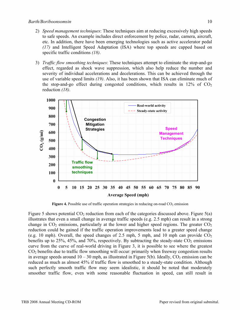
Several important results can be derived from this information, as illustrated in Figure 4:

• In general, whenever congestion brings the average vehicle speed below 45 mph (for a freeway scenario), there is a negative net impact on CO2 emissions. Vehicles spend more time on the road, which results in higher CO2 emissions. Therefore, in this scenario, reducing congestion will reduce CO2 emissions.

• If moderate congestion brings average speeds down from a free-flow speed of about 65 mph to a slower speed of 45 to 50 mph, this moderate congestion can actually lower CO2 emissions. If relieving congestion increases average traffic speed to the free-flow level, CO2 emissions levels will go up.

• Extremely high speeds beyond 65 mph can cause adverse impact on CO2 emissions. If these excessive speeds can be controlled, there will not only be direct safety benefits but also indirect benefits of CO2 reduction.

• If the real-world, stop-and-go velocity pattern of vehicles could somehow be smoothed out so an average speed could be maintained, significant CO2 emissions reductions could be achieved.

Figure 4 shows the potential effect of improved traffic operations on CO2. All of these strategies are important to consider when attempting to reduce CO2 emissions. They can be grouped into three categories as described below:

1) Congestion mitigation strategies: These strategies are focused on increasing average traffic speeds from slower, heavily-congested speeds. Examples include ramp metering and incident management.



2) Speed management techniques: These techniques aim at reducing excessively high speeds to safe speeds. An example includes direct enforcement by police, radar, camera, aircraft, etc. In addition, there have been emerging technologies such as active accelerator pedal (17) and Intelligent Speed Adaptation (ISA) where top speeds are capped based on specific traffic conditions (18).

3) Traffic flow smoothing techniques: These techniques attempt to eliminate the stop-and-go effect, regarded as shock wave suppression, which also help reduce the number and severity of individual accelerations and decelerations. This can be achieved through the use of variable speed limits (19). Also, it has been shown that ISA can eliminate much of the stop-and-go effect during congested conditions, which results in 12% of CO2 reduction (18).

0

100

200

300

400

500

600

700

800

900

1000

0 5 10 15 20 25 30 35 40 45 50 55 60 65 70 75 80 85 90

Average Speed (mph)

CO

2 (g/

mi)

Real-world activitySteady-state activity

Congestion Mitigation Strategies

Traffic flow smoothing techniques

Speed Management Techniques

Figure 4. Possible use of traffic operation strategies in reducing on-road CO2 emission

Figure 5 shows potential CO2 reduction from each of the categories discussed above. Figure 5(a) illustrates that even a small change in average traffic speeds (e.g. 2.5 mph) can result in a strong change in CO2 emissions, particularly at the lower and higher speed regions. The greater CO2 reduction could be gained if the traffic operation improvements lead to a greater speed change (e.g. 10 mph). Overall, the speed changes of 2.5 mph, 5 mph, and 10 mph can provide CO2 benefits up to 25%, 45%, and 70%, respectively. By subtracting the steady-state CO2 emissions curve from the curve of real-world driving in Figure 3, it is possible to see where the greatest CO2 benefits due to traffic flow smoothing will occur: primarily when freeway congestion results in average speeds around 10 – 30 mph, as illustrated in Figure 5(b). Ideally, CO2 emission can be reduced as much as almost 45% if traffic flow is smoothed to a steady-state condition. Although such perfectly smooth traffic flow may seem idealistic, it should be noted that moderately smoother traffic flow, even with some reasonable fluctuation in speed, can still result in



significant CO2 reduction. An example is the application of ISA which reduces CO2 by 12% as compared to a normal driving under congestion (18).

0

10

20

30

40

50

60

70

80

0 5 10 15 20 25 30 35 40 45 50 55 60 65 70 75 80 85 90

Final Speed (mph)

% C

O2 S

avin

g Speed changes 10 mph

Speed changes 5 mph

Speed changes 2.5 mph

Saving as average speed increases

Saving as average speed decreases

(a)

0

10

20

30

40

50

60

70

80

90

100

0 5 10 15 20 25 30 35 40 45 50 55 60 65 70 75 80 85 90

Average Speed (mph)

% D

iffer

ence

(ste

ady-

stat

e as

bas

e)

Greatest CO2 Benefit

from Smoother

Traffic Flow

(b)

Figure 5. Potential CO2 reduction: (a) as a result of speed changes, and (b) as a result of smoother traffic flow

A similar analysis can be performed for travel activities on arterials and residential roads (i.e., interrupted flow patterns). These analyses are relatively more complicated, but they too can be shown that any measure that keeps traffic flowing smoothly for longer periods of time (e.g., operational measures, such as synchronization of traffic signals) can lower CO2 emissions significantly. Also, it is important to note that, although not in the scope of this paper, the CO2 congestion effects will be much more pronounced for heavy-duty trucks, which tend to have much lower power-to-weight ratios than cars.



4. REAL-WORLD CONGESTION

In Section 3 it was shown that CO2 emissions vary greatly depending on average vehicle speed for a variety of vehicle trajectories. Heavy congestion results in slower speeds and greater speed fluctuation, resulting in higher CO2 emissions. On the other hand, traveling at very high speeds also increases CO2 emissions. The best scenario is when traffic as a whole moves at smooth, moderate speeds.

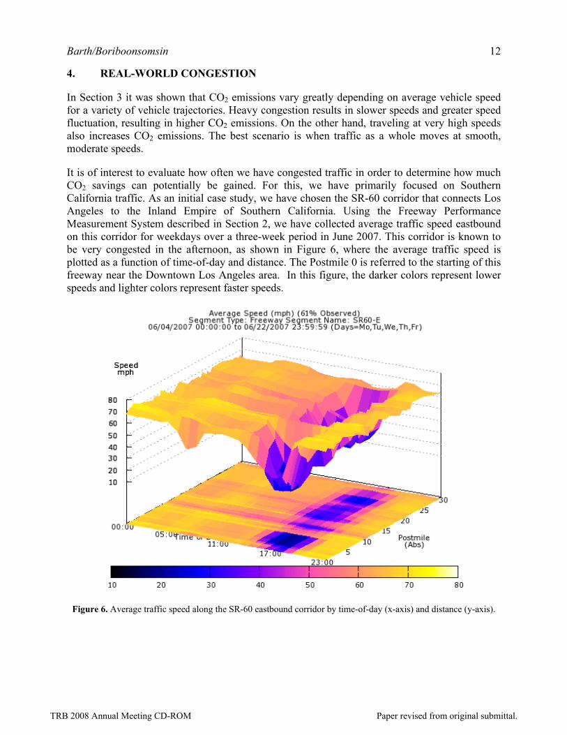
It is of interest to evaluate how often we have congested traffic in order to determine how much CO2 savings can potentially be gained. For this, we have primarily focused on Southern California traffic. As an initial case study, we have chosen the SR-60 corridor that connects Los Angeles to the Inland Empire of Southern California. Using the Freeway Performance Measurement System described in Section 2, we have collected average traffic speed eastbound on this corridor for weekdays over a three-week period in June 2007. This corridor is known to be very congested in the afternoon, as shown in Figure 6, where the average traffic speed is plotted as a function of time-of-day and distance. The Postmile 0 is referred to the starting of this freeway near the Downtown Los Angeles area. In this figure, the darker colors represent lower speeds and lighter colors represent faster speeds.

Figure 6. Average traffic speed along the SR-60 eastbound corridor by time-of-day (x-axis) and distance (y-axis).



Figure 6 shows that the traffic conditions on this corridor vary greatly across different times of the day. Examining the afternoon peak hour only (5-6 p.m.), the VMT-normalized histogram of speeds is shown in Figure 7(a). In this figure, it can be seen that approximately 41% of the VMT that occur during this hour travel at an average speed of 30 mph or lower. It is interesting to see what the impact on CO2 emissions would be if the congestion during this peak hour is relieved. There are different speed thresholds for congestion being used. For example, Caltrans defines congested freeway locations as those where average speeds are 35 mph or less during peak commute periods on a typical incident-free weekday (20). In the TTI’s Urban Mobility Study (3), the congested delay is calculated based on the assumed free-flow speed of 60 mph. In order to provide flexibility in the definition of congestion, PeMS reports several delay numbers, which are calculated based on different threshold values of 35, 40, 45, 50, 55, and 60 mph. For the purpose of estimating potential CO2 reduction in this paper, the congested speed threshold of 60 mph is selected. For this simple case study of Figure 7(a), if this congestion during the peak hour were eliminated so that all VMT were at the average speed of 60 mph, CO2 emissions could be reduced by approximately 7%. Note that the congested speed threshold of 60 mph is intentionally chosen in such a way that the estimated CO2 benefits will be the lower bound. That is, if the threshold is lowered, the CO2 reduction due to congestion mitigation will be even higher. In addition to this particular case study, there are many other freeway corridors throughout Southern California that have similar recurring heavy congestion patterns. Thus, similar CO2 savings could be achieved by moving the average speed distribution towards the distribution with higher speeds.

Looking from an opposing direction, CO2 savings could also be obtained by eliminating extremely high speeds on freeways. These excessive speeds usually occur during off-peak periods, especially at night. Figure 7(b) shows the %VMT-speed histogram of the same corridor during a late night hour (11 p.m. – 12 a.m.). It can be seen that about one-third of the VMT during this hour travel at an average speed of 75 mph or higher. This speeding behavior does not only pose traffic safety concerns but also adversely impacts the environment. Again, assuming that these excessive driving speeds were controlled so that all VMT were at the average speed of 60 mph, CO2 emissions could be reduced by approximately 8%.

It is interesting to point out that when examining the %VMT-speed distribution for the entire freeway network in Los Angeles County for an entire average day, it is found that speeds around 65 to 70 mph dominate, as shown in Figure 8(a). This implies that the freeway system is still operating at a reasonably good condition in overall. However, congestion still occurs, which is relatively small in the distribution compared to the dominant free-flow conditions. This is because the VMT during the peak period (afternoon peak for this case study) account for only a quarter of the total daily VMT, as shown in Figure 8(b). Still, if the traffic flow were managed so that all VMT in Figure 8(a) were at the average speed of 60 mph, CO2 emission from traffic in the Los Angeles freeway network across 24 hours for the month of June 2007 would be almost 5,000 metric tons.

It should be noted that although the presentation in this paper uses traffic in the Los Angeles area as example, the presented concept and methodology are applicable elsewhere. In other areas, the CO2 impact of traffic can be different depending on the following factors:

• Local fleet mix: Different fleet composition will cause different fleet-wide average CO2



emission factors. Therefore, the CO2-versus-speed curves are expected to have different magnitude, and possibly different shape.

• Amount of VMT at congested speed: As presented in the TTI’s Urban Mobility Report, different metropolitan areas have experienced different levels of congestion and delay. Thus, the reduction in CO2 emission that could be achieved may be less in an area where congestion has not been much of a concern.

• Amount of VMT at excessive speed: The amount of driving occurring at excessive speeds is also area-specific. This depends on several factors such as speed limit and enforcement. An area with a lower freeway speed limit is likely to have less CO2 emission due to driving at high speed.

0

10

20

30

40

50

60

5 10 15 20 25 30 35 40 45 50 55 60 65 70 75 80 85 90

Average Speed (mph)

% V

MT

41%

(a)

0

10

20

30

40

50

60

5 10 15 20 25 30 35 40 45 50 55 60 65 70 75 80 85 90

Average Speed (mph)

% V

MT

33%

(b)

Figure 7. %VMT-speed distribution for SR-60 E for the month of June 2007: (a) during the PM peak hour, and (b) during a late night hour



0

10

20

30

40

50

60

5 10 15 20 25 30 35 40 45 50 55 60 65 70 75 80 85 90

Average Speed (mph)

% V

MT

(a)

AM period (6-9 a.m.), 17%

Midday (9 a.m. - 3 p.m.), 32%

PM period (3-7 p.m.), 23%

Nighttime (7 p.m. - 6 a.m.), 28%

(b)

Figure 8. (a) %VMT-speed distribution for Los Angeles freeway network across 24 hours for the month of June 2007, and (b) fraction of total daily VMT for different time periods

6. CONCLUSIONS

It is clear that traffic congestion has a significant impact on CO2 emissions. Overall, even small changes in traffic speed can have significant effect on CO2 emissions. This paper has examined several methods that CO2 can be reduced by improved traffic operations (with particular emphasis on freeway operations). These include:

1) congestion mitigation strategies that reduce severe congestion such that higher average traffic speeds are achieved (e.g. ramp metering, incident management);



2) speed management techniques that can bring down excessive speeds to more moderate speeds of approximately 55 mph (e.g. enforcement, active accelerator pedal); and

3) traffic flow smoothing techniques that can suppress shock waves, and thus, reduce the number of acceleration and deceleration events (e.g. variable speed limits, ISA).

Using a typical traffic condition in Southern California as example, this paper has shown that each of the three methods above could potentially lower CO2 by 7-12%. Although the individual effects may not be that large, the synergistic effect of the three methods combined could add up to a greater amount. Again, these results are considered as a lower bound because they are estimated based on the congested speed threshold of 60 mph. If this threshold was lower, the CO2 reduction could be higher.

While progress in vehicle efficiency improvements and carbon-neutral fuels are underway, innovative traffic operations improvements (i.e. mitigating congestion, reducing excessive speeds, and smoothing traffic flow) can have a significant impact on vehicle CO2 emissions and this impact can be realized in the near-term. In addition to improving traffic operations as a means of reducing vehicle CO2 emissions, other transportation measures can also be simultaneously promoted to reduce VMT, and thus vehicle CO2 emissions. These measures include alternative modes of transportation, innovative land-use patterns, and travel demand-management strategies.

ACKNOWLEDGEMENTS

The authors would like to gratefully acknowledge several students that have been involved in this analysis. Helpful insight has also been provided by David Schonbrunn from the Transportation Solutions Defense and Education fund. This research has partially been funded by a University of California Transportation Center research grant. The contents of this paper reflect the views of the authors and do not necessarily indicate acceptance by the sponsors.

REFERENCES

1. Intergovernmental Panel on Climate Change (2007) “Climate Change 2007: Impacts, Adaptation, and Vulnerability”, Fourth assessment report, April 2007, see http://www.ipcc.ch, accessed July 2007.

2. California Energy Commission (2005) “Options to Reduce Petroleum Fuel Use, Second Edition”, Staff report CEC-600-2005-024-ED2, July 2005.

3. Schrank, D., and T. Lomax (2005) “The 2005 Urban Mobility Report”, Research report, Texas Transportation Institute, Texas A&M University System. Available online at: http://mobility/tamu.edu, accessed July 2007.

4. Barth, M., F. An, T. Younglove, C. Levine, G. Scora, M. Ross, and T. Wenzel. (1999) “The Development of a Comprehensive Modal Emissions Model. Final report submitted to the National Cooperative Highway Research Program, November, 1999, 255 p.


http://www.ipcc.ch/

http://mobility/tamu.edu


5. Fernández, P. C. and Long, J. R. (1995) “Grades and other loads effects on on-road emissions: an on-board analyzer study”, Fifth CRC On-Road Vehicle Emission Workshop, San Diego, April 3-5.

6. Park, S. and Rakha, H. (2006) “Energy and environmental impacts of roadway grades” Proceeding of the 85th Annual Meeting of Transportation Research Board (CD-ROM), Washington, D.C., January.

7. Barth, M., et al., (1996) “Modal Emissions Modeling: A Physical Approach”, Transportation Research Record No. 1520, pp. 81-88, Transportation Research Board, National Academy of Science.

8. Barth, M., T. Younglove, T. Wenzel, G. Scora, F. An, M. Ross, and J. Norbeck (1997) “Analysis of modal emissions from a diverse in-use vehicle fleet”. Transportation Research Record, No. 1587, pp. 73-84, Transportation Research Board, National Academy of Science.

9. Barth, M. T. Younglove, and G. Scora. (2004) “The Development of a Heavy-Duty Diesel Vehicle Model”, Transportation Research Record No. 1880, pp. 10 - 20, Journal of the Transportation Research Board, National Academy of Science.

10. Chen, C, Jia, Z, Petty, K, Shu, J, Skabardonis, A, and Varaiya, P. “Freeway Performance Measurement System (PeMS) Shows Big Picture”, feature article, California PATH Intellimotion, V 9, No. 2, 2000.

11. Choe, T., A. Skabardonis, P. Varaiya. (2002) “Freeway Performance Measurement System (PeMS): An Operational Analysis Tool”, Proceedings (CD-ROM) of the 81st Transportation Research Board Annual Meeting, National Academies, Washington, D.C. January 2002.

12. PeMS, (2007) California Traffic Performance Monitoring System (PeMS), California Department of Transportation, see http://www.calccit.org/projects/pems.html, (accessed January 2007).

13. TRB (Transportation Research Board) (1994) Highway Capacity Manual, Special Report 209. Washington, D.C.: National Academies Press.

14. EPA (Environmental Protection Agency) (1997) “Development of Speed Correction Cycles”, Technical Document #M6.SPD.001, June 1997, prepared by Sierra Research. Washington, D.C.: EPA.

15. Barth, M., Zhu, W., Boriboonsomsin, K., and Ordonez, L. (2007). “Analysis of GPS-based data for light-duty vehicles.” Contract No. 04-327 UCR, Final report to the California Air Resources Board, January, 211 pp.

16. Boriboonsomsin, K. and Barth, M. (2006). “Modeling the effectiveness of HOV lanes at improving air quality.” Contract No. RTA 65A0196, Draft final report to the California Department of Transportation, December, 122 pp.



17. Várhelyi, A., Hjälmdahl, M., Hydén, C., Draskóczy, M. (2004). Effects of an active accelerator pedal on driver behavior and traffic safety after long-term use in urban areas. Accident Analysis and Prevention, 36(5), 729–737.

18. Servin, O., K. Boriboonsomsin, and M. Barth (2006) “An Energy and Emissions Impact Evaluation of Intelligent Speed Adaptation”, Proceedings the 2006 IEEE Intelligent Transportation Systems Conference, Toronto, Canada, September 2006.

19. Oh, J. and Oh, C. (2005). Dynamic speed control strategy for freeway traffic congestion management. Journal of the Eastern Asia Society for Transportation Studies, 6, 595-607.

20. PB study team. HOV Performance Program Evaluation Report. Los Angeles County Metropolitan Transportation Authority, Los Angeles, November 22, 2002.


Real-World CO2 Impacts of Traffic Congestiontransctr/pdf/Barth Article.pdf · Real-World CO2...

Documents

Transcript of Real-World CO2 Impacts of Traffic Congestiontransctr/pdf/Barth Article.pdf · Real-World CO2...