Real-time simulation of dynamic vehicle models ...

Microprocessors and Microsystems 39 (2015) 720–740

Contents lists available at ScienceDirect

Microprocessors and Microsystems

journal homepage: www.elsevier.com/locate/micpro

Real-time simulation of dynamic vehicle models using

a high-performance reconfigurable platform

Madhu Monga, Daniel Roggow, Manoj Karkee1, Song Sun, Lakshmi Kiran Tondehal,Brian Steward, Atul Kelkar, Joseph Zambreno∗

Iowa State University, Ames, IA 50011, USA

a r t i c l e i n f o

Keywords:

FPGA

Real-time simulation

Hardware-in-the-loop

Non-linear functions

Hardware acceleration

a b s t r a c t

With the increase in the complexity of models and lack of flexibility offered by the analog computers, coupled

with the advancements in digital hardware, the simulation industry has subsequently moved to digital com-

puters and increased usage of programming languages such as C, C++, and MATLAB. However, the reduced

time-step required to simulate complex and fast systems imposes a tighter constraint on the time within

which the computations have to be performed. The sequential execution of these computations fails to cope

with the real-time constraints which further restrict the usefulness of Real-Time Simulation (RTS) in a Virtual

Reality (VR) environment. In this paper, we present a methodology for the design and implementation of RTS

algorithms, based on the use of Field-Programmable Gate Array (FPGA) technology. We apply our method-

ology to an 8th order steering valve subsystem of a vehicle with relatively low response time requirements

and use the FPGA technology to improve the response time of this model. Our methodology utilizes tradi-

tional hardware/software co-design approaches to generate a heterogeneous architecture for an FPGA-based

simulator by porting the computationally complex regions to hardware. The hardware design was optimized

such that it efficiently utilizes the parallel nature of FPGAs and pipelines the independent operations. Fur-

ther enhancement was made by building a hardware component library of custom accelerators for common

non-linear functions. The library also stores the information about resource utilization, cycle count, and the

relative error with different bit-width combinations for these components, which is further used to evaluate

different partitioning approaches. In this paper, we illustrate the partitioning of a hardware-based simulator

design across dual FPGAs, initiate RTS using a system input from a Hardware-in-the-Loop (HIL) framework,

and use these simulation results from our FPGA-based platform to perform response analysis. The total simu-

lation time, which includes the time required to receive the system input over a socket (without HIL), software

initialization, hardware computation, and transfer of simulation results back over a socket, shows a speedup

of 2 × as compared to a similar setup with no hardware acceleration. The correctness of the simulation output

from the hardware has also been validated with the simulated results from the software-only design.

© 2015 Elsevier B.V. All rights reserved.

s

d

u

s

t

a

a

1. Introduction

Real-time simulation (RTS) is often a component of virtual proto-

typing used to study the dynamics of a physical system prior to actual

hardware development. It has been utilized by engineers in various

industries such as aviation [1], power systems [2], networking [3], au-

tomotive [4], traffic management [5], and medicine [6]. The physical

∗ Corresponding author. Tel.: +1 5152943312.

E-mail addresses: [email protected] (M. Monga), [email protected]

(D. Roggow), [email protected] (M. Karkee), [email protected]

(S. Sun), [email protected] (L.K. Tondehal), [email protected] (B. Steward),

[email protected] (A. Kelkar), [email protected] (J. Zambreno).1 Present address: Department of Biological Systems Engineering, Washington State

University, USA.

r

e

r

t

u

R

c

w

http://dx.doi.org/10.1016/j.micpro.2015.08.014

0141-9331/© 2015 Elsevier B.V. All rights reserved.

ystems encountered in these areas are mathematically modeled by

eriving the ordinary differential equations (ODEs) that represent the

nderlying physics which dictate system behavior. To simulate these

ystems and estimate their state trajectories across a time duration,

hese ODEs are solved numerically using integration algorithms such

s Runge-Kutta methods, Adams-Bashforth, or Adams-Moulton. The

lgorithms employ either fixed or variable integration time steps. The

esponse generated by the simulation after each time step is consid-

red useful for RTS only if the computation time for each time step

emains below or equal to the actual time being simulated. However,

he general-purpose CPU-based simulation of these systems contin-

es to pose a major limitation on the smallest time-step with which

TS can be achieved. The reduced time-step required to simulate

omplex and fast systems imposes a tighter constraint on the time

ithin which the computations have to be performed. The sequential


http://www.ScienceDirect.com

http://www.elsevier.com/locate/micpro

http://crossmark.crossref.org/dialog/?doi=10.1016/j.micpro.2015.08.014&domain=pdf

mailto:[email protected]









M. Monga et al. / Microprocessors and Microsystems 39 (2015) 720–740 721

Fig. 1. System architecture.

e

c

R

t

a

i

e

t

1

o

w

m

t

t

c

c

b

I

t

a

t

i

a

×o

t

s

d

m

s

a

w

o

i

w

s

e

t

o

a

a

T

t

a

s

s

M

s

t

s

r

s

w

i

s

o

f

f

g

F

t

i

M

t

t

d

e

i

xecution of these computations thus fails to cope with the real-time

onstraints which further restrict the usefulness of RTS in a Virtual

eality (VR) environment.

In this paper, we focus on acceleration of real-time (HIL) simula-

ion of vehicle systems. In our target system, shown in Fig. 1 an oper-

tor provides an input via a physical steering wheel, and the steering

nput is then presented to the vehicle model, after which a graphical

ngine takes the output of the model and renders graphics showing

he movement of the vehicle in a virtual world [7].

.1. Background & motivation

The system of interest for this work is a steering valve subsystem

f a vehicle model. This system is dynamic, since the rates of change

ithin the system affect the response of the system to its environ-

ent [8]. In the steering valve system, for example, the rate at which

he steering wheel is rotated can have significant ramifications on

he direction of the vehicle. The general mathematical model for a

ontinuous-time dynamic system is given in Eq. (1). The mathemati-

al model for such a system must completely define the relationships

etween the system variables [8].

dyi

dt= f (ui, yi) = A ∗ yi + B ∗ ui (1)

n the general form of the equation, yi is an N × 1 vector containing

he state variables, which completely define the state of the system

t an arbitrary instant of time [8]. The response (behavior) of the sys-

em is contained in these variables. The system inputs are contained

n the M × 1 vector ui. Inputs to the system originate externally, and

Fig. 2. Effect of step size and number of states on the CP

re largely independent of the behavior of the system [8]. A is an N

N state transition matrix that defines the coupling between vari-

us states of the system, and B is an N × M input matrix that relates

he system inputs to the system states. A system is linear if all of the

tate and output equations are linear, and take the form of first-order

ifferential equations. Note that this is different from the order of a

odel, which refers to the number of state variables present, e.g. the

teering valve model described in the next subsection has 8 state vari-

bles, so is an 8th order model.

For an initial experiment, a simple and generic linear order model

as implemented in MATLAB using different methods, where it was

bserved that the computation time was negatively affected by the

ncrease in the number of computations involved in solving the ODEs,

hich varies with the choice of numerical integration method, the

ize of the time step t, and the number of physical states N being mod-

led. It is important to note that though an equivalent C implemen-

ation may be faster than a MATLAB implementation, we would still

bserve similar trends, although a more complex method and model

nd a smaller time-step would be needed.

Fig. 2 compares the CPU computation time with various time steps

nd number of states using different numerical integration methods.

he computation time does not include the time required to receive

he steering wheel angle, time to compute the position coordinates,

nd time to send these coordinates to the graphical engine. Fig. 2a

hows the effect of reducing the time step on a 16th order linear

ystem solved using RK1, RK2, RK4, Adams-Bashforth, and Adams–

oulton algorithms. As the time step is reduced, the time taken to

imulate for five seconds increases for a fixed set of design parame-

ers. Eventually, when the time step is reduced below 0.25 ms, the

imulation fails to meet the real-time constraints for all the algo-

ithms, and so further reductions in step size are not possible for this

ystem. Fig. 2b shows the effect of increasing the number of states

ith a fixed time step of size 1 ms. When the number of states is

ncreased to 88, all of the integration algorithms fail to meet the con-

traints, since the overall computation time surpasses the real time

f 5 s. These results motivate our research into alternative platforms

or simulating more complex vehicle dynamics in real-time.

In this work, we explore the reconfigurable capabilities of FPGAs

or accelerating this class of algorithms and design a methodology to

enerate a reconfigurable architecture for different vehicle systems.

PGAs provide a platform to parallelize the independent computa-

ions and a custom pipelined architecture provides an opportunity to

mprove the throughput, though at the expense of an initial latency.

ore work per clock cycle results in a significant improvement in

he computation time, and the reconfigurability allows the platform

o be used for RTS of different vehicle systems without having to

evelop a custom ASIC for the same purpose. We aim to improve the

nd-to-end computation time for vehicle system simulation, which

ncludes everything from the time the simulation model receives the

U computation time for a linear system integrator.

722 M. Monga et al. / Microprocessors and Microsystems 39 (2015) 720–740

c

c

l

s

w

l

c

m

c

o

d

v

u

c

a

m

p

m

c

f

t

t

i

o

v

a

m

d

s

o

l

f

d

I

t

s

T

f

v

s

s

t

m

g

i

d

v

u

v

e

T

v

s

r

s

user input to when the hardware sends the simulation results back

to the display monitor.

The vehicle system targeted for hardware implementation in this

work consists of two subsystems. The first component is a steering

valve subsystem containing the dynamics of a hydraulic system that

uses the steering input to compute the steering angle of the front

wheels of the vehicle. The second component is the vehicle subsys-

tem relating the steering angle to the trajectory of the vehicle as it

is propelled forward at a constant velocity. To simulate the system in

real-time, an integration time step of 10 μs is required for the valve

subsystem simulation and a time step of 2 ms is required for the ve-

hicle subsystem. A CPU-based (MATLAB) simulator was first used to

simulate the whole vehicle system. However, it was observed that the

computation time taken to run the simulation was 13 μs per inte-

gration time step, which fails to meet the 10 μs requirement. Fig. 4a

further describes the main motivation behind our use of FPGA tech-

nology to implement the RTS of the vehicle system. It compares the

computation time of the vehicle system for a simulation period of

five seconds on an FPGA running at 55 MHz, and the single-threaded

MATLAB simulation using the RK4 integration method running on a

2.83 GHz Intel Core 2 Quad CPU. The computation time increases with

an increase in the number of states of the system for both the imple-

mentations. However, for the CPU-based simulator, the computation

time exceeds the real time when the number of states in the system

model is greater than 88. We can intuitively say that a more complex

system with additional subsystems and forces will further add to the

required computation time per iteration and result in the violation of

constraints, even with a fewer number of states.

On the other hand, the computation time for the FPGA-based sim-

ulator remains well below the real-time constraint, since the fine-

grained parallelism present in the model can be extracted using FP-

GAs, which would not be as beneficial using a multicore CPU or

general purpose graphics processing unit (GPGPU). Additionally, the

real-time constraints for this problem make GPGPUs and heteroge-

neous CPU/GPU platforms unsuitable as a targetable solution plat-

form, due to the inherent uncertainty of task scheduling present in

such throughput-oriented architectures [9,10]. Hence, we target an

FPGA platform in this work.

1.1.1. 8th order vehicle system – steering valve and vehicle model

The steering valve dynamics model is this work uses a gerotor

motor and a rotary-valve assembly to direct the fluid to different

branches of a double-ended cylinder. The four valve openings on the

cylinder, two on the left and two on the right, are used to direct flow

to and from the cylinder. The hydraulic dynamics of the rotary-valve

assembly is based on establishing a relationship between the pres-

sure at four different volumes—two in the two sides of the gerotor

motor and two in the two ends of the cylinder—and the net flow rate

(through different valves) to hydraulic volume, given by Eq. (2) [8].

p = β

V× (�Qv) (2)

where p is the pressure, β is the bulk modulus, �Qv is the net flow

rate to volume, and V is the total volume.

The four valves control the flow rate through four openings of the

cylinder. The valve opening area is a function of relative displacement

(rdel) between the angular position of the steering wheel (As) and the

gerotor motor (Am) given by

rdel = As − Am (3)

As is obtained from the continuously changing steering wheel input

from the HIL and Am is computed using the formula

Am = −q1

Ig(4)

where q1 is the derived state of the system and Ig is the gerotor in-

ertia. Since the valve opening area is a function of two dynamically

hanging values As and Am, the flow rate through these valves also

hanges continuously and is computed using the relation given be-

ow:

qrt =√(

2 × abs(pi − p f )

ρ

)Q = A(�) × Cd × sqrt × sign(pi − p f ) (5)

here A(�) is the valve opening area, pi and pf are the inlet and out-

et pressure at the valves, Cd and ρ are the constants that define the

oefficient of discharge and the fluid density, respectively.

The vehicle dynamics of the system is governed by the displace-

ent of a cylinder piston from its neutral position which, in turn, is

ontrolled by the flow rate through valves. The angular displacement

f the piston thus forms the system input for the vehicle model. The

etails of the dynamics of the vehicle model are explained in [7].

Fig. 12 shows the architecture of the vehicle system. The steering

alve model consists of three components: the valve opening area

nit, the orifice flow rate unit, and the state-space solver. The vehi-

le model consists of two components: a trigonometric function and

state-space solver. The non-linear dynamics of the steering valve

odel reads As from the HIL and previous state of the valve to com-

ute the system input for the state-space solver. The solver imple-

ents a numerical integration method, with a time step hvalve, to

ompute the new state of the valve. The state variables model dif-

erent attributes of the valve, and one of the states is used to compute

he system input for the vehicle model using a trigonometric func-

ion. The solver for the vehicle model also implements the numerical

ntegration method with a time step hvehicle. It reads the previous state

f the vehicle and the system input to compute the new state of the

ehicle which is sent to the display monitor.

The valve opening area unit updates the valve opening area of

ll the valves at every time step. For each valve, the maximum and

inimum relative displacement between As and Am is fixed. We

ivide this range into equally spaced values and compute the corre-

ponding area and thereby obtain a look-up table that holds the valve

pening area for predefined relative displacement values. Using a

inear-interpolation method, we can compute the valve opening area

or any value between the given maximum and minimum relative

isplacements.

The orifice flow rate unit updates the flow rate through each valve.

t reads the opening area of the valve A(�), available at the output of

he valve opening area unit, along with the present state yi of the

ystem and computes the flow rate through each valve using Eq. (5).

he inlet and outlet pressure values at the four valves are determined

rom four of the eight states in yi. The flow rate through the four

alves (and two dummy valves which do not affect the state of the

ystem), constant pump outlet pressure (Pp), and As constitute the

ystem input vector for the valve model.

One of the eight states of the steering valve model tracks the pis-

on displacement position after every time step, hvalve. The trigono-

etric function is used to convert the linear displacement to the an-

ular displacement of the piston that eventually forms the system

nput for the vehicle model.

We assume the valve model receives input As every S seconds. To

etermine the final state of the vehicle after S seconds, the steering

alve model is simulated for S/hvalve iterations, followed by the sim-

lation of the vehicle model for S/hvehicle iterations. The input of the

ehicle simulation is either the output of the last iteration, or the av-

rage of all the iterations over S seconds of the steering valve model.

he output of the vehicle model on the last iteration is the state of the

ehicle after S seconds.

The state-space solver for both of the models performs the actual

imulation process by numerically integrating the models at their

espective time steps. These models are in the general form of the

tate-space representation of a linear system, as given in Eq. (1).


Fig. 3. Coefficients and variables for steering valve and vehicle model.

Fig. 4. Motivation and approach.

A

t

r

E

s

m

m

fl

m

c

c

t

c

i

p

v

c

e

r

v

Q

a

r

a

s

v

1

a

v

f

c

s

2

i

lthough the original form of the steering valve model is non-linear,

he required coefficient matrices and vectors for a linear state-space

epresentation of the model were generated using the relation in

q. (2) [11].

The coefficient matrix (A) and state variable vector (yi) for the

teering valve model are shown in Fig. 3a. In A, the first four rows

odel the hydraulic dynamics, where β1 to β4 are the fluid bulk

oduli of the volumes V1 to V4. CL1, CL2, CL3, and CL4 are the leakage-

ow coefficients for each respective volume. CLm is the gerotor

otor leakage-flow coefficient, CLc is the cylinder leakage-flow

oefficient, and Cp is the flow-pressure coefficient for the pipe. The

orresponding state variables are given by p1 to p4.

The next two rows in A model the cylinder piston dynamics, and

he variables are: the cylinder area Ac, the cylinder viscous damping

1, the cylinder spring constant k1, and the gerotor motor moment of

nertia I. The state variables are represented by the velocity (v) and

osition (x) of the cylinder piston.

The last two rows in A represent the gerotor motor and rotary

alve assembly dynamics: the gerotor frictional damping c2, the valve

entering spring constant k2, the gerotor displacement Vd, and the

quivalent mass m of the of steering system. The state variables rep-

esenting the derived states are q1 and q2.

The coefficient matrix (B) and system input vector (ui) for the

ehicle model are shown in Fig. 3b. In the input vector, Qol1, Qol2, and

ol3 are flow rates through the left end of the cylinder, and Qor1, Qor2,

nd Qor3 are flow rates through the right end of the cylinder. The

ows corresponding to flow rates Qol3 and Qor3 in the input matrix B

re zeros, meaning these flow rates do not affect the final state of the

teering valve system, ultimately reducing the number of pressure

alues in the state variable vector for the four valves from 6 to 4.

.2. Paper contributions

We propose a hardware/software co-design approach to acceler-

te the RTS using a heterogeneous parallel architecture. Fig. 4b pro-

ides an overview of our approach. Using this approach, we claim the

ollowing contributions to the state-of-the-art in simulation of vehi-

le system dynamics which otherwise fail to meet the real-time con-

traints using a software (CPU-based) simulator:

• A co-design approach for RTS by partitioning the tasks between a

hardware and a software platform

• A methodology based on an heuristic approach to generate an

FPGA-based simulator. The approach uses a hardware component

library which contains fast hardware implementations of non-

linear functions and timing information of these components

• Application of our methodology to generate the FPGA-based sim-

ulator for the vehicle system and various design strategies ex-

plored based on our methodology

• Proof-of-concept of RTS using a simulator with both hardware and

software components

. Related work

Ever since their genesis in the mid-1980s, FPGAs have been used

n various fields for prototyping, acceleration and reconfigurable


d

h

u

3

b

o

t

a

c

w

m

I

t

w

l

t

r

t

f

t

s

t

v

o

m

o

t

i

d

p

3

r

w

t

(

t

w

a

o

n

A

t

m

t

p

c

p

p

c

o

t

b

i

a

t

t

d

m

computations. [12] outlines the benefits of FPGA implementations in

various fields and the advantages of such reprogrammable systems.

Initially, FPGAs were either used to emulate ASIC-targeted applica-

tions to test the design before the production of custom hardware

[13], or to accelerate computationally intensive applications which

would otherwise have poor performance when implemented in

software. For example, temporal pattern and speech recognition

using a hidden Markov model first compares the digital voice signals

with the English language phonemes to generate a search string.

The search string is then compared with the dictionary words for

the closest match. As the size of the dictionary grows, matching

becomes computationally intensive. The parallel nature of FPGAs

enhances the search process by allowing simultaneous execution of

the independent portions of the design [14]. Other computationally

intensive applications that have been successfully used in parallel ar-

chitectures on the computational fabric of FPGAs are graph problems,

such as finding a Hamiltonian cycle [15], mathematical methods,

such as the finite-difference time-domain method [16] and Jacobi

iteration [17], and, finally, communications decoding algorithms [18].

FPGAs have also played a significant role in the performance

improvement of molecular dynamics (MD) algorithms. MD sim-

ulates the motion and interaction between atoms or molecules

based on different forces acting between these particles. Computing

these forces using a single processor solution is very slow. In 2004,

[19] was the first work published which tested the feasibility of

MD using FPGAs. [20–22] further demonstrate the usefulness and

performance improvement of FPGA-based MD simulations. FPGAs

can also be used in bioinformatics. The earliest such use of hardware

acceleration for biological sequence comparison was in 1998, with a

dedicated hardware accelerator, called SAMBA (Systolic Accelerator

for Molecular Biological Applications) [23]. [24] achieved a speedup

of 200 × over the conventional desktop implementation for protein

sequence alignment, and [25] showed a speedup of 383× for the

multiple DNA sequence alignment problem by implementing the

computationally intensive part of the comparison algorithm on an

FPGA. Because of the significant progress in the field of FPGA-based

acceleration, financial modeling methods have also been ported to

FPGA implementations. [26–28] demonstrate a speedup of up to

80 × for the Monte Carlo simulation algorithm. [29] uses FPGAs for

portfolio management. FPGA-based Gaussian distribution models,

which are used to model correlation between different entities, such

as between portfolios containing hundreds of assets, achieved a

speedup of 33 × over a CPU-based implementation [30].

The use of FPGAs for accelerating real-time simulations of sys-

tems has recently increased. [31,32] implemented a real-time sim-

ulation for permanent magnet synchronous motors using the RT-LAB

real-time simulation platform, as well as auto generated hardware

blocks from Xilinx Simulink Generator (XSG). FPGAs have success-

fully been used to study the dynamic behavior of large power systems

through manual hardware design of a high frequency power sys-

tem simulator. [2] explored a hardware-software codesign approach

for dual time step real-time simulation of power systems. High fre-

quency transient phenomena in power systems can also be simulated

on FPGAs. [33] proposed an FPGA-based real-time electromagnetic-

transient program simulator which is capable of simulating systems

with a time-step of 12 μs, which is well below 50 μs, the mini-

mum required time step for transient simulations. FPGAs thus offer

a promising platform for the simulation of fast transients in power

systems.

Minimal work has been done on accelerating vehicle system dy-

namics using FPGAs. Recently, [34] demonstrated real-time simu-

lation of railway-vehicle dynamics using an FPGA-based accelera-

tor. A fast MATLAB/Simulink implementation of a railway-vehicle

simulator completed each 1 ms time step in 21.5 ms, whereas the

FPGA implementation only consumed 0.625 ms per time step. How-

ever, the time does not include the communication delay due to the

istributed simulation architecture. The rest of this paper details a

ardware/software codesign approach for accelerating real-time sim-

lations of vehicle dynamics.

. Design methodology

In the system-level analysis of Fig. 4b, we determine the partitions

ased on two factors: the computation time of different components

f the simulation model, and the frequency of communication be-

ween different components. To efficiently utilize both the hardware

nd software resources, we obtain an initial partition such that the

omputation-intensive part of the simulation model, and modules

hich can benefit the most by the parallel architecture, are imple-

ented on the hardware, and the rest are implemented in software.

f there is continuous exchange of data between the two partitions,

he increased communication delay between hardware and software

ill negatively affect the overall computation time. The reason for

eaving part of the system in software is twofold: if all of the sys-

em were placed into hardware, a significant amount of hardware

esources would be consumed, and the design may not fit onto the

arget platform. Secondly, the methodology presented in this paper

ocuses on only accelerating in hardware the necessary portions of

he system in order to meet the designer’s real time constraint for

imulation. Software not as critical to the performance of the sys-

em, such as the input controller, can remain in software without ad-

ersely affecting the real-time constraint, which makes maintenance

n those portions easier. Additionally, it is important to note that the

ethodology presented in this paper is not attempting to achieve the

verall optimal performance possible for a hardware/software sys-

em, but to improve the performance only as much as is necessary

n order to meet the real-time constraint as provided by the system

esigner. With these issues in mind, we first discuss the hardware

artitioning followed by software partitioning.

.1. Factors affecting hardware partitioning

Hardware partitioning is governed by three factors: accu-

acy/precision in the simulation results, space occupied on the hard-

are, and the time required to complete the computations of a single

ime step. The accuracy/precision and hardware resource utilization

RU) are affected by the manner in which the data is represented on

he hardware. For this work, we use fixed-point representation [35]

hich consists of a fixed number of integer and fractional bits before

nd after the fixed-point. The accuracy is determined by the number

f integer (I) bits available, whereas the precision is governed by the

umber of fractional (F) bits selected for fixed-point representation.

s the number of bits is increased to improve accuracy/precision in

he simulation results, the space required for the hardware imple-

entation also increases.

The relation between time and space is based on the parallelism

hat can be exploited in the FPGA-based simulator. If all the inde-

endent computations of the CPU-based design are implemented

oncurrently, then the resulting FPGA-based simulator would com-

lete a single iteration in the shortest possible time. However, the

arallelism comes at the expense of hardware resources. Were the

omputation done serially, each component would begin execution

nly after the previous component finishes, and the total computa-

ion time would be the longest. In this case, the hardware RU will

e equivalent to that of the single largest component. A pipelined

mplementation of the design will result in increased throughput,

nd the hardware RU will be somewhere between that of the earlier

wo implementations.

Intuitively, the partitioning between hardware and software for

his type of system follows a pattern that can be extracted into a

esign suitable for a particular system. For example, the underlying

odel in the real-time vehicle simulation system presented in this


Generate fCPU-based

simulatorIs RTE<

RTC

Is RE< PRE?

Decreasebit-width

representationIs RE< PRE?

Choose previous bit-

width representation

Is RU<AR?

Serialize all components

Is RU<AR? Is RTE< RTC?

Stop, Design cannot meet

AR

Parallelizenext smallest component

Is RTE< RTC?

Is RU<AR?Stop, Design cannot meet

AR/RTC

Continue, Generate FPGA-

based design

Stop, Design cannot meet

PRE

Stop, Design can not meet

RTC

Yes

No

NoYesNo

Yes

Yes

No

Yes Yes

No

No

No

NoYes

Yes

Acc

ura

cy &

ti

me

anal

ysis

Sp

ace

&ti

me

anal

ysis

RE: Relative Error AR: Available Resources RTE: Real-Time EstimatePRE: Permissible Range for RE RU: Resource Utilization

1 2

3456

7

8 9 10

11 12 13

Fig. 5. Heuristic approach for hardware partitioning.

p

p

e

s

m

p

t

o

w

a

t

m

a

e

d

3

s

(

a

t

a

f

t

t

3

n

c

h

t

fi

w

r

l

t

s

f

t

t

i

t

d

b

u

o

t

a

a

w

c

t

i

m

c

q

c

f

g

s

m

q

t

l

w

w

n

t

r

aper is, for the most part, linear, and such models have well-known

arallelizable algorithms to compute solutions. Other equations nec-

ssary for the full model definition can be broken down into con-

tituent mathematical functions and operators, which can be imple-

ented using a library of mathematical operations. These individual

ieces can then be joined together to form a hardware implementa-

ion of the computationally intensive portions of the system.

The methodology to generate the FPGA-based simulator, based

n the factors discussed above, is divided into three phases: hard-

are design analysis, hardware design generation and verification,

nd software design analysis. Fig. 5 shows the heuristic approach for

he hardware design analysis phase where we analyze the require-

ents (i.e. the required bit combination, the time taken to complete

single iteration, and the hardware RU). The hardware design gen-

ration phase uses this information to generate the actual hardware

esign.

.2. Hardware design analysis

The input to the hardware design analysis phase is the CPU-based

imulator which uses the RK4 integrator, Permissible Relative Error

PRE) in the simulation output, the Real-Time Constraint (RTC),

nd the available hardware resources (AR). The input is based on

he assumption that the platform is decided in advance, with an

ggressively parallelized design and the maximum number of bits

or fixed-point representation. Ideally, the PRE value should be set by

he engineers who design the simulation model; they should be able

o determine the acceptable relative error in the simulation results.

.2.1. Accuracy/precision and time analysis

Step 1: To implement the methodology described in Fig. 5, we

eed a model which can give us an estimate of the required bit

ombination, the time taken to complete a single iteration, and the

ardware RU. These estimates can be obtained by having a model

hat can emulate the FPGA computation process which we call a

xed-point CPU-based (fCPU-based) simulator. We first design a soft-

are component library containing equivalent software (MATLAB)

epresentations of all the components in the hardware component

ibrary. Each function is implemented using the same techniques

hat are used in the hardware design. The functions in the CPU-based

imulator are then replaced with their modified implementation

rom the software component library. For example, instead of using

he MATLAB built-in ode45 function for integration, we implement

he algorithm for RK4 in MATLAB and use the same algorithm

mplementation for the matching hardware component. In addition,

he arithmetic operations in the modified implementation are also

one using fixed-point notation and are parameterized for different

it combinations. Since the algorithms used are the same as those

sed for hardware implementation, the architecture is close to that

f the FPGA-based simulator. The computation process also emulates

he FPGA computation, thus making the fCPU-based simulator an

ppropriate model to estimate the required bit combination that

ffects the accuracy/precision and the hardware RU.

Step 2: Before we actually generate the design, we estimate

hether the hardware is capable of even meeting the RTC with a

ompletely parallelized design. A parallelized design assumes that all

he independent computations are implemented in parallel, optimiz-

ng for time. Thus, the time obtained from such a design is the esti-

ate of the minimum possible time which the hardware will take to

ompute the output of a single iteration.

The fCPU-based simulator gives us the hardware components re-

uired for the FPGA-based simulator. For each of the independent

omponents in the hardware component library, we use the cycle in-

ormation to compute the number of cycles for the entire design to

enerate the output, accounting for any parallelism used in the de-

ign. Assuming different hardware clock frequencies, we can deter-

ine the Real-Time Estimate (RTE) of this design for these clock fre-

uencies. The RTE is compared against the minimum possible time

hat an FPGA-based simulator will take by exploiting all the paral-

elism in the model. If the RTE is more than the input RTC, the hard-

are will not be able to meet the RTC. If the time taken remains

ithin the RTC, we check for the Relative Error (RE) constraint in the

ext step.

Step 3: In Section 3.1, we discussed that the number of bits affect

he accuracy/precision with which the data values and computation

esults are represented on the hardware. To obtain an estimate of the


0

10

20

30

40

50

60

12 16 20 24 28 32 36 40 44 48 52 56 60 64

Res

ou

rce

uti

lizat

ion

(Th

ou

san

ds

of

AL

Ms)

Integer (I) bits

F=12F=16F=20F=24F=28F=32F=36F=40F=44F=48F=52F=56F=60F=64

Fractional (F) bits

0

2

4

6

8

10

12

14

16

18

20

8 12 16 20 24 28 32 36 40 44 48 52 56 60 64

Res

ou

rce

uti

lizat

ion

(Th

ou

san

ds

of

AL

Ms)

Integer (I) Bits

F=8F=12F=16F=20F=24F=28F=32F=36F=40F=44F=48F=52F=56F=60F=64

Fractional (F) bits

(a) RK4 (b) Look-up Curve

0

10

20

30

40

50

60

70

80

90

100

8 12 16 20 24 28 32 36 40 44 48 52 56 60 64

Res

ou

rce

uti

lizat

ion

(Th

ou

san

ds

of

AL

Ms)

Integer (I) Bits

F=8F=12F=16F=20F=24F=28F=32F=36F=40F=44F=48F=52F=56F=60F=64

Fractional (F) bits

0

2

4

6

8

10

12

16 20 24 28 32 36 40 44 48 52 56 60 64R

eso

urc

e U

tiliz

atio

n(T

ho

usa

nd

s o

f A

LM

s)Integer (I) Bits

F = 16F = 20F = 24F = 28F = 32F = 36F = 40F = 44F = 48F = 52F = 56F = 60F = 64

Fractional(F) Bits

(c) Square Root (d) Trigonometric

Fig. 6. Hardware resource utilization for RK4, look-up curve, square root and trigonometric components.

s

p

t

e

t

b

c

n

c

o

L

i

c

t

u

t

s

t

t

c

w

a

l

a

s

t

c

t

o

r

i

(

t

required bit combination without generating the FPGA-based simula-

tor, we emulate the hardware computation process in the fCPU-based

simulator. This is achieved by converting all the data values at each

computation step into the fixed-point format of length M = I + F bits.

The converted values are equal to, or close to, the true values if the

number of bits is sufficient. The local truncation error due to each

conversion and the global propagation error due to previous conver-

sions result in an error in the final simulation output after every iter-

ation. Since the fCPU-based simulator is generated using algorithms

used for the FPGA-based simulator, the conversion accurately mod-

els the hardware computation process, and the error generated from

this process can be considered a close estimate of the RE that will be

generated from the FPGA-based simulator. If the maximum number

of representation bits produce a RE outside of the PRE constraint, no

suitable hardware partition exists.

Steps 4, 5 and 6: If the constraints are met, we further optimize

the design by reducing the bit-width combination such that the RE

remains within the PRE. We first reduce the number of I bits while

keeping F = 64. After obtaining the number of sufficient I bits, we

reduce the number of F bits until it fails the constraint. However,

the process of estimating the bit-combination using the fCPU-based

simulator is highly dependent upon the number of iterations the

simulation is run. As we increase the number of iterations, the

number of sufficient bits that satisfy the PRE criteria may increase,

so the selected bit-width combination may not be the final estimate

that would represent the values close to the required values on the

hardware.

3.2.2. Space and time analysis

Initially, the timing analysis is performed assuming an aggres-

sively parallelized model, which, if implemented on hardware, would

utilize the maximum available resources. If the optimized design

meets the RTC, it can then be optimized for space to determine if the

model meets the AR constraints.

On the hardware, as the RU increases, the area covered by the de-

sign increases and so does the path traversed by the clock. This in

turn lowers the overall frequency at which the design can run. During
I
pace analysis, we thus optimize the design for space by serializing or

ipelining the components. However, optimizing for space increases

he time taken to run a single iteration.

Before we proceed to the next step, we present our approach to

stimate the hardware RU of the design. The components present in

he hardware component library are independent entities that can

e plugged into any design, as long as the input and output ports are

orrectly mapped. We ran the hardware synthesis for all the compo-

ents in the library and obtained their hardware RU for different bit

ombinations. The results are detailed in Fig. 6. The synthesis was run

n Altera’s Stratix III board, so the RU is in terms of Altera’s Adaptive

ogic Modules (ALMs). An equivalent number of 6-input LUTs on Xil-

nx Virtex-5 FPGAs can be obtained using the relation given in [36].

Step 7: For space analysis, we first check if the design meets the AR

onstraint using the bit-width combination selected in Step 6. We use

he fCPU-based simulator to determine the components that make

p the FPGA-based simulator and use the graphs for resource utiliza-

ion (for some example components) to determine their RU for the

elected combination. We compare the RU for the whole design with

he AR input for the selected platform. If the constraint is met, we use

he automated scripts to generate the VHDL-design for the selected

omponents with the selected bit-width combination. If it does not,

e perform the space optimization and start with a completely seri-

lized design in Step 8.

Steps 8, 9 and 10: In Step 1, we started with an aggressively paral-

elized design (optimized for time), to check for the RTC and obtain

n estimate of the speed-up that can be achieved. To optimize for

pace, we serialize/pipeline the components such that a new compu-

ation starts either after completion of the previous computation or a

ycle later. This process reduces the RU, since the number of compu-

ations done in parallel is reduced. However, to obtain a lower limit

n the hardware RU of the design, we start with a completely se-

ialized design using the selected bit-width combination and check

f this optimized-for-space design is able to meet the AR constraint

Step 9). If the AR constraint cannot be satisfied, then it is impossible

o proceed any further, since the serialized design has the lowest RU.

f the constraint is satisfied, we then check if the new design meets


t

R

a

p

s

s

p

s

s

s

c

t

l

c

R

s

b

c

e

d

a

f

s

t

t

b

t

t

3

e

d

a

r

t

t

e

3

p

v

fi

c

i

b

a

w

r

b

e

o

r

r

3

t

n

t

m

r

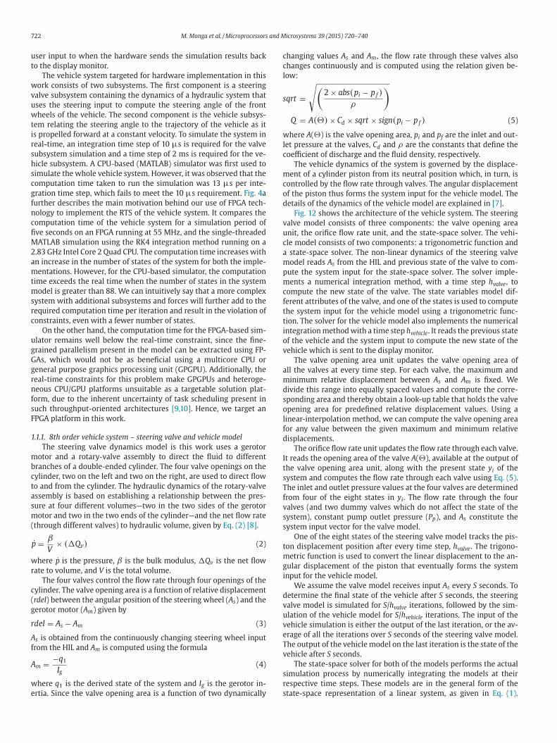
Table 1

Cycle count by individual hardware components.

Component Cycle count

RK4 vehicle 113

RK4 valve 169

Look-up curve 5

Square root 12

Trigonometric 7

a

d

c

I

c

m

w

g

R

s

b

3

l

d

w

h

s

H

s

c

r

u

T

w

s

s

t

i

l

t

a

a

s

s

4

h

i

f

a

p

he RTC (Step 10). As mentioned earlier, the serialization affects the

TE, and, if the completely serialized design meets the RTC, we use

utomated scripts to generate the VHDL design for the selected com-

onents with the selected bit-width combination. If the RTC is not

atisfied, subsequent steps attempt to find a blend of parallelized and

erialized components that meet the constraints.

Steps 11, 12 and 13: In Step 8, we made the assumption of a com-

letely serialized design and obtained the minimum amount of re-

ources consumed by such a design. Since the RTC is not met, while

till optimizing for space, we parallelize the component which con-

umes the minimum resources and thus results in the minimum in-

rease in the overall RU. We check for the RTC in Step 12, and iterate

hrough Step 11 and Step 12 until we meet the RTC. As discussed ear-

ier, as components are parallelized, the RTE decreases but the RU in-

reases. Once the RTC is satisfied, the RU constraint is checked. If the

U constraint still fails, it is impossible to generate an FPGA-based

imulator fulfilling the necessary requirements.

To meet the real-time constraints, the simulation results should

e available at the host for further processing before the RTC is ex-

eeded. This is necessary because the time taken to complete an it-

ration includes both the computation time and the communication

elay. Consequently, the RTE is the sum of the computation time and

communication delay that varies with the amount of data trans-

erred. Therefore, it is necessary to have an interface that provides

ufficient bandwidth and minimizes the latency of data transfer be-

ween the host and the hardware. Since the hardware/software par-

itions have already been decided, the amount of data exchanged

etween the two partitions is known. This information is used to de-

ermine the required bandwidth of the interface and compare it with

he bandwidth of the selected platform.

.3. Hardware design generation and verification

An important aspect of the design methodology is automatic gen-

ration of the design models based on different design decisions. The

esign decisions in this case include the selection of an appropri-

te bit combination that meets the accuracy, time, and space crite-

ia. Such automation is advantageous for designers because it allows

hem to focus on making the best design decisions without devoting

he significant amount of time required for re-creating designs when-

ver a change is necessary.

.3.1. Design generation

The VHDL design for each component is highly parameterized and

ipelined. The parameters for each component, and those specific to

ehicle system simulation, are saved as constants in the parameters

le in fixed-point format based on the bit combination. To use these

onstants, the components need to include the parameters file while

mplementing the design. However, the selection of an appropriate

it combination is an iterative process during which the parameters

nd the VHDL design have to be regenerated. For a complex system

ith numerous components, this step would require the designer to

e-create the design for all of the components every time the bit com-

ination changes. Therefore, to automate the process of design gen-

ration, we designed MATLAB scripts to take the bit combination and

rder of the system (if required) as input, and then generate the pa-

ameters file and VHDL design for the components, including any se-

ialization or pipelining.

.3.2. Design verification

In this step, we compare simulation output from Modelsim with

hat from the CPU-based simulator. Since there are different compo-

ents connected together, it is essential to validate that data from

hese components is represented correctly. Assuming the design

eets the functionality criteria, an insufficient number of bits may

esult in a mismatch of the final simulation output if the output from

ny component is incorrect. After analyzing whether the mismatch is

ue to an insufficient number of I or F bits, we increase the bits ac-

ordingly and go back to Step 7 of the hardware design analysis phase.

n addition to data validation, simulation is an important phase to

heck the speedup that might be expected from the present imple-

entation. Once the Modelsim simulation shows a perfect match

ith the results from the CPU-based simulator, we generate the pro-

ramming file and integrate it with the software design to run the

TS. At this point, it is no longer necessary to run both the CPU-based

imulator and the Modelsim hardware simulator, unless a need to de-

ug the hardware simulator arises later in the design process.

.4. Software design analysis

The software design analysis phase is based on the platform se-

ected because the width of the interface governs the alignment and

ata format in which the system input should be sent to the hard-

are, and the simulation output should be received back from the

ardware. With focus on vehicle system simulation, the software de-

ign should be able to perform the following tasks for the complete

IL RTS:

• Receive the system input from the HIL

• Send the system input to the hardware

• Receive the simulation output from the hardware

• Convert the hexadecimal format of the output to the decimal for-

mat

• Perform software computation, if any

• Send the simulation output to the VR display.

If the system input is assumed to change every T ms, the software

hould be able to perform the above tasks, which includes communi-

ation delays and hardware computation time within this amount of

eal time. The fast computations on the hardware can allow the sim-

lation to complete before the equivalent real-time interval elapses.

hus, to emulate the real-time scenario, we start the timer in the soft-

are just before it receives the system input. The hardware runs the

imulation for T ms and sends the output back to the software and

talls until it receives the new system input. On the software side, the

imer stops after sending the simulation output for further process-

ng. At this point, if the difference between the stop and start timer is

ess than T ms, a sleep command is invoked to stall the software for

he remaining amount of time (i.e. T − (stop − start)).

As the complexity of the simulated physical system increases, the

mount of workload for both the hardware and software partitions

lso increases. To satisfy the RTC, it is essential to develop an efficient

oftware design that minimizes the duration between the start and

top timers.

. Hardware component library

To apply the methodology discussed in Section 3, we developed a

ardware component library of functions required for the hardware

mplementation. Included in our hardware library are components

or look-up curve, square root, and trigonometric functions, as well as

RK4 integrator. Table 1 shows the computation time for each com-

onent in number of clock cycles.


Table 2

Comparison of Xilinx and Altera square root IP cores with our custom square root core.

Xilinx Virtex 7 Altera Stratix IV Altera Stratix III

CORDIC [37] Our worka Floating point [38] Our workb

Data Type Fixed point Fixed point Single precision Fixed point

Latencyc (cycles) 48 2 28 2

I/O Width 48 bits 128 bits 23 bit mantissa 128 bits

Xilinx resource/Altera resource

LUT6 FF pairs/ALUTS 2714 3092 502 2985

LUTs/DLRs 2500 3080 932 632

FFs/ALMs 2511 913 528 1780

Block rams/Memory blocks 0 0 0 0

DSP48E1/DSP18 0 196 –d 272

Max clock (MHz) 283 55 472 55

a Synthesized with the Xilinx tool chain v14.7.b Synthesized with the Altera tool chain v12.1.c Steady state.d Altera does not provide this value.

w

s

t

S

a

s

X

a

X

g

i

w

i

G

t

w

4

p

c

t

s

o

d

i

a

X

I

E

a

m

t

v

g

b

m

w

i

i

The interfaces for each component are very similar to each other,

and to the overall system interface. The whole system behaves simi-

larly to a FIFO queue, and so each component has data input and data

output signals, as well as several control signals to notify components

upstream and downstream of data ready or data needed events.

4.1. Rationale

One method of computing trigonometric and square root func-

tions is to use coordinate rotation digital computer (CORDIC) algo-

rithms. Xilinx takes this approach [37] for their trigonometric and

square root IP core. This core uses fixed point representation and pro-

vides two configurations for implementation: parallel and word se-

rial. A parallel implementation consumes more resources than word

serial, but can produce a result every clock cycle after an initial la-

tency. The word serial implementation can only work on one result

at a time, so has lower throughput.

Another approach is to compute the result using floating point

numbers, and this seems to be the approach Altera uses [38]. Al-

though Altera is sparse on details, floating point implementations in

general tend to have increased complexity and resource usage than

fixed point implementations.

A last approach is to simply use a look-up table and couple it with

a linear interpolation method or use the value as a starting place

for a computation. There are several reasons for selecting a look-

up table approach, including reduced complexity, improved latency

and throughput, and portability between FPGA vendors. However, the

most compelling reason to use a custom look-up table for our system

is because of our special input data width requirements. Our design

requires fixed point inputs of size 128 bits (I and F can each have a

maximum of 64 bits), but Xilinx only supports input widths of up to

48 bits. To overcome these limitations, we developed our own com-

ponents for non-linear functions which support 128-bit input widths.

Table 2 compares our custom square root component with Xilinx and

Altera solutions as a reference. Note that Altera does not provide the

number of DSPs used by their floating point design.

4.2. Look-up curve component

4.2.1. Principle

The look-up curve component estimates the value of a function at

a point input given the value of the function at two precise data points

X1 and X2. It reads the function values at known data points from a

look-up table and uses the linear interpolation method to obtain this

estimate, which is given by the equation below.

Estimate =(

Y2 − Y1

X2 − X1

)× (input − X1) + Y1 (6)

here the input lies between X1 and X2, and Y1 and Y2 are the corre-

ponding function values.

For the hardware implementation, we split the look-up table into

wo tables such that one contains the slope estimate as given by

lope =(

Y2 − Y1

X2 − X1

)(7)

nd the other table contains the corresponding Y values. As we will

ee later, we do not need to store X values, except for the minimum,

min, and maximum, Xmax, since they can easily be computed. Xmin

nd Xmax are saved in the parameters file. For any given input, the two

values between which the input lies is computed using the formula

iven below:

ndex =⌊

input − X0

�X

⌋(8)

here �X is the difference between the equally spaced X values,

nput − X0 determines how far the input is from the first X value, X0.

iven three known values (i.e. input, X0, and �X), we can compute

he index. We use the same formula to compute X1 by replacing input

ith X1. The index is used to compute the read address for both tables.

.2.2. Implementation

In a five stage pipelined architecture, shown in Fig. 7, a valid com-

utation starts when a start signal is received. In the first stage it

hecks if the input is within the maximum and minimum range of

he X values. It also computes the index using Eq. (8). In the second

tage, the index is pipelined for one more stage and the integer bits

f the index are converted to an unsigned format to compute the ad-

ress for reading the two tables. In the third stage, while the memory

s being accessed, we compute X1 using the formula given below, and

lso compute the difference input − X1.

1 = X0 + �X × index (9)

n the fourth stage, we have all the necessary values to compute

q. (6). The value of input − X1 is available from the previous stage,

nd Slope and Y1 are read from the memory. The final output, Esti-

ate, is pipelined for one more stage and is available at the end of

he fifth stage. The pipelined implementation can accept a new input

alue every cycle. After an initial latency of 5 cycles, our component

enerates a new output every cycle.

A two-cycle delay in the computation of the Estimate is avoided

y splitting the look-up tables into two. Furthermore, the imple-

entation is highly parameterized, such that all the parameters

hich do not change during the simulation are saved as constants

n the parameters file. The division by a constant value in Eq. (8) is

mplemented by saving the inverse of �X in this file. When the bit


54321

2 3

1

1

clock

Check range and

compute index

Compute address

andread

memory

Compute estimate

PipelineCompute

x1, input-x1

Index

2

1 2

1 2

4

3

3

5

5

4

3

4

5

4

5

Fig. 7. Pipeline of look-up curve component.

Table 3

Estimated resource utilization of look-up

curve component on an Altera Stratix III

FPGA.

Resource Amount

ALUTs 913

DLRs 641

ALMs 759

DSP18s 54

c

s

f

f

4

t

o

p

p

o

i

s

a

e

s

s

p

b

t

4

a

v

r

b

t

p

u

n

a

x

e√

r

x

y

4

t

a

r

t

2

t

n

t

t

i

o

t

s

a

t

w

t

t

w

i

n

t

p

n

r

n

d

a

e

5

t

T

r

a

ombination changes, the auto-generation scripts for the VHDL de-

ign regenerate these constants and look-up tables in the fixed-point

ormat for the new combination. The estimated resource utilization

or this component is shown in Table 3.

.3. Square-root component

The algorithms to compute the square root in hardware fall into

wo categories: subtractive and multiplicative [39–41]. Subtractive,

r direct methods, are based on the conventional procedure of com-

uting the square-root by hand, where each bit of the result is com-

uted in one clock cycle. This method is efficient for a small number

f input bits, but the initial latency is very high for a larger number of

nput bits. The multiplicative methods (Newton-Raphson and Gold-

chmidt algorithms) on the other hand, iteratively refine the initial

pproximation to compute the square-root. Though the algorithms

xhibit a quadratic convergence, they are expensive in terms of re-

ource utilization. Since our focus is on acceleration of the RTS, where

peed is of prime importance, we chose the latter category for our im-

lementation. The Newton-Raphson method contains dependencies

etween its successive operations, causing an uneven pipeline struc-

ure, thus, we use the Goldschmidt algorithm [42].

.3.1. Principle

The square root function is implemented using the Goldschmidt

lgorithm [42] which is efficient in computing the square root of

alues close to 1. We base our idea on the fact that any number can be

epresented in the form 2n × a, where n is an integer and a is a num-

er close to 1. 2n is the largest power of 2 that appears in the number,

he square root of which is obtained from a look-up table that holds

recomputed square root values. The square root of a is determined

sing the Goldschmidt algorithm. The square root of the original

umber is the product of the two square root values. The Goldschmidt

lgorithm is a three-step process, described in Eqs. (10)–(12) where

and y are set to the initial guess value a. When the process is
0 0
xecuted for several iterations, as xi converges to 1, yi converges to

a.

i = (3 − xi)/2 (10)

i+1 = xi × ri × ri (11)

i+1 = yi × ri (12)

.3.2. Implementation

The look-up table implementation is based on the bit combina-

ion selected for the FPGA implementation. Given the number of I

nd F bits, the maximum and the minimum number that can be rep-

esented as a power of 2 are 2−F and 2I−1, respectively. The look-up

able stores the square root of the following numbers: 2−F , 2−F+1,−F+2, . . . , 20, . . . , 2I−3, 2I−2, 2I−1. To show that the look-up table re-

urns the correct square root value, we introduce 2 index values: the

ormal (n) index and the fixed-point (fp) index. The normal index is

he index interpreted by the hardware for any binary number and also

he address at which to read the look-up table. The fixed-point index

s the index interpreted for fixed-point arithmetic and also the index

f the numbers whose square root values are stored in the look-up

able.

Fig. 8 explains the methodology to obtain the number 2n, its

quare root, and a for computing the square root when number = 2.5

nd with a bit combination of I = 4 and F = 4. In Fig. 8a, the table on

he left-hand side gives binary representation of the number, along

ith index n and index fp values. The table on the right-hand side is

he look-up table generated for the selected bit combination. To de-

ermine the largest power of 2 which is close (and can be represented

ith the given bit combination) to the number, we check index n and

ndex fp corresponding to the first occurrence of 1 in the most sig-

ificant bit (MSB). These values are 5 and 1, respectively. The look-up

able at address 5 stores the square root of 21, which is the largest

ower of 2 that appears in the number. Fig. 8b depicts generating a

umber close to 1, by shifting the number such that the first occur-

ence of 1 in the MSB now lies at the 0th position of the I bits. The

umber of bits to shift is computed by subtracting F bits from the in-

ex n value. If the input is less than 1, index n will be less than F bits

nd the negative difference will shift the input left. A positive differ-

nce will shift the input right. In this case, number is shifted right by

− 4 = 1 bit.

During the first stage of the pipelined architecture, we compute

he address to access the memory where the look-up table is stored.

he address is pipelined in order to be used in the later stages to

ead the memory. The initial guess value, a, for the Goldschmidt

lgorithm is also computed in this stage. r is computed in the second
i


Fig. 8. Methodology to obtain 2n , its square root and a.

s

b

a

w

a

d

p

a

g

a

a

w

s

s

t

0

f

c

t

r

f

r

i

s

l

p

r

u

c

t

b

e

t

o

o

4

s

[

t

w

v

stage. The computation of xi+1 and yi+1 occurs in the third stage. The

Goldschmidt algorithm is executed for five iterations, resulting in a

total runtime of 10 cycles. Since the output from the Goldschmidt

algorithm is not available until end of the 11th stage, a valid read

enable signal is sent to the memory in the 10th stage, along with the

pipelined address value computed in the first stage. By the end of

the 11th stage, we receive the square root of 2n from the memory,

the square root of a from the algorithm, and compute the product

of the two in the final stage. Therefore, the output is available at the

end of the 12th stage. With this pipelined architecture, after an initial

latency of 12 cycles, a valid square root value can be obtained every

other cycle. The estimated resource usage is shown in Table 2.

4.4. Trigonometric function component

4.4.1. Principle

The trigonometric function is implemented using the linear-

interpolation method described in Eq. (6). However, the implemen-

tation is slightly different from the one used for the look-up curve

component. With the linear-interpolation method, a better approx-

imation of the function can be achieved when the interval between

the two precise data points is as small as possible. Though the approx-

imated value gets close to the actual value, an increased number of

data points consumes more FPGA resources. The estimated resource

usage for this component is similar to that of the look-up curve com-

ponent shown in Table 3.

We use the same architecture to compute both the trigonomet-

ric and inverse trigonometric functions. However, the difference is in

the way the input and output data values are interpreted. To com-

pute a trigonometric function, we explore the symmetry among the

function values and generate a look-up table that contains the sine

values for 1250 equally spaced points between the interval 0 to π /2.

The cosine value is generated from the same table using the identity

cos (x) = sin (π/2 − x), and the input is modified accordingly. Also,

the function values in other quadrants can be computed using trivial

trigonometric math, but they may have a different sign. To determine

the sign, we first reduce the input to the component to be in the range

0 to 2π , by computing the floor of the value obtained by division of

the number with 2π . The obtained integer result is multiplied with

2π and then subtracted from the original number. The result is the re-

duced number in the required range. The component determines the

quadrant of the input and the sign, depending on whether it is com-

puting sine or cosine, and reduces the input to the range 0 to π /2.

To compute the inverse trigonometric function, we generate a look-

up table that contains the inverse sine values for 1250 equally spaced

points between the interval 0 to 1. The cosine value is generated from

the same table using the identity arccos (x) = π/2 − arcsin (x).

For a look-up table approach with 1250 points, the principle de-

cribed in Section 4.2, would need two such tables. If the number of

its selected is small, it would be possible to implement a two table

pproach; however, with a large number of bits, the resource usage

ould be tremendous. Thus, we use a single table approach, which

dds a 2 cycle delay to the computation time of the look-up curve

escribed in Section 4.2.

We make two assumptions for the input that is sent to this com-

onent for computing the trigonometric function. Firstly, it is always

positive value. Secondly, it is in the range of 0 to 2π . A number

reater than 2π is converted to a number within this range. For a neg-

tive input value, we compute the two’s complement of the number

nd send the modified value to the component. For the sine function,

e restore the sign by taking the two’s complement of the output,

ince sin ( − x) = − sin (x). For a cosine function, cos ( − x) = cos (x),o a second two’s complement operation is not required. For inverse

rigonometric functions, the input is saturated in the range between

and 1.

The component is fully pipelined to generate a new trigonometric

unction value every cycle after an initial delay of seven cycles. For

omputing inverse trigonometric functions, a reduction of the input

o the range 0 to π /2 is not required. So, in the first stage, we simply

egister the input and compute the index. However, in the first stage

or computing trigonometric functions, a reduction to the required

ange is done before computing the index. In the second stage, the

ndex from the first stage is used to compute the address of two con-

ecutive data points. The third stage does the same arithmetic as the

ook-up curve from Section 4.2.2. In the fourth stage, instead of com-

uting Eq. (6), we compute the difference of the two function values

ead from the memory, and also pipeline the lower index data point

ntil the sixth stage. In the fifth stage, the division of difference by the

onstant �X is implemented by multiplying with its inverse to obtain

he slope estimate. In the sixth stage, the function value is obtained

y computing the product of the result from the fifth stage, the slope

stimate, with the result from the third stage, input − X1, and adding

he result to the lower index data point read from the memory. The

utput is then pipelined for one stage and made available at the end

f the seventh stage.

.5. State-space solver - RK4 integrator

The actual simulation process is performed by solving the state-

pace representation of the system using the RK4 integration method

43], and the steps involved are depicted in Fig. 9. The function f is

he state-space representation of the system described in Eq. (1), and

e use this representation to formulate the dynamics of the steering

alve and vehicle model. The steps involved in the computation of


Fig. 9. Numerical integration using Runge–Kutta methods.

Fig. 10. Data-flow diagram for RK4 iteration.

y

i

a

e

c

i

a

m

t

i

f

t

t

t

t

t

o

t

t

i

d

r

d

a

F

w

n

t

b

c

v

i

t

t

s

c

×l

d

c

t

p

s

r

s

v

i+1 are sequential, since the computation of the new slope (k2, k3, k4)

s dependent on the previous slope (k1, k2, k3). Since we cannot par-

llelize the computations of yi+1, we explore the parallelism within

ach computation. The RK4 integrator for the FPGA-based simulator

onsists of three components: the RK4 controller, the system dynam-

cs, and the system output. The last two components implement the

ctual dynamics of the integrator, and the first component imple-

ents a state machine to control the flow of information between

he other two components. As shown in the data-flow diagram walk-

ng through a single iteration (Fig. 10), each iteration is divided into

our stages. During the four stages, the system dynamics computes

he slope estimate kl (l is the stage number) and feeds the result to

he system output component. The system output computes the in-

ermediate state, yl (except in the last stage), which is fed to the sys-

em dynamics. It also adds and pipelines the intermediate results of

he weight and slope multiplication. In the fourth stage, the system

utput adds these pipelined results and computes the new state of

he system.

We use the parallel architecture of the FPGAs to pipeline compu-

ations within the components in each stage. The system dynamics

mplement matrix-vector multiplication, which is equivalent to z in-

ependent vector–vector multiplications, where z is the number of

ows in a matrix. The architecture of the FPGA gives us the ability to

o these computations in parallel. However, the amount of work that

n FPGA can do in one clock cycle is limited by its clock frequency.

or example, in an Nth order model, a N-by-N matrix is multiplied

ith a N-by-1 vector, where each element is I + F bits long. The total

umber of operations required in one clock cycle are N2 multiplica-

ions and N × N − 1 additions. As the matrix size, or the number of

its, increases, it gets more difficult for the FPGA to perform all these

omputations in one clock cycle. Therefore, we pipeline the matrix-

ector multiplication such that a new vector-vector multiplication is

ssued every cycle. The number of multiplications issued is equal to

he number of rows z in the matrix. Fig. 11a shows different stages in

he vector-vector multiplication of a(1, 1: 8) × y(1: 8, 1) for an 8th order

ystem. Fig. 11b shows the number of cycles taken by the pipeline ar-

hitecture to compute A × y. The matrix-vector multiplication for B

u follows a similar architecture and can be implemented in paral-

el with A × y. However, to improve the timing characteristics of the

esign, we serialize them.

In the six stage pipelined architecture for the system dynamics

omponent, the first stage is used to compute a vector-vector mul-

iplication. In the next stage, the required number of bits from the

roduct are saved in the zeroth vector of a 2D array. In the third

tage, the eight product terms are added using four adders and the

esult is saved in the first vector location of the 2D array. In the fourth

tage, we add these four data values and save the result in the second

ector location. The two data values are summed in the fifth stage. An


Fig. 11. Pipeline architecture of System Dynamics component for an 8th order system.

Valve opening area unit

Orifice flow rate unit

Non-linear dynamics

Steering valve model

Vehicle model

From HIL

To display monitor

Trigonometric function

State-space solver

State-space solver

Fig. 12. Architecture of the vehicle system.

Table 4

Estimated resource utilization of RK4 com-

poncolruent on an Altera Stratix III FPGA.

Resource Amount

ALUTs 3508

DLRs 6410

DSP18s 120

1

n

T

5

e

s

i

w

p

s

w

l

[

c

l

s

T

r

S

5

y

additional stage is used to pipeline the result. For an 8th order system,

each of these stages is implemented for the eight vector-vector mul-

tiplications, so 13 cycles are consumed to compute A × y, as shown in

Fig. 11. The multiplication of B × u also goes through the same stages,

but with an extra stage to sum the result of the two matrix-vector

multiplications, which brings the cycle count to 14 for the second

matrix-vector multiplication. The system output takes 12 cycles

to compute intermediate yl states, and the RK4 controller, which

controls the state transitions, takes another 13 cycles to change states

between the two components. Since there are 4 stages, the total

number of cycles is 4 × 14 + 4 × 13 + 4 × 12 + 13 = 169 clock cycles.

An optimization of this implementation is when the system in-

put u is scalar instead of a vector quantity. In this case, matrix B is a

vector of size N × 1, and B × u is reduced to a vector-vector multipli-

cation. This optimization allows the parallel implementation of the

two multiplications, A × y and B × u, and also reduces the number

of state transitions. The RK4 controller now takes 9 cycles instead of

4, because the two multiplications can be done in parallel. The total

umber of cycles is reduced to 4 × 14 + 4 × 12 + 9 = 113 clock cycles.

able 4 shows the estimated resource utilization for this component.

. Application of the methodology

We use the library of components described in Section 4 to gen-

rate an FPGA-based simulator for an 8th order steering valve sub-

ystem of a vehicle. The steering valve dynamics, described in detail

n [11], simulates the dynamics between the rotation of the steering

heel and the rotational motion of the front wheel about the king

in. The dynamics of this system are quite stiff due to small time con-

tants associated with internal volumes in the steering valve. Thus,

ith RK4, the system is numerically unstable for integration steps

arger than time step hvalve of 10 μs. The vehicle subsystem dynamics

7] that describe the vehicle motion based on steering angle inputs

an be simulated with a time step hvehicle, on the order of a few mil-

iseconds. When implemented in MATLAB, the steering valve model

imulation failed to produce output within the 10 μs time constraint.

he vehicle subsystem, however, when simulated by itself, met its

eal-time constraint. We now apply the methodology discussed in

ection 3.

.1. Application of the methodology

Based on the criteria described in Section 3 for system-level anal-

sis, we implemented the computation intensive part of the model


0

25

50

75

100

125

8 16 24 32 40 48 56 64

Per

cen

tag

e R

E

Fractional (F) Bits

I=48

I=49

I=52

I=56

I=60

I=64

Integer (I) Bits

0.0000.0020.0040.0060.0080.0100.0120.014

40 44 48 52 56 60 64

Per

cen

tag

e R

E

Fractional(F) Bits

I=49

Integer(I) Bits

(a) Relative error for steering valve model

020406080

100120

8 16 24 32 40 48 56 64

Per

cen

tag

e R

E

Fractional (F) Bits

I=8

I=12

I=16

I=20

I=24

Integer (I) Bits

0.000.010.020.030.040.050.06

44 48 52 56 60 64

Per

cen

tag

e R

E

Fractional(F) Bits

I=8

I=12

I=16

I=20

I=24

Integer(I) Bits

(b) Relative error for vehicle model

Fig. 13. Relative error in the output of steering valve and vehicle models.

(

i

c

s

a

t

w

o

s

t

d

b

1

o

u

v

c

t

w

T

t

w

i

m

t

p

l

w

b

t

d

c

v

a

s

t

t

w

fi

n

p

c

o

i

r

r

t

t

a

M

a

1

b

w

I

w

e

w

c

r

t

r

i.e. numerical integration method) in the hardware. The parallelism

n the computations involved in the RK4 method made it an ideal

andidate for FPGA implementation; the method to compute the po-

ition coordinates was simple enough to implement in software. The

mount of communication between the steering valve model and

he vehicle model logically led to the following two possible hard-

are/software partitioning schemes:

• Implement both of the computation-intensive models in hard-

ware, since they can be efficiently parallelized and pipelined, and

then compute the position coordinates in software, or

• Implement the steering valve model in hardware and the vehi-

cle model and position coordinates in software, since the vehicle

model can easily meet the real-time requirements as a software

implementation.

We discuss in detail the first approach and apply the methodol-

gy described in Fig. 5 to the vehicle system discussed above. The

oftware partition and its implementation are discussed along with

he implementation details of the selected hardware. We describe the

esign layout of both implementation strategies in Section 8.

Step 1: The inputs to Step 1 of our methodology were: the CPU-

ased simulator, a PRE of .01%, a RTC for the steering valve model of

0 μs, a RTC of 2 ms for the vehicle model, and 101, 760 × 2 ALMs

f AR (Dual FPGA) [44]. To generate an fCPU-based simulator, we

sed a CPU-based simulator that implemented the dynamics of the

ehicle system and found the functionalities that had an equivalent

omponent in the hardware component library. In our vehicle sys-

em, the valve opening area unit used a linear-interpolation method,

hich was implemented using a hardware look-up curve component.

he orifice flow rate unit used multiplication and square root func-

ions. The multiplications were implemented using on-board hard-

are multipliers, and the square root function was implemented us-

ng a component from the library. The state-space solver for both the

odels used an RK4 component. After choosing the components, all

he equivalent functionalities in the CPU-based simulator were re-

laced with the selected components from the software component

ibrary to obtain the fCPU-based design.

Step 2: For this work, we did not consider the variation in time

ith respect to the number of bits. We assumed that the time taken

y the hardware components remained constant as the bit combina-

ion changed. To estimate the time taken for a completely parallelized

esign, we first enumerated the components in the order required to

omplete a single iteration of both the steering valve model and the

ehicle model. We needed 4 look-up curve components, followed by

pipelined square root component for 6 orifices. The output of the

quare root component was used as input for the RK4 component for

he steering valve model, whose output drove the RK4 component for

he vehicle model. The output from all the look-up curve components

as available after 5 cycles. The implementation of Eq. (5) for 6 ori-

ces took 1 cycle to compute the two’s complement of the negative

umber, 12 cycles to compute the square root, 1 cycle to again com-

ute the two’s complement of the result of the square root, and 1 cy-

le to compute the two multiplications. Thus, the output from all the

rifices was available in 21 cycles. The RK4 components for the steer-

ng valve model and the vehicle model took 169 cycles and 113 cycles,

espectively. An additional 7 cycles were consumed by a trigonomet-

ic function at the input of the RK4 component of the vehicle model

o obtain the angular piston displacement. Thus, a single iteration of

he steering valve model and the vehicle model took 315 cycles. The

mount of time to compute a single iteration for a design with a 100

Hz clock was 3.15 μs; for a design with a 75 MHz clock, 4.2 μs; for

design with a 60 MHz clock, 5.25 μs. Each clock speed satisfied the

0 μs RTC.

Step 3: Ideally, the PRE is determined when the model is built,

ased upon the tolerable amount of error. For our work, the PRE

as .01%. Given the maximum bit-width combination of F = 64 and

= 64, the plots for relative error in Fig. 13 show the PRE constraint

as easily satisfied with this combination.

Steps 4, 5 and 6: We further reduced the bit-width combination by

stimating the relative error for different combinations. We started

ith the maximum bit-width of 128, for which the relative error was

lose to zero. We first estimated the number of I bits for which the

elative error remained within the given PRE value and then reduced

he number of F bits until it satisfied the criteria. Fig. 13a shows the

elative error in the output of the non-linear steering valve model for


Fig. 14. Estimates used for Step 7.

g

w

c

s

t

fi

w

t

h

m

o

c

F

fi

b

I

h

a

A

o

o

w

b

c

I ranging from 64 down to 48 with different values of F. As we re-

duced the number of F bits, the relative error increased until F = 16.

However, for values of F less than 16, the data values were so small

that they were converted to zeros due to insufficient bit-width. As a

result, the relative error decreased to 100% for values of F less than

16. The number of F bits for which the relative error reached an error

value close to the given range was thus estimated to be I = 49 and

F = 42. Similarly, Fig. 13b shows the relative error in the output for

the linear vehicle model for I ranging from 24 down to 8 with differ-

ent values of F. As we reduced the number of I bits, the overlapping

plots imply that the relative error remained constant; whereas it in-

creased as we reduced the number of F bits. The number of F bits

for which the relative error reached an error value close to the given

range was thus estimated to be I = 8 and F = 46.

Step 7: The graphs in Figs. 6 and 14a were used to estimate the

hardware RU for a completely parallelized design. The RU was com-

puted in terms of Altera’s ALMs. The steering valve model needed

four look-up curve components, six square root components, one RK4

component, and a trigonometric function for a total RU of approxi-

mately 98K ALMs. The vehicle model needed one RK4 component for

a RU of approximately 27K ALMs. The total RU was estimated to be

125K ALMs, which was less than the maximum AR of 203.52K ALMs.

Since the PRE constraint was satisfied in Step 6, and the RU was less

than the AR, the selection of hardware/software partitions was suf-

ficient to generate an FPGA design. The parameters file and look-

up tables for each component were automatically configured and

enerated by scripts to use data in fixed-point format with a bit-

idth of M = I + F bits. A wrapper was used to connect the look-up

urve, square root, and RK4 components together.

To check the design for functional correctness, the MATLAB ver-

ion of the design was run for several iterations, and the output af-

er each computation was converted to the equivalent hexadecimal

xed-point representation and logged to a file. Next, the hardware

as simulated using Modelsim for the same number of iterations and

he output compared to the results of the MATLAB simulation. The

ardware simulation using the initial bit-width combination did not

atch the MATLAB output because there were an insufficient number

f F bits needed to represent the small values generated during the

omputations. Therefore, it was necessary to increase the number of

bits and re-iterate through Step 7 until the hardware simulation suf-

ciently matched the MATLAB simulation. The final bit-width com-

ination for the steering valve model was eventually selected with

= 49 and F = 47, and I = 10 and F = 46 for the vehicle model. The

ardware RU then became 113K ALMs for the steering valve model

nd 30K ALMs for the vehicle model, for an approximate total of 143K

LMs, which still satisfied the RU constraint.

The next step was to determine the bandwidth requirement

f the design generated in Step 7. An analysis of the bandwidth

f available communication interfaces on Xilinx and Altera boards

as conducted to find a suitable interface. Fig. 14b depicts the

andwidth requirement of the vehicle model (with only the RK4

omponent) versus the number of model states, as well as the


Fig. 15. Design layout of FPGA-based simulator for the vehicle system.

b

i

G

r

H

t

o

t

b

A

d

h

m

f

a

1

w

s

p

t

a

1

8

f

S

A

w

e

s

v

G

6

d

i

s

f

fl

d

p

o

o

m

r

a

b

p

R

o

F

F

s

s

F

t

p

b

i

1

s

c

o

t

v

m

u

t

t

s

c

i

fi

c

i

i

r

T

andwidth capacities of various interfaces. The interfaces included

n the analysis were: PCIe (2.5 Gb/s) [45], USB (0.48 Gb/s) [46],

igE (1 Gb/s) [47], and FSB (1.035 GB/s) [48]. The plot shows the

equired bandwidth increases as the order of the model increases.

owever, the bandwidth requirement is based upon the amount of

ime necessary to generate the output, so as the computation time

f the model increases, the required bandwidth decreases. Since

he complexity and order of the model increase the amount of time

efore the output is generated, the required bandwidth decreases.

s a result, the bandwidth requirement of the system is expected to

ecrease when the steering valve and vehicle models are combined.

To obtain the required bandwidth for the steering valve and ve-

icle models running at 100 MHz, it was necessary to consider the

aximum amount of data per unit time the FPGA sent and received

rom the CPU. The steering valve model required as inputs 128 bits for

reset signal, 128 × N bits to define the initial state of the system, and

28 bits for the system input. Here, the number of states in the model

as N = 8, so the maximum number of simultaneous data bits neces-

ary for the steering valve model was 1280 bits. Since the system in-

ut was only received once every 20 ms, when the hardware finished

he computation for a given system input, it idled until the next input

rrived. The bandwidth from the CPU to the FPGA was estimated by

280 bits/20 ms = 64 Kb/s. The outputs from the vehicle model were:

states, each 128 bits wide, and a counter value, also 128 bits wide,

or a total of 1152 bits every 20 ms sent from the FPGA to the CPU.

o, the estimated return bandwidth was 1152 bits/20 ms = 57.6 Kb/s.

s Fig. 14b shows, every interface could provide adequate band-

idth for N = 8. Unfortunately, no single-board platform contained

nough resources for the design, so a dual-board solution was cho-

en: the XtremeData platform with two Stratix 3SE260 boards pro-

ided 203.52K ALMs and a bandwidth on the order of 8.28 Gb/s (1.035

B/s).

. Design layout

From the CPU-based simulator, it is clear that the input of one unit

epends upon the output of the previous unit. This sequential flow of

nformation requires that a high-level architecture of the CPU-based

imulator be maintained in the FPGA-based simulator. However, dif-

erences in the architecture of each unit change the way the data-

ow is maintained in the FPGA. Fig. 15 shows how the components

escribed in Section 4 are connected together to construct the data

ath.

For the first implementation strategy, the FPGA-based simulator

f the vehicle system consisted of four major components: the valve

pening area, the orifice flow rate, the state-space solver for the valve

odel, and the state-space solver for the vehicle model. Because of

esource constraints on a single FPGA, we used both FPGAs (FPGA A

nd FPGA B) provided by the XtremeData platform [49]. The shaded

locks in Fig. 15 show the partitioning of the components. FPGA A im-

lements the valve opening area of the steering valve model and the

K4 integrator of the vehicle model, whereas FPGA B implements the

rifice flow rate and the RK4 integrator of the steering valve model.

PGA A is capable of exchanging data with the host and FPGA B, and

PGA B can exchange data only with FPGA A. Each wrapper that in-

tantiates the components on the two FPGAs implements a finite

tate machine (FSM) that synchronizes the data-flow between the

PGAs and the host. Since the interface connecting the two FPGAs

ogether, and FPGA A with the host, is 256 bits wide, the FSMs also

ad the outgoing data with zeros as well as extract the required I + F

its from the incoming data.

The wrapper on FPGA A scans the 32 most significant bits of the

ncoming data packet sent by the host. These bits categorize the first

28 bits of data in the packet as one of the following: simulator re-

et data, system state initialization data, and system input data, re-

eived in that order. When the system input is received, the valve

pening area reads the I + F bits and starts the computation. When

he computation is finished, a “done” signal is asserted, marking the

alidity of the data, and the output vector is padded with zeros to

ake each value 128 bits wide. Each vector contains four 128-bit val-

es, so two packets are required to transmit the entire vector across

he bus. After the transmission completes, the component stalls un-

il it receives new state information from the state-space solver of the

teering valve model. Recall from Eq. (5) that A(θ ) × Cd and sqrt can be

omputed independently of each other. While the valve opening area

s busy computing the former, the system input is also sent to the ori-

ce flow rate to compute the latter. The orifice flow rate stalls after

omputing the sqrt and waits for a valid output from the valve open-

ng area. The wrapper on FPGA B monitors the bus from FPGA A, wait-

ng for a signal to indicate that valid data is available. The valid signal

emains high for two clock cycles, since two 256-bit packets are sent.

he output from the orifice flow rate is a vector of size eight, each


o

s

t

s

r

a

s

a

f

f

C

w

p

E

i

s

t

v

s

m

t

t

t

fi

p

1

a

p

s

t

t

f

i

a

b

1

u

T

o

e

T

s

i

8

t

s

n

s

T

G

B

m

s

d

a

c

b

F

a

s

element I + F bits wide, and a ”done” signal to mark the validity of

the data on the output bus. The orifice flow rate output becomes the

system input for the steering valve state-space solver. The steering

valve model starts computation when the ”done” signal is asserted.

The output from the state-space solver is fed back to both the orifice

flow rate and valve opening area. The orifice flow rate reads all the

states of the system, whereas the valve opening area needs only the

state variable q1 (Fig. 3a).

The vehicle model starts execution only when the steering valve

model has completed. However, because of the difference in their re-

spective time steps, there is not a one-to-one relation between the

number of times each one is executed. When the steering valve model

completes S/hvalve iterations, the vehicle model then runs for S/hvehicle

iterations. Thus, when the state-space solver for the steering valve

completes its execution, the wrapper on FPGA B checks if S/hvalve it-

erations have completed. If not, then the FSM sends the state variable

q1 and x (piston displacement), used to compute the system input

for the state-space solver for the vehicle model, to FPGA A and waits

for the next valid output from the valve opening area. If so, then the

FSM resets the counter to zero and waits for a new system input from

the host to be routed through FPGA A. On FPGA A, a similar check is

made to see if S/hvalve iterations have completed. If so, the trigono-

metric component reads x on the incoming interface from FPGA B,

computes the angular displacement of the piston, and triggers the

vehicle model to run for S/hvehicle iterations. At the same time, the

counter for S/hvalve iterations is reset to 0, and the valve opening area

component is set to wait for a new system input from the host.

The initial state of both the steering valve model and the vehicle

model is assumed to be zero. Thus, when the first system input is

received, the valve opening area does not read the incoming bus from

FPGA B for the updated value of q1. For the next S/hvalve iterations, the

system input remains same, whereas state q1 is updated after every

iteration. The valve opening area component contains four look-up

curve components that read the four different memory blocks where

the data for each valve are stored. The length of the address to access

the memory block is determined by the number of data values in the

block, where each datum is I + F bits long. The information about the

address, maximum and minimum X values in each memory block,

�X, and 1/�X are stored in the parameters files when generating the

VHDL design using the automated scripts.

The orifice flow rate component instantiates a square root com-

ponent, the input of which is the difference between various states of

the valve, determined by the state-space solver. The difference com-

putation is pipelined, so a new input can be sent to the square root

component every cycle. The output from the square-root component

is latched until a valid output is received from the valve opening area.

The system input, u, for the steering valve model is a vector com-

puted by the orifice flow rate component, given in Fig. 13b. The sys-

tem input, u, for the vehicle model is a scalar quantity, computed by

applying a sinusoidal inverse function to the piston displacement, x.

For the vehicle system, the piston displacement is limited to the range

± 0.254, so instead of normalizing the input between 0 and 1, we sat-

urate the input within the given range. A valid ”done” signal triggers

the state-space solver for the vehicle model, which uses the output of

the trigonometric component as system input.

For the second implementation strategy, we implemented the ve-

hicle model in MATLAB and kept the steering valve model on the

FPGA. The previous components were reused, but were put on a sin-

gle FPGA to avoid the communication delay between the FPGAs. The

state-space solver for the vehicle model reads the output of the steer-

ing valve model sent from the FPGA, and then runs for 20 ms.

7. Data flow and cycle estimate

The valve opening area uses the initial two cycles to compute Am

(Eq. (4)) and rdel (Eq. (3)). The division required for the computation

f Am is implemented with an inverse operation. Since Ig remains con-

tant throughout the simulation, its inverse is saved in the parame-

ers file when generating the VHDL design. rdel is computed in the

econd cycle by taking the two’s complement of Am and adding the

esult to As. The look-up curve takes five cycles to generate an output,

cycle to obtain the product with Cd, and a cycle to pipeline the re-

ult. Therefore, a total of 9 cycles are used to obtain the output from

single look-up curve component. Four look-up curve components

or the four valves are instantiated in a pipelined manner, the output

or which is available in 12 cycles. The output for each valve, A(�) ×d, is saved in vector �A(�). An additional cycle is consumed by the

rapper to pad the data with zeros.

The orifice flow rate component reads �A(�), along with the

resent state of the system, yi, and computes the flow rate using

q. (7). Since the product A(�) × Cd was computed by the valve open-

ng area, the orifice flow rate handles two functions of Eq. (5): the

quare root and the multiplication of the square root with �A(�). In

he first cycle, it computes the difference between the two pressure

alues (pi − p f ) by adding the two’s complement of pf to pi. The ab-

olute value of the difference is obtained by taking the two’s comple-

ent only if the difference is negative (i.e the MSB is 1). To replicate

he sign of the difference in the final output from this component,

he sign bit is pipelined for use in a later stage. The square root of

he difference is initiated in the second cycle and takes 12 cycles to

nish. Thus, a single square root computation takes 14 cycles, and a

ipelined architecture for six computations (for six flow rates) takes

9 cycles.

The valve opening area and orifice flow rate are executed in par-

llel. After receiving the new state information from the RK4 com-

onent, the orifice flow rate starts the computation immediately,

talling after 19 cycles, until it receives the latest value of �A(�) from

he valve opening area unit. So, when the valve opening area starts

he computation, the orifice flow rate is already waiting for input

rom the valve opening area unit. The time taken to complete one

teration of the steering valve includes 13 cycles for the valve opening

rea, followed by the 15 cycle delay associated with sending two 256-

it packets to FPGA B. The orifice flow rate takes 8 cycles to complete:

cycle to read the valve area, 6 cycles to compute six flow rate val-

es, and 1 cycle to set up the input vector for the state-space solver.

he state-space solver for the valve model takes 169 cycles, and an-

ther 13 cycles are used to send the two-state output to FPGA A. Thus,

ach iteration of the steering valve model is completed in 226 cycles.

he trigonometric function on FPGA A takes 7 cycles to generate the

ystem input. The state-space solver of the vehicle model reads this

nput and computes the new state in 113 cycles.

. Implementation

The XtremeData XD2000i development system was chosen as the

arget platform for the FPGA-based simulator [49]. The system con-

isted of a development PC with a Xeon dual-processor system, run-

ing the Linux CentOS operating system, and an XD2000i FPGA in-

ocket accelerator that plugged directly into one of the CPU sockets.

he XD2000i module featured three Stratix III EP3SE260 Altera FP-

As: one bridge FPGA and two application FPGAs (FPGA A and FPGA

), each with 254,400 logic elements (101,760 ALMs). The XD2000i

odule connected to the Xeon processor through a 1066 MT/s front-

ide bus (FSB) with a bandwidth of 8.5 GB/s. The bridge FPGA was

edicated to the FSB protocol between the CPU and application FPGAs

nd could not be modified. A 64-bit wide 200 MHz unidirectional bus

onnected the bridge FPGA to the two application FPGAs, and a 256-

it wide 100 MHz bus allowed data to pass between the application

PGAs.

A software controller to manage communication between the CPU

nd the application FPGAs ran on the Xeon processor. The functions to

end and receive data from the application FPGAs were implemented


XD2000i MODULE

AP

P_A

P

OR

T

Bridge FPGA

VALVE OPENING

AREA

APP PORT

APP PORT

ORIFICE FLOW

RK4 Controller

VALVE

256256

64

64

FSB

FSB CORE

FPGA B

FPGA A

BRIDGE PORT

100MHzUnidirectional

Bus at200MHz, DDR

Intel Northbridge

(MCH)

System Memory

RK4 Controller

VEHICLEApplication(CPU)

Fig. 16. XD2000i architecture and application mapping.

a

t

a

e

c

e

t

s

i

D

c

c

s

w

t

a

t

u

i

s

r

F

r

t

h

t

t

9

o

Table 6

Modelsim times for each component.

Component Time (μs)

Steering valve model 4.1

Communication FPGA A → B 0.27

Communication FPGA B → A 0.234

Vehicle model 2.214

RK4 2.05

Trigonometric 0.164

Total 6.818

c

s

m

s

b

2

p

w

O

0

F

o

b

1

c

t

t

t

6

p

s

2

I

k

T

c

s

s

b

2

s

a

s

I

d

s

f

d

s blocking calls to ensure no new data was sent until the results from

he previous transmission were returned. The software controller was

ware of the number of bits a given transaction would send and the

xpected number of bits it would receive. Using this information, the

ontroller created appropriately-sized send and receive buffers. How-

ver, any mismatch between the number of bits sent and received and

he buffer sizes would cause both the controller and the hardware to

tall.

The design partitioning across the two application FPGAs, shown

n Fig. 16 and Table 5, was governed by two factors. First, the Xtreme-

ata platform required both input and output data exchanges to oc-

ur through the same application port. Hence, the valve opening area

omponent, which received the system input, and the state-space

olver of the vehicle model, which generated the simulation output,

ere implemented on the same FPGA. Second, care must be taken

o appropriately divide the hardware components between the two

pplication FPGAs in order to avoid incurring excessive communica-

ion overhead. For example, if the orifice flow rate component, which

tilized the square root core, and the state-space solver for the steer-

ng valve model were implemented on separate FPGAs, the delay re-

ulting from transmitting data for eight states every iteration would

ender the design useless.

The software controller sent the angle of the steering wheel to

PGA A every 20 ms, which allowed the hardware ample time to

eceive the new data, compute the new state of the vehicle, and send

he results back to the CPU. Once the new state was computed, the

ardware simulator stalled until a new input was received, and once

he controller received the new state, it stalled for the remaining

ime.

. Simulation and synthesis results

The FPGA-based vehicle simulator used a time step of 10−6 sec-

nds for hvalve and a time step of 2−3 seconds for hvehicle. The fastest

Table 5

Resource utilization of each component in percentage of ALM

Resource usage Component

RK4 (vehicle)

Valve opening area

Trig. function

RK4 (valve)

Orifice flow

Communication overhead

Input data

Output data

lock at which the design could run and still meet the real-time con-

traints was 55 MHz (18.18 ns period), which was well below the

aximum clock frequency of 100 MHz for the XD2000i platform.

The Modelsim simulator was used to compare the time taken by a

ingle iteration of the simulation on the FPGA with the time taken

y a single iteration of the MATLAB-based simulator running on a

.83 GHz Intel Core2 Quad processor. The MATLAB simulation com-

leted one iteration of the steering valve and vehicle model in 13 μs,

hereas the Modelsim simulation ran the same iteration in 6.818 μs.

f this 6.818 μs, 4.1 μs were consumed by the steering valve model,

.27 μs (15 cycles) were used to send 512 bits of data from FPGA A to

PGA B, and another 0.234 μs (13 cycles) were used to send 256 bits

f data from FPGA B to FPGA A. The total communication overhead

etween the FPGAs was 0.504 μs. Table 6 presents these results.

The vehicle model generated an output in 2.214 μs (123 cycles),

13 cycles of which were consumed by the RK4 component, seven cy-

les by the trigonometric function, 1 cycle to compute the input to the

rigonometric function, and 1 cycle to complement the output of the

rigonometric function. Therefore, the total time for one iteration of

he vehicle simulation in Modelsim was 4.1 + 0.27 + 0.234 + 2.214 =.818 μs, which resulted in a speedup of 2 × over the MATLAB im-

lementation for the same iteration. The Modelsim simulation also

howed that the final output from running the vehicle system for

0 ms (simulator time) would be generated after 9.21 ms (real time).

n other words, the final state of the vehicle after 20 ms would be

nown after just 9.21 ms of real time, which is also a speedup of 2 × .

he time required to send the data over the FSB was negligible when

ompared to the computation time of the model.

A timer was used to measure the execution time of the actual

imulation. The timer starts when the software controller sends the

ystem input to the FPGA and stops after the simulation results have

een received. The measured time was 10 ms, verifying the projected

× speedup over 20 ms. The 10 ms includes the time required to

end the system input to the FPGA, run the simulation on the FPGA,

nd receive the simulation results from the FPGA.

For the second implementation, we were able to implement the

teering valve model on a single FPGA and run the design at 62.5 MHz.

t took 7 ms to simulate 20 ms, excluding a 1 ms communication

elay and 12 ms software stall. The simulation results were then

ent to the vehicle model on the FPGA, which ran the vehicle model

or 20 ms and computed the position coordinates to send to the VR

isplay monitor. Since this second implementation used 3 different

s and communication data overhead.

% FPGA Total

29 A 45%

11 A

5 A

38 B 88%

50 B

Bitwidth Bandwidth (Kb/s)

1280 64

1152 57.6


Fig. 17. Response of the steering valve model to simulated and actual steering input.

Fig. 18. The time for a single iteration of the simulation on different architectures, in microseconds.

t

s

w

s

c

f

platforms to drive the simulation, the simulation lagged slightly, due

to the socket communication delay, which was 16 μs on average. If

the computations were too slow, then, over a period of time, the

accumulated error would cause the vehicle movement in response

to the steering input to become sluggish. To show that the steering

valve model on the FPGA was generating the correct results to pass to

he vehicle model, the piston displacement angles computed by the

teering valve model in response to different steering input sources

ere compared. The first source was a simulated sinusoid and the

econd was the actual steering wheel. Fig. 17 shows the results of this

omparison. The piston displacement angle for the same set of input

rom the MATLAB version of the model was also plotted, and shows


t

t

s

t

e

t

t

i

f

b

1

t

n

u

t

i

d

d

i

f

o

c

W

G

h

F

r

b

w

R

[

[

[

[

[

[

[

[

[

[

[

[

[

[

he MATLAB output overlaps with the FPGA output, further verifying

he correctness of the FPGA steering valve model implementation.

The time taken for a single iteration on different architectures is

hown in Fig. 18. The plot shows that of the three Intel processors,

he Xeon performs the best as the number states increases. How-

ver, all but the slowest-clocked FPGA implementation outperforms

he Xeon at even the smallest number of states. The performance of

he three CPU architectures scales with the number of states approx-

mately linearly, whereas the FPGA architectures scale in a step-wise

ashion. This means that the FPGA solution scales better as the num-

er of states in the system increases.

0. Conclusion

In this paper, we introduced a method to improve the simulation

ime of vehicle systems by using hardware implementations of the

ecessary mathematical models. We presented a methodology based

pon estimating the resource usage of the hardware design early in

he design process in order to make intelligent decisions about the

mplementation strategy. Although the methodology is suitable for

ifferent sizes of models, this paper showed it applied to an 8th or-

er steering valve and vehicle model. The system was successfully

mplemented on a high-performance reconfigurable computing plat-

orm and was able to run the simulation twice as fast as the software-

nly simulator. As a side-effect of this research, a library of hardware

omponents was designed and can now be reused for other models.

hile this paper focused on implementing a model across two FP-

As, the methodology can be formalized to consider any number of

ardware platforms to obtain the best hardware/software partitions.

uture work will focus on improving the existing partitioning algo-

ithms presented in this work, as well as developing algorithms to

etter distribute the components of a model across different hard-

are architectures while still remaining integrated with software.

eferences

[1] S. Zheng, S. Zheng, J. He, J. Han, An optimized distributed real-time simulation

framework for high fidelity flight simulator research, in: Proceedings of Interna-

tional Conference on Information and Automation (ICIA), 2009, pp. 1597–1601,doi:10.1109/ICINFA.2009.5205172.

[2] P. Le-Huy, S. Guerette, L. Dessaint, H. Le-Huy, Dual-step real-time simulation ofpower electronic converters using an FPGA, in: Proceedings of IEEE International

Symposium on Industrial Electronics, 2006, pp. 1548–1553.[3] X. Xiaobo, Z. Kangfeng, Y. Yixian, X. Guoai, A model for real-time simulation of

large-scale networks based on network processor, in: Proceedings of the Broad-

band Network Multimedia Technology (IC-BNMT), 2009, pp. 237–241, doi:10.1109/ICBNMT.2009.5348486.

[4] M. Tavernini, B. Niemoeller, P. Krein, Real-time low-level simulation of hybrid ve-hicle systems for hardware-in-the-loop applications, in: Proceedings of Vehicle

Power and Propulsion Conference (VPPC), 2009, pp. 890–895, doi:10.1109/VPPC.2009.5289753.

[5] J. Maroto, E. Delso, J. Felez, J. Cabanellas, Real-time traffic simulation with a micro-

scopic model, IEEE Trans. Intell. Transp. Syst. 7 (4) (2006) 513–527, doi:10.1109/TITS.2006.883937.

[6] M. Lerotic, S.-L. Lee, J. Keegan, G.-Z. Yang, Image constrained finite element mod-elling for real-time surgical simulation and guidance, in: Proceedings of Biomed-

ical Imaging: From Nano to Macro, 2009, pp. 1063–1066, doi:10.1109/ISBI.2009.5193239.

[7] M. Karkee, B.L. Steward, Open and closed loop system characteristics of a tractor

and an implement dynamic model, in: Proceedings of the Annual Meeting of theAmerican Society of Agricultural and Biological Engineers (ASABE), 2008.

[8] B.T. Kulakowski, J.F. Gardner, J.L. Shearer, Dynamic Modeling and Control of Engi-neering Systems, 3rd, Cambridge University Press, 2007.

[9] H. Zhou, G. Tong, C. Liu, GPES: a preemptive execution system for GPGPU comput-ing, in: IEEE Real-Time and Embedded Technology and Applications Symposium

(RTAS), 2015, pp. 87–97, doi:10.1109/RTAS.2015.7108420.

[10] C. Liu, J. Anderson, Suspension-aware analysis for hard real-time multiprocessorscheduling, in: Proceedings of the Euromicro Conference on Real-Time Systems

(ECRTS), 2013, pp. 271–281, doi:10.1109/ECRTS.2013.36.[11] M. Karkee, Real-time simulation and visualization architecture with field pro-

grammable gate array (FPGA), in: Proceedings of the ASME World Conference onInnovative Virtual Reality (WINVR), 2010.

[12] S. Hauck, The roles of FPGAs in reprogrammable systems, Proc. IEEE 86 (4) (1998)

615–638, doi:10.1109/5.663540.

[13] S. Note, P. van Lierop, J. van Ginderdeuren, Rapid prototyping of DSP systems:requirements and solutions, in: Proceedings of IEEE International Workshop on

Rapid System Prototyping, 1995, pp. 88–96, doi:10.1109/IWRSP.1995.518576.[14] H. Schmit, D. Thomas, Hidden markov modeling and fuzzy controllers in FPGAs,

in: Proceedings of IEEE Symposium on FPGAs for Custom Computing Machines,1995, pp. 214–221, doi:10.1109/FPGA.1995.477428.

[15] M. Serra, K. Kent, Using FPGAs to solve the hamiltonian cycle problem, in: Pro-ceedings of the International Symposium on Circuits and Systems (ISCAS), 2003,

pp. 228–231.

[16] J. Durbano, F. Ortiz, FPGA-based acceleration of the 3d finite-difference time-domain method, in: Proceedings of IEEE Symposium on Field-Programmable Cus-

tom Computing Machines (FCCM), 2004, pp. 156–163, doi:10.1109/FCCM.2004.37.

[17] G. Morris, V. Prasanna, An FPGA-based floating-point Jacobi iterative solver, in:Proceedings of International Symposium on Parallel Architectures, Algorithms

and Networks (ISPAN), 2005, p. 8, doi:10.1109/ISPAN.2005.18.

[18] B. Pandita, S. Roy, Design and implementation of a viterbi decoder using FPGAs,in: Proceedings of the International Conference on VLSI Design, 1999, pp. 611–

614, doi:10.1109/ICVD.1999.745223.[19] N. Azizi, I. Kuon, A. Egier, A. Darabiha, P. Chow, Reconfigurable molecular dynam-

ics simulator, in: Proceedings of Field-Programmable Custom Computing Ma-chines (FCCM), 2004, pp. 197–206, doi:10.1109/FCCM.2004.48.

20] J.-H. Kim, C.-S. Park, S.-G. Kim, J.-H. Kim, Improved interpolation and system inte-

gration for FPGA-based molecular dynamics simulations, in: Proceedings of Inter-national Conference on Field Programmable Logic and Applications (FPL), 2006,

pp. 21–28.[21] R. Scrofano, M.B. Gokhale, F. Trouw, V.K. Prasanna, A hardware/software approach

to molecular dynamics on reconfigurable computers, in: Proceedings of the 14thAnnual IEEE Symposium on Field-Programmable Custom Computing Machines

(FCCM), 2006, pp. 23–34.

22] Y. Gu, T.V. Martin, C. Herbordt, FPGA-based multigrid computation formolecular dynamics simulations, in: Proceedings of IEEE Symposium on Field-

Programmable Custom Computing Machines (FCCM), 2007, pp. 117–126.23] D. Lavenier, Speeding up genome computations with a systolic accelerator,

1998, http://www.irisa.fr/symbiose/lavenier/Publications/Lav98ja.pdf (accessedJune 2015).

[24] S. Dydel, Large scale protein sequence alignment using FPGA reprogrammable

logic devices, in: Proceedings of International Conference on Field ProgrammableLogic and Application (FPL), 2004, pp. 23–32.

25] A. Boukerche, J. Correa, A. de Melo, R. Jacobi, A. Rocha, An FPGA-based acceleratorfor multiple biological sequence alignment with DIALIGN, in: High Performance

Computing (HiPC), in: Lecture Notes in Computer Science, 4873, Springer Berlin /Heidelberg, 2007, pp. 71–82.

26] G. Zhang, P. Leong, C. Ho, K. Tsoi, C. Cheung, D.-U. Lee, R. Cheung, W. Luk, Recon-

figurable acceleration for Monte Carlo based financial simulation, in: Proceed-ings of International Conference on Field-Programmable Technology (FPL), 2005,

pp. 215–222, doi:10.1109/FPT.2005.1568549.[27] D.B. Thomas, J.A. Bower, W. Luk, Automatic generation and optimisation of re-

configurable financial monte-carlo simulations, in: Proceedings of InternationalConference on Application-specific Systems, Architectures and Processors (ASAP),

2007, pp. 168–173.28] N. Woods, T. VanCourt, FPGA acceleration of quasi-Monte Carlo in finance, in:

Proceedings of International Conference on Field Programmable Logic and Appli-

cations (FPL), 2008, pp. 335–340, doi:10.1109/FPL.2008.4629954.29] A. Irturk, B. Benson, N. Laptev, R. Kastner, FPGA acceleration of mean variance

framework for optimal asset allocation, in: Proceedings of Workshop on High Per-formance Computational Finance (WHPCF), 2008, pp. 1–8.

30] D.B. Thomas, W. Luk, Sampling from the multivariate Gaussian distributionusing reconfigurable hardware, in: Proceedings of IEEE Symposium on Field-

Programmable Custom Computing Machines (FCCM), 2007, pp. 3–12.

[31] C. Dufour, S. Abourida, J. Belanger, Real-time simulation of permanent magnetmotor drive on FPGA chip for high-bandwidth controller tests and validation,

in: Proceedings of IEEE International Symposium on Industrial Electronics, 2006,pp. 2591–2596, doi:10.1109/ISIE.2006.295980.

32] C. Dufour, J. Belanger, S. Abourida, V. Lapointe, FPGA-based real-time simulationof finite-element analysis permanent magnet synchronous machine drives, in:

Proceedings of Power Electronics Specialists Conference (PESC), 2007, pp. 909–

915, doi:10.1109/PESC.2007.4342109.[33] Y. Chen, V. Dinavahi, FPGA-based real-time EMTP, IEEE Trans. Power Deliv. 24 (2)

(2009) 892–902, doi:10.1109/TPWRD.2008.923392.34] Y. Zhou, T. Mei, S. Freear, Field programmable gate array implementation of

wheel-rail contact laws, Control Theory Appl., IET 4 (2) (2010) 303–313, doi:10.1049/iet-cta.2008.0601.

[35] R. Yates, Fixed-point arithmetic: an introduction, 2007, http://www.

digitalsignallabs.com/fp.pdf (accessed June 2015).36] A. Percey, Advantages of the Virtex-5 FPGA 6-Input LUT Architecture,

2007, http://www.xilinx.com/support/documentation/white_papers/wp284.pdf(accessed June 2015).

[37] Xilinx, LogiCORE IP CORDIC (DS858), 2011, V5.0.38] Altera, Floating-Point IP Cores User Guide (UG-01058), 2014.

39] P. Montuschi, P. Mezzalama, Survey of square rooting algorithms, IEEE Proc. Com-

put. Digital Tech. 137 (1) (1990) 31–40.40] P. Soderquist, M. Leeser, An area/performance comparison of subtractive and

multiplicative divide/square root implementations, in: Proceedings of the Sym-posium on Computer Arithmetic, 1995, pp. 132–139, doi:10.1109/ARITH.1995.

465366.

http://dx.doi.org/10.1109/ICINFA.2009.5205172

http://refhub.elsevier.com/S0141-9331(15)00147-7/sbref0002





http://dx.doi.org/10.1109/ICBNMT.2009.5348486

http://dx.doi.org/10.1109/VPPC.2009.5289753

http://dx.doi.org/10.1109/TITS.2006.883937

http://dx.doi.org/10.1109/ISBI.2009.5193239








http://dx.doi.org/10.1109/RTAS.2015.7108420

http://dx.doi.org/10.1109/ECRTS.2013.36



http://dx.doi.org/10.1109/5.663540

http://dx.doi.org/10.1109/IWRSP.1995.518576

http://dx.doi.org/10.1109/FPGA.1995.477428




http://dx.doi.org/10.1109/FCCM.2004.37

http://dx.doi.org/10.1109/ISPAN.2005.18

http://dx.doi.org/10.1109/ICVD.1999.745223

http://dx.doi.org/10.1109/FCCM.2004.48















http://www.irisa.fr/symbiose/lavenier/Publications/Lav98ja.pdf









http://dx.doi.org/10.1109/FPT.2005.1568549





http://dx.doi.org/10.1109/FPL.2008.4629954









http://dx.doi.org/10.1109/ISIE.2006.295980

http://dx.doi.org/10.1109/PESC.2007.4342109

http://dx.doi.org/10.1109/TPWRD.2008.923392

http://dx.doi.org/10.1049/iet-cta.2008.0601

http://www.digitalsignallabs.com/fp.pdf

http://www.xilinx.com/support/documentation/white_papers/wp284.pdf




http://dx.doi.org/10.1109/ARITH.1995.465366


B

iE

nc

Mc

wt

f

t

[41] G. Cappuccino, P. Corsonello, G. Cocorullo, High performance VLSI modules fordivision and square root, Microprocess. Microsyst. 22 (5) (1998) 239–246, doi:10.

1016/S0141-9331(98)00082-9.[42] P. Soderquist, M. Leeser, Division and square root: choosing the right implemen-

tation, IEEE Micro 17 (4) (1997) 56–66, doi:10.1109/40.612224.[43] Chapra, Canale, Numerical Methods for Engineers, 5th, Tata McGraw-Hill, 2006.

[44] M. Karkee, Modeling, identification and analysis of tractor and single axle towedimplement system, Iowa State University, 2009 (Ph.D. thesis). Paper 10875.

[45] PCI Express Base Specification, PCI-SIG, 2007. Rev. 2.0.

[46] Compaq, Hewlett-Packard, Intel, Lucent, Microsoft, NEC, Philips, Universal SerialBus Specification, 2000. Rev. 2.0.

[47] IEEE Standard for Ethernet, IEEE, 2008.[48] XtremeData, Xd2000iTMdevelopment system, http://www.altima.co.jp/products/

xtremeData/download/XD2000i_PF_WEB.pdf (accessed June 2015).[49] XtremeData, Xd2000iTMdevelopment system, (accessed June 2015).

Madhu Monga received her B.S. degree in Electronics and

Communication from Kurukshetra University in 2003, andher M.S. degree in Electrical and Computer Engineering

from Iowa State University in 2010. She was a research as-sistant in the Reconfigurable Computing Lab until 2010 and

worked on accelerating real-time simulation of dynamicsystems. She is currently employed at Algo-Logic. Her re-

search interests include high performance reconfigurable

computing and embedded systems.

Daniel Roggow received his B.S. degree in Computer Engi-

neering from Iowa State University, Ames, IA, in 2014. Heis currently a research assistant working on his Ph.D. in the

Reconfigurable Computing Laboratory at Iowa State. His re-search interests include reconfigurable computing and em-

bedded systems.

Manoj Karkee is an assistant professor in the Biological

Systems Engineering Department. Dr. Karkee was born inNepal where he received his undergraduate degree in Com-

puter Engineering. He went to Asian Institute of Technol-ogy, Bangkok, Thailand in 2003 for his Master’s Degree in

Remote Sensing and GIS. He received his Ph.D. in Agricul-

tural Engineering and Human Computer Interaction fromIowa State University in 2009 and joined WSU in 2010.

Dr. Karkee has established a strong research program inagricultural automation and mechanization area with par-

ticular emphasis on machine vision systems. Some of hissponsored projects include crop load estimation, fruit tree

pruning, plant stress monitoring, and solid set canopy de-

livery. He has been publishing actively in journals such as ‘Computers and Electronicsin Agriculture’, and ‘The Transactions of ASABE’ and has been presenting frequently in

national and international conferences.

Song Sun received his B.S. degree in Computer Science andEngineering from the Beijing Information Technology In-

stitute in 1998, his M.S. degree from the University of Sci-

ence and Technology of China in 2001, and his Ph.D. degreein Electrical and Computer Engineering from Iowa State

University, Ames, IA, in 2011. He currently is working atthe Symantec Corporation. His research interests include

high performance reconfigurable computing and embeddedsystems.

Lakshmi Kiran Tondehal received her B.S in Electronics

and Instrumentation from the Birla Institute of Technol-ogy and Science (BITS) Pilani, Goa campus in 2009, and her

M.S. in Electrical and Computer Engineering from Iowa State

University, Ames IA in 2011. Her research interests are inembedded systems, reconfigurable computing and VlSI de-

sign. She is currently a Memory Product Engineer at MicronTechnology, Boise ID.

Brian Steward is Professor of Agricultural and BiosystemsEngineering at Iowa State University. Dr. Steward teaches

in the areas of dynamic systems modeling and simulation,fluid power engineering and technology, computational in-

telligence, and sustainable engineering. His research fo-

cuses on the areas of dynamic systems and sensing foragriculture and biosystems, precision agriculture, and field

automation and mechatronics at the interface of machineand environment. He provides leadership to international

programs within the ABE Department including coordina-tion of student exchange programs with Federal University

of Viçosa, Viçosa, Minas Gerais, Brazil, Federal University ofCampina Grande, Paraiba, Brazil and study abroad trips to

razil. He is a member of the American Society of Agricultural and Biological Engineers

n which he been an associate editor for seven years and currently chairs the Resourceditorial Board. He has a total of 177 technical publications including 35 refereed jour-

al articles and 44 invited talks. He has received more than $4.8 million in grants andontracts as a principal investigator or co-principal investigator. He received his BS and

S in Electrical Engineering from South Dakota State University, and his Ph.D. in Agri-ultural Engineering from the University of Illinois at Urbana-Champaign.

Atul Kelkar is a Professor of Mechanical Engineering atIowa State University and prominent scholar in the area of

Dynamic Systems and Control. Dr. Kelkar received his Ph.D.degree in Mechanical Engineering from Old Dominion Uni-

versity, Norfolk, Virginia, in 1993 while working as a Re-search Scientist at NASA Langley Research Center, Hampton,

VA. Dr. Kelkar joined Iowa State University in 2001 and cur-rently holds the position of Professor in Mechanical Engi-

neering Department.

Joseph Zambreno (M ’02) received his B.S. degree (Hons.)

in Computer Engineering in 2001, his M.S. degree in Electri-

cal and Computer Engineering in 2002, and his Ph.D. degreein Electrical and Computer Engineering from Northwestern

University, Evanston, IL, in 2006. Currently, he is an Assis-tant Professor in the Department of Electrical and Com-

puter Engineering at Iowa State University, Ames, wherehe has been since 2006. His research interests include

computer architecture, compilers, embedded systems, and

hardware/software co-design, with a focus on run-time re-configurable architectures and compiler techniques for soft-

ware protection. Dr. Zambreno was a recipient of a NationalScience Foundation Graduate Research Fellowship, a North-

estern University Graduate School Fellowship, a Walter P. Murphy Fellowship, andhe Electrical Engineering and Computer Science Department Best Dissertation Award

or his Ph.D. dissertation “Compiler and Architectural Approaches to Software Protec-

ion and Security”.

http://dx.doi.org/10.1016/S0141-9331(98)00082-9

http://dx.doi.org/10.1109/40.612224






http://www.altima.co.jp/products/xtremeData/download/XD2000i_PF_WEB.pdf

Real-time simulation of dynamic vehicle models ...

Documents

Transcript of Real-time simulation of dynamic vehicle models ...