Real Time Risk Management: An AAD-PDE Approach Capriotti.pdf · Real Time Risk Management: An...

Real Time Risk Management: An AAD-PDE Approach

Luca Capriotti†,?, Yupeng Jiang?, Andrea Macrina?

† Quantitative Strategies, Credit Suisse? Department of Mathematics, University College London

HPCFinance 2016London, March 14-15, 2016

The opinions and views expressed in this presentation are uniquely those of the authors, and do

not necessarily represent those of Credit Suisse Group.

L. Capriotti, Y. Jiang, A. Macrina Real Time Risk Management with AAD-PDE 1 / 35

Disclaimer


Outline

‘Bump and Reval’ is sooo ’90s

Risk for the 2010’s: Adjoint Algorithmic Differentiation (AAD)

AAD and Partial Differential Equations (Backward and Forward)

Calibration and Implicit Function Theorem

Conclusions




I The calculation of risk by means of standard ‘bump and reval’ (orbumping) techniques is not sustainable in the modern financialenvironment because of the high computational cost associated withrisk management practices emerged in the aftermath of the financialcrisis.

I Multi curve framework for interest rates, collateral adjusteddiscounting, XVA etc. all translate in a significant increase of thecomputational costs and of the number of price sensitivities that needto be computed.

I In order to complete risk calculations in a practical amount of time,financial firms employ vast amounts of computational resources(standard CPUs/ FPGAs/ GPUs) bearing an high infrastructure cost.

I Solving this technology problem is of paramount importance for asecurities firm to remain competitive.



Risk for the 2010’s: Adjoint Algorithmic Differentiation(AAD)

I Adjoint Algorithmic Differentiation (AAD) is a recently introducedtechnology for real time risk:

I L. Capriotti, Fast Greeks by Algorithmic Differentiation, J. of Comp.Finance 14, 3 (2011).

I L. Capriotti and M. Giles, Algorithmic Differentiation: adjoint Greeksmade easy, Risk 25, 95 (2012).

I L. Capriotti, US Patent 9058449B2.I See also the Risk Magazine Editorials:

I Credit Suisse: Algorithmic Gymnastic, Risk Magazine 2012.I Maths versus Machine, Risk Magazine 2014.I Chips off the Menu. AAD vs GPUs: banks turn to maths trick as chips

lose appeal, Risk Magazine 2015.

I AAD allows the fast computation of risk without the necessity ofrepeating the valuation of the portfolio multiple times as in traditionalbump and reval approaches.



Adjoint Algorithmic Differentiation (AAD)

I In contrast to computational solutions based on parallel architectureslike GPUs and FPGAs, AAD does not require investments in newinfrastructure or additional computational resources. Rather, AAD isa straightforward mathematical technique that can be easilyimplemented and integrated in existing analytics software.

I The remarkable efficacy of AAD was demonstrated in a variety of riskmanagement problems in the context of highly time consuming MonteCarlo valuations, including counterparty credit management, see e.g.:

I L. Capriotti and M. Giles, Fast Correlation Greeks by AdjointAlgorithmic Differentiation, Risk Magazine 23, April (2010).

I L. Capriotti, M. Peacock, and J. Lee, Real Time Counterparty CreditRisk in Monte Carlo, Risk Magazine 24, 86 (2011).




I Algorithmic Differentiation (AD) aims at computing accurately andefficiently the derivatives of a function given in the form of acomputer program.

I The main idea underlying AD is that any such program can beinterpreted as the composition of functions. Hence, it is possible tocalculate the derivatives of the outputs of the program with respectto its inputs by applying mechanically the rules of differentiation.

I AD aims at exploiting the information on the structure of thecomputer function, and on the dependencies between its variousparts, in order to optimize the calculation of the sensitivities.

I In particular, the Adjoint mode of AD (AAD) allows the calculation ofthe gradient of a computer implemented function at a cost that is asmall constant (of order 4) times the cost of evaluating the functionitself, independent of the number of input variables.



The General Result of AAD

I Given a function mapping a vector X in Rn to a vector Y in Rm:

Y = FUNCTION(X ).

I The execution time of its Adjoint counterpart

X = FUNCTION b(X , Y )

(with suffix b for “backward” or “bar”) calculating the linearcombination of the rows of the Jacobian of the function:

Xi =m∑

j=1

Yj∂Yj

∂Xi,

with i = 1, . . . , n, is bounded by

Cost[FUNCTION b]

Cost[FUNCTION]≤ ωA

with ωA ∈ [3, 4].



AAD: How does it work?

I The function Y = FUNCTION(X ) can be thought of as implementedby means of a sequence of steps

X → . . . → U → V → . . . → Y .

I Define the Adjoint of any intermediate variable Vk as

Vk =m∑

j=1

Yj∂Yj

∂Vk,

where Y is vector in Rm.




I Using the chain rule we get,

Ui =m∑

j=1

Yj∂Yj

∂Ui=

m∑j=1

Yj

∑k

∂Yj

∂Vk

∂Vk

∂Ui.

Hence, given V one can compute U:

U ← V

which corresponds to the Adjoint mode equation for the intermediatestep represented by the function V = V (U)

Ui =∑

k

Vk∂Vk

∂Ui,

and it is a function of the form U = V (U, V ).




I Starting from the Adjoint of the outputs, Y , we can apply this rule toeach step in the calculation, working from right to left,

X ← . . . ← U ← V ← . . . ← Y

until we obtain X , i.e., the following linear combination of the rows ofthe Jacobian ∂Y /∂X

Xi =m∑

j=1

Yj∂Yj

∂Xi,

with i = 1, . . . , n.

I The backward propagation can start only after the calculation of thefunction and the intermediate variables have been computed andstored.



AAD as a Software Design Principle

I The principles of AD can be used as a programming paradigm for any algorithm.I The Adjoint graph has the same structure of the original graph with each node/variable

representing the Adjoint of the original node/variable, and it is executed in oppositedirection with respect to the original one.



AAD and Monte Carlo: Pathwise Derivative Method

I The Pathwise Derivative Method allows the calculation of thesensitivities of the option price V with respect to a set of Nθ

parameters θ = (θ1, . . . , θNθ), with a single set of NMC simulations:

〈θk〉 = EQ

[dPθ (X )

dθk

].

I AAD provides a general way for the efficient implementation of thePathwise Derivative Method.

I This stems from the observation that the Pathwise Estimator in

θk ≡dPθ(X )

dθk=

d∑j=1

∂Pθ(X )

∂Xj×∂Xj

∂θk+∂Pθ(X )

∂θk,

is a l.c. of the rows of the Jacobian of the map θ → X (θ), withweights given by the X gradient of the payout function Pθ(X ), plusthe derivatives of the payout function with respect to θ.



Beyond Monte Carlo Applications: Partial DifferentialEquations

I Option pricing problems can be often formulated in terms of thesolution of a parabolic (backward) PDE of the form

∂V

∂t+ µ(x , t; θ)

∂V

∂x+

1

2σ2(x , t; θ)

∂2V

∂x2− ν(x , t; θ) V = 0,

whereV = V (xt , t; θ) ≡ E

[e−

R Tt ν(xu ,u;θ)duP(xT ; θ)

],

is the value of a derivative contract at time t, with payoff at expiryP(xT ; θ). Here the risk factor xt follows a diffusion of the form

dxt = µ(xt , t; θ)dt + σ(xt , t; θ)dWt .

I As before, θ = (θ1, . . . , θNθ) represents the vector of Nθ modelparameters the model is dependent on.



Numerical Solution by Finite-Difference Discretization

The solution V0(θ) = V (xt0 , t0; θ) of thebackward PDE can be found numericallyby discretization on the rectangular domain(t, x) ∈ [t0,T ]× [xmin, xmax ]:

V m(θ) = (V (x1, tm; θ), . . . ,V (xN , tm; θ))t .

I Given the value of the option at expiry, V Mj (θ) = P(xj ; θ), the value

of the option at time t0 can be found by iterating form = M − 1, . . . , 0 the matrix recursion

LB(tm, φ; θ)V m(θ) = RB(tm, φ; θ)V m+1(θ)

obtained with finite-difference approximations of the first and secondderivatives in the backward PDE.



Blueprint of a Backward PDE Solver



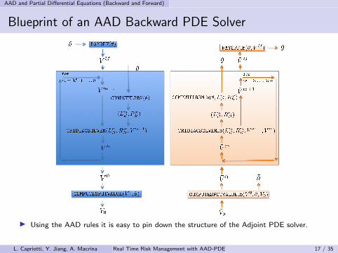
Blueprint of an AAD Backward PDE Solver

I Using the AAD rules it is easy to pin down the structure of the Adjoint PDE solver.



The heart of the algorithm: the tridiagonal solver

I A collection of results on the Adjoint of linear algebra operations (see M. Giles’ ‘CollectedMatrix Derivative Results for Forward and Reverse Mode Algorithmic Differentiation’) isvery useful when dealing with code implementing linear algebra.

I The computational cost of the naıve AAD algorithm above is O(N3). In order to reducethe computational cost to O(N), as in the original algorithm, we need to avoid the matrixinversion by using all the information that is available to us (including the forward sweep!).



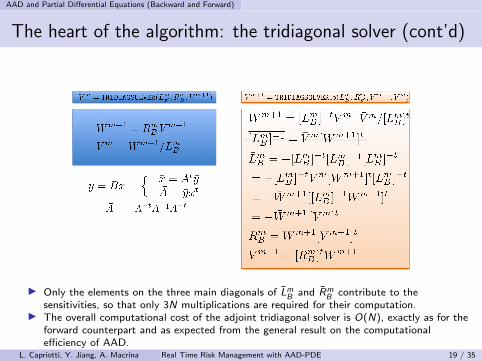
The heart of the algorithm: the tridiagonal solver (cont’d)

I Only the elements on the three main diagonals of LmB and Rm

B contribute to thesensitivities, so that only 3N multiplications are required for their computation.

I The overall computational cost of the adjoint tridiagonal solver is O(N), exactly as for theforward counterpart and as expected from the general result on the computationalefficiency of AAD.



Arrow Debreu Prices and Kolmogorov Forward PDEs

I An approach for derivatives pricing alternative to solving thebackward PDE goes via the Arrow-Debreu (AD) prices, also known asGreen’s functions, defined in this setting as

ψ(y ,T |x , t) = E[δ(y − xT )e−

R Tt ν(xu ,u;θ)du

∣∣∣xt = x],

where δ(·) is the standard Dirac’s delta function.

I AD prices satisfy the following conjugate forward (PDE)

∂tψ(x , t|xt0 , t0)

=(− ν(x , t; θ)− ∂xµ(x , t; θ) +

1

2∂2

xσ2(x , t; θ)

)ψ(x , t|xt0 , t0)

with the initial condition ψ(x , t0|xt0 , t0) = δ(xt0 − x).



Numerical Solution by Finite-Difference Discretization

Forward PDEs can be discretized similarly tobackward PDEs by introducing the vector:

ψm(θ) = (ψ(x1, tm|xt0 , t0), . . . , ψ(xN , tm|xt0 , t0))t

I Starting from a discrete approximation of the AD price at time t0

ψ(x , t0|xt0 , t0) = δ(xt0 − x), on can find the AD prices at time M byiterating a matrix recursion of the form

LF (tm, φ; θ)ψm+1(θ) = RF (tm, φ; θ)ψm(θ)

for m = 0, . . . ,M − 1.



Blueprint of an AAD Forward PDE Solver



Some Results: the Black-Karasinski model for defaultintensities

I To illustrate the efficiency of the AAD-PDE approach theBlack-Karasinki (BK) model for the stochastic instantaneous hazardrate ht = exp xt , namely

d log ht = κ(t)(µ(t)− log ht)dt + σ(t)dWt .

Here, we will fix the mean reversion rate κ = 0.01 and assume µ(t)and σ(t) to be left-continuous piecewise constant functions.

I The conditional probability of the obligor surviving up to time T isgiven by

Q(ht , t,T ) = E[

exp[−∫ T

tdu hu

]∣∣∣ht , τ > t].

I Any credit derivative whose payoff at time T is a function of thehazard rate hT , such as defaultable bonds, CDS, bond options andCDS options can be valued within the PDE approach.



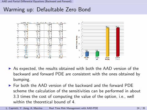
Warming up: Defaultable Zero Bond

I As expected, the results obtained with both the AAD version of thebackward and forward PDE are consistent with the ones obtained bybumping.

I For both the AAD version of the backward and the forward PDEscheme the calculation of the sensitivities can be performed in about3.3 times the cost of computing the value of the option, i.e., wellwithin the theoretical bound of 4.



Bond and CDS Options

I The computational cost of the AAD algorithm is well within thetheoretical bound of 4.

I The overall cost of computing all the sensitivities by means of AAD,relative to the cost of a single valuation of the option, is independenton the number of sensitivities.



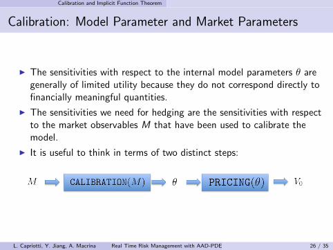
Calibration: Model Parameter and Market Parameters

I The sensitivities with respect to the internal model parameters θ aregenerally of limited utility because they do not correspond directly tofinancially meaningful quantities.

I The sensitivities we need for hedging are the sensitivities with respectto the market observables M that have been used to calibrate themodel.

I It is useful to think in terms of two distinct steps:



Calibration

I As it is customary we have used a combination of the forward andbackward PDE algorithm to bootstrap the survival probabilities andcalibrate to the CDS option prices.



Getting the Market Parameters Sensitivities

I The adjoint of the calibration step M → θ(M) can be producedfollowing the general rules of AAD.

I The computational cost can be expected to be of the order of thecost of performing the calibration algorithm a few (less than 4) times.

I This in itself is generally much better than bumping, involvingrepeating the calibration algorithm as many times as sensitivitiesrequired.

I However, we can do better thanks to ...



Ulisse Dini and the Implicit Function Theorem



Implicit Function Theorem

I The calibration algorithm consists of the numerical solution of asystem of equations of the form

Gi (M, θ) = 0,

with M ∈ RNM , θ ∈ RNθ and i = 1, . . . ,Nθ, where the functionGi (M, θ) is of the form

Gi (M, θ) = Ti (M)− Vi (θ)

where Vi (θ) is the price of the i-th calibration instrument as producedby the model we want to calibrate, and Ti (M) are the prices of thetarget instruments.

I By differentiating with respect to M

∂Gi

∂Mm+

Nθ∑j=1

∂Gi

∂θj

∂θj

∂Mm= 0

for m = 1, . . . ,NM .



Implicit Function Theorem (cont’d)

I Or equivalently

∂θk

∂Mm= −

[(∂G

∂θ

)−1 ∂G

∂M

]km

with [∂G/∂M]ij = ∂Gi/∂Mj .I This relation allows the computation of the sensitivities of θ(M),

locally defined in an implicit fashion by the calibration equation, interms of the sensitivities of the function G . These can be computedby implementing the corresponding adjoint function

(M, θ) = G (M, θ, G )

giving according to the general rule

Mm =

Nθ∑i=1

Gi∂Gi

∂Mmθk =

Nθ∑i=1

Gi∂Gi

∂θk.



Implicit Function Theorem (cont’d)

I The Implicit Function Theorem method is significantly more stableand efficient than of calculating the derivatives of the implicitfunctions M → θ(M) by applying AAD to the calibration step.

I This is because Gi (M, θ) = Ti (M)− Vi (θ) are explicit functions ofthe model and market parameters that are easy to compute anddifferentiate, e.g., using the AAD version of the combination of theforward and backward PDE for the calculation of Vi (θ) and the AADversion of the algorithm for the computation of Ti (M).

I Combining the implicit function theorem with AAD results inextremely efficient risk computations.



AAD and the Implicit Function Theorem: Results

I Combining AAD with the Implicit Function Theorem allows the computation of risk in50% less than the cost of computing the option value, resulting in remarkable savings incomputational time.


Conclusions

Conclusions

I Adjoint Algorithmic Differentiation (AAD) can be used to implementefficiently and in full generality the calculation of sensitivities ofoption prices computed by means of the numerical solution of PartialDifferential Equations (PDE).

I In particular, by combining the adjoint versions of the algorithms forthe numerical solution of a backward and forward PDEs, and theImplicit Function Theorem one can avoid the necessity of repeatingmultiple times the calibration algorithm or implementing the AADversion of the calibration routine.

I This allows the calculation of all price sensitivities for an additionalcomputational cost that is a small multiple of the cost of computingthe P&L of the portfolio, thus typically resulting in orders ofmagnitudes savings in computational time with respect to standardfinite-difference approaches.


Conclusions

References I

[1] L. Capriotti, Fast Greeks by Algorithmic Differentiation, J. of Comp. Finance 14, 3 (2011).

[2] L. Capriotti and M. Giles, Algorithmic Differentiation: Adjoint Greeks Made Easy, RiskMagazine 25, 95 (2012).

[3] L. Capriotti, M. Peacock, and J. Lee, Real Time Counterparty Credit Risk in Monte Carlo,Risk Magazine 24, 86 (2011).

[4] M. Henrard, Calibration and Implicit Function Theorem, OpenGamma QuantitativeResearch, 1 (2011).

[5] L. Capriotti and J. Lee, Adjoint Credit Risk Management, Risk Magazine 27, 90 (2014).

[6] L. Capriotti, Y. Jiang, A. Macrina, Real-Time Risk Management: An AAD-PDE Approach,Int. J. of Fin. Eng. 2, 1550039 (2015).

See also:

My Publications’ Page


http://luca-capriotti.net/publications-finance.html

Real Time Risk Management: An AAD-PDE Approach Capriotti.pdf · Real Time Risk Management: An...

Documents

Transcript of Real Time Risk Management: An AAD-PDE Approach Capriotti.pdf · Real Time Risk Management: An...