Real Time Modeling of Engine Coolant...

Real Time Modeling of Engine CoolantTemperatureIn Engine with Double Cooling Circuits at Two Temperature Levels

Master’s thesis in Innovative and Sustainable Chemical Engineering

CAROLINE PALM

Department of Applied MechanicsCHALMERS UNIVERSITY OF TECHNOLOGY

Gothenburg, Sweden 2017

Master’s thesis 2016:84

Real Time Modeling of Engine Coolant Temperature

In Engine with Double Cooling Circuits at Two Temperature Levels

CAROLINE PALM

Department of Applied MechanicsDivision of Combustion

Chalmers University of TechnologyGothenburg, Sweden 2017

Real Time Modeling of Engine Coolant TemperatureIn Engine with Double Cooling Circuits at Two Temperature LevelsCAROLINE PALM

© CAROLINE PALM, 2017.

Supervisors: André Haury, Volvo CarsOla Waldemarsson, Volvo Cars

Examiner: Sven B Andersson, Applied Mechanics

Master’s Thesis 2016:84ISSN 1652-8557Department of Applied MechanicsDivision of CombustionChalmers University of TechnologySE-412 96 GothenburgTelephone +46 31 772 1000

Cover: Volvo XC90.

Typeset in LATEXPrinted at Applied MechanicsGothenburg, Sweden 2017

iv

Real Time Modeling of Engine Coolant TemperatureIn Engine with Double Cooling Circuits at Two Temperature LevelsCAROLINE PALMDepartment of Applied MechanicsChalmers University of Technology

Abstract

An engine with double cooling circuits operating at two temperature levels has been de-veloped at Volvo Cars. In this thesis the cooling circuit at the lower temperature level isstudied and a model estimating the coolant temperature in this circuit has been developedin Simulink/TargetLink. The model is to be implemented in the engine control unit andused for function based diagnosis of the cooling system.

The cooling system consists of the following components: a water cooled air cooler whichis used to cool the charged air entering the engine, turbochargers in two-stages withcooled bearings systems and a cooled compressor house in one of the turbochargers, aninlet throttle (ETM) cooled for component protection, an SCR injector also cooled forcomponent protection, and a radiator used to cool the coolant. After an investigationof the average heat transfer rate from each component, the ETM was excluded fromthe model. The SCR injector was also excluded since this component had not yet beeninstalled in the studied engine.

The model was formulated with a physical foundation, using energy balances of the systemas well as experimentally obtained heat transfer relationships. An overall energy balancewas used to calculate the coolant temperature in each discrete time step, based on heattransfer from the modeled components in the system (the water cooled air cooler, tur-bochargers and radiator). Model evaluation was performed using vehicle data obtainedfrom real time measurements in a four cylinder diesel engine with extra measurementsensors installed in the air system and cooling system.

The developed model estimates the temperature with a total mean error of −0.2 ◦C. The95 th and 5 th percentile for all simulated data is 1.4 ◦C respectively −2.8 ◦C. The modelwas also shown to be robust against input errors in a sensitivity analysis done for arepresentative test case.

Keywords: engine, cooling system, double cooling circuit, temperature, modeling, watercooled air cooler, turbocharger, radiator, Simulink, diagnosis.

v

Acknowledgements

This thesis work was carried out at Volvo Car Corporation, at the section for Diagnosticsand Dependability. I would like to express my gratitude towards my supervisors AndréHaury and OlaWaldemarsson for their endless support and invaluable feedback throughoutthe project. I would also like to give thanks to group manager Martina Steineck for givingme the opportunity to perform my thesis work at her group and for giving me a warmwelcome. Lastly, thanks to all members of the group for showing me various tips andtricks along the way, and for all well needed coffee breaks.

Caroline Palm, Gothenburg, January 2017

vii

Contents

List of Figures xi

List of Tables xv

1 Introduction 11.1 Background . . . . . . . . . . . . . . . . . . . . . . . . . . . . . . . . . . . . 11.2 Project Description and Aim . . . . . . . . . . . . . . . . . . . . . . . . . . 21.3 Limitations . . . . . . . . . . . . . . . . . . . . . . . . . . . . . . . . . . . . 21.4 Thesis Outline . . . . . . . . . . . . . . . . . . . . . . . . . . . . . . . . . . 3

2 Theory 52.1 Heat Transfer Theory . . . . . . . . . . . . . . . . . . . . . . . . . . . . . . 5

2.1.1 Convection . . . . . . . . . . . . . . . . . . . . . . . . . . . . . . . . 62.1.2 Conduction . . . . . . . . . . . . . . . . . . . . . . . . . . . . . . . . 62.1.3 Radiation . . . . . . . . . . . . . . . . . . . . . . . . . . . . . . . . . 6

2.2 System Description . . . . . . . . . . . . . . . . . . . . . . . . . . . . . . . . 72.2.1 Diesel Engine Air System . . . . . . . . . . . . . . . . . . . . . . . . 82.2.2 Low Temperature Cooling Circuit . . . . . . . . . . . . . . . . . . . 8

2.2.2.1 Radiator . . . . . . . . . . . . . . . . . . . . . . . . . . . . 92.2.2.2 Turbocharger . . . . . . . . . . . . . . . . . . . . . . . . . . 102.2.2.3 Water Cooled Air Cooler and Electronic Throttle Module . 112.2.2.4 SCR injector . . . . . . . . . . . . . . . . . . . . . . . . . . 11

2.3 Engine Control and Diagnostics . . . . . . . . . . . . . . . . . . . . . . . . . 122.3.1 The Engine Control Unit – ECU . . . . . . . . . . . . . . . . . . . . 122.3.2 Fault Diagnosis . . . . . . . . . . . . . . . . . . . . . . . . . . . . . . 12

3 Methods 153.1 Model Formulation in Simulink/TargetLink . . . . . . . . . . . . . . . . . . 153.2 Measurements with INCA . . . . . . . . . . . . . . . . . . . . . . . . . . . . 15

3.2.1 Data Collection . . . . . . . . . . . . . . . . . . . . . . . . . . . . . . 163.3 Model Evaluation and Sensitivity Analysis . . . . . . . . . . . . . . . . . . . 16

4 Model Description 174.1 Main Model . . . . . . . . . . . . . . . . . . . . . . . . . . . . . . . . . . . . 174.2 Radiator Subsystem . . . . . . . . . . . . . . . . . . . . . . . . . . . . . . . 18

4.2.1 Thermostat . . . . . . . . . . . . . . . . . . . . . . . . . . . . . . . . 214.3 Water Cooled Air Cooler Subsystem . . . . . . . . . . . . . . . . . . . . . . 234.4 Turbocharger Subsystem . . . . . . . . . . . . . . . . . . . . . . . . . . . . . 24

4.4.1 Energy Balance Approach . . . . . . . . . . . . . . . . . . . . . . . . 24

ix

Contents

4.4.2 Lookup Table Approach . . . . . . . . . . . . . . . . . . . . . . . . . 254.5 Electronic Throttle Module . . . . . . . . . . . . . . . . . . . . . . . . . . . 274.6 SCR injector . . . . . . . . . . . . . . . . . . . . . . . . . . . . . . . . . . . 274.7 Calibration Procedure . . . . . . . . . . . . . . . . . . . . . . . . . . . . . . 27

5 Results and Discussion 295.1 Cooling Circuit Heat Transfer Estimation . . . . . . . . . . . . . . . . . . . 295.2 Model Evaluation . . . . . . . . . . . . . . . . . . . . . . . . . . . . . . . . . 30

5.2.1 Highway Driving . . . . . . . . . . . . . . . . . . . . . . . . . . . . . 305.2.2 City Driving . . . . . . . . . . . . . . . . . . . . . . . . . . . . . . . 315.2.3 Mixed Driving . . . . . . . . . . . . . . . . . . . . . . . . . . . . . . 325.2.4 Statistical Analysis of the Model Error . . . . . . . . . . . . . . . . . 33

5.3 Sensitivity Analysis . . . . . . . . . . . . . . . . . . . . . . . . . . . . . . . . 355.4 Model Initialization . . . . . . . . . . . . . . . . . . . . . . . . . . . . . . . . 365.5 Calibration of the Model . . . . . . . . . . . . . . . . . . . . . . . . . . . . . 385.6 Possible Model Improvements . . . . . . . . . . . . . . . . . . . . . . . . . . 38

6 Conclusion 41

Bibliography 43

A Installed Extra Sensors I

B Thermostat Model III

x

List of Figures

1.1 Concept of a double cooling circuit. The high temperature circuit ensurescooling of the engine, oil and other high temperature needs. The low tem-perature circuit provides cooling of the charged air, the turbocharger andother low temperature needs. . . . . . . . . . . . . . . . . . . . . . . . . . . 2

2.1 Schematic overview of the air system of the studied diesel engine. The bluelines represent air and the red represent exhaust gas. The orange circlesin the figure are sensors with abbreviations: IAT = intake air temperaturesensor, AMM = air mass meter, MAP = manifold pressure sensor, EMAP= exhaust manifold pressure sensor, EGT = exhaust gas temperature sen-sor, λ-LIN = linear lambda sensor, NOx = nitrogen oxides sensor, DPFdP = differential pressure sensor for diesel particulate filter, EGR dP =differential pressure sensor for exhaust gas recirculation, Soot = soot sensor. 8

2.2 Schematic drawing of the LT coolant circuit. The sensor in the figure mea-sure the temperature which the model is to mimic. ETM is the electronicthrottle module, WCAC is the water cooled air cooler, SCR is the SCRinjector, LP and HP turbo are the low-pressure respectively high-pressureturbochargers. The square is the thermostat. The thick line represents themain coolant flow, the thinner line is a smaller fraction of the flow. . . . . . 9

2.3 Basic principle of engine control. . . . . . . . . . . . . . . . . . . . . . . . . 12

2.4 Model based diagnosis. Input to the system x(t) gives output y(t) and isused to calculate the model output y(t). The residual r(t) is the basis fordiagnosis. . . . . . . . . . . . . . . . . . . . . . . . . . . . . . . . . . . . . . 13

4.1 The main model calculating the coolant temperature from the summarizedheat transfer from cooling of the turbocharger, the water cooled air coolerand the radiator. . . . . . . . . . . . . . . . . . . . . . . . . . . . . . . . . . 18

4.2 Supplier data of radiator heat transfer rate at coolant flow rates rangingfrom 0.1−0.5 kg/s and air flows ranging from 0.25−3.5 kg/s at a temperaturedifference between coolant and air of 45 ◦C. . . . . . . . . . . . . . . . . . . 19

4.3 Heat transfer rate per Kelvin as function of air flow and coolant flow, ob-tained from supplier data in figure 4.2. . . . . . . . . . . . . . . . . . . . . . 19

4.4 Map of the air flow through the radiator at varying vehicle speed and fanspeed. . . . . . . . . . . . . . . . . . . . . . . . . . . . . . . . . . . . . . . . 20

xi

List of Figures

4.5 The radiator subsystem. The resulting heat transfer rate from the radiatoris calculated using supplier characteristics of the radiator in a map withcoolant flow rate (depending on thermostat opening) and air flow rate (asa function of vehicle speed, fan speed and grille shutter position) as input.The heat rate per Kelvin is multiplied with the temperature difference be-tween the ambient air and the coolant temperature at the previous timestep to yield the radiator heat transfer rate. . . . . . . . . . . . . . . . . . . 21

4.6 Schematic view of the radiator with extra temperature sensors Trad,in,Trad,out and TWCAC,in. The square symbolizes the thermostat determin-ing the amount of coolant passing through the radiator. The total coolantflow is denoted mtot, mrad is the mass flow of coolant passing through theradiator and mtot − mrad will bypass the radiator. . . . . . . . . . . . . . . 22

4.7 Calculated thermostat opening against sensor temperature obtained byvarying the sensor temperature during constant acceleration according tothe bottom figure. The red lines are the linear approximation. . . . . . . . . 23

4.8 The WCAC subsystem. The resulting heat transfer rate from the WCAC iscalculated based on air side information in the heat exchanger. Boost tem-perature is the temperature of the air entering the WCAC, inlet manifoldtemperature is the temperature of the air exiting the WCAC (entering theengine cylinders). Throttle flow is modelled within the car software. . . . . 24

4.9 Density plot of calculated heat transfer rate in turbo bearings against theexhaust gas temperature measured after the turbines. . . . . . . . . . . . . 25

4.10 Density plot of calculated heat transfer rate in LP compressor house againstthe air pressure difference across the compressor. . . . . . . . . . . . . . . . 26

4.11 The turbocharger subsystem. A lookup table using the filtered differencein pressure across the LP compressor as input to obtain the compressorhouse heat transfer rate. The heat transfer rate from the turbo bearingsis obtained in a lookup table with the exhaust gas temperature after theturbine as input. . . . . . . . . . . . . . . . . . . . . . . . . . . . . . . . . . 27

5.1 Calculated mean heat transfer rate in each component in the circuit calcu-lated from the installed extra temperature sensors and estimated mass flowrate through the components. . . . . . . . . . . . . . . . . . . . . . . . . . . 30

5.2 Results from simulation of highway driving. Top left: temperature com-parison between actual sensor temperature and the estimated model tem-perature. Bottom left: vehicle speed. Top right: total heat transfer rateto the coolant. Bottom right: heat transfer contribution from each of thecomponents in the model. . . . . . . . . . . . . . . . . . . . . . . . . . . . . 31

5.3 Results from simulation of city driving. Top left: temperature compari-son between actual sensor temperature and the estimated model temper-ature. Bottom left: vehicle speed. Top right: total heat transfer rate tothe coolant. Bottom right: heat transfer contribution from each of thecomponents in the model. . . . . . . . . . . . . . . . . . . . . . . . . . . . . 32

5.4 Results from simulation of mixed driving. Top left: temperature compar-ison between actual sensor temperature and the estimated model temper-ature. Bottom left: vehicle speed. Top right: total heat transfer rate tothe coolant. Bottom right: heat transfer contribution from each of thecomponents in the model. . . . . . . . . . . . . . . . . . . . . . . . . . . . . 33

xii

List of Figures

5.5 Density plot of the model error against time. The black line is the meanerror. The color represents the number of samples (from blue to red) ineach bin. . . . . . . . . . . . . . . . . . . . . . . . . . . . . . . . . . . . . . 34

5.6 Normalized histogram of the model error for all measured data. The greenline marks the mean error. The red line is the median. The blue lines arethe 95 th and 5 th percentile of the error. . . . . . . . . . . . . . . . . . . . . 34

5.7 Density plot of the model error against boost pressure. The color representsthe number of samples (from blue to red) in each bin. . . . . . . . . . . . . 35

5.8 Resulting mean error increase from multiplying each parameter with a fac-tor of 0.8, 1.2 and 1.5. Based on the mixed driving measurement in section5.2.3. . . . . . . . . . . . . . . . . . . . . . . . . . . . . . . . . . . . . . . . . 36

5.9 The effect of initialization shown for the mixed driving case in section 5.2.3. 37

B.1 Thermostat model. . . . . . . . . . . . . . . . . . . . . . . . . . . . . . . . . III

xiii

List of Figures

xiv

List of Tables

4.1 Compensation factor multiplied with the radiator air flow rate at differentgrille shutter positions. 0 % is when the grille is completely shut and 100 %is when the grille is completely open. . . . . . . . . . . . . . . . . . . . . . . 20

5.1 Resulting model error for highway driving, calculated as the difference be-tween the measured sensor temperature and the estimated temperature. . . 31

5.2 Resulting model error for city driving, calculated as the difference betweenthe measured sensor temperature and the estimated temperature. . . . . . . 32

5.3 Resulting model error for mixed driving, calculated as the difference be-tween the measured sensor temperature and the estimated temperature. . . 33

A.1 Relevant extra measurement sensors installed in the test vehicle. . . . . . . I

xv

List of Tables

xvi

1Introduction

As a way of reducing environmental issues related to the transport sector the emissionlegislation is becoming more stringent. This pushes technical innovation in the vehicleindustry to meet these requirements without compromising good engine performance (suchas torque and acceleration). In a step towards meeting future demands Volvo Cars hasdeveloped an engine platform where one of the changes include the introduction of a secondcooling circuit.

1.1 Background

In several parts of the world emissions from internal combustion engines are regulatedby legislation. Regulated emissions include hydrocarbons (HC), carbon monoxide (CO),nitrogen oxides (NOx) and particulates, the emission limits and conditions are regularlyupdated [1]. In the European Union emissions are regulated by so called Euro emissionstandards and the current standard for light duty vehicles is Euro 6 [2]. As mentionedpreviously the emission requirements are continuously updated, and one upcoming change(phase-in starting September 2017) is that all emission tests are to be done under real driv-ing conditions with a so called Real Driving Emissions test procedure (RDE) as apposed toprevious laboratory testing [1, 2]. EU legislation has also introduced mandatory emissionreduction targets for carbon dioxide (CO2) of 130 g CO2/km from 2015 and 95 g CO2/kmby 2021, which is directly related to fuel consumption [3, 4, 5]. These kinds of changes inlegislation acts as a driving force that pushes and encourages technical solutions regard-ing internal combustion engines, with lower emissions at unchanged or increased engineperformance.

Is has been shown that the engine cooling system has large influence on the emissions andthat an optimized cooling system can, at a relatively low cost, yield a decrease in bothprimary pollutants and CO2 [4, 5, 6]. One strategy to improve the cooling system perfor-mance is to divide the cooling system into two separate circuits at different temperaturelevels, with benefits such as reduced fuel-consumption, improved engine warm-up and im-proved air boosting [4, 5, 7]. This type of system can be illustrated as in figure 1.1 wherea high temperature radiator provides cooling of the engine and other high temperatureneeds and the circuit operating at lower temperature ensures cooling of components withlower temperature needs. This strategy has been incorporated into Volvo Cars engineplatform.

The above mentioned emission requirements should not only be fulfilled when the car isnew. There is also legislation regarding detecting faults occurring in the car that canincrease emissions, throughout the lifetime of the car – On-Board Diagnostics (OBD)

1

1. Introduction

High Temperature Radiator

Low Temperature Radiator

Low Temperature Needs

High Temperature Needs

Figure 1.1: Concept of a double cooling circuit. The high temperature circuit ensures cooling ofthe engine, oil and other high temperature needs. The low temperature circuit provides cooling ofthe charged air, the turbocharger and other low temperature needs. Figure redrawn from [5].

regulations [1, 8]. Basically this legislation says that the driver must be notified if a faultor malfunction occurs that causes emissions to increase over some threshold values [1].Diagnostic functions are therefore implemented into the engine control unit (ECU) anddecide whether there is a fault in the system or not, and identify the fault. One diagnosticmethod is model based diagnosis, where faults are detected by comparing a measuredsensor value to a predicted (modeled) value [8].

Regarding the coolant system, faults that can affect emissions are thermostat faults (leak-ing etc.) and sensor faults. These kinds of faults can be detected by using a model. Andfor Volvo Cars double circuit coolant system a model for the high temperature circuit isalready available in the ECU, but a model for the low temperature circuit needs to beimplemented.

1.2 Project Description and Aim

The aim of the thesis work is to develop a model in Simulink/TargetLink that estimates thecoolant temperature in the low temperature cooling circuit. The temperature estimationshould have a physical foundation and use information available in the ECU. The modelshould be composed in such a way that it can easily be modified to handle different setupsof hardware that could be connected to the circuit. Ease of calibration for different car orengine variants should also be considered.

Model validation is to be done in Simulink using real world vehicle data obtained fromtesting in a vehicle equipped with extra measurement sensors. The finished model shouldthen be able to be implemented into the ECU.

1.3 Limitations

The model is developed for a four cylinder diesel engine. Although the model should havethe possibility to be modified for other engine variants and different hardware setups, it isoutside the scope of the thesis to do so and only the diesel engine will be considered.

The method for model initialisation is not considered in this thesis. Instead the tempera-ture sensor in the coolant circuit is used to initialize the model.

2

1. Introduction

Due to the early stage of the engine development project, the engine control systems arenot yet completely calibrated. For instance the control of the coolant flow in the circuit hasnot yet been calibrated and therefore the coolant flow is at its maximum level throughoutthe project. All validation measurements are made at maximum fan speed and completelyopen grille shutter, although these parameters are varied to find the radiator air flow rate.Once the control system is complete the model might need slight adjustments.

1.4 Thesis Outline

The thesis report is divided into six chapters. This introduction is followed by chapter2, containing general theory of heat transfer, a description of the studied system and anintroduction to engine control and diagnosis.

In chapter 3 the method used for developing the model is described. This includesthe model development in Simulink/TargetLink, measurements in car and model vali-dation.

The developed model is described in chapter 4. This chapter starts with an overview ofthe model, before going into detail about each subsystem in the model.

For the final model, the results is presented and discussed in chapter 5. The resultscontain a comparison of the estimated temperature and the actual sensor temperature inthe circuit. This is then concluded in chapter 6.

3

1. Introduction

4

2Theory

The physical basis for describing the temperature change of the coolant is heat transferfrom the components in the system. In this chapter basic heat transfer theory will be given,followed by a description of the studied system. At the end of the chapter, engine controland diagnosis will be introduced to give an overview of the intended model application –function based diagnosis.

2.1 Heat Transfer Theory

One of the fundamental laws of physics is the first law of thermodynamics. This law isbased on conservation of energy, that energy can neither be created nor destroyed, andstates that

If a system is carried through a cycle, the total heat added to the system fromits surroundings is proportional to the work done by the system on its sur-roundings. [9]

For a system with a certain control volume the first law of thermodynamics can, accordingto [9], be expressed as

rate of additionof heat to con-trol volume fromits surroundings

−

rate of work doneby control volumeon its surround-ings

=

rate of energy outof control volumedue to fluid flow

−

rate of energyinto control vol-ume due to fluidflow

+

rate of accumu-lation of energywithin controlvolume

.

(2.1)

This is the general energy balance for the system.

A device with primary purpose of transferring energy from a hot fluid to a cold fluid isknown as a heat exchanger [9]. The basis for any heat exchanger is conservation of energyand the energy balance can be written for the individual streams in the heat exchanger,or the system boundaries can be defined around the entire heat exchanger. Defining thesystem boundaries around the entire heat exchanger, assuming no heat loss (adiabatic),

5

2. Theory

the energy in the inlets must be equal to the energy in the outlets. This means that allenergy lost in the hot fluid will be gained by the cold [10]. Defining Q as the rate of heattransfer from the hot fluid, this can be expressed as

Q = (mCP )h(Th,in − Th,out) = (mCP )c(Tc,out − Tc,in), (2.2)

where m is the mass flow rate of the fluid, CP is the heat capacity of the fluid and Tinand Tout is the temperature in respectively out of the heat exchanger. The index h and cdenotes the hot respectively cold stream.

Heat transfer is usually divided into three different heat transfer mechanisms: convection,conduction and radiation. These types of heat transfer is explained further in the followingsections.

2.1.1 Convection

The heat transfer between a surface and an adjacent fluid is categorized as convective heattransfer [9]. The rate for convection is expressed by the Newton rate equation:

Q

A= h∆T, (2.3)

where Q is the rate of convective heat transfer, A is the surface area normal to the directionof the heat flow, ∆T is the difference in temperature between the surface and the fluidand h is the convective heat transfer coefficient [9]. Important parameters determiningthe heat transfer rate for convective heat transfer are the magnitude of the temperaturedifference (∆T ), the geometry of the system and properties of the fluid and the fluid flow[9].

2.1.2 Conduction

Heat transfer by conduction is primarily a molecular phenomenon, where the motion ofa molecule at a higher energy level imparts energy to adjacent molecules at lower energylevels [9]. Fourier’s first law of heat conduction for heat transfer in x-direction describesthe heat transfer rate as

QxA

= −kdTdx, (2.4)

where Qx is the conductive heat transfer rate, A is the area normal to the heat flowdirection, dT

dx is the temperature gradient in the x-direction and k is the conductivitywhich is a material specific property [9].

2.1.3 Radiation

Heat transfer by radiation is different from convection and conduction in that no mediumis needed to transfer the heat [9].

6

2. Theory

For a perfect radiator (a black body that does not reflect nor transmit any thermal radi-ation) the thermal rate equation is used to describe the heat transfer rate:

Q

A= σT 4 = Eb, (2.5)

this equation is also known as the Stefan-Boltzmann equation [9]. Eb = QA is the heat

transfer rate per area of the emitting surface also known as the total emissive power of ablack body, σ is the Stefan-Boltzmann constant and T is the surface temperature.

For actual surfaces the total emissive power will be less than that for a black body, sincesome thermal radiation will be reflected and transmitted. This is described with theemissivity, ε, defined as the ratio between the total emissive power of the surface and thetotal emissive power of a black body at the same temperature (ε = E

Eb) [9].

The net rate of radiant energy transfer between two objects (1 and 2) at different temper-ature can be expressed as

Q1,2 = σA1F1,2(T 41 − T 4

2 ), (2.6)

where F1,2 is a function of the shape factors and emissivity of both objects [11]. Fora configuration where one object (1) is completely surrounded by the other object (2)equation (2.6) can be written as

Q1,2 = σ(T 41 − T 4

2 )1

ε1A1+ 1−ε2

ε2A2

. (2.7)

And when the enclosure is much larger than the enclosed object (A2 � A1), as for anobject in a large, isothermal environment at temperature T2 = T∞, the expression can besimplified to

Q1,2 = εσA1(T 41 − T 4

∞), (2.8)

which is useful for describing the heat transfer when a hot object is radiating to its envi-ronment [11].

2.2 System Description

The system studied is, as mentioned in section 1.3, a four cylinder diesel engine equippedwith double cooling circuits. The cooling circuits differs slightly between different enginevariants depending on if it is a diesel or a petrol engine, the engines can also have slightlydifferent hardware configurations (e.g. one-stage or two-stage turbocharging). However, inthis section only the diesel engine studied is described. First the air system for the engineis introduced, then the low temperature cooling circuit and its included components isdescribed.

7

2. Theory

2.2.1 Diesel Engine Air System

The air system for the studied engine is shown in figure 2.1. Ambient air enters through thefront grille and spoilers of the vehicle and passes heat exchangers placed at the front. Theintake air then pass through an air filter that removes impurities. The air is compressedfor improved efficiency in turbochargers in two stages. Compressing the air raises itstemperature, and therefore the charged air passes a heat exchanger (charge air cooler)before reaching the engine inlet manifold. The air then enters the engine cylinders, fuel isinjected and the combustion process takes place. The exhaust from the combustion passesthrough the turbine side of the two turbochargers before it reaches the aftertreatmentsystem consisting of a combination of a lean NOx trap (LNT) and selective catalyticreduction with a diesel particulate filter (SCRF). The exhaust gases are then emitted tothe ambient via the exhaust pipe.

Figure 2.1: Schematic overview of the air system of the studied diesel engine. The blue linesrepresent air and the red represent exhaust gas. The orange circles in the figure are sensors withabbreviations: IAT = intake air temperature sensor, AMM = air mass meter, MAP = manifoldpressure sensor, EMAP = exhaust manifold pressure sensor, EGT = exhaust gas temperaturesensor, λ-LIN = linear lambda sensor, NOx = nitrogen oxides sensor, DPF dP = differentialpressure sensor for diesel particulate filter, EGR dP = differential pressure sensor for exhaust gasrecirculation, Soot = soot sensor.

2.2.2 Low Temperature Cooling Circuit

As described in the introduction, the cooling of the engine system is divided into twocircuits. One operating at a high temperature level, and one at a lower temperature levelfor cooling at lower temperature needs. The low temperature circuit (LT-circuit), whichis the focus of this thesis, is responsible for cooling the charged air in the heat exchanger

8

2. Theory

located before the inlet manifold, the turbochargers, the electronic throttle module at theinlet manifold (Throttle A in figure 2.1), and the SCR injector. A schematic drawingof the low temperature cooling system is shown in figure 2.2. The sensor in the figure,located before the thermostat (square), is the temperature sensor which the model is tomimic. The coolant flow is divided after the pump, where the main flow (thicker line) goesthrough the WCAC (water cooled air cooler) and the rest is divided between the ETM,SCR injector and turbocharger bearings. The LP turbocharger is cooled by two coolantstreams: one cooling the turbocharger bearings and one cooling the compressor house inthe turbocharger (further explained in 2.2.2.2). The thermostat regulates if the flow ispassing through the radiator, or is bypassed (see section 2.2.2.1).

Rad

iato

r

ETM WCAC SCR

LP Turbo HP TurboSensor

Figure 2.2: Schematic drawing of the LT coolant circuit. The sensor in the figure measurethe temperature which the model is to mimic. ETM is the electronic throttle module, WCACis the water cooled air cooler, SCR is the SCR injector, LP and HP turbo are the low-pressurerespectively high-pressure turbochargers. The square is the thermostat. The thick line representsthe main coolant flow, the thinner line is a smaller fraction of the flow.

Usually coolant is an aqueous solution of ethylene glycol (50 vol-%) [12]. In contrast tothe HT-circuit which uses a pump driven by the engine crank, an electrical pump is usedto pump the coolant in the LT-circuit. This makes it possible to circulate coolant in thesystem even after the engine had been shut off (known as after run), which can be usedfor component protection.

The components in the LT-circuit is explained in further detail below with focus on theoccurring heat transfer.

2.2.2.1 Radiator

As the coolant flow through the components in the LT-circuit it will accumulate heatbefore it reaches the radiator where the coolant is cooled itself. The radiator is a type ofheat exchanger located in the front of the vehicle (behind the grille) utilizing ambient airto cool the coolant flowing through its finned heat exchanger tubes [12].

The heat transfer between the coolant and air occurs by conduction through the tube wallsand fins as well as by convection [12]. As with all heat transfer, the temperature differencebetween the coolant and the air is an important aspect determining the heat transfer ratein the radiator. Two other important aspects of the radiator cooling power is coolant flowand air flow, which in contrast to the temperature difference can be controlled.

9

2. Theory

In order to avoid overcooling of the coolant, keeping the coolant temperature optimal,the coolant flow is sometimes directed past the radiator [13]. This is controlled by a self-regulating wax thermostat which opening area is determined by the temperature of thecoolant.

Generally the air flow through the radiator is determined by the vehicle speed. However,the air flow can be controlled by using radiator shutters (grille shutter and spoiler shutter)and a radiator fan. The radiator shutters are vanes that blocks air flow through the grilleand spoilers, this is done both in order to control the temperature of the coolant butalso to reduce drag (improve fuel economy) [13]. The radiator fan is placed behind theheat exchangers to regulate the air flow, this is particularly useful when idling since the"natural" air flow caused by driving then is close to zero.

2.2.2.2 Turbocharger

The air supply to the combustion chamber is an important aspect in engine control, sincethe air supply impacts engine performance as well as the emissions and fuel consumption[14]. One way to optimize the air supply is by using a turbocharger. A turbochargerutilize the hot exhaust gas flow in a turbine to generate power used to compress the intakeair in a compressor directly coupled to the turbine by a shaft [15].

The process of compressing the intake air in order to supply the engine with more air isreferred to as boosting, supercharging or pressure charging. The compression increase thedensity of the air, and hence the mass of air in the engine cylinder, which means thata proportional extra amount of fuel can be added yielding an increased power output orthus allows engine downsizing [14]. The turbocharger can be considered a form of wasteheat recovery, since it utilizes the otherwise unused thermal energy in the exhaust gas andimprove the efficiency of the engine [14].

The engine studied in the thesis has controlled two-stage turbocharging with two tur-bochargers in series with a controlled bypass on the compressor side (HPC bypass infigure 2.1) [16]. The first turbocharger (seen from the inlet air point of view in figure2.1), the so called low-pressure (LP) turbocharger, is larger than the second, so calledhigh-pressure (HP) turbocharger. At low engine speeds the HPC bypass valve is closedand the high-pressure turbocharger is used, resulting in rapid development of turbochargerpressure. Whereas at high engine speeds the bypass valve opens so that only the largerlow-pressure turbocharger is operating.

The turbocharger is also controlled on the turbine side to prevent the turbocharger frombeing damaged or overloading the engine at high exhaust gas flows. This is achieved intwo ways: with a wastegate valve which diverts the flow past the high-pressure turbine athigh engine speeds, and with the turbines having a adjustable geometry (VNT, variablenozzle turbine) that controls the flow rate through the turbines [16, 17]. The VNT isalso used to control the air compression. At low engine speeds, when the high-pressureturbocharger is used, the VNT of the LP turbocharger is closed, hence the LP compressoris not operating.

Exhaust gases from a diesel engine can reach temperatures up to 700−900 ◦C and hence theturbocharger turbine is made of materials that can sustain such high temperatures [18, 19].On the compressor side of the turbocharger temperatures are lower, ranging from 30 −150 ◦C [19]. This large temperature gradient across the turbocharger will yield a significant

10

2. Theory

conduction heat transfer through the less heat tolerant bearing system supporting the shaftconnecting the turbine to the compressor. This heat transfer through the bearings systemmay be problematic and is called heat soak-back [20]. While the engine is running oillubricating the turbocharger shaft will absorb most of this energy thus preventing damageto the turbocharger bearings system. But once the engine is shut off the oil flow stopseven though the bearings still needs cooling. Therefore water cooling of the turbochargerbearings has been introduced, since water can be pumped also after engine shut off by theelectrical pump (after run) [20].

Both turbochargers in the system has cooled bearings systems, seen as the thinner linesthrough the turbochargers in figure 2.2. In the figure it can be seen that the low-pressureturbocharger also is cooled, by the major part of the coolant flow (thick line in the figure).This is to cool the LP turbocharger compressor house.

2.2.2.3 Water Cooled Air Cooler and Electronic Throttle Module

As mentioned above, turbocharging is a way of increasing the density of the intake air.However, the compression also increase the temperature of the air. And since density iscoupled to the temperature (hot air is less dense than cool) a reduction in temperaturecan further increase the density of the charged air, hence more air can be supplied to theengine without increasing the pressure further [16, 21]. Too high temperatures can alsocause too high combustion temperatures, which can affect power, torque and emissions[21]. Therefore, cooling of the charged air is desired.

A common way of achieving the charge air cooling is by using a heat exchanger usuallyreferred to as a charge air cooler (CAC) [21]. Charge air coolers can either utilize air ascooling media (ACAC) or water coolant (WCAC), the latter being introduced in the engineplatform studied in this thesis. Compared to the previously used ACAC, a WCAC hasseveral advantages including smaller pressure drop in the charge air system and improvedtransient response since the WCAC can be placed in direct vicinity to the intake manifoldwhereas a ACAC needs to be located by the radiator and hence giving a longer air path[21, 22]. Since water has a higher heat capacity than air a smaller heat exchanger can beused for a WCAC than a ACAC, thus resulting in weight benefits [21, 22].

In direct vicinity to the WCAC is the electronic inlet throttle (electronic throttle module,ETM) a component that control the flow of air into the engine. To avoid overheating anddamage to this component, it is cooled by coolant in the LT-circuit.

2.2.2.4 SCR injector

In diesel engines the most troublesome emissions are nitrogen oxides (NOx) and partic-ulates [23]. And as a measure towards reducing these emissions due to the regulationsdiscussed in section 1.1 advanced aftertreatment methods are being implemented. In thestudied engine the exhaust aftertreatment system includes a lean NOx trap (LNT) andselective catalytic reduction (SCR) with an integrated diesel particulate filter (SCRF) (seefigure 2.1).

In selective catalytic reduction of NOx urea is injected to the exhaust mixture and decom-pose to ammonia which then reduce the NOx to nitrogen gas N2 [24]. Due to the highexhaust gas temperature (especially after LNT regeneration) the urea injector can be-

11

2. Theory

come overheated. The injected urea cools the injector to some extent but not sufficiently,therefore the injector is cooled by water coolant in the LT-circuit.

2.3 Engine Control and Diagnostics

The finished model will be implemented in the software in the engine control unit (ECU).It will be used by diagnostic functions to detect faults in the low temperature coolingcircuit. A brief introduction to the subject of diagnostics and the basic principle of theECU will be given here.

2.3.1 The Engine Control Unit – ECU

Engine control is the core for over seeing and managing various engine functions [25].The engine control system consists of the engine control unit (ECU), sensors, actuatorsand a communication system. And what was previously controlled mechanically has, astechnology has evolved, transitioned to computerized control by the engine control unit[26].

The ECU consists of electronic components on a microcontroller chip (CPU), a memoryto store information and software [26]. The ECU basically works in the same way as aconventional PC, where data is entered and used to calculate output signals [16].

In the ECU the entered data comes from sensors that measure physical quantities andconverts it to an electric signal proportional to the measured value. The electric signal isprocessed in real-time in the microprocessor of the ECU and instructions to actuators iscalculated. The calculations can be based on mathematical functions or using a set of pre-calculated results covering different engine operating conditions (maps or look-up tables).The calculated instructions are then sent to the actuators controlling different parts of theengine [26]. The basic principle of the engine control with the ECU is illustrated in figure2.3.

SensorsEngineControlUnit

Actuators Engine

Figure 2.3: Basic principle of engine control.

2.3.2 Fault Diagnosis

As mentioned in section 1.1 there is legislation regarding supervision of components andfunctions that cause increased emissions if malfunctioning – the OBD regulations. Thissupervision is known as diagnosis and the diagnostic functions are part of the ECU softwareand detects and identify faults and generate fault codes stored in the ECU memory [8]. Ifa fault is detected an indication to the driver can be sent from the ECU and the generatedfault code is stored and can later be read with specific diagnostic tools, facilitating repairof the car.

One useful method for diagnosis, the method related to this thesis, is model based diagnosis.

12

2. Theory

In model based diagnosis (schematically shown in figure 2.4) a model is formulated basedon known inputs and the output from the model is then compared to the actual systemoutput. Based on the residual between the system and model output a fault decisionis made [8]. Model based diagnosis has the advantages of being a cost-effective methodwith high diagnosis performance (small faults can be detected and the detection time isrelatively short) [8].

System

Modely(t)

−

y(t)x(t)

r(t)

Figure 2.4: Model based diagnosis. Input to the system x(t) gives output y(t) and is used tocalculate the model output y(t). The residual r(t) is the basis for diagnosis. Redrawn from [8].

The model developed in this thesis will be used to detect faults on the temperature sensormeasuring the temperature of the coolant in the circuit. One fault that can occur on thetemperature sensor is a so called ”stuck fault” meaning that the sensor returns the samevalue regardless of the actual state of the system. By comparing the modeled temperatureto the measured sensor value and evaluating the error this type of fault can be found,according to the above described approach.

This approach can also be used if the thermostat is leaking. If the thermostat is stuck openthe coolant temperature sensor will show a lower value than it should at those conditions,since more coolant is passed through the radiator. This is also detected by evaluating theaccumulated error between the model and the sensor temperature.

Once a faulty coolant temperature sensor has been detected the model can further be usedas a replacement value for the sensor, basing the requests to actuators on the modeledtemperature instead of the sensor temperature. This way control functions that dependson the coolant temperature, e.g. coolant pump request, can still function properly.

13

2. Theory

14

3Methods

The project procedure consists of three main parts: model formulation, data gatheringand model evaluation. The model is constructed in Simulink/TargetLink and throughoutthe model development measurements in car are performed and used as input to the modeland for model evaluation. To investigate the influence of uncertainties in the model inputsa sensitivity analysis is performed on the final model.

3.1 Model Formulation in Simulink/TargetLink

The model is formulated in Simulink 2011b with the dSpace TargetLink application.Simulink is a MathWorks block diagram simulation environment where the blocks performmathematical operations on the system input [27]. TargetLink is a software integrated toSimulink that is used to be able to produce C-code directly from the Simulink model.TargetLink has a specific, extended blockset, with all necessary information needed forC-code generation [28]. The TargetLink blockset is used in the model.

The model is formulated in discrete time, with sampled input data from sensors (tem-perature, pressure etc.), actuator requests and modeled values in the ECU software. Thesample time used in the model is 0.08 s.

3.2 Measurements with INCA

All input values to the model are obtained using measured data in real driving conditions.The model can then easily be evaluated by comparing the measured sensor temperatureduring driving with the estimated temperature at those conditions.

To record data from the ECU, engine and additional hardware (installed extra temperatureand flow sensors) while driving the software INCA from ETAS Group is used. INCA isa measurement, calibration and diagnostics tool for automotive electronic systems [29].INCA connects to an ETK (emulator test probe) which in turn is connected in parallelto the ECU, that way all data in the control unit memory is directly accessed [29]. INCAis also connected via CAN bus to access the data from the additional hardware installed(temperature and flow sensors).

In the INCA software, an experiment is created which defines all the relevant signals tobe measured and recorded during driving. These recordings are then used as input to theSimulink model.

15

3. Methods

3.2.1 Data Collection

All measurements are performed in a Volvo XC90 with a four cylinder diesel engineequipped with the double circuit cooling system. In addition to the standard measurementsensors in the car, the test car is equipped with additional measurement sensors to simplifythe model evaluation. The location of relevant extra measurement sensors installed arelisted in appendix A.

The data is gathered for various driving conditions, and is used both to evaluate themodel and also to gain a better understanding of how different driving conditions affectthe cooling system and the model. Examples of different driving conditions are: steadystate driving at constant speed, city driving, highway driving and mixed driving at varyingvehicle speeds. The ambient temperature and other outer conditions vary between the testsand no standardized test cycles are tested.

3.3 Model Evaluation and Sensitivity Analysis

Using the obtained data from measuring in car, the model is continuously validated toimprove and calibrate the model. The extra measurement sensors is used to decomposethe validation further, evaluating each subsystem in the model and not just the finaltemperature. The extra sensors are also used to calibrate the model and find parametersand heat transfer properties.

For the final evaluation of the model the difference between the measured temperature andthe estimated temperature is calculated for a number of different driving cases. For eachcase the maximum difference is also calculated. Using a data evaluation tool in MATLABdeveloped at Volvo Cars a statistical evaluation is performed on a large selection of datagathered through out the project (in total data from 7 hours of driving). The evaluationconsists of a density plot showing the model error as a function of time for all data samples.It also consists of a histogram showing the model error normalized for all data points. Themean error, the median of the error and the 95 th and 5 th percentile of the error are alsocalculated and displayed in the histogram.

A sensitivity analysis of the model is performed for a representative test case, using aone-at-a-time approach [30]. In this approach one parameter value in the model is moved,keeping the others at their baseline values for that measurement. While doing this oneparameter at a time the changes in the output is monitored and the resulting increase in themodel error is calculated. This is then summarized in a bar diagram to give an indicationof faults in the model or in the system that may yield large secondary errors.

16

4Model Description

The model is constructed with one main model, calculating the temperature of the coolanteach discrete time step. The calculations in the main model is based on heat transfer fromthe components in the circuit, modeled in subsystems.

Each part of the model has a physical foundation and the principles and equations usedto develop the model is described is this chapter. First the main model will be describedfollowed by each subsystem in the model.

The resulting Simulink models are shown in each section. For information about the blocksused in the model and the mathematical operations they perform, the reader is referredto Simulink documentation [31].

4.1 Main Model

The general energy balance in (2.1) can, with the coolant as control volume, be simplifiedaccording to

rate of additionof heat to con-trol volume fromits surroundings

=

rate of accumu-lation of energywithin controlvolume

, (4.1)

since the coolant system is a closed system with no heat flows in or out of the system,and the coolant performs no work. This means that all heat added to the coolant controlvolume must be accumulated. Equation 4.1 can be written, and discretized, as

∑Qi = d(ρV CPT )

dt= ρV CP

∆Tts, (4.2)

where∑Qi is the total rate of heat addition to the coolant from each of the components

in the circuit. ρV is the mass of coolant that the heat is transferred to, if the thermostatis closed the coolant mass in the radiator is not included. CP is the heat capacity of thecoolant, obtained from tabulated values in [32]. The temperature difference of the coolantin one time step (ts) is denoted ∆T .

In the main model all heat transfer contributions from the components are summarizedfor each sample and by feeding back the coolant temperature from the previous time step

17

4. Model Description

the current temperature can be calculated using (4.2). The main model is shown in figure4.1 below. To the left in the figure is all input signals to the model, available in the ECUsoftware. The model inputs enters the subsystems where the heat transfer rates in thecomponents are calculated. The mass of coolant in the system depends on whether thethermostat is open or not, if the thermostat is closed the coolant mass in the radiator is notaccounted for. In the first time step the model needs to be initialized, this is currently donewith a switch using the sensor value (seen in the top right of the figure). The initializationwill be further discussed in section 5.4.

Q = m Cp ΔT/ts

ΔT1

tsts

WCAC

z1

Turbo

~=

Radiator

-C-

-C-

Switch

Properties

>=

0

12

1110987

6

5

4

3

2

1

0

Q Coolant

Coolant Heat Capacity

Total Mass of Coolant in System

Q Turbo

Q WCAC

Q RadiatorAmbient TemperatureVehicle SpeedGrille Shutter PositionRequested Fan PWM

Throttle Flow (modelled)

Inlet Manifold Temperature

Boost Temperature

Turbine Outlet TemperatureSensor Temperature

Sample Time

Coolant Density

Thermostat Opening

Mass in Radiator

Mass in Pipes

Requested Coolant Flow

Atmospheric Pressure

Boost Pressure LP Turbo

Estimated Temperature

Figure 4.1: The main model calculating the coolant temperature from the summarized heattransfer from cooling of the turbocharger, the water cooled air cooler and the radiator.

The heat transfer contributions from each component is calculated in subsystems in theglobal Simulink model, in the following sections each of the subsystems in figure 4.1 willbe described.

4.2 Radiator Subsystem

The supplier of the radiator provides data for the heat transfer performance of the radiatorat different air and coolant flow rates measured at a constant temperature difference(45 ◦C) between the coolant and the air. This data is presented in figure 4.2.

18


0 0.1 0.2 0.3 0.4 0.5

Coolant Flow Rate [kg/s]

0

0.5

1

1.5

2

2.5

3

3.5

4

4.5

5

HeatTransfer

Rate

[W]

×104 Heat Performance at 45 ◦C Difference

0.25 kg/s0.5 kg/s1 kg/s1.5 kg/s2 kg/s2.5 kg/s3 kg/s3.5 kg/s

Air Flow Rate

Figure 4.2: Supplier data of radiator heat transfer rate at coolant flow rates ranging from 0.1 −0.5 kg/s and air flows ranging from 0.25−3.5 kg/s at a temperature difference between coolant andair of 45 ◦C.

A linear relationship between the heat rate and the temperature difference is assumed andall data points in figure 4.2 are divided by the temperature difference to obtain a heattransfer rate expressed per unit Kelvin difference in temperature between the coolant andthe ambient air, shown in figure 4.3.

0

200

3

400

0.5

600

HeatTransfer

Rate

[W/K]

800

0.42

Air Flow [kg/s]

1000

0.3

Coolant Flow [kg/s]

1200

0.210.1

0 0

Figure 4.3: Heat transfer rate per Kelvin as function of air flow and coolant flow, obtained fromsupplier data in figure 4.2.

By knowing the coolant temperature calculated in the model (the previous time step) andthe ambient temperature of the air flowing through the radiator the map in figure 4.3 canbe used to model the heat transfer in the radiator. Before the heat transfer rate can beobtained, the flow rate of coolant and air through the radiator is needed.

As mentioned in section 2.2.2.1 the air flow through the radiator is dependent on thevehicle speed, the speed of the fan and the grille shutter position. Based on steady statemeasurements at velocities ranging from 0 − 200 km/h at varying fan speed and grille

19


0

0.5

80200

1

Air

Flow

Rate

[kg/s]

60 150

1.5

Fan Speed [%] Vehicle Speed [km/h]

2

40 1005020

0

Figure 4.4: Map of the air flow through the radiator at varying vehicle speed and fan speed.

shutter positions the air flow through the radiator is estimated with help of the extrasensors installed. To avoid the complexity of having a map with three inputs (a map in 4dimensions) one map is constructed for the vehicle speed and fan speed (seen in figure 4.4),and the grille shutter position is used to obtain a compensation factor, tabulated in table4.1. Linear interpolation between the tabulated values are performed in the model.

Table 4.1: Compensation factor multiplied with the radiator air flow rate at different grille shutterpositions. 0 % is when the grille is completely shut and 100 % is when the grille is completely open.

Grille CompensationGrille Shutter Factor0 % 0.450 % 0.9100 % 1

In the control unit there is a signal for the total coolant flow request sent to the coolantpump. The requested coolant flow rate is converted from l/min to kg/s using the coolantdensity (obtained from tabulated values in [32]), and transformed into actual coolant flowrate using a look-up table with corresponding measured flow rates. However, as mentionedin section 2.2.2.1 coolant is sometimes bypassed the radiator and hence the total coolantflow can not always be used as a whole, the thermostat opening must also be taken intoaccount. This is done by multiplying the total coolant flow rate by the thermostat openingfactor, explained further in the following section (4.2.1).

The final radiator model is presented in figure 4.5.

20


l/min to kg/s

1

Thermostat Opening

rc

Radiator Heat Transfer

Grille Compensation

Coolant Flow60

1000

rc

Air Flow

6

5

4

3

2

1

Coolant Flow through Radiator

Estimated Temperature

Vehicle Speed

Grille Shutter Position

Requested Fan PWM

Ambient Temperature

Heat Rate per Kelvin

Q Radiator

Air Flow through Radiator

Requested Coolant Flow

Figure 4.5: The radiator subsystem. The resulting heat transfer rate from the radiator is calcu-lated using supplier characteristics of the radiator in a map with coolant flow rate (depending onthermostat opening) and air flow rate (as a function of vehicle speed, fan speed and grille shutterposition) as input. The heat rate per Kelvin is multiplied with the temperature difference betweenthe ambient air and the coolant temperature at the previous time step to yield the radiator heattransfer rate.

4.2.1 Thermostat

The thermostat is the component regulating the coolant flow through the radiator. Itcontains a wax that starts to expand when the coolant temperature warms up to a cer-tain level, thus opening and starts letting coolant through the radiator. As the coolanttemperature continues to increase the thermostat will continue to open, until a certaintemperature has been reached and the thermostat is completely open. The thermostathas a hysteretic behaviour, the closing of the thermostat when temperature falls does notfollow the opening of thermostat, it has a certain delay.

The thermostat opening and closing is in the model simplified to a linear relationship ofthe temperature according to

x = T−Tstart open

Topen−Tstart open, if T > T0

x = T−TclosedTstart close−Tclosed

, if T < T0

(4.3)

where x is the opening factor. The hysteresis of the thermostat is such that if the tem-perature is increasing (T > T0) the thermostat is following the opening curve and if thetemperature instead is decreasing (T < T0) the closing curve will be followed instead. Inthe transition between the opening curve and the closing curve the opening factor is keptconstant.

To determine the thermostat behaviour, specifically the opening and closing temperatures

21


in (4.3), the extra temperature sensors in the coolant is used to calculate the opening ofthe thermostat. Coolant temperature sensors are located around the radiator accordingto figure 4.6.

RadiatorTrad,out

mrad

TW CAC,in

mtot

Bypass

Trad,in

mtot − mrad

Figure 4.6: Schematic view of the radiator with extra temperature sensors Trad,in, Trad,out andTW CAC,in. The square symbolizes the thermostat determining the amount of coolant passingthrough the radiator. The total coolant flow is denoted mtot, mrad is the mass flow of coolantpassing through the radiator and mtot − mrad will bypass the radiator.

To find the opening of the thermostat as a function of the measured temperatures anenergy balance around the mixing point in figure 4.6 is used:

mtotCPTWCAC,in = (mtot − mrad)CPTrad,in + mradCPTrad,out. (4.4)

Assuming constant heat capacity in the temperature range and defining the thermostatopening as the ratio between the mass flow through the radiator and the total massflow:

x = mrad

mtot, (4.5)

equation (4.4) can be simplified and rearranged to obtain an expression for the thermostatopening calculated from the temperature sensors:

x = TWCAC,in − Trad,inTrad,out − Trad,in

. (4.6)

This equation is used to find the opening and closing characteristics for the thermostatin an experiment where the coolant temperature is constantly increased by driving withconstant acceleration. The calculated thermostat opening from (4.6) is plotted againstthe coolant sensor temperature (see figure 4.7) and the result is used to find a linearapproximation of the thermostat characteristics, with Tstart open = 22 ◦C, Topen = 55 ◦C,Tstart close = 48 ◦C, Tclosed = 21 ◦C.

22


10 20 30 40 50 60

Sensor Temperature [◦C]

0

0.2

0.4

0.6

0.8

1

ThermostatOpen

ing

0 200 400 600 800 1000 1200 1400

Time [s]

20

30

40

50

60

Sen

sorTem

perature

[◦C]

Figure 4.7: Calculated thermostat opening against sensor temperature obtained by varying thesensor temperature during constant acceleration according to the bottom figure. The red lines arethe linear approximation.

The Simulink model for the thermostat hysteresis is shown in appendix B.

4.3 Water Cooled Air Cooler Subsystem

The model for the heat transfer from the water cooled air cooler is based on the equationfor conservation of energy for heat exchangers (2.2), which when applied to the WCACheat exchanger can be written as

QWCAC = (mCP )air(Tair,in − Tair,out) = (mCP )coolant(Tcoolant,out − Tcoolant,in), (4.7)

where subscript air refers to the charged air being cooled in the heat exchanger, andcoolant refers to the coolant.

To calculate the heat transfer rate in the WCAC (QWCAC) information of the air side ofthe heat exchanger is used. There are temperature sensors measuring the temperature ofthe air out of the compressor (referred to as boost temperature) and out of the WCAC(inlet manifold temperature), seen in figure 2.1. In the ECU software there is a modelledmass flow of air into the throttle, which is used in the WCAC model. The heat capacityof air is estimated at the average temperature of the air based on data from [9], assumingthe heat capacity to be pressure independent. The resulting Simulink model is presentedin figure 4.8.

23


1

1/1000

g/s to kg/s

0.5

Air Heat Capacity

3

21 Boost Temperature

Inlet Manifold Temperature

Throttle Flow (modelled)

Q WCAC

Figure 4.8: The WCAC subsystem. The resulting heat transfer rate from the WCAC is calculatedbased on air side information in the heat exchanger. Boost temperature is the temperature of theair entering the WCAC, inlet manifold temperature is the temperature of the air exiting the WCAC(entering the engine cylinders). Throttle flow is modelled within the car software.

4.4 Turbocharger Subsystem

To model the heat transfer rate to the coolant in the turbocharger (cooled compressorhouse and bearings system) two different approaches are tested. In the first approachan energy balance over the turbocharger in steady state is constructed. Then a methodusing lookup tables to find the separate heat transfer rates in the bearings system and thecompressor house is used.

4.4.1 Energy Balance Approach

In an article by Aghaali et al. the main heat fluxes within a turbocharger is presented[19]. Experimentally and theoretically they derive heat transfer equations for each part ofthe turbocharger and quantify the heat transfer in each part.

With the purpose of finding the heat transferred to the coolant, the total energy balancefor the turbocharger is used. This balance is derived assuming a control volume aroundthe entire turbocharger. Fresh air enters the turbocharger compressor and is heated dueto the compression. Exhaust gases passes through the turbine to produce power which isused by the compressor. The turbocharger is cooled by oil lubricating the bearings systemas well as by coolant. Some heat will also be lost to the surroundings. Summarizing theseenergy flows over the control volume the resulting energy balance can be written as

(mCP )T (TT,in − TT,out) + (mCP )C(TC,in − TC,out) − Qcoolant − Qoil − Qext,T

− Qext,C − Qext,B = 0,(4.8)

where the first term represents the change of energy for the exhaust gases in the turbine,the second term represents the change of energy for the air in the compressor, Qcoolant isthe heat transferred to the coolant, Qoil is the heat transferred to the lubricating oil andQext is the external heat transfer rates in the turbine, bearings and compressor. To find theheat transfer rate to the coolant, the remaining terms in (4.8) needs to be calculated.

The change of energy for the air and exhaust can be obtained from temperature sensorsand modelled flow rates in the ECU. Based on the results from Aghaali et al. the external

24


heat transfer from the compressor house and the bearing housing were assumed to benegligible. The external heat transfer from the turbine is assumed to occur by radiationand convection and (2.8) and (2.3) are used to calculate these heat transfers. In theECU, there is little information regarding the oil through the turbocharger bearings so aconstant value estimated based on the results of Aghaali et al. is used initially.

Equation (4.8) is derived and evaluated for steady state conditions at constant enginespeeds [19]. However, regular driving is not only steady state driving, but sometimes con-sists of transients where the turbine power is not equal to the compressor power (explainedfurther in [33]). This makes the energy balance hard to use during non-steady driving.Furthermore difficulties finding properties needed for external heat transfer (such as theheat transfer coefficient in (2.3)) and the heat transfer rate to the lubricating oil, makesthe model complicated to calibrate. Therefore, this turbocharger model was consideredunsuitable for the intended purpose the will not be presented further in this thesis.

4.4.2 Lookup Table Approach

In the energy balance approach the total heat transfer rate to the coolant from the tur-bochargers is modeled. In the lookup table approach the heat transfer rates are insteadseparated, modeling the heat transfer from the turbocharger bearings system and the heattransfer in the compressor house separately.

As explained in section 2.2.2.2, the heat transfer in the bearings system is a result of thelarge temperature gradients between the turbine and the compressor. As a measure of howmuch heat will be transferred across the bearings system the exhaust gas temperature isused in the model. To find a relationship between the exhaust gas temperature and theenergy transferred to the coolant in the bearings a density plot (figure 4.9) is constructed,using the extra sensors measuring the coolant temperature before and after the turbobearings to calculate the heat transfer to the coolant. The density plot is constructedusing all measured data for a range of exhaust gas temperature. The coloring in the plotrepresent the relative occurrence of data, where blue corresponds to few data points andred is the more frequent occurrence of data.

50 100 150 200 250 300 350 400 450 500

Exhaust Gas Temperature (after turbine) [◦C]

0

500

1000

1500

HeatTransfer

Rate

[W]

Turbocharger Bearings System

Figure 4.9: Density plot of calculated heat transfer rate in turbo bearings against the exhaustgas temperature measured after the turbines.

25


From the density plot a lookup table is constructed in Simulink using the exhaust gastemperature as input and extracting corresponding data points from figure 4.9 as out-put.

When the LP compressor is used the compressor house will heat up, as a result of thetemperature increase arising when the air is compressed. The compressor house is cooledin the LT-circuit and a similar approach as for the bearings system is used to find the heattransfer rate to the coolant in the compressor house. There is a pressure sensor measuringthe pressure of the compressed air (seen in figure 2.1). And the pressure difference betweenthe atmospheric pressure of the air entering the compressor and the boosted air pressure isused as a measure of how much the LP compressor is used, assumed related to the amountof heat transferred to the coolant.

A density plot of the compressor house cooling power against the pressure difference forall measured data is shown in figure 4.10. To avoid the largest transients in the pressuredifference the pressure is filtered using a low pass filter in Simulink.

0 20 40 60 80 100 120 140 160 180

Pressure Difference (filtered) [kPa]

0

500

1000

1500

2000

2500

HeatTransfer

Rate

[W]

Compressor House

Figure 4.10: Density plot of calculated heat transfer rate in LP compressor house against the airpressure difference across the compressor.

The trend in figure 4.10 is not as strong as the trend describing the heat transfer in theturbocharger bearings system. Still, data from the plot is extracted and used in a lookuptable for the compressor house. The final turbocharger model is shown in figure 4.11.

26


1

Turbo Bearings

tc10Compressor House

3

21

Turbine Outlet Temperature

Atmospheric PressureBoost Pressure LP Compressor

Q Turbo

Figure 4.11: The turbocharger subsystem. A lookup table using the filtered difference in pressureacross the LP compressor as input to obtain the compressor house heat transfer rate. The heattransfer rate from the turbo bearings is obtained in a lookup table with the exhaust gas temperatureafter the turbine as input.

4.5 Electronic Throttle Module

Due to the very small heat transfer contribution from the ETM on the total heat transfer(see figure 5.1 of the total amount of heat transferred in each component) the ETM wasnot included in the model. If the throttle where to be included, one simple approach mightbe to map the cooling power in the ETM based on the air temperature in the throttle,the boost temperature.

4.6 SCR injector

The hardware for urea injection is not yet implemented in the test vehicle, so this partis not included in the model. One method might be to model the cooling power basedon the temperature sensor of the exhaust after the lean NOx trap and the temperatureof the urea. Another alternative might be to calculate the heat transfer rate based onconduction through the coolant and injector walls.

4.7 Calibration Procedure

The model is not entirely based on mathematical equations, and therefore some test hasto be performed to find the lookup tables and other parameters used in the model. Thecalibration procedure for the model is summarized below.

1. Retrieve coolant properties (heat capacity and density). If 50 vol-% ethylene glycolis used, no changes should be needed.

2. Adjust the coolant mass in the system, based on coolant system specifications.

3. Use flow measurements to find the mapping of the requested coolant flow to theactual coolant flow rate.

4. WCAC:

• Retrieve air heat capacity (assume pressure independent). Should remain un-changed.

27


5. Turbocharger: extra coolant temperature sensors around the turbochargers are re-quired, as well as estimations of the flow fraction through the compressor house andthe bearings system.

• For a range of exhaust gas temperatures calculate the heat transfer to thecoolant using the temperature sensors. Plot the heat transfer rate against theturbine exhaust temperature and extract values for a lookup table (as in figure4.9).

• Gather data when the LP compressor is used (particularly at high enginespeeds) and calculate the heat transfer to the coolant using the temperaturesensors. Plot the heat transfer rate against the LP pressure difference andextract data for a lookup table (as in figure 4.10).

6. Radiator:

• Use radiator specifications from the supplier and create a mapping for the heattransfer rate per Kelvin as a function of coolant flow rate and air flow rate (asin figure 4.3).

• Thermostat: requires extra coolant temperature sensors around the mixingpoint in figure 4.6. Perform a measurement with constant acceleration and plotthe calculated thermostat opening against the coolant temperature. Make alinear approximation and to find the thermostat characteristics.

• Perform steady state measurements at varying vehicle speeds at different radi-ator fan speeds and grille shutter settings and find the air flow rate requiredfor the model to fit. Then use the information to map the air flow rate as afunction of speed, fan speed and grille shutter position.

For model maintenance and adaption of the model for different engine variants and futureengine changes, each component can be calibrated separately in the model subsystems.This is an advantage of the model structure, compared to if all components would beinterconnected in the model.

28

5Results and Discussion

In this chapter the results from the model simulations are presented and discussed. Firstan investigation of the heat transfer contributions from the different components in thecircuit is presented in section 5.1. In section 5.2 the model is evaluated and discussed forthree representative driving cases and a statistical analysis of the model error is given. Theresult from the performed sensitivity analysis is presented in section 5.3. The initializationof the model is discussed in section 5.4. Lastly a more general discussion regarding thecalibration of the model and possible improvements is given in section 5.5 and 5.6.

5.1 Cooling Circuit Heat Transfer Estimation

To get a sense of how the different components influence the temperature change, theextra temperature sensors installed was used to estimate the heat transfer contributionfrom each component in the circuit. The estimation is done using equation (2.2) for thecoolant. The mass flow rate through each component is approximated based on the totalflow rate in the circuit and measured data of the flow rate fraction in each componentobtained from a Volvo Cars test report of the cooling system.

Two test cases are used for the heat transfer estimation and for each case the average heattransfer rate in each component is calculated and summarized in a pie chart in figure 5.1.The first calculation is done for a scenario where it is assumed that the heat developedin the components will be at its maximum – during maximum acceleration, seen in figure5.1a. The second estimation is for a more mixed driving case (the same case used toillustrate mixed driving in the model validation in section 5.2.3), this result is shown infigure 5.1b.

It can be seen in the figure that the largest heat transfer contribution is from the watercooled air cooler. Based on these tests it could be concluded that the heat transfer fromthe electronic throttle module is insignificant (approximately 1 %) and it was thereforedecided to exclude this component from the model. When the driving is more varied theLP compressor is sometimes not used therefore the heat transfer rate in this case is smallercompared to the heat transfer rate from driving with maximum acceleration. The heattransfer from the turbocharger bearings system becomes more important in less aggressivedriving, mainly due to decreased heat transfer rate from other components while the heattransfer rate from the turbocharger has a more constant order of magnitude.

It should be noted that the radiator is not included in these figures. This is simply dueto the fact that the radiator will have an counteracting heat transfer rate, approximatelyequal to the other heat transfer rates when the temperature is stable. Hence the radiator

29

5. Results and Discussion

75%

13%

12%1%

WCAC

Compressor House

Turbocharger Bearings

ETM

(a) Heat transfer rate in eachcomponent for driving case duringmaximum acceleration.

64%6%

30%

< 1%WCAC

Compressor House


ETM

(b) Heat transfer rate in eachcomponent for a mixed drivingcase (seen in section 5.2.3).

64%6%

30%

< 1%WCAC

Compressor House


ETM

Figure 5.1: Calculated mean heat transfer rate in each component in the circuit calculated fromthe installed extra temperature sensors and estimated mass flow rate through the components.

heat transfer will always be important to include, otherwise the temperature would onlyincrease.

5.2 Model Evaluation

Throughout the project measurement data has been gathered continuously to evaluateand develop the model. Here three different driving cases are used for the final evaluationof the model: highway driving, city driving and mixed driving. At the end of this sectionall measured data collected throughout the project is used to perform a statistical analysisof the model error.

The model error is defined as the difference between the actual sensor temperature andthe estimated temperature. A positive error hence means that the model underestimatesthe temperature and a negative error means that the temperature is overestimated. Foreach test case the mean error is calculated. Since the error oscillate between negativeand positive values the mean might be somewhat misleading, therefore the mean of theabsolute value of the error is also calculated. The largest momentary error is also presentedfor each case.

The characteristics of each component becomes apparent in these evaluations. It canbe seen that the heat transfer from the turbocharger is quite constant, compared to theWCAC which is characterized by transient peaks in the heat transfer as a result of vehicleaccelerations. The radiator heat transfer follows the vehicle speed curve once the thermo-stat has been opened. The resulting temperature characteristics can also be distinguished.The coolant temperature also peaks during to vehicle accelerations, due to the heat trans-fer peaks from the WCAC. In more calm driving, such as city driving, the temperature isgenerally lower.

5.2.1 Highway Driving

Model evaluation for highway driving is done at vehicle speeds from 50 km/h to 70 km/hwith a few stops or decelerations due to turns or red lights. The measurement is started

30


with a cold engine and the warm-up period can be seen in the first 500 s of the measurementshown in the figure below. Thereafter the coolant temperature is kept quite constant,ranging between 20 − 25 ◦C. Figure 5.2 shows the temperature development of both themeasured sensor temperature and the estimated temperature, the vehicle speed, the totalheat transfer rate to the coolant and the heat transfer contribution from each of thecomponents.

0 500 1000 1500 2000 2500 3000

Time [s]

0

5

10

15

20

25

30

Tem

perature

[◦C]

Sensor TemperatureCalculated TemperatureAmbient Temperature

0 500 1000 1500 2000 2500 3000

Time [s]

0

50

100

Veh

icle

Speed[km/h]

0 500 1000 1500 2000 2500 3000

Time [s]

-2000

0

2000

4000

6000

8000

HeatTransfer

Rate

[W] Total Heat Transfer Rate

0 500 1000 1500 2000 2500 3000

Time [s]

-5000

0

5000

10000

HeatTransfer

Rate

[W] WCAC

TurbochargerRadiator

Figure 5.2: Results from simulation of highway driving. Top left: temperature comparisonbetween actual sensor temperature and the estimated model temperature. Bottom left: vehiclespeed. Top right: total heat transfer rate to the coolant. Bottom right: heat transfer contributionfrom each of the components in the model.

During the warm-up period it can be seen that the modeled temperature is rising too fast,giving rise to significant errors in this period (as large as −9.1 ◦C). Once the temperatureis stabilized around 20 − 25 ◦C the error is decreased. The model error is presented intable 5.1 and it can be seen that the overall model error is relatively small (both theabsolute value and the regular average) despite the large error in the beginning of thesimulation.

Table 5.1: Resulting model error for highway driving, calculated as the difference between themeasured sensor temperature and the estimated temperature.

Model ErrorMean error −0.5 ◦CMean absolute error 0.7 ◦CLargest error −9.1 ◦C

5.2.2 City Driving

When driving in the city, the vehicle speed is significantly slower compared to highwaydriving, ranging from 0 km/h to 50 km/h with several stops for pedestrians, red lights etc.The resulting calculated heat transfer rate for these driving conditions and a temperature

31


comparison between the model and the sensor is shown in figure 5.3. In this case theengine was already warm when the measurement started, so no warm-up period of thecoolant is seen here.

0 500 1000 1500 2000 2500

Time [s]

0

5

10

15

20

25

Tem

perature

[◦C]


0 500 1000 1500 2000 2500

Time [s]

0

20

40

60

Veh

icle

Speed[km/h]

0 500 1000 1500 2000 2500

Time [s]

-1000

0

1000

2000

3000

HeatTransfer

Rate

[W] Total Heat Transfer Rate

0 500 1000 1500 2000 2500

Time [s]

-2000

-1000

0

1000

2000

HeatTransfer

Rate

[W] WCAC

TurbochargerRadiator

Figure 5.3: Results from simulation of city driving. Top left: temperature comparison betweenactual sensor temperature and the estimated model temperature. Bottom left: vehicle speed. Topright: total heat transfer rate to the coolant. Bottom right: heat transfer contribution from eachof the components in the model.

It can be seen that the resulting heat transfer rate for these driving conditions is less,that in turn gives a slightly lower coolant temperature that oscillates less compared to thetemperature in figure 5.2. Here the error is also somewhat smaller, with a maximum errorof 1.2 ◦C. This could however be explained by the fact that no warm-up period (whichis where the large errors originated from in the above case) is measured. In table 5.2 themodel error for this test case is presented.

Table 5.2: Resulting model error for city driving, calculated as the difference between the mea-sured sensor temperature and the estimated temperature.

Model ErrorMean error 0.2 ◦CMean absolute error 0.3 ◦CLargest error 1.2 ◦C

5.2.3 Mixed Driving

A larger span of vehicle speeds (0 − 130 km/h) with some hard accelerations are used toevaluate the model for a mixed driving case. This gives rise to a larger span of coolanttemperatures compared to the more steady temperature profile at highway and city driv-ing. The maximum heat transfer rate to the coolant is larger with peaks originating fromthe hard accelerations and giving rise to higher temperatures. This can be seen in figure5.4.

32


0 500 1000 1500 2000 2500 3000

Time [s]

5

10

15

20

25

30

35

40

Tem

perature

[◦C]


0 500 1000 1500 2000 2500 3000

Time [s]

0

50

100

150

Veh

icle

Speed[km/h]

0 500 1000 1500 2000 2500 3000

Time [s]

-1

0

1

2

3

HeatTransfer

Rate

[W]

×104

Total Heat Transfer Rate

0 500 1000 1500 2000 2500 3000

Time [s]

-2

-1

0

1

2

3

HeatTransfer

Rate

[W]

×104

WCACTurbochargerRadiator

Figure 5.4: Results from simulation of mixed driving. Top left: temperature comparison betweenactual sensor temperature and the estimated model temperature. Bottom left: vehicle speed. Topright: total heat transfer rate to the coolant. Bottom right: heat transfer contribution from eachof the components in the model.

Here the observed problem in the warm-up period is not seen. Instead the largest errorsoccur in the transient areas. The model error is tabulated in table 5.3 and overall it canbe concluded that the model works well also for a more aggressive driving case. Themean error is for this case very small, but the absolute value of the error is somewhatlarger.

Table 5.3: Resulting model error for mixed driving, calculated as the difference between themeasured sensor temperature and the estimated temperature.

Model ErrorMean error −0.1 ◦CMean absolute error 0.8 ◦CLargest error −5.4 ◦C

5.2.4 Statistical Analysis of the Model Error

Using measured data for a total of 7 hours of driving the model error is calculated and plot-ted against time in figure 5.5. To show the relative occurrence of an error value, the datais illustrated in a density plot. The color scaling ranges from blue to green to red, wherered represents the most occurring error at that time and blue is least occurring.

It can be seen that the largest error occur during the warm-up period of the coolant in thebeginning (as for the measurement of highway driving). The error then stabilizes within±5 ◦C error, with some transient deviations. The mean error (indicated with the blackline in the plot) is close to zero.

The model error is also compiled in a histogram normalized based on the number of

33


0 500 1000 1500 2000 2500

Time [s]

-15

-10

-5

0

5

10

15Model

Error[◦C]

Figure 5.5: Density plot of the model error against time. The black line is the mean error. Thecolor represents the number of samples (from blue to red) in each bin.

samples, in figure 5.6. In the histogram the mean and median of the model error areshown, as well as the 95 th and 5 th percentile of the error. 5 % of the data falls below−2.8 ◦C error and 95 % of the data falls below 1.4 ◦C error. This means that 90 % of alldata is within −2.8 and 1.4 error.

-15 -10 -5 0 5 10 15

Model Error [◦C]

0

0.005

0.01

0.015

0.02

0.025

0.03

0.035

0.04

0.045

95 % Percentile: 1.4038

5 % Percentile: -2.8401

Mean: -0.16282

Median: 0.025425

Figure 5.6: Normalized histogram of the model error for all measured data. The green line marksthe mean error. The red line is the median. The blue lines are the 95 th and 5 th percentile of theerror.

34


The transient temperature and heat transfer peaks in figure 5.4 arise during accelerations(which can be seen in the plot displaying the vehicle speed). The acceleration is coupledto the boost pressure, the pressure increase during the accelerations in order to supply theengine with more air. This in turn means that more and warmer air enters the WCAC,resulting in increased heat transfer to the coolant and hence the peaks in the temperaturearise. In figure 5.4 larger errors in the transient areas was noted. To investigate this, themodel error for the simulation data is displayed in a density plot against the air boostpressure in figure 5.7.

100 150 200 250 300 350

Boost Pressure [kPa]

-15

-10

-5

0

5

10

15

Model

Error[◦C]

Figure 5.7: Density plot of the model error against boost pressure. The color represents thenumber of samples (from blue to red) in each bin.

It can be seen that most of the data is at low boost pressure, and as the boost pressureincrease the error increase slightly. However, to be able to draw any conclusions moredata at high boost pressure needs to be collected.

5.3 Sensitivity Analysis

In the sensitivity analysis each of the studied parameters are multiplied with an offsetfactor (ranging from 0.8 to 1.5) one parameter at the time and the resulting increase of themean error is calculated. The test case for mixed driving (in section 5.2.3) is used for theanalysis. The mean error for this test case without any offset is −0.1 ◦C, this is subtractedfrom each calculated error in the analysis to obtain a relative error increase.

The studied parameters are the model inputs. For the radiator air flow the input parame-ters (grille shutter position, vehicle speed and fan speed) are not varied separately, insteadthe total radiator air flow is multiplied with the offset factor. The radiator coolant flowis also varied as a whole and the offset could in reality originate from error in the totalcoolant flow rate, or from errors in the thermostat model.

35


The results from the sensitivity analysis are presented in figure 5.8. All in all it can beconcluded that the model is robust against uncertainties in the inputs with a maximumerror increase of −2.5 ◦C for a 1.5 offset of the boost pressure. This means that if a sensoror a model used as input has an offset, it will probably not give rise to large secondaryerrors. In addition there are diagnostic functions monitoring and indicating if an inputsensor is malfunctioning or other parts of the system fail.

The model is sensitive to errors in the boost temperature, which is expected since this is aninput to the WCAC model which has the largest heat transfer contribution (seen in figure5.1 and figure 5.4). The inlet manifold temperature is less affected by the offset, most likelysince this temperature generally is more stable compared to the boost temperature. Theturbocharger pressure difference and turbocharger exhaust temperature also has impact onthe error. Whereas the coolant mass seems to have very little influence on the error.

AtmosphericPressure

BoostPressureLP

Turbo

TurbineOutletTemperature

BoostTemperature

InletManifoldTemperature

Throttle

Flow

AmbientTemperature

RadiatorAirFlow

RadiatorCoolantFlow

Total M

assofCoolant

-2.5

-2

-1.5

-1

-0.5

0

0.5

1

1.5

ErrorIncrease

[◦C]

Offset Factor: 0.8Offset Factor: 1.2Offset Factor: 1.5

Figure 5.8: Resulting mean error increase from multiplying each parameter with a factor of 0.8,1.2 and 1.5. Based on the mixed driving measurement in section 5.2.3.

This type of sensitivity analysis does not give insight to how a combination errors influencethe model or the interactions between different parameters. It does however serve itspurpose of giving an indication of possible secondary errors affecting the model. Anotherway of performing the sensitivity analysis would use an factorial design method [30]. Inthis method the simulation would be performed for all combinations of the variations, thisway combinations of errors could also be seen. This method would however be very timeconsuming.

5.4 Model Initialization

To initialize the model for t = 0 the measured sensor temperature is currently used. Thistype of initialization is sufficient if the model is to be used for diagnosis of a ”stuck fault”

36


of the sensor, or for detecting a leaking thermostat. These kinds of diagnostic functionsassume a functioning sensor at the engine start up. If the sensor is already broken at startup this will be detected by another diagnostic monitor comparing all temperature sensorvalues and detecting if any sensor deviate significantly from the average temperature (ifthe engine has been shut off for a long time all temperatures should be approximatelyequal). If however the model is to be able to be used as a replacement value, the modelmust be accurate even if the sensor is broken from the start, and hence the model can notbe initialized using the sensor value.

It is outside of the scope of this thesis to model an initialization independent of the sensorvalue. But the influence of inaccurate initialization is investigated for the test case ofmixed driving, which can be seen in figure 5.9 below. In this test the model is initializedat half the actual sensor temperature, and at two times the actual sensor temperature. Itcan be seen that this will yield large errors at the beginning of the simulation, but thetemperature will in time converge, and once it does the bad initialization will not affectthe rest of the simulation. This implies that the initialization model might not need to bevery accurate, since the temperature will converge in time, although the best results areobtained from good initialization.

0 500 1000 1500 2000 2500 3000

Time [s]

5

10

15

20

25

30

35

40

Tem

perature

[◦C]


(a) Model initialization attemperature sensor value.

0 500 1000 1500 2000 2500 3000

Time [s]

5

10

15

20

25

30

35

40

Tem

perature

[◦C]


(b) Model initialization athalf the temperature sensorvalue.

0 500 1000 1500 2000 2500 3000

Time [s]

5

10

15

20

25

30

35

40Tem

perature

[◦C]


(c) Model initialization attwice the temperature sensorvalue.

Figure 5.9: The effect of initialization shown for the mixed driving case in section 5.2.3.

It should be noted that the initialization in figure 5.9b is unphysical, since the coolanttemperature can not go below the ambient temperature. However, the picture is just anillustration. In a proper initialization the initial temperature can be limited so that it isbound by the ambient temperature.

One possible method to model the initialization is to measure the cool down curve for thecoolant (as a function of time) after the engine has been shut off and construct a mappingof the temperature against time. The engine off-time can then be used as input to obtainan initial temperature estimation. However, as mentioned above this coolant circuit canbe active to cool down the components (particularly the turbocharger) after engine shutoff – after run. The after run will cause the temperature to increase (there is no coolingpower from the radiator) depending on how warm the different components are, beforethe coolant can begin cool down. The after run request should therefore also be includedin the initialization model.

37


5.5 Calibration of the Model

Part of the project aim is to make sure the model is easily calibrated for different hardwaresetups and car models. By building the model based on the different components in thecircuit the model becomes easy to configure for different hardware setups. This approachalso makes it is easy to distinguish between the different heat transfer contributions fromthe components and find the characteristics of each component. This way if for instanceonly the radiator size differs between two car models, only the radiator subsystem willneed to be recalibrated.

One drawback of the model calibration procedure is that extra measurement sensors needsto be installed to get an accurate calibration. For the calibration of the thermostat modelit is possible that supplier information regarding the hysteresis might be sufficient to use.But for the turbocharger model coolant temperature sensors needs to be installed in orderto estimate the heat transfer rate in these parts and create the lookup tables used for theheat transfer.

5.6 Possible Model Improvements

As can be seen in figure 5.5 there are problems using the model during the warm-upperiod of the coolant. The cause of these errors is not known and needs to be furtherinvestigated. This is of particular importance to be able to use the model to diagnose aleaking thermostat. A thermostat leakage is characterized by a slower warm-up of thecoolant, thus it is important that the model is accurate in this period to avoid miss-detection.

The turbocharger model is a possible area of improvement for better model accuracy. Itwas seen in figure 4.10 that the use of the pressure difference across the LP compressorto describe the heat transfer from the compressor house gave quite a large spread ofthe data points and not a very clear trend. More data from when the LP compressoris used needs to be collected to further evaluate if this relationship adequate. Otherparameters to describe the heat transfer should also be investigated. If possible, it wouldalso be good to investigate options regarding the calibration of the turbocharger model,it would be optimal if the model could be calibrated without the use of extra temperaturesensors.

The recirculation of exhaust gases (EGR), seen in figure 2.1, was not activated duringthe model development. It is possible that the activation of the EGR will affect thetemperature measurement of the air after the WCAC, and hence affect the calculatedheat transfer rate in the WCAC. If so is the case, the amount of exhaust gas recirculation(and the exhaust gas temperature) will need to be taken into account in the WCACmodel.

The introduction of so called long-route exhaust gas recirculation, where exhausts arerecirculated from a point after the aftertreatment system to the compressor intake, is apossibility for future engine development [34]. It is possible that this activation of long-route exhaust gas recirculation will affect the heat transfer in the system. Perhaps thiseffect will need to be accounted for in the turbocharger model, since the temperature ofthe air in the compressor inlet will be increased. The pressure after the valve regulatingthe EGR might not be equal to the atmospheric pressure which is currently used as model

38


input, but judging from the sensitivity analysis is figure 5.8 error in the input pressuredoes not seem to have a very large impact on the total model error.

The development of the model was limited by the development of the full functionalityof the coolant control system. Once the control of the coolant system is in place, themodel will need further calibration. For instance the mapping of the coolant flow rateneeds to be updated. The model should also be evaluated further for the radiator air flowrate with properly controlled fan speeds and grille shutter positions, since the evaluationwas performed at maximum fan speed and grille shutter positions except for the steadystate measurements where the settings were forced. Looking at the values for the grillecompensation factor in table 4.1, the obtained values seem quite high with 90 % of the airpassing through the radiator if the grille shutter is open halfway. These values needs tobe further investigated.

In the model, the air entering the radiator is assumed to be at ambient temperature. Thismight contribute to possible model errors when the high temperature radiator, coolingdown the coolant in the high temperature circuit is used. The high temperature radiatoris installed in front of the low temperature radiator. This means that the air will beheated before entering the low temperature radiator and the actual heat transfer ratein the radiator will be less than the heat transfer rate would be if the air entered atambient temperature. Looking at the sensitivity analysis in figure 5.8 errors in the inlettemperature to the radiator might give rise to errors in the model, depending on how muchthe air temperature is increased in the high temperature radiator. If this is found to be aproblem, one way might be to couple the model for the high temperature circuit with thismodel, and use the heat transfer in the high temperature radiator to calculate the actualair inlet temperature to the low temperature radiator.

Once the cooled SCR-injector has been implemented into the system an investigation ofits influence on the heat transfer needs to be done. If it turns out that the heat transfercontribution from this component is large, it needs to be included in the model.

The model evaluation was based on a relatively small amount of data (7 h of driving). Toincrease the reliability of the statistical analysis more data needs to be collected, and formore variations of driving conditions (high boost pressure etc.). The evaluations shouldalso be done for a wider range of ambient conditions, including both hot climate andcold.

39


40

6Conclusion

The goal of the thesis work was to develop a model that estimates the coolant temperaturein the low temperature cooling circuit in a Volvo Cars diesel engine. The model is basedon heat transfer from three components in the circuit: the water cooled air cooler, theturbochargers and the low temperature radiator. This model structure enables the modelto be configured for different hardware setups. The model calibration is relatively easy,with few tests needed. The calibration of the model does however require extra installedtemperature sensors in the coolant, which is a downside of the model not being completelybased on mathematical equations.

The developed model is shown to be a good prediction of the coolant temperature. Mea-sured data from a range of different vehicle speeds and conditions is used to evaluate themodel. For all measurements performed the total mean difference between the measuredtemperature and the estimated temperature is calculated to −0.2 ◦C. 90 % of all the datalies within −2.8 ◦C and 1.4 ◦C error.

In the performed one-at-a-time sensitivity analysis the model is shown to have low sen-sitivity to input variable errors. The largest error increase observed in the sensitivityanalysis is when the boost pressure is multiplied with an offset factor of 1.5, resulting in−2.5 ◦C relative mean error increase. The initialization of the model is studied, and it isfound that if the model is initialized badly the estimated temperature will in time convergewithout it affecting the rest of the simulation.

While evaluating the model, a problem in the warm-up period of the coolant was discov-ered. In this period the model errors are significantly larger. The cause of these errorsneeds to be further investigated before the model is reliable to use in diagnosis applications.And before the model can be implemented into the ECU, additional model evaluationsare needed for a fully functioning coolant control system.

41

6. Conclusion

42

Bibliography

[1] DieselNet. Emission standards, 2016. https://www.dieselnet.com/standards/Accessed: 2016-09-22.

[2] European Commission. Transport emissions, 2016. http://ec.europa.eu/environment/air/transport/road.htm Accessed: 2016-09-22.

[3] European Commission. Reducing CO2 emissions from passenger cars, 2016. http://ec.europa.eu/clima/policies/transport/vehicles/cars/index_en.htm Ac-cessed: 2016-09-22.

[4] R Cipollone, D Di Battista, and A Gualtieri. A novel engine cooling system with twocircuits operating at different temperatures. Energy Conversion and Management,75:581–592, 2013.

[5] Roberto Cipollone and Davide Di Battista. Performances and opportunities of anengine cooling system with a double circuit at two temperature levels. Technicalreport, SAE Technical Paper, 2012.

[6] AJ Torregrosa, A Broatch, P Olmeda, and C Romero. Assessment of the influenceof different cooling system configurations on engine warm-up, emissions and fuel con-sumption. International Journal of Automotive Technology, 9(4):447–458, 2008.

[7] Ngy-Srun Ap, Philippe Jouanny, Michel Potier, and Jerome Genoist. Ultimatecool-ing™ system for new generation of vehicle. Technical report, SAE Technical Paper,2005.

[8] Lars Eriksson and Lars Nielsen. Modeling and control of engines and drivelines. JohnWiley & Sons, 2014.

[9] James R. Welty, Charles E. Wicks, Robert E. Wilson, and Gregory L. Rorrer. Fun-damentals of Momentum, Heat and Mass Transfer, 5th Edition. John Wiley & Sons,2008.

[10] Kuppan Thulukkanam. Heat Exchanger Design Handbook, Second Edition. Taylor &Francis, 2013.

[11] Robert W. Serth and Thomas G. Lestina. Process heat transfer: principles andapplications. Academic Press, Oxford, England; Waltham, Massachusetts, secondedition, 2014.

[12] JP Yadav and Bharat Raj Singh. Study on performance evaluation of automotiveradiator. S-JPSET, 2(2):47–56, 2011.

43

https://www.dieselnet.com/standards/

http://ec.europa.eu/environment/air/transport/road.htm

http://ec.europa.eu/environment/air/transport/road.htm

http://ec.europa.eu/clima/policies/transport/vehicles/cars/index_en.htm

http://ec.europa.eu/clima/policies/transport/vehicles/cars/index_en.htm

Bibliography

[13] Glossary of engine cooling system terms. SAE International J1004201402, 2014.https://saemobilus.sae.org/content/j1004_201402 Accessed: 2016-11-15.

[14] Hannu Jääskeläinen and Magdi K. Khair. Intake air management for diesel engines.DieselNet, 2011. https://dieselnet.com/tech/diesel_air.php Accessed: 2016-11-10.

[15] Hannu Jääskeläinen and Magdi K. Khair. Turbocharger fundamentals. DieselNet,2016. https://dieselnet.com/tech/air_turbocharger.php Accessed: 2016-11-10.

[16] Konrad Reif. Diesel Engine Management: Systems and Components. Bosch Profes-sional Automotive Information. Springer Fachmedien Wiesbaden, 2014.

[17] Hannu Jääskeläinen. Variable geometry turbochargers. DieselNet, 2016. https://dieselnet.com/tech/air_turbo_vgt.php Accessed: 2016-11-10.

[18] Hannu Jääskeläinen. Turbocharger durability and materials. DieselNet, 2016. https://dieselnet.com/tech/air_turbo_durability.php Accessed: 2016-11-14.

[19] Habib Aghaali, Hans-Erik Ångström, and Jose R Serrano. Evaluation of differentheat transfer conditions on an automotive turbocharger. International Journal ofEngine Research, 16(2):137–151, 2015.

[20] Garret by Honeywell. Water-cooled turbochargers: They need water! (white paperno. 1). https://turbobygarrett.com/turbobygarrett/sites/default/files/Garrett_White_Paper_01_Water_Cooling.pdf Accessed: 2016-11-10.

[21] Hannu Jääskeläinen and Magdi K. Khair. Charge air cooling. DieselNet, 2012. https://www.dieselnet.com/tech/air_cool.php Accessed: 2016-11-14.

[22] Sven Burgold, Jean-Pierre Galland, Benjamin Ferlay, and Laurent Odillard. Modularwater charge air cooling for combustion engines. MTZ worldwide, 73(11):26–31, 2012.

[23] Sven Andersson. Internal combustion engines. In Henrik Thunman, editor, Com-bustion Engineering, chapter 12. Department of Energy and Environment ChalmersUniversity of Technology, Göteborg, 2016.

[24] W. Addy Majewski. Selective catalytic reduction. DieselNet, 2005. https://www.dieselnet.com/tech/cat_scr.php Accessed: 2016-11-17.

[25] R. Isermann. Engine Modeling and Control: Modeling and Electronic Managementof Internal Combustion Engines. Springer Berlin Heidelberg, 2014.

[26] Behrooz Mashadi and David Crolla. Vehicle powertrain systems. Wiley, Chichester,West Sussex, U.K, 1st edition, 2012.

[27] The Mathworks Inc. Simulink Getting Started Guide. Natick, MA, 2016.

[28] dSPACE GmbH. Targetlink, 2016. https://www.dspace.com/en/pub/home/products/sw/pcgs/targetli.cfm Accessed: 2016-11-18.

[29] ETAS GmbH. INCA V7.1 – Getting Started. Stuttgart, 2015.

[30] DM Hamby. A review of techniques for parameter sensitivity analysis of environmentalmodels. Environmental monitoring and assessment, 32(2):135–154, 1994.

44

https://saemobilus.sae.org/content/j1004_201402

https://dieselnet.com/tech/diesel_air.php

https://dieselnet.com/tech/air_turbocharger.php

https://dieselnet.com/tech/air_turbo_vgt.php

https://dieselnet.com/tech/air_turbo_vgt.php

https://dieselnet.com/tech/air_turbo_durability.php

https://dieselnet.com/tech/air_turbo_durability.php

https://turbobygarrett.com/turbobygarrett/sites/default/files/Garrett_White_Paper_01_Water_Cooling.pdf

https://turbobygarrett.com/turbobygarrett/sites/default/files/Garrett_White_Paper_01_Water_Cooling.pdf

https://www.dieselnet.com/tech/air_cool.php

https://www.dieselnet.com/tech/air_cool.php

https://www.dieselnet.com/tech/cat_scr.php

https://www.dieselnet.com/tech/cat_scr.php

https://www.dspace.com/en/pub/home/products/sw/pcgs/targetli.cfm

https://www.dspace.com/en/pub/home/products/sw/pcgs/targetli.cfm

Bibliography

[31] The Mathworks Inc. Simulink documentation – blocks, 2016. https://se.mathworks.com/help/simulink/blocklist.html Accessed: 2017-01-06.

[32] Ashrae and Knovel. 2013 ASHRAE Handbook-Fundamentals. ASHRAE,Atlanta, 2013. http://app.knovel.com/hotlink/toc/id:kpASHRAEC1/ashrae-handbook-fundamentals/ashrae-handbook-fundamentals.

[33] Q. Xin. Diesel Engine System Design. Woodhead Publishing in mechanical engineer-ing. Elsevier Science, 2011.

[34] Hannu Jääskeläinen and Magdi K. Khair. Exhaust gas recirculation. DieselNet, 2016.https://dieselnet.com/tech/engine_egr.php Accessed: 2017-01-14.

45

https://se.mathworks.com/help/simulink/blocklist.html

https://se.mathworks.com/help/simulink/blocklist.html

http://app.knovel.com/hotlink/toc/id:kpASHRAEC1/ashrae-handbook-fundamentals/ashrae-handbook-fundamentals

http://app.knovel.com/hotlink/toc/id:kpASHRAEC1/ashrae-handbook-fundamentals/ashrae-handbook-fundamentals

https://dieselnet.com/tech/engine_egr.php

Bibliography

46

AInstalled Extra Sensors

Table A.1: Relevant extra measurement sensors installed in the test vehicle.

Air/Exhaust SystemType Placement

Temperature High Pressure Compressor, BeforeTemperature High Pressure Compressor, AfterTemperature Low Pressure Compressor, BeforeTemperature Low Pressure Compressor, AfterTemperature Water Cooled Air Cooler , BeforeTemperature Inlet Manifold, Cylinder no. 1-4Temperature Engine Exhaust, Cylinder no. 1-4Temperature Exhaust ManifoldTemperature High Pressure Turbine, BeforeTemperature High Pressure Turbine, AfterTemperature Low Pressure Turbine, BeforeTemperature Low Pressure Turbine, After

Coolant SystemType Placement

Temperature Low Pressure Compressor House, InTemperature Low Pressure Compressor House, OutTemperature High Pressure Turbo Bearings, InTemperature Low Pressure Turbo Bearings, OutTemperature Inlet Manifold Throttle (ETM) , InTemperature Inlet Manifold Throttle (ETM), OutTemperature Water Cooled Air Cooler, InTemperature Water Cooled Air Cooler, OutTemperature Low Temperature Radiator, InTemperature Low Temperature Radiator, OutMass Flow Water Cooled Air Cooler, In

I

A. Installed Extra Sensors

II

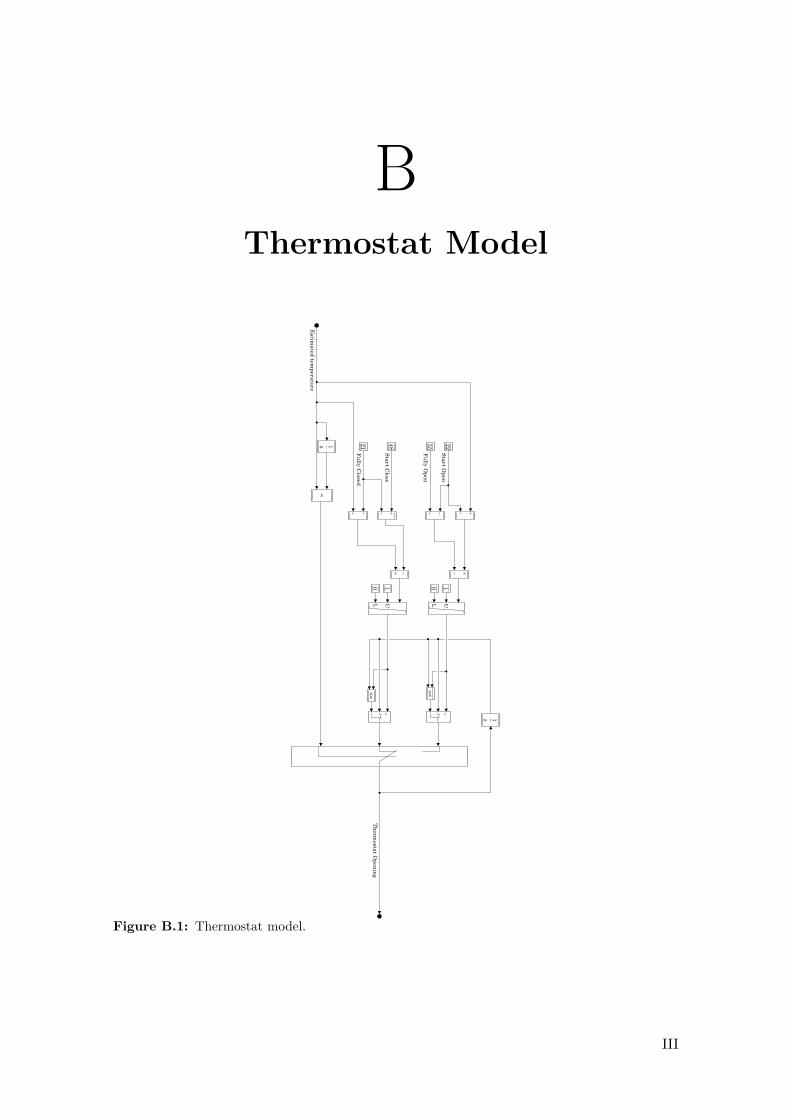
BThermostat Model

1

z 1

z 1

UL UL>=<=

<

21 48 55 22

0 1 0 1

1

Start Open

Fully Open

Start Close

Fully Closed

Thermostat O

pening

Estimated tem

perature

Figure B.1: Thermostat model.

III

Real Time Modeling of Engine Coolant...

Documents

Transcript of Real Time Modeling of Engine Coolant...