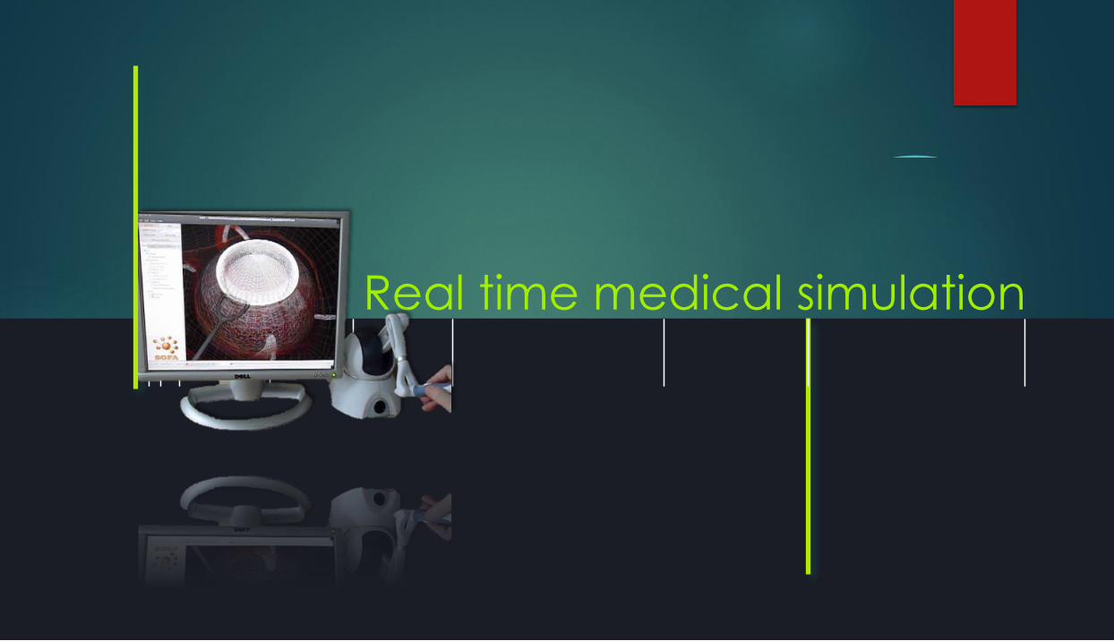
Real time medical simulation
63
Real time medical simulation
Transcript of Real time medical simulation
Real time medical simulation
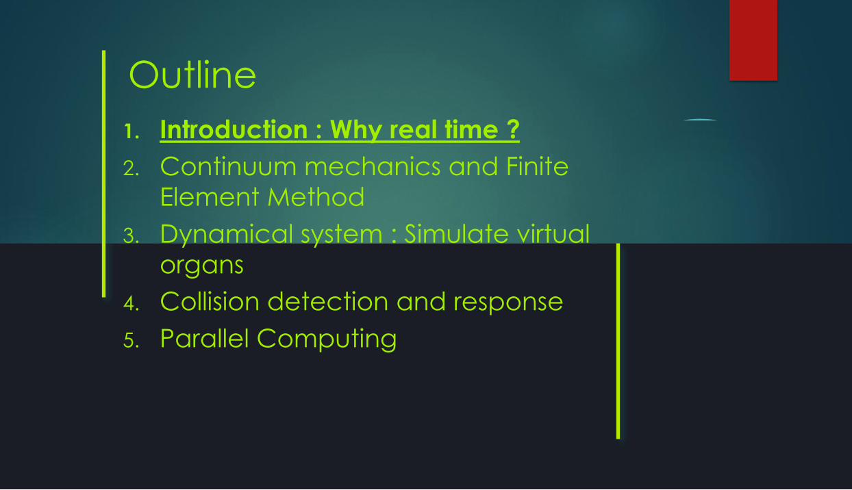
Outline
1. Introduction : Why real time ?
2. Continuum mechanics and Finite
Element Method
3. Dynamical system : Simulate virtual
organs
4. Collision detection and response
5. Parallel Computing
3
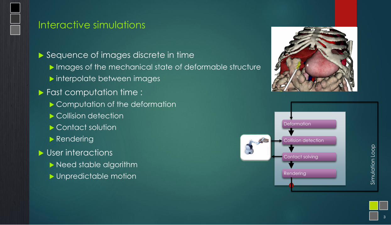
Interactive simulations
Sequence of images discrete in time
Images of the mechanical state of deformable structure
interpolate between images
Fast computation time :
Computation of the deformation
Collision detection
Contact solution
Rendering
User interactions
Need stable algorithm
Unpredictable motion
Deformation
Collision detection
Contact solving
Rendering
Interactions
Sim
ula
tio
n L
oo
p

4
External Forces
Motion
&
Deformation
Physics
computation
___________
Deformable
Rigid
Fluid
No contact
Timet t + dt
Feedback
___________
Visual
Haptic
Tactile
Collision
Detection
___________
Are the objects
in contact?
Conta
ct
Collision
Response
___________
Penalty method
Other Methods
Motion
&
Deformation
Physics
Computation
___________
Reuse the
same physical
modelContact Forces
Contact Forces
Simulation loop

5
Real time : definition
Additional constraints :
A frame rate of at least 60 FPS is necessary to have a visual fluidity
Less than 20 ms to process all the computations (computation of the deformation,
collision detection, contact force response, rendering, …)
Interactive simulation :
A simulation which is not slower than real time but fast enough to allow user interactions
At least 10 FPS
Simulation with haptic feedback
Haptic requires at least 1Khz to simulate a smooth force feedback, ant stiff interactions
Les than 1 ms to update haptic forces
Accuracy ? It’s relatively easy to simulate very fast with very simplified models

6
Strategy for real time
Behavior model
Simple mechanics law (mass spring models, shape matching, linear elasticity, ...)
FEM mesh
Influence directly both : the accuracy and the number of equations solved during a
time step
Temporal integration
Implicit vs. Explicit
Direct/Iterative solvers
Collision detection and contact response
Advanced modulation (friction, unilateral constraints,…)
Code optimizations and parallelism
High parallel architectures (GPU, CPU…)
Find a tradeoff between accuracy and computation time

Outline
1. Introduction : Why real time ?
2. Continuum mechanics and Finite
Element Method
3. Image and meshes : From patient
data to medical simulations
4. Dynamical system : Simulate virtual
organs
5. SOFA : A framework for interactive
medical simualtions

8
Continuum mechanics : basics
Assume a continuity of the matter (true at macroscopic scale, wrong at atomic
scale)
𝛷
Strain tensor
𝝈 Constituve law
휀 = 𝑓(𝜎)
𝜎 = 𝑓−1(휀)
Mechanical model :
• Co-rotational
• Neo Hookean
• MooneyRivlin
• Costa
• ….
No analytical solution for complex structures !
• Strain tensor : measure of the deformation– Cauchy-Green , Green-Lagrange, Euler-Almansi, Biot, Hill
• Stress tensor : measure of the stress
– Cauchy, first Piola Kirchhoff, second Piola Kirchhoff
• Constitutive law : measure of the deformation
– Hooke law, non linear material

9
Equations formulation
Continuum mechanics
Assumption of continuity of matter
Based on physics law
Define a deformation model
Solution based on finite element method
Discretization in small elements
Integrate and solve equations by elements
Approximation which depends on the size of elements
Solution of a dynamic system :
Time evolution of deformable bodies
Involves acceleration, velocity, and position
s Constitutive law
Strain
Str
ess
D
M a = f (p,v)

10
Discretization
Method = receipt how to
discretize the domain and solution
reformulate the differential equations
Digest of current methods
mass-spring damper (MSD)
finite-difference methods (FDM)
boundary element methods (BEM)
finite element method (FEM)
meshless (meshfree) methods

11
Real-time soft tissue deformation :: basic principles
Trade-off between accuracy and computation time
Many possible approaches but often only physically plausible
Physics-based does not mean it is accurate enough for medical training
Most common methods
Mass-spring systems
Finite Element Method
Meshless techniques
Main difference is in the computation of the internal forces
And to some extent the choice of the time integration scheme

12
A simple case: mass-spring models
Example: simulated springs
Particle
mass m, position, velocity
Spring
Rest length l0
Stiffness k
Force f = k(l – l0) with l=(x2 –x1)
Acceleration: a=f/m
Simplest case
One particle, one spring
Theoretical solution
13
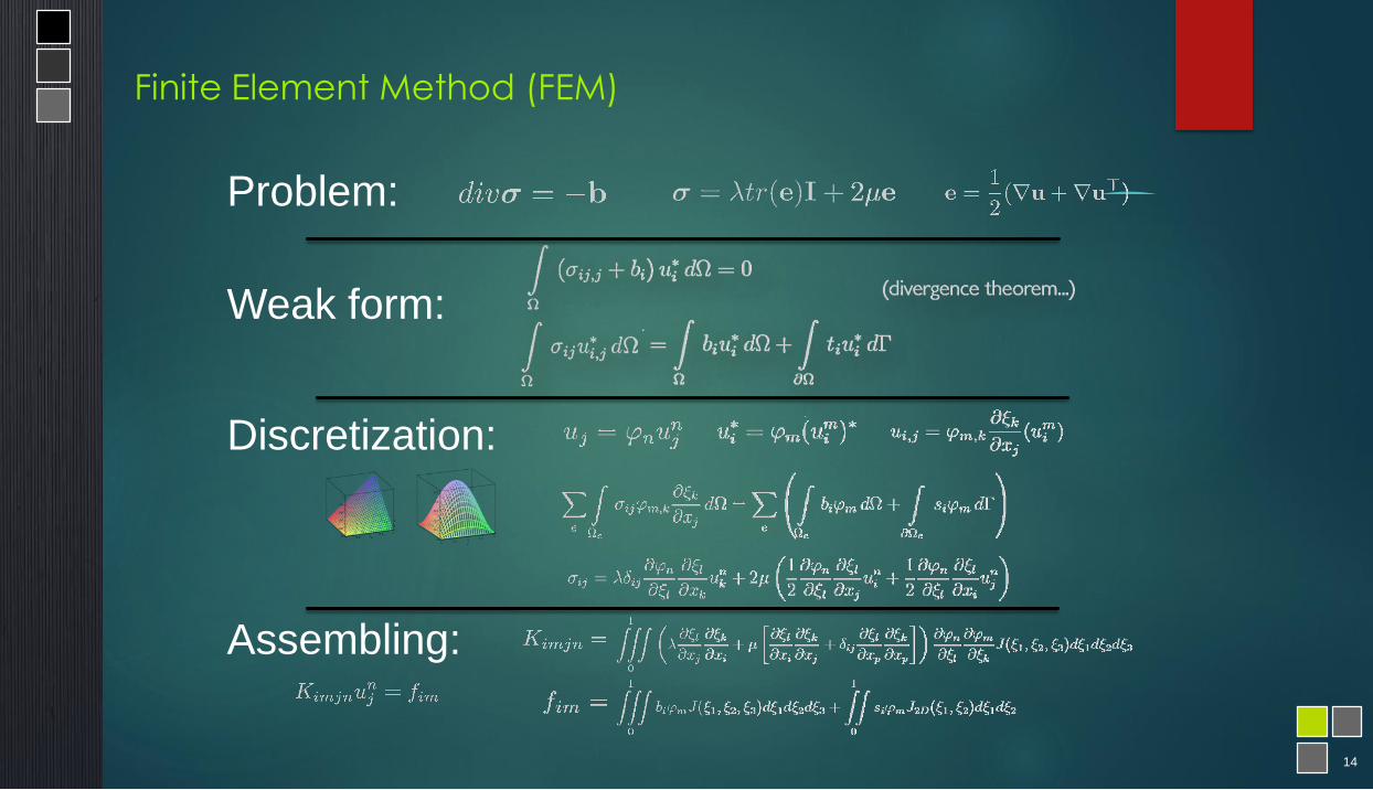
Finite Element Method (FEM)
First appeared in 40s and 50s in civil and aeronautics engineering
Weak formulation of the problem
Multiplication by test function and integration over domain
Discretization of the into elements
Discretization of domain into geometric elements (e.g. simplexes)
Discretization of the equations using shape functions (for the solution and test func.)
Assembly of algebraic system of equations
Results in large sparse matrix
Imposition of the discretized boundary conditions
Several methods (penalty, elimination, Lagrange multipliers)
Numerical solution of the algebraic system
14
Weak form:
Discretization:
Finite Element Method (FEM)
Problem:
Assembling:

15
Discretization methods
Discretization
The first step in creating a physical representation of an object
Choice of discretization method depends on
data dimension (1D, 2D, 3D, 4D...)
input domain geometry (CAD, surface mesh, intensity image)
output type of elements (beams, plates, tetrahedra, hexahedra)
other (available tools/techniques, available hardware, target size/quality/format)

16
Discretization methods
Wide range of algorithms
Tessellations (tiling of a plane)
Delaunay triangulations [DT] (no point of the triangulation lies inside any circumcircle of
any triangle of the triangulation
Voronoi diagrams (dual to DT)
17
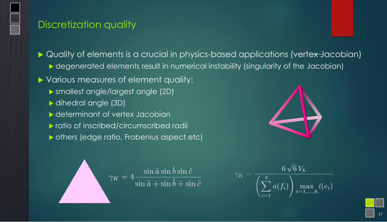
Discretization quality
Quality of elements is a crucial in physics-based applications (vertex Jacobian)
degenerated elements result in numerical instability (singularity of the Jacobian)
Various measures of element quality:
smallest angle/largest angle (2D)
dihedral angle (3D)
determinant of vertex Jacobian
ratio of inscribed/circumscribed radii
others (edge ratio, Frobenius aspect etc)

18
Influence of the mesh
CGAL
Convert a segmented image in a tetrahedral
mesh
Mesh
Discrete representation of the domain
Relation between the degree of freedom
Mesh influence
Computation time (on equation is solved at each
node)
Accuracy (the FEM solution tends toward the
exact solution when the size of elements tends
toward zero).
Fast Accurate
Fast Accurate
Fast Accurate
19
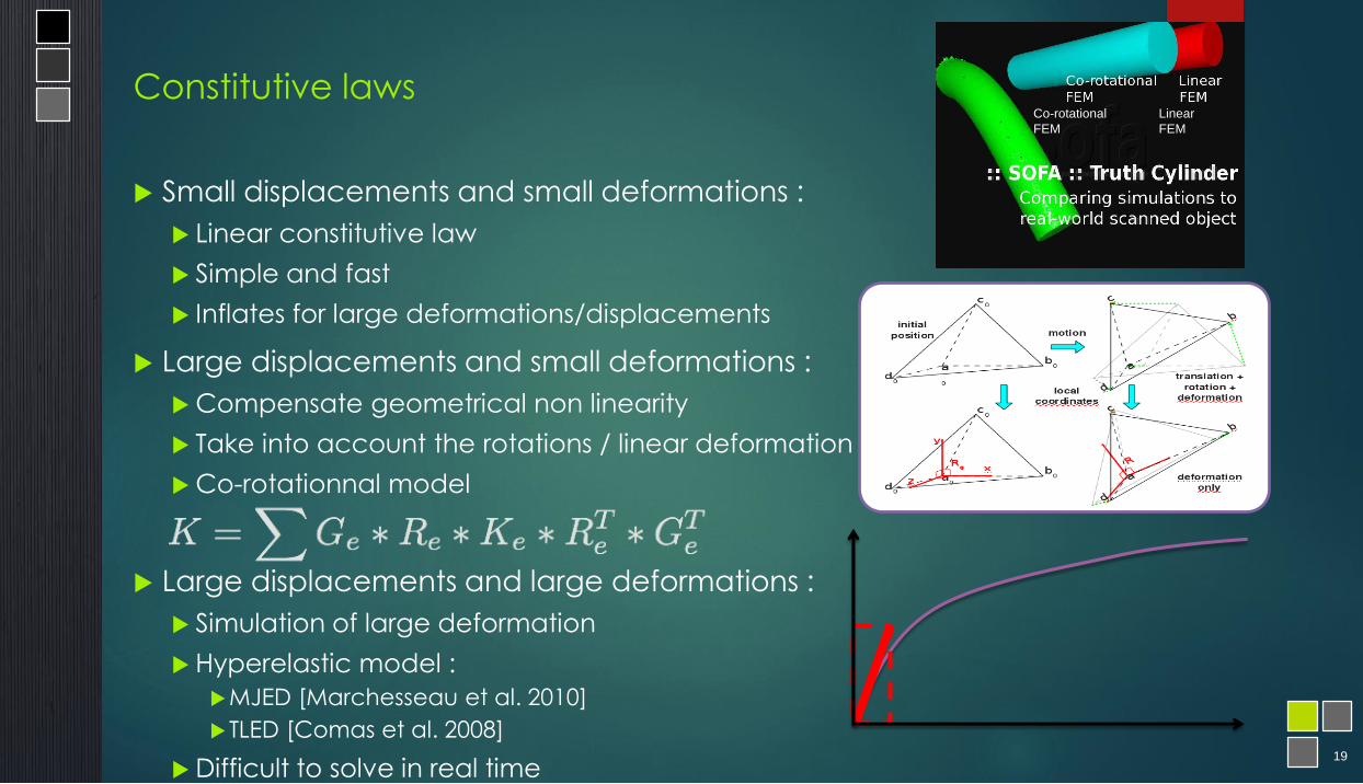
Constitutive laws
Small displacements and small deformations :
Linear constitutive law
Simple and fast
Inflates for large deformations/displacements
Large displacements and small deformations :
Compensate geometrical non linearity
Take into account the rotations / linear deformation
Co-rotationnal model
Large displacements and large deformations :
Simulation of large deformation
Hyperelastic model :
MJED [Marchesseau et al. 2010]
TLED [Comas et al. 2008]
Difficult to solve in real time
Co-rotational
FEM
Linear
FEM

Outline
1. Introduction : Why real time ?
2. Continuum mechanics and Finite
Element Method
3. Dynamical system : Simulate virtual
organs
4. Collision detection and response
5. Parallel Computing
21
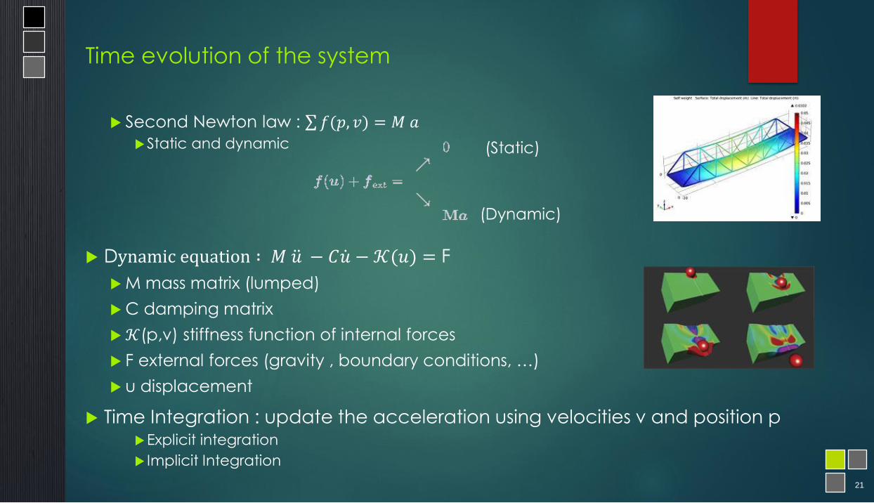
Time evolution of the system
Second Newton law : σ𝑓(𝑝, 𝑣) = 𝑀 𝑎
Static and dynamic
Dynamic equation ∶ 𝑀 ሷ𝑢 − 𝐶 ሶ𝑢 − 𝒦(𝑢) = F
M mass matrix (lumped)
C damping matrix
𝒦(p,v) stiffness function of internal forces
F external forces (gravity , boundary conditions, …)
u displacement
Time Integration : update the acceleration using velocities v and position pExplicit integration
Implicit Integration
(Static)
(Dynamic)

22
Simulation loop
Advancing through time
What appears to be a continuous motion is in fact a sequence of discrete steps
If “dt” is small enough, the motion seems continuous
For smooth visual, dt should be less than 0.04 s (25 FPS)
However, other considerations can have a big impact on the value of “dt”
Time integration
Computing the simulation state at the next time step t+dt given :
State at the current time t: positions xt and velocities vt at each point
Equations and constraints expressing the required mechanics
1. a = a(x,v,t)
2. c(x,v,t) >= 0
How to obtain a fast yet stable simulation?
the choice of the integration scheme is very important
it’s called “integration” as it allows to go from xt to xt or from xt to xt.. . .

23
Explicit integration
Principle : use velocity and acceleration at the beginning of the time-step
Example: forward Euler
at = M-1f
xt+h = xt + hvt with h = dt
vt+h = vt + hat
Main characteristics
Simple
Amplifies motion
Damping is required
Stiff systems require very small time steps

24
Implicit integration
Implicit integration
Principle : use velocity and acceleration at the end of the time-step
Example: backward Euler
Solve
vt+h = vt + hat+h
xt+h = xt + hvt+h
Main characteristics
Complex (requires a solver)
Under-estimates motion
Introduces additional damping
Stable for stiff systems even with large time steps
Well-suited for soft bodies

25
Explicit integration
Principle : compute the acceleration using the position and velocities at the
beginning of the time step
Main properties
Simple (Local solution)
Fast and parallelizable
Amplifies the motion (Need to add damping)
Stability not guarantee (Requires very small time step for stiff objects)
𝒇(𝑝𝑡 , 𝑣𝑡)𝑴𝑎𝑡+ℎ =𝑣𝑡+ℎ = 𝑣𝑡 + ℎ𝑎𝑡+ℎ𝑝𝑡+ℎ = 𝑝𝑡 + ℎ𝑣𝑡+ℎ
Forward Euler :

26
Explicit integration
Critical time step
Conditionally stable = tc exists such that if h < tc then the simulation is stable
For linear behavior models tc = 𝐿
𝑠
L = charasteristic length
s = dilatational wave speed
For tetrahedral elements L = 3𝑉
𝑚𝑎𝑥𝐴with V the volume of the tetrahedra and maxA the largest
area of the 4 triangle of the faces of the tetrahedra
s = 𝐸 ∗1−𝑣
𝑟ℎ𝑜∗ 1 + 𝑣 ∗ (1 − 2𝑣) with rho the mass density, v Poisson coefficient et E le Young
modulus

27
Implicit integration
Principle: Update the acceleration from position and velocity at the end of the
time step
Main properties
Complex (implies to solve a linear system)
Motion is under estimate (Numerical damping)
Stable with large time step and stiff objects (simulation of anatomical structures)
𝒇(𝑝𝑡+ℎ, 𝑣𝑡+ℎ)𝒇(𝑝𝑡 , 𝑣𝑡)
Problem : 𝑝𝑡+ℎand 𝑣𝑡+ℎ are unknown
𝑴𝑎𝑡+ℎ =𝑣𝑡+ℎ = 𝑣𝑡 + ℎ𝑎𝑡+ℎ𝑝𝑡+ℎ = 𝑝𝑡 + ℎ𝑣𝑡+ℎ
Backward Euler

28
Implicit integration
Euler implicit :
𝑢𝑡+ℎ = 𝑢𝑡 + ℎ ሶ𝑢𝑡+ℎ ሶ𝑢𝑡+ℎ = ሶ𝑢𝑡 + ℎ ሷ𝑢𝑡+ℎ
Rearranging gives :
ሶ𝑢𝑡+ℎ =𝑢𝑡+ℎ − 𝑢𝑡
ℎ ሷ𝑢𝑡+ℎ =ሶ𝑢𝑡+ℎ − ሶ𝑢𝑡
ℎ
Dynamic equation :
𝑀 ሷ𝑢𝑡+ℎ − 𝐶 ሶ𝑢𝑡+ℎ −𝒦(𝑢𝑡+ℎ) = 𝑝
𝑀ሶ𝑢𝑡+ℎ − ሶ𝑢𝑡
ℎ− 𝐶
𝑢𝑡+ℎ − 𝑢𝑡ℎ
−𝒦(𝑢𝑡+ℎ) = 𝑝
𝑀𝑢𝑡+ℎℎ2
− 𝐶𝑢𝑡+ℎℎ
−𝒦 𝑢𝑡+ℎ = 𝑝 +𝑀ሶ𝑢𝑡ℎ+𝑀
𝑢𝑡ℎ2
− 𝐶𝑢𝑡ℎ
𝓢 𝑢𝑡+ℎ 𝓕

29
Implicit integration
We want to find 𝑢𝑡+ℎ that equalizes the two members of the equation 𝓢 𝑢𝑡+ℎ = 𝓕
𝓢 𝑢𝑡+ℎ = 𝑀𝑢𝑡+ℎℎ2
− 𝐶𝑢𝑡+ℎℎ
−𝒦 𝑢𝑡+ℎ
𝓕 = 𝑝 +𝑀ሶ𝑢𝑡ℎ+𝑀
𝑢𝑡ℎ2
− 𝐶𝑢𝑡ℎ
For any input parameter 𝑥, we define the residual function
𝑅 𝑥 = 𝓢 𝑥 − 𝓕
The solution is given by 𝑥 such that 𝑅(𝑥) = 0.
𝑅 is still a non linear function.
We use the Newton Raphson algorithm to find the solution
30
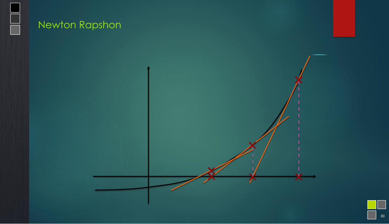
Newton Rapshon

31
Implicit integration
Defining 𝑥(𝑖+1) = 𝑥(𝑖) + 𝛥𝑥(𝑖), 𝑅 𝑥 is linearized as follows :
𝑅𝐿 𝑥(𝑖) + 𝛥𝑥(𝑖) = 𝑅𝐿 𝑥(𝑖) +𝜕𝑅
𝜕𝑥𝑥(𝑖) 𝛥𝑥(𝑖)
Value in 𝑥(𝑖) Tangent in 𝑥(𝑖)
At each iteration we want to find the intersection of the linearized residual function with 0
𝑅𝐿 𝑥(𝑖) +𝜕𝑅𝜕𝑥
𝑥(𝑖) 𝛥𝑥(𝑖) = 0 ⟺ 𝛥𝑥 𝑖 =𝜕𝑅𝜕𝑥
𝑥 𝑖−1
−𝑅𝐿 𝑥 𝑖
Displacement for the next iteration
Replacing in our original problem gives :
𝜕𝓢 𝑥 − 𝓕𝜕𝑥
𝑥 𝑖 𝛥𝑥 𝑖 = 𝓕 − 𝓢 𝑥 𝑖
𝜕𝓕𝜕𝑥
𝑥 𝑖 = 0with
⟺𝜕𝓢 𝑥𝜕𝑥
𝑥 𝑖 𝛥𝑥 𝑖 = 𝓕 − 𝓢 𝑥 𝑖

32
Implicit integration
𝜕𝓢 𝑥𝜕𝑥
𝑥 𝑖 𝛥𝑥 𝑖 = 𝓕 − 𝓢 𝑥 𝑖
𝓢 𝑥 = 𝑀𝑥
ℎ2− 𝐶
𝑥
ℎ−𝒦 𝑥
𝓕 = 𝑝 +𝑀ሶ𝑢𝑡ℎ+𝑀
𝑢𝑡ℎ2
− 𝐶𝑢𝑡ℎ
Mechanical equation
Linearized problem
Combining equations gives :
𝑀
ℎ2−𝐶
ℎ−
𝜕𝒦 𝑥𝜕𝑥
𝑥 𝑖 𝑥(𝑖+1) − 𝑥(𝑖) = 𝓕 −𝑀
ℎ2−𝐶
ℎ𝑥 𝑖 +𝒦 𝑥 𝑖
𝛥𝑥(𝑖) = 𝑥(𝑖+1) − 𝑥(𝑖)Newton increment
𝑀
ℎ2−𝐶
ℎ−
𝜕𝒦 𝑥𝜕𝑥
𝑥 𝑖 𝑥(𝑖+1) = 𝓕 −𝑀
ℎ2−𝐶
ℎ𝑥 𝑖 +𝒦 𝑥 𝑖 +
𝑀
ℎ2−𝐶
ℎ−
𝜕𝒦 𝑥𝜕𝑥
𝑥 𝑖 𝑥(𝑖)
33
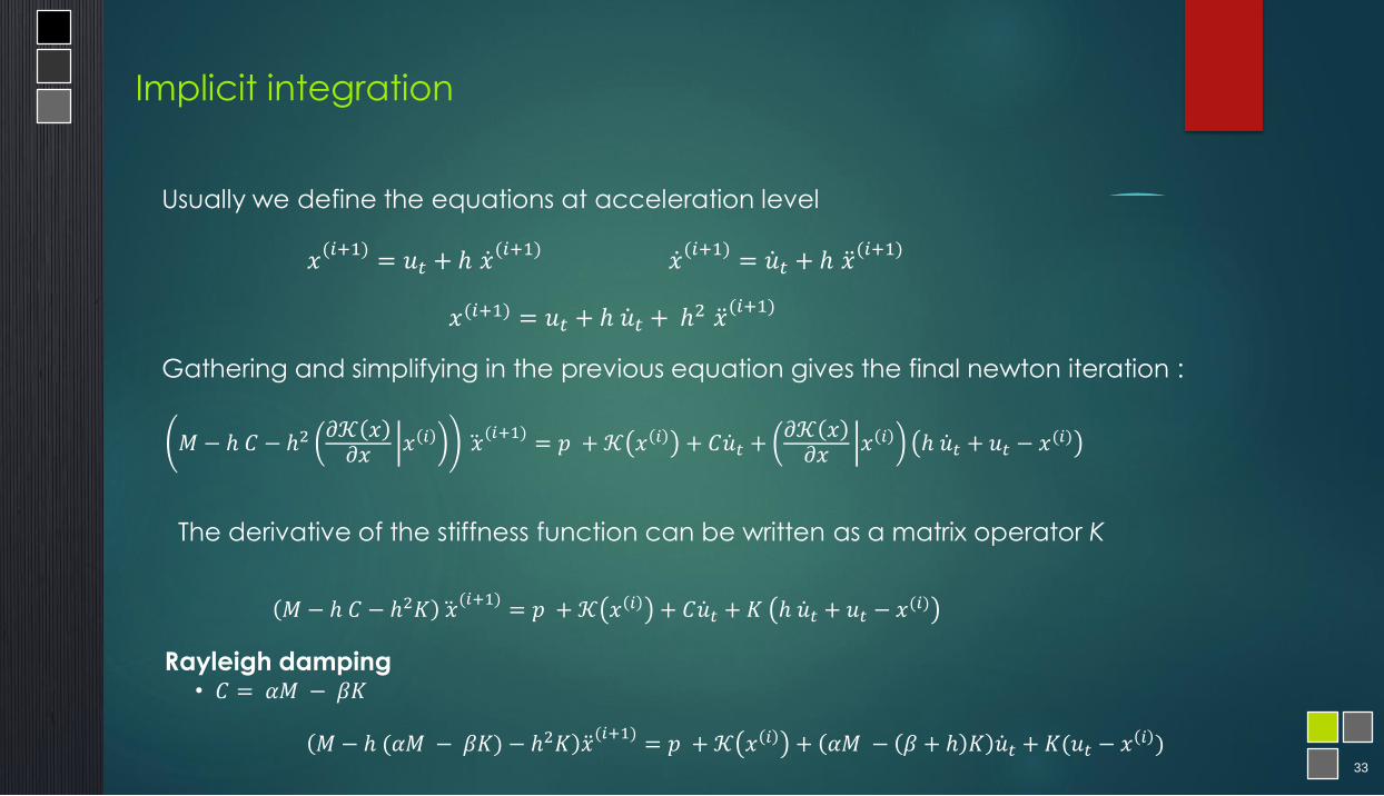
Implicit integration
Usually we define the equations at acceleration level
𝑥(𝑖+1) = 𝑢𝑡 + ℎ ሶ𝑢𝑡 + ℎ2 ሷ𝑥(𝑖+1)
𝑥(𝑖+1)
= 𝑢𝑡 + ℎ ሶ𝑥(𝑖+1)
ሶ𝑥(𝑖+1)
= ሶ𝑢𝑡 + ℎ ሷ𝑥(𝑖+1)
Gathering and simplifying in the previous equation gives the final newton iteration :
𝑀 − ℎ 𝐶 − ℎ2𝜕𝒦 𝑥𝜕𝑥
𝑥 𝑖 ሷ𝑥(𝑖+1)
= 𝑝 +𝒦 𝑥 𝑖 + 𝐶 ሶ𝑢𝑡 +𝜕𝒦 𝑥𝜕𝑥
𝑥 𝑖 ℎ ሶ𝑢𝑡 + 𝑢𝑡 − 𝑥(𝑖)
The derivative of the stiffness function can be written as a matrix operator K
𝑀 − ℎ 𝐶 − ℎ2𝐾 ሷ𝑥(𝑖+1)
= 𝑝 +𝒦 𝑥 𝑖 + 𝐶 ሶ𝑢𝑡 + 𝐾 ℎ ሶ𝑢𝑡 + 𝑢𝑡 − 𝑥(𝑖)
Rayleigh damping• 𝐶 = 𝛼𝑀 − 𝛽𝐾
𝑀 − ℎ (𝛼𝑀 − 𝛽𝐾) − ℎ2𝐾 ሷ𝑥(𝑖+1)
= 𝑝 +𝒦 𝑥 𝑖 + 𝛼𝑀 − 𝛽 + ℎ 𝐾 ሶ𝑢𝑡 + 𝐾(𝑢𝑡 − 𝑥 𝑖 )
34
ሼ
𝑨 𝒙 = 𝒃
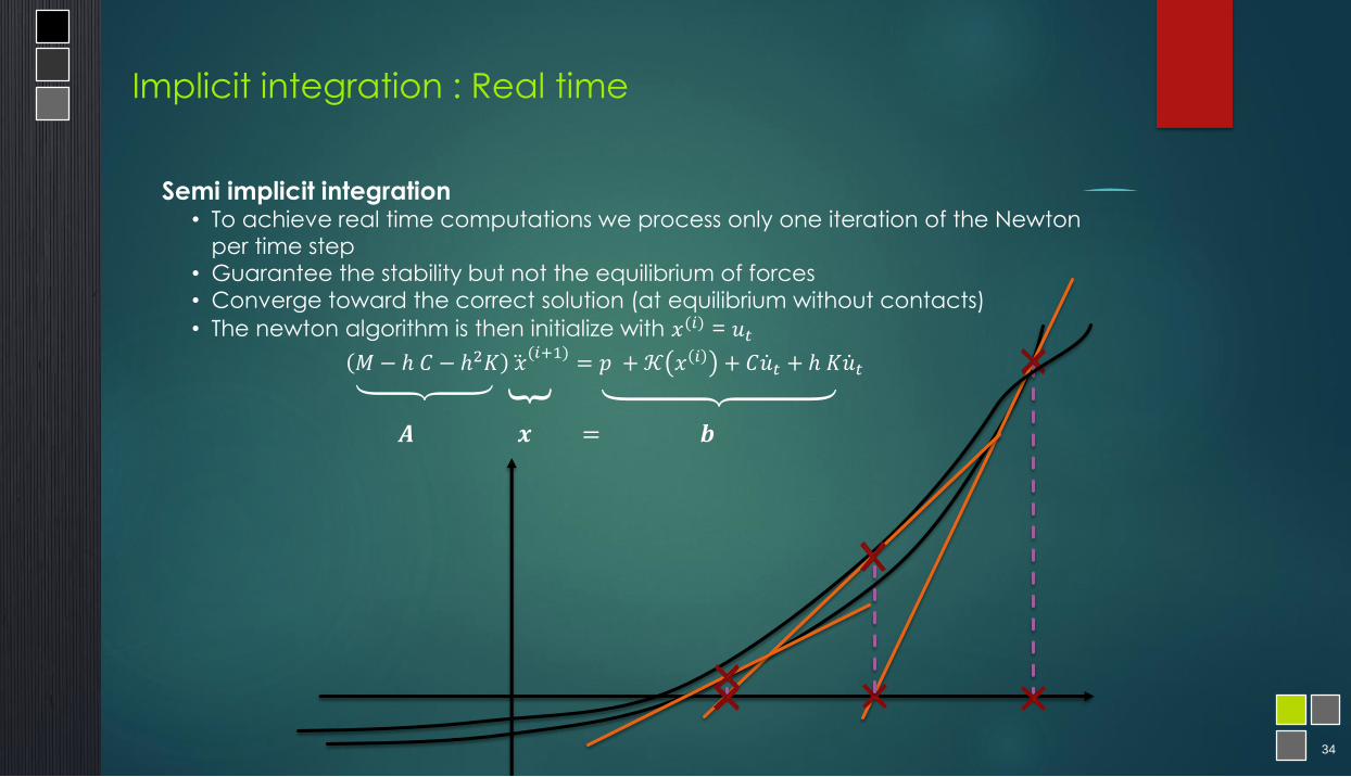
Semi implicit integration • To achieve real time computations we process only one iteration of the Newton
per time step
• Guarantee the stability but not the equilibrium of forces
• Converge toward the correct solution (at equilibrium without contacts)
• The newton algorithm is then initialize with 𝑥(𝑖) = 𝑢𝑡
𝑀 − ℎ 𝐶 − ℎ2𝐾 ሷ𝑥(𝑖+1)
= 𝑝 +𝒦 𝑥 𝑖 + 𝐶 ሶ𝑢𝑡 + ℎ 𝐾 ሶ𝑢𝑡
Implicit integration : Real time

35
1
4567
0 1 2 3 4 5 6 7
123
0 b c db e fc g h i jd f h k l m
i n o
a
j l o p q rm q s t
r t u
01
2 3
4
5
6
7
A is :• Directly obtained from the mesh structure• Sparse• Symmetric
• Positive definite
Direct solvers : • Direct inverse (dense)
• Factorization :
• A = LU • A = 𝐿𝐿𝑡 (cholesky)
• A = 𝐿𝐷𝐿𝑡Gauss elimination
Iterative solvers : • Refine a solution. Converge toward the correct
solution
• Gauss-Seidel• Jacobi
• Conjugate Gradient
Accurate / slow, expensive in memory
Approximation/ fast
Implicit integration : Real time

36
1
4567
0 1 2 3 4 5 6 7
123
0 b c db e fc g h i jd f h k l m
i n o
a
j l o p q rm q s t
r t u
01
2 3
4
5
6
7
0 1 2 3 0 1 3 0 2 3 4 5 0 1 2 3 5 6 2 4 5 2 3 4 5 6 7 3 5 6 7 5 6 7
0 4 7 12 18 21 27 31 34
a b c d b e f c g h i j d f h k l m i n o j l o p q r m q s t r t u
Row Pointer
Column Pointer
Values
Compressed Row Sparse format

37
Suppose we want to solve the following system of linear equations
Ax = b
for the vector x where the known n-by-n matrix A is symmetric (i.e. AT = A), positive
definite (i.e. xTAx > 0 for all non-zero vectors x in Rn), and real, and b is known as
well.
We say that two non-zero vectors u and v are conjugate (with respect to A) if
Since A is symmetric and positive definite, the left-hand side defines an inner
product
Two vectors are conjugate if they are orthogonal with respect to this inner
product. Being conjugate is a symmetric relation: if u is conjugate to v, then v is
conjugate to u.
Implicit integration : Conjugate Gradient

38
Suppose that is a set of n mutually conjugate
directions. Then is a basis of , so within we can expand the solution of
and we see that
For any
(because are mutually conjugate)
Find a sequence of n conjugate directions, and then compute the coefficients .
Implicit integration : Conjugate Gradient

39
Let rk be the residual at the kth step:
The CG algorithm relies on a Gram-Schmidt orthonormalization. This gives the following expression:
Following this direction, the next optimal
location is given by
The is chosen such that is
conjugated to . Initially, is
Implicit integration : Conjugate Gradient

40
ODE Solver
Non linear Solver
linear Solver
Euler implicitEuler explicitRunge Kutta
Verlet
Newton-Raphson
Conjugate GradientCholesky SolverDirecte inverse
Implicit integration : Solverse

41
Summary on time integration schemes
Two main types
Explicit and implicit
Many methods (Euler, Runge Kutta, Leap Frog, Verlet, ...)
All have benefits and drawbacks
The choice depends on the application
Mainly
explicit methods: conditionally stable, i.e. depends on time step dt
implicit methods: unconditionally stable, i.e. do not (entirely) depend on time step dt
Other considerations include energy loss or gain

42
Real time : definition
A simulation is real-time if all the computations done in 1 time step are done in a
time equal to the time step.
The number of Frame Per Second (FPS) times dt must be equal to 1 second.
dt
t t+dt
Simulation
time
t+1sec
User time
(real)
t+1sect

43
Real time : definition
Simulation too fast:
Slow down the simulation with a waiting loop
dt
t t+dt t+1sec
t+1sect
t+1sec
Simulation
time
User time
(real)

44
Real time : definition
Simulation too slow :
Record the images of the simulation, and play them faster to reach real time.
Impossible when the user interact with the simulation !
dt
t t+dt t+1sec
t+1sect
Simulation
time
User time
(real)

45
Real time : definition
Synchronize the simulated instruments with the simulated bodies
Slow down the motion of the instruments in the simulation
Difficult (impossible) to use for a surgeon
Delay when applying haptic forces
Real motion Simulation
Deformabl
eStructure
(slow)

46
Real time : definition
Synchronize the simulated instruments with the user motion
The velocity of the instruments is faster than other deformable structures
Important error introduced during the interaction
Real motion Simulation
Structure
déformable
Deformabl
eStructure
(slow)

47
Real time : definition
Crash test example :
The velocity has a huge impact on the resulting deformation
Delay in the simulation introduce important errors !
Outline
1. Introduction : Why real time ?
2. Continuum mechanics and Finite
Element Method
3. Dynamical system : Simulate virtual
organs
4. Collision detection and response
5. Parallel Computing

49
Collision Detection
Stable modeling of interactions between objects in real-time simulation
Determination of collision area
Computation of collision volume
Needs to be :
Fast for real-time simulation
Accurate for computation of contact forces
49
Collision volume

50
Collision Detection
Deciding what to test hat to test
Applying tests Applying tests
Determining whether a collision occurred
Determining when a collision occurred
Determining where a collision occurred
Broad-phase: select pairs for comparison
Goals:
Make selections quickly
Avoid selecting objects that can’t collide
Narrow-phase: compare individual pairs
Goals:
Accurate comparisons
Efficient comparisons

51
Collision Detection
Convex Polygon Test
Test point has to be on same side of all edge
Point/Sphere
Simplest 3D Bounding Volume
Center point and radius
Point in/out test: Calculate distance between test point and center point
If distance <= radius, point is inside
Axis-Aligned Bounding Boxes (AABB)
51

52
Mapping
Collision detection must be accurate
One sphere is not enough
Collision test are expensive
Use simplified mesh
Mapping:
Link between mechanical and collision mesh (both side)
Linear (or not) relation
Use barycentric coordinates
Area of a tetrahedron:
f the origin of the coordinate system is chosen to coincide with vertex d, then d = 0, so

53
Constraints
Penalty-based methods
Add springs between objects
Fast/simple
Object are coupled (slow)
Stiff contact are unstable (interpenetrations)
Augmented lagragian approach
Add new equations
Enforce non interpenetrations
Direct solver :
Coupled system (large)
Ill conditioned (lagrangian multipliers are not mechanical dofs)
53
B
A
A
B
J1
J1T
X1 B1
X2 B2
𝜆 𝛿
J2
J2T
𝐴 0 𝐽10 𝐵 𝐽2𝐽1𝑇 𝐽2
𝑇 0
𝑥1𝑥2𝜆
=𝑏1𝑏2𝛿

54
Validation of the method
Compare the positions with different approximations of the Compliance
The green shape represent the exact solution
The object is non homogeneous : Red tetrahedra are stiffer than blue ones
With Asynchronous update of the preconditioner, we get almost the correct
solution
The green part and the blue part overlap perfectly
54
dt=0,01
Update every 3 time steps on
average
dt=0,01
Complia
nce
Warping
dt=0,01
Update
every 50
time steps
dt=0,01
Update
every 20
time steps
55
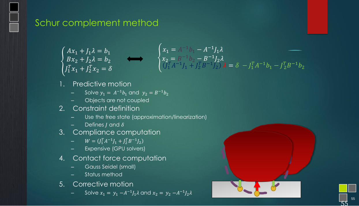
Schur complement method
55
൞
𝐴𝑥1 + 𝐽1𝜆 = 𝑏1𝐵𝑥2 + 𝐽2𝜆 = 𝑏2𝐽1𝑇𝑥1 + 𝐽2
𝑇𝑥2 = 𝛿
൞𝑥1 = 𝐴−1𝑏1 − 𝐴−1𝐽1𝜆
𝑥2 = 𝐵−1𝑏2 − 𝐵−1𝐽2𝜆
1. Predictive motion– Solve 𝑦1 = 𝐴−1𝑏1 and 𝑦2 = 𝐵−1𝑏2– Objects are not coupled
𝐽1𝑇𝐴−1𝐽1 + 𝐽2
𝑇𝐵−1𝐽2 𝜆 = 𝛿 − 𝐽1𝑇𝐴−1𝑏1 − 𝐽2
𝑇𝐵−1𝑏2
2. Constraint definition– Use the free state (approximation/linearization)
– Defines 𝐽 and 𝛿
3. Compliance computation– 𝑊 = 𝐽1
𝑇𝐴−1𝐽1 + 𝐽2𝑇𝐵−1𝐽2
– Expensive (GPU solvers)
4. Contact force computation– Gauss Seidel (small)
– Status method
5. Corrective motion– Solve 𝑥1 = 𝑦1 −𝐴
−1𝐽1𝜆 and 𝑥2 = 𝑦2 −𝐴−1𝐽2𝜆

56
Haptic with hyperelastic models (Iros 2015)
56
• Asynchronous computation:1. Sparse factorization of the system is updated at low rate (10 – 20 Hz)
2. Haptic loop update the contact problem at high rate (1 Khz)
Simulation
Loop
(30-100 Hz)
Compliance
Loop
(1-10 Hz)
A
L,D
Haptic Loop
(500-1000 Hz)δW, H

Outline
1. Introduction : Why real time ?
2. Continuum mechanics and Finite
Element Method
3. Dynamical system : Simulate virtual
organs
4. Collision detection and response
5. Parallel Computing

58
New parallel architectures
Difficult to increase the frequency of processors
Heat dissipation
Electric consumption
Parallelization of algorithms
Parallelization of a simulation is not a new idea :
Parallel processors, distributed processors, …
Real time simulation constraints :
A lot of very fast computations
Use GPU to achieve computations (GPGPU).
GPU is very different than CPU parallelization.
Run thousand of threads to exploit efficiently the GPU
GPU is seen as a specialized co-processeur :
Achieve high parallel tasks
58

59
Multi-CPU using KAAPI
How to optimize the use of current hardware architectures (multi-core)
Change the control of
execution in the SOFA core
transparent to components
transparent to (most) solver
Main research contribution:
iterative extensions to task
graphs
A supported feature in
the next public release
5
9

60
GPU architecture
GPU is seen as a specialized co-processeur :
Achieve high parallel tasks
Two level of parallelism :
A Grid contains several blocs
A Block contains several threads
GPU programing :
Local synchronisations very fast
Global synchronisations very slow
(Synchronisation with the CPU)
Run thousand of threads of threads to exploit
efficiently the GPU !60
CPU
Kernel 1
GPU
Grille 1
Block
(0,0)
Block
(1,0)
Blobk
(2,0)
Block
(0,1)
Block
(1,1)
Block
(1,2)
Grille 2Kernel 2
Block (1,1)
Thread
(0,0)Thread
(1,0)Thread
(2,0)Thread
(3,0)Thread
(4,0)
Thread
(0,1)
Thread
(1,1)
Thread
(2,1)
Thread
(3,1)
Thread
(4,1)
Thread
(0,2)
Thread
(1,2)
Thread
(2,2)
Thread
(3,2)
Thread
(4,3)

61
Performances evaluation
Speedup between 5 to 25
Simulate 300 000 elements in real time (CG limited to 25 iterations)
Nombre
Number of elements
Speedup

62
Parallel Computing for Interactive Applications
Main challenges
Leverage new multi-core architectures (CPUs and GPUs)
Large potential but difficult to exploit
New parallel architectures
Programming is still complex (no unique language, no standard, ...)
Simplify the development process (transparency)
Adaptive and multilevel computations
Develop dedicated algorithms (from serial to parallel)
Different levels of parallelization (simulation level, object level)
6
2
62
63
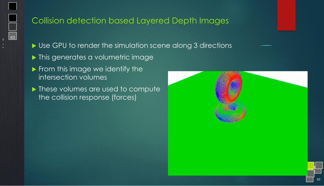
Collision detection based Layered Depth Images
Use GPU to render the simulation scene along 3 directions
This generates a volumetric image
From this image we identify the intersection volumes
These volumes are used to compute
the collision response (forces)
6
3
63