Real-time anomaly detection in logs using rule mining and ...

Real-time anomaly detection in logs usingrule mining and complex event processing

at scale

DELFT UNIVERSITY OF TECHNOLOGY

MASTERS THESIS


at scale

Author:Alexandros STAVROULAKIS

Supervisor:Asterios KATSIFODIMOS

A thesis submitted in fulfillment of the requirementsfor the degree of Master of Science

in the

Web Information Systems GroupSoftware Technology

August 11, 2019

http://www.tudelft.nl

http://www.wis.ewi.tudelft.nl/

https://www.tudelft.nl/en/eemcs/the-faculty/departments/software-technology/

iii

Declaration of AuthorshipI, Alexandros STAVROULAKIS, declare that this thesis titled, “Real-time anomaly de-tection in logs using rule mining and complex event processing at scale” and thework presented in it are my own. I confirm that:

• This work was done wholly or mainly while in candidature for a research de-gree at this University.

• Where any part of this thesis has previously been submitted for a degree orany other qualification at this University or any other institution, this has beenclearly stated.

• Where I have consulted the published work of others, this is always clearlyattributed.

• Where I have quoted from the work of others, the source is always given. Withthe exception of such quotations, this thesis is entirely my own work.

• I have acknowledged all main sources of help.

• Where the thesis is based on work done by myself jointly with others, I havemade clear exactly what was done by others and what I have contributed my-self.

Signed:

Date:

An electronic version of this thesis is available athttp://repository.tudelft.nl/.

http://repository.tudelft.nl/

Alexandros Stavroulakis

12/08/2019

v


at scale

Abstract

Author: Alexandros StavroulakisStudent ID: 4747933Email: [email protected]

Log data, produced from every computer system and program, are widely usedas source of valuable information to monitor and understand their behavior andtheir health. However, as large-scale systems generate a massive amount of log dataevery minute, it is impossible to detect the cause of system failure by examiningmanually this huge size of data. Thus, there is a need for an automated tool forfinding system’s failure with little or none human effort.

Nowadays lots of methods exist that try to detect anomalies on system’s logs byanalyzing and applying various algorithms such as machine learning algorithms.However, experts argue that a system error can not be found by looking into a singleevent, but in multiple log event data are necessary to understand the root cause of aproblem.

In this thesis work, we aim to detect patterns in sequential distributed system’slogs that can capture effectively the abnormal behavior. Specifically as a first step,we will apply rule mining techniques to extract rules that represent an anomalousbehavior, which potentially in the future may lead to a failure of a system. Exceptfor that step, we implemented a real-time anomaly detection framework to detectproblems before they actually occur.

Processing log data as streams is the only way to achieve a real-time detectionconcept. In that direction we will process streaming log data using a complex eventprocessing technique. Specifically, we would like to combine rule mining algorithmswith complex event processing engine to raise alerts on abnormal log data basedon automatically generated patterns. The evaluation of the work is conducted onHadoop’s logs, a widely used system in the industry. The outcome of this thesisproject gives really promising results, reaching a Recall of 98% in detecting anoma-lies. Finally, a scalable anomaly detection framework was build by integrating dif-ferent systems into the cloud. The motivation behind this is the direct application ofour framework to a real-life use case.

Thesis Committee:

Chair: Prof. Dr. ir. Alessandro Bozzon, Faculty EEMCS, TU DelftUniversity Supervisor: Dr. Asterios Katsifodimos, Faculty EEMCS, TU DelftCompany Supervisor: Mr. Riccardo Vincelli, KPMGCommittee Member: Dr. Mauricio Aniche, Faculty EEMCS, TU Delft

vii

AcknowledgementsWith the submission of this thesis I not only finishing my Master studies in Com-

puter Science at Delft University of Technology, but I also conclude my student life.During this time I have been improved both as a scientist and as a person, by over-coming the challenges that I was facing. However the completion of this work wouldnot have been possible without the help of many people that I want to thank.

First of all I want to thank my supervisor, Asterios Katsifodimos, for his endlesshelp. His door was always open for me to listen to my problems and my crazysolutions. From the early stages of finding the thesis topic till the end of the work,his guidance was more than helpful and his expertise was crucial on lots of aspects.

Since this thesis was carried out as an internship in KPMG, I was really happythat I had a second supervisor from the company’s side. Riccardo Vincelli thankyou very much for your continuous support and guidance throughout the past ninemonths. With your experience and your enthusiasm we managed to overcome to-gether lots of difficulties that I faced during this work. Thank you for spendingmuch of your time with me, to listen to my issues and proposing interesting andhelpful solutions.

I want to thank all my colleagues at KPMG for their help. Everyone helped a lotby listening and answering random questions that I had since they had experiencein both engineering and research fields. Also I want to thank you all for welcomingme as a member of your team and making my time there very enjoyable.

Finally, I want to thank all my friends and my family for their unconditional sup-port, not only during the past months, but during my whole student life. Withoutthem it would be impossible to succeed.

ix

Contents

Declaration of Authorship iii

Abstract v

Acknowledgements vii

1 Introduction 11.1 Motivation . . . . . . . . . . . . . . . . . . . . . . . . . . . . . . . . . . . 11.2 Research Questions . . . . . . . . . . . . . . . . . . . . . . . . . . . . . . 21.3 Dataset . . . . . . . . . . . . . . . . . . . . . . . . . . . . . . . . . . . . . 21.4 Outline . . . . . . . . . . . . . . . . . . . . . . . . . . . . . . . . . . . . . 3

2 Literature Review 52.1 Background . . . . . . . . . . . . . . . . . . . . . . . . . . . . . . . . . . 5

2.1.1 Log Analysis . . . . . . . . . . . . . . . . . . . . . . . . . . . . . 52.1.2 Complex Event Processing . . . . . . . . . . . . . . . . . . . . . 52.1.3 Rule Mining . . . . . . . . . . . . . . . . . . . . . . . . . . . . . . 6

Definition . . . . . . . . . . . . . . . . . . . . . . . . . . . . . . . 62.2 Related Work . . . . . . . . . . . . . . . . . . . . . . . . . . . . . . . . . 7

2.2.1 Real-time log analysis . . . . . . . . . . . . . . . . . . . . . . . . 7Log analysis at scale . . . . . . . . . . . . . . . . . . . . . . . . . 8

2.2.2 Anomaly detection in logs . . . . . . . . . . . . . . . . . . . . . . 92.2.3 Pattern mining in logs . . . . . . . . . . . . . . . . . . . . . . . . 92.2.4 Complex Event Processing in Logs . . . . . . . . . . . . . . . . . 102.2.5 Automated Complex Event Processing . . . . . . . . . . . . . . 11

3 Case study: Anomaly detection on distributed file-system logs 153.1 General pipeline . . . . . . . . . . . . . . . . . . . . . . . . . . . . . . . . 153.2 Data pre-processing . . . . . . . . . . . . . . . . . . . . . . . . . . . . . . 163.3 Datasets generation . . . . . . . . . . . . . . . . . . . . . . . . . . . . . . 183.4 Metrics definition . . . . . . . . . . . . . . . . . . . . . . . . . . . . . . . 19

4 Anomaly detection on patterns using rule mining techniques 214.1 Dataset . . . . . . . . . . . . . . . . . . . . . . . . . . . . . . . . . . . . . 224.2 Method 1: Association rule mining . . . . . . . . . . . . . . . . . . . . . 224.3 Method 2: Sequential rule mining . . . . . . . . . . . . . . . . . . . . . . 254.4 Method 3: Sliding window and Sequential rule mining . . . . . . . . . 26

5 Rule transformation to complex event processing 315.1 Rules generator . . . . . . . . . . . . . . . . . . . . . . . . . . . . . . . . 315.2 Automate complex event processing engine . . . . . . . . . . . . . . . . 315.3 Flink job configuration . . . . . . . . . . . . . . . . . . . . . . . . . . . . 33

x

6 Experiments and Results 376.1 Baseline Experiment . . . . . . . . . . . . . . . . . . . . . . . . . . . . . 376.2 Effect of number of messages per block . . . . . . . . . . . . . . . . . . 386.3 Necessary number of abnormal data . . . . . . . . . . . . . . . . . . . . 396.4 Experiment to improve Precision . . . . . . . . . . . . . . . . . . . . . . 406.5 Algorithm computational complexity analysis . . . . . . . . . . . . . . 416.6 Comparison with similar works . . . . . . . . . . . . . . . . . . . . . . . 42

7 Scaling out anomaly detection in the cloud 437.1 Pipeline . . . . . . . . . . . . . . . . . . . . . . . . . . . . . . . . . . . . . 43

7.1.1 Data flow . . . . . . . . . . . . . . . . . . . . . . . . . . . . . . . 437.2 Large scale configuration . . . . . . . . . . . . . . . . . . . . . . . . . . . 44

7.2.1 Scaling system . . . . . . . . . . . . . . . . . . . . . . . . . . . . 447.2.2 Containers . . . . . . . . . . . . . . . . . . . . . . . . . . . . . . . 457.2.3 Log collector . . . . . . . . . . . . . . . . . . . . . . . . . . . . . . 467.2.4 Message sink . . . . . . . . . . . . . . . . . . . . . . . . . . . . . 477.2.5 Streaming processing . . . . . . . . . . . . . . . . . . . . . . . . . 497.2.6 Rule generator and log publisher . . . . . . . . . . . . . . . . . . 50

8 Discussion and Conclusion 538.1 Discussion . . . . . . . . . . . . . . . . . . . . . . . . . . . . . . . . . . . 538.2 Limitations . . . . . . . . . . . . . . . . . . . . . . . . . . . . . . . . . . . 548.3 Conclusion and further improvements . . . . . . . . . . . . . . . . . . . 55

Bibliography 57

xi

List of Figures

1.1 Raw HDFS data . . . . . . . . . . . . . . . . . . . . . . . . . . . . . . . . 3

3.1 General Pipeline . . . . . . . . . . . . . . . . . . . . . . . . . . . . . . . 163.2 Raw log message . . . . . . . . . . . . . . . . . . . . . . . . . . . . . . . 163.3 Data pre-processing pipeline . . . . . . . . . . . . . . . . . . . . . . . . 183.4 Grouped dataset . . . . . . . . . . . . . . . . . . . . . . . . . . . . . . . . 18

4.1 Classification of frequent itemsets Pipeline . . . . . . . . . . . . . . . . 214.2 Messsages per bins of 30 seconds . . . . . . . . . . . . . . . . . . . . . . 264.3 Bayesian optimization for sliding window size and support factor . . . 284.4 Minimum number of message in normal and abnormal blocks . . . . . 29

5.1 Rules generator Pipeline . . . . . . . . . . . . . . . . . . . . . . . . . . . 325.2 Flink job execution graph . . . . . . . . . . . . . . . . . . . . . . . . . . 335.3 Input log data . . . . . . . . . . . . . . . . . . . . . . . . . . . . . . . . . 345.4 Final alerts of Flink CEP job . . . . . . . . . . . . . . . . . . . . . . . . . 345.5 Different notions of time in Flink streaming processing . . . . . . . . . 35

6.1 Experiments with different size of abnormal dataset in training phase 396.2 Runtime experiments . . . . . . . . . . . . . . . . . . . . . . . . . . . . 41

7.1 Framework Structure . . . . . . . . . . . . . . . . . . . . . . . . . . . . . 447.2 Kubernetes . . . . . . . . . . . . . . . . . . . . . . . . . . . . . . . . . . . 457.3 Docker . . . . . . . . . . . . . . . . . . . . . . . . . . . . . . . . . . . . . 467.4 FluentD . . . . . . . . . . . . . . . . . . . . . . . . . . . . . . . . . . . . . 477.5 Apache Kafka . . . . . . . . . . . . . . . . . . . . . . . . . . . . . . . . . 487.6 Zookeeper . . . . . . . . . . . . . . . . . . . . . . . . . . . . . . . . . . . 497.7 Flink . . . . . . . . . . . . . . . . . . . . . . . . . . . . . . . . . . . . . . 50

xiii

List of Tables

1.1 Hadoop File System Data . . . . . . . . . . . . . . . . . . . . . . . . . . 2

2.1 Rule mining example . . . . . . . . . . . . . . . . . . . . . . . . . . . . . 6

3.1 Message representation to numbers . . . . . . . . . . . . . . . . . . . . 17

4.1 ARM results, without itemset comparison . . . . . . . . . . . . . . . . . 234.2 ARM results, with itemset comparison . . . . . . . . . . . . . . . . . . . 244.3 Association rule frequent itemsets . . . . . . . . . . . . . . . . . . . . . 244.4 SRM results, without itemset comparison . . . . . . . . . . . . . . . . . 254.5 SRM results, with itemset comparison . . . . . . . . . . . . . . . . . . . 264.6 Sliding Window data . . . . . . . . . . . . . . . . . . . . . . . . . . . . . 284.7 SRM results, with sliding window . . . . . . . . . . . . . . . . . . . . . 29

6.1 Results from Baseline experiment . . . . . . . . . . . . . . . . . . . . . . 376.2 Metrics of Baseline experiment . . . . . . . . . . . . . . . . . . . . . . . 376.3 Metrics of the effect of number of messages per block . . . . . . . . . . 396.4 Results using different support factor on normal rule generation . . . . 406.5 Metrics using different support factor on normal rule generation . . . . 406.6 Number of log messages per test set . . . . . . . . . . . . . . . . . . . . 42

xv

List of Abbreviations

CEP Complex Event ProccesingARM Association Rule MiningSRM Sequential Rule MiningHDFS Hadoop Distributed File SystemTP True PositiveFP False PositiveTN True NegativeFN False NegativeSMOTE Synthetic Minority Oversampling TechniqueGb Giga ByteCPU Central Processing UnitTPE Tree Parzen Estimator

1

Chapter 1

Introduction

Analyzing and monitoring a system’s logs is not a new trend, even though it isone of the most popular research fields till now. Logs contain a large amounts ofunstructured information about the operation of a system. However, due to theirmassive size and their non-consistent format, it is difficult to gain real value withoutextensive analysis. Especially nowadays, where more and more applications andservices are deployed into the cloud, it is crucial to find a way to extract value fromthese system’s log. Anomaly detection is probably the most common case to conductan analysis in logs, because it detects things that went wrong in the execution. In thatdirection, this thesis aims to create an anomaly detection framework for applicationsand services hosted in the cloud. The research value of this work will be to detectanomalous patterns in logs via pattern mining techniques and then to integrate thismachine learning technology with a complex event processing engine in streamingdata, for real-time anomaly detection on system’s logs.

1.1 Motivation

This thesis was carried out during an internship at KPMG. Thus, except for the moti-vation on scientific perspective, there is also direct motivation for the business itself.To begin with, the first motivation is to be able to create a real-time anomaly detec-tion framework which can combine different scientific fields such as machine learn-ing and streaming processing. Specifically, using complex event processing(CEP) inanomaly detection case on system’s logs is quite interesting since no prior work hasfocused on this type of logs. The most researched logs that different works werefocused on are web logs. However, in order to use a CEP engine, first some patternshave to be defined, which will be the patterns that have to be found in the streamingdata. Generally, when using complex event processing technology, an expert is nec-essary, who will manually go through the logs and will determine the patterns thatshould be matched in the incoming streaming data. As one can imagine, due to themassive volume of the data it is almost impossible for an expert to go through all thelog data and identify suspicious patterns for each case (it is a really time-consumingprocedure which can also be very difficult). In order to reduce all this manual work,the pattern mining is introduced. Pattern mining is the procedure of detecting andextracting hidden patterns in the data. In this work, we will try to apply patternmining algorithms in log data to extract patterns which can capture any abnormal-ity that the log data contain. Another goal is to find a way to automate the patterndefinition of the CEP engine by integrating it with machine learning technologiessuch as pattern mining techniques. Furthermore, we want to investigate what valuecan bring this work to a business like KPMG. Since most of the companies nowadaysare moving their services into the cloud, it is crucial to adapt our anomaly detectionframework in the current trends and deploy it into the cloud using state-of-the-art

2 Chapter 1. Introduction

tools. Finally, it is really important to find a general purpose of this work, such as thedifferent possible applications that can be applied. For instance in can be exploitedas a mean for finding the root cause of a system failure or for maintenance purposesof the systems in the cloud.

1.2 Research Questions

The aforementioned motivations lead us to investigate the following Research Ques-tions and try to answer them through this thesis work.

1. Can we detect real-time anomalies in system logs in the cloud?

2. Can we use rule mining techniques to capture abnormalities in logs?

3. Can we learn rules that represent abnormal behavior ?

4. What technology can exploit patterns from logs?

5. What is the minimum number of abnormal data during training, in order toaccurate capture future abnormalities?

6. On what use case for the industry this work can be applied?

The first question will be answered as the final outcome of this thesis work. Basedon the final results we will be confident about the possibility of reaching the goalof this work by creating a new anomaly detection pipeline. The next two questionswill be answered in Chapter 4, where we will investigate different machine learningapproaches to extract patterns from log data. The fourth question will be answeredas a next step of the previous questions.One goal of this thesis is to generate patterns to be used in a complex event pro-cessing engine. Thus, the rules/patterns from the previous question will be used aspatterns in the CEP. Question 5 is also a great challenge. As we know, under realworld conditions, there is usually lack of abnormal data but plenty of normal, espe-cially in cases such as the one that we investigate in this work. So it is important toexamine what is the lowest bound for the number of abnormal data, from which wecan generate patterns to capture efficiently future abnormal events. The last researchquestion of this thesis is related both to the engineering part and to the dataset thatwe will use. Since the engineering part consists of quite a few different large-scaletechnologies and frameworks, and nowadays large companies such as KPMG areusing them, it is quite relevant to create a log analysis framework by integratingthese technologies. Also the dataset used is important, since it will be a real datasetfrom actual systems and thus the results will reflect a real case scenario.

1.3 Dataset

The dataset that we will use in this work contains logs from an instance of HadoopDistributed File System(HDFS). Specifically this dataset was first introduced andcreated in [50] and Table 1.1 summarizes it.

System Nodes Messages SizeHadoop File System 203 11,197,692 2412 MB

TABLE 1.1: Hadoop File System Data

1.4. Outline 3

The log data were collected from the system running on Amazon’s Elastic Com-pute Cloud. Every log message in the dataset corresponds to an event of a particularblock in HDFS and the current project tries to detect the blocks which contain anyabnormal behavior. An example of data points of the used dataset is presented be-low, where blk⇤ are the aforementioned blocks followed by the id. In Chapter 3 themotivation behind the choice of this dataset will be analyzed as well as the generalpipeline of this work and all the required pre-processing steps that needed to beimplemented.

FIGURE 1.1: Raw HDFS data

1.4 Outline

This thesis will start with some information background about the different tech-nologies and scientific fields that were necessary to implement the proposed method-ology, as well as the relevant related work that is associated with the different fieldsof the thesis. In Chapter 3 we will present the case study of our work, along with thedataset and the metrics that we will use in order to evaluate this work. Chapter 4contains the rule mining approach as well as the experiments of that field, to exam-ine if we can generate and classify patterns from logs. Following we will present ouranomaly detection tool using complex event processing engine with automate pat-tern construction. Chapter 6 contains the experiments and result of the thesis work,while the next Chapter presents the architecture of the framework and the theoreti-cal background behind the used technologies. Finally, in Chapter 8 we evaluate ourproject based on previous similar works. Furthermore, we point the answers of theresearch questions that we have defined previously. Then we sum up our work, andwe present its limitations as well as some further improvements.

5

Chapter 2

Literature Review

In this Chapter we will present some necessary background information that will beused through this project. A description of the different research fields, on which wewill focus on, will be presented as well as, the necessary relevant related work.

2.1 Background

In this section, the most important definitions and terms for this thesis will be ex-plained. Specifically we will present the theoretical background of what log analysis,complex event processing and rule mining are. This is necessary, since this project,which is a log analysis framework, is based on the integration of rule mining tech-niques with complex event processing technologies.

2.1.1 Log Analysis

All IT systems generate data, called logs, which represent their different activitiesand behavior. Log analysis is the field that evaluate these data in order to extractuseful information for the system’s functionality. However, since log data are quitedifficult to be analyzed in their raw nature, a pre-processing is necessary to trans-form them into valuable information. Then it can be used in cases, such as, to detectpatterns and anomalies, like system breaches. To conduct a log analysis, some com-plex processes have to be followed. For example the pre-processing that we men-tioned before is necessary as well as some normalization and graph representation.

2.1.2 Complex Event Processing

Nowadays, due to the big data explosion and the daily use of sensors and smartdevices, we collect continuously a massive amount of data that have to be analyzed[8]. A great challenge is to process the streaming data in real-time in order to detectevent patterns on these streams. Complex event processing tries to address thischallenge, to match these events with a number of predefined patterns. The outcomeof this machine is some complex events which are a combination of simple events.Thus, CEP’s advantage is that it can process an infinity number of data streams anddetect desired complex event within them. This is the reason why CEP is quitepopular today. It is mainly used in case where RFID-systems are used, to monitorand analyze the different devices. In order to detect complex events, an expert isrequired to define a set of rules-patterns that wanted to detect. For instance, a patterncan be: if you receive a value of temperature above 40 degrees and detect smoke then makealert of fire. In this case, data are collected from different sensors and if the abovepattern is fulfilled within a time window, then an alert of fire is raising.

6 Chapter 2. Literature Review

2.1.3 Rule Mining

Rule mining is one of the most popular and successful techniques of data mining. Itsscope is to extract frequent patterns, interesting correlations and association struc-tures among set of items in databases. The result of rule mining is some IF..THENstatements that show the probability and relationship between items in a database.

Definition

The formal definition of rule mining firstly stated in [1]. Let I = I1,I2,..,Im be a set ofm distinct values, T be a transaction that contains a set of items such as T✓I and D isthe database that contains different transactions Ts. A rule is of a form X ) Y whereX,Y⇢I are set of items that are called itemset and X

TY ) ∆. These itemsets are

the two most important parts of rule mining. X is called antecedent and Y is calledconsequent while the rule mean that X implies Y.

In rule mining we have to take into consideration two major values, the supportand the confidence factors. These factors are assigned to a minimum value in order toremove rules and items that are not interesting for the user and to identify the mostimportant relationships between the items.

• Support is an indicator of how frequently an item is exist in the data. Formallyit is called the percentage/fractions of records that contain X

SY to the total

number of records in the database. This factor is calculated by : Support(XY)= Support count of XY

Total number of items in database

• Confidence indicates how many an IF..THEN statements are found to be truein the data. Formally, confidence of association rule is defined as the percent-age/fraction of the number of transactions that contain X

SY to the total num-

ber of records that contain X, where if the percentage exceeds the threshold ofconfidence an interesting association rule X ) Y can be generated. The calcu-lation of confidence is coming from Con f idence(X|Y) = Support(XY)

Support(X) formula.

As mentioned in [54], a problem in rule mining is split into two parts. The firststep is to find the frequent itemsets whose occurrences exceed a predefined thresholdin the database (support). The second part is to generate rules from those frequentitemsets with the constraints of minimal confidence. To give a better understandingof how rule mining technique works, we present the following example where wehave a transaction database with different purchased items.

Transaction Id Purchased items1 A,D2 A,C3 A,B,C4 B,E,F

TABLE 2.1: Rule mining example

Based on the above table we have for instance the itemset (A, B) with supportvalue equal to one or the itemset (A, C) with support value equal to two. Thus, if wewant to generate rules with 50% minimum support and 50% minimum confidencewe have the following rules:

2.2. Related Work 7

• A! C with 50% support and 66% confidence

• C! A with 50% support and 100% confidence

However in our case we will focus solely on the support factor since we willgenerate frequent itemset that we will then convert them to rule patterns.

The rule mining methods are split in two distinct main categories: associationrule mining[52] and sequential rule mining[53]. The main difference between thesetwo methods is that association rule mining algorithms does not take into consider-ation the actual order of transaction. Thus, the generated frequent itemsets from theassociation rule mining method are usually more that the sequential method. On theother hand, in sequential mining, the order of the transaction is really important thusthe generated itemsets contains the property of the correct order. However due tothat restriction, the sequential algorithms are a bit slower than the association ones.In this work we will examine the effect of both methods in the anomaly detectioncase.

2.2 Related Work

After the explanation of the most important definitions and terms, it is crucial topresent all the works that are related to the topics we will touch upon this thesis.Thus in the following sections, related literature that focuses on similar fields will bepresented, and their weak and strong points will be analyzed.

2.2.1 Real-time log analysis

It is widely known that all IT systems generate records called logs, which capture theactivities of the systems. Logs analysis is the work of examining these data in orderto extract useful information about system activity and handling errors that occurredin the systems. Log analysis is a quite hot trend nowadays and as more and moreIT infrastructures move to public clouds such as Amazon Web Services, MicrosoftAzure and Google Cloud, it is crucial to conduct this analysis in real time aspect. Inthat direction, lots of production tools exist that trying to address that challenge. Forinstance, the state of the art tools are ELK [13] which is a stack of three tools ( Elas-ticsearch, Logstash and Kibana) and Splunk[48] which collect, analyze and visualizelogs from different sources. ELK is used for centralizing logging in IT environments.It includes ElasticSearch which is a NoSql database to store and query logs. Also itincludes the Logstash which is the tool for gathering the logs from different sourcesand Kibana which is responsible for visualizing the logs. Although ELK’s fame, itcontains some pitfalls such as absence of anomaly detection capabilities.

All these tools use a supervised-based analysis method where they allow users todefine log patterns or generate models based on domain knowledge. Despite theiradvantages, these methods have some shortcomings such as it is focused to whatthe user seeks, on known errors and also it is not adaptive to new data sources andformats. Except from the aforementioned state-of-the-art tools, also other tools suchas Logmatic, Sumo Logic, logz.io, Loggly, etc exist, which are really famous in the fieldof log analysis and anomaly detection in logs. However almost all of these tools donot exploit the possibilities of applying machine learning techniques in order to an-alyze and detect insights in logs. Only Sumo logic use machine learning techniques,although they use only clustering or regression analysis which might not the bestoption to detect hidden pattern between logs from different sources. In our work we


want to investigate the integration of machine learning, and specifically some rulemining techniques, on the anomaly detection case.

Log analysis at scale

Another issue that has been emerged recently is the effectiveness of log analysistools in large scale systems. Since we are in big data era, it is crucial to analyzebig volumes of logs that emitted from different types of systems and applications.Except from some of the aforementioned production tools that have been successfulin large scale systems( such as ELK), lots of research work has been done in thatfield of log analysis at scale. For instance in [44] they create a large scale monitoringsystem. Their system was build on top of Hadoop in order to inherit its scalabilityand robustness. They have also created a toolkit form displaying and analyzing theresults of the collected log data. However their system do not aim at monitoring forfailure detection but for a system that can process large volume of log data. Similarly,[49] have created a cloud-based aggregation and query platform for analyzing logs.In order to achieve storage and computation scalability they used OpenStack andMongoDb systems. Their scope was to store the logs, to aggregate them and tomake queries on them to extract useful information. However, both methods thatwe mentioned before do not use any machine learning technique to get insightsfrom log data. As it is obvious, the biggest goal of log analysis is to detect anomaliesin the data to find root causes of any problem that occur. For that reason, the use ofmachine learning is more than necessary in that field.

For instance Debnath et al. [10] have created a real-time log analysis systemusing machine learning. Specifically they employ unsupervised machine learning todiscover patterns in application logs and then to leverage these patterns with a real-time log parsing for an advanced log analytic tool. The above patterns are learnedfrom "correct" logs and then, the learned models can identify anomalies. In order tooperate in large scale, their system is deployed on top of Spark. Also they used Kafkafor shipping logs and Elasticsearch to store them. Finally, they used also Kibana tovisualize results and writing queries. Their model is consisted of :

1. The tokenization where logs are split into units

2. The identification of datatype based on RegEx rules

3. The pattern discovery using clustering

4. The incorporating domain knowledge where users can modify the extractedpatterns

However their approach lacks of real-time service with zero-downtime since Sparklacks these features.

Another interesting work came from Xu et al. [50] where they first parse logs bycombining source code schema analysis in order to create features of logs, and thenthey analyze these features using machine learning approached to detect anomalies.In their approach, they first convert logs in a structure format using the schema ofthe source code that produce the logs. Then, they create feature vectors by groupingrelated messages. After that they conduct anomaly detection using PCA and finallythey visualize the results in a decision tree which explain how the problems haveoccurred and detected.

Furthermore, instead of machine learning, several works exists which are tryingto tackle log analysis and anomaly detection using data mining techniques. For

2.2. Related Work 9

instance, Jakub et al. [23] use data mining and Hadoop technique for log analysis.They used Hadoop MapReduce method in order to execute data mining in parallelfor faster calculation. As the data mining part is concerned, they generate rulesbased on the logs data and then based on these rules they identify anomalies. Therule generation is made by grouping logs with some same features such as time,session and IP address.

2.2.2 Anomaly detection in logs

Log analysis with the aim to detect anomalies is not a new field, thus lots of worksexist that trying to tackle this matter. For example, Min Du et al. [12] create ananomaly detection tool using Deep Learning techniques. They create a neural net-work using Long-Short term memory to model systems log as natural language se-quences achieving really good score in Recall and Precision metrics. Their contri-bution is to capture normal behavior into patterns and then, any data deviates fromthese patterns are categorizes as abnormal. Furthermore, they argue that logs datacan varies over time. Thus, updating the patterns collected online it is really cru-cial in order to be able to capture future abnormalities. To make this update theyuse users that provide their Deep Learning model with feedback about the currentanomaly detection results.Mariani et al. [34] trying to identify failure causes through system logs. They detectrelationship between values and event in the logs of normal behavior and then theybuild a model that compares these dependencies with models generated by failureexecutions in order to detect which sequences brought the failure. Specifically it isa heuristic-based technique that capture problems not from a single event but fromsequences of different system event. Their approach is split into three phases. Inthe first phase they collect the logs, by transforming the raw date into event andattributes. Then in the next phase they generate the model using FSA to depict thedependencies between the events. The last phase contains the failure analysis bycomparing the different FSA models from the previous step.

A differently work come from Hayens et al. [21] where they present a contextualanomaly detection method in logs from streaming sensor network. The purpose oftheir work is that it is crucial to detect anomalies not only based on the content of thedata but also from the context perspective. The proposed technique is composed oftwo modules: the content anomaly detector and the contextual anomaly detector. Inthe first module, an univariate Gaussian predictor detect the point anomalies. Theother module creates sensors profiles and evaluate every sensor based on the valueof the content data as anomalous or not. The profiles are defines using clusteringalgorithm. Thus when each sensor is assigned to a profiles and then is detectedas anomalous by content, the context anomaly detector will determine the averageexpected value of the sensor group.

Lots of works are trying to detect anomalies in logs. However, since it is al-ways crucial to find new methods to detect anomalies, we decided to create our ownanomaly detection tool. Also our purpose in to deploy the system into the cloud, incontrast to the aforementioned related works.

2.2.3 Pattern mining in logs

Extracting pattern from log data is not a new trend, however it is very effective es-pecially in case of finding patterns to capture abnormality in logs is crucial. Forexample Kimura et al. [26] describe a method to generate logs patterns for proactive


failure detection in large scale networks, because in such systems it is impossibleto find the root of a problem just by examine the massive amount of log data. Theirproposed system, which automatically learn relationships between log data and fail-ures, consist of three sub-modules. The first one convert the log messages into logtemplates using a similarity score for each word to belong to a specific log templatecluster. This module is applied in chunks of log messages because they argue that afailure stems from a combination of log massages, not by just one. Then, the secondmodule collect the previous templates and tries to extract features that can charac-terize the generating patterns-templates. The final module contains a supervisedmachine learning approach to classify each pattern with respect of failure on thesystem or not. As ML technique they use the well-known SVM classifier to classifythe future chunk log records. In their experiments, using Blue gen data, they achievereally good results in trying to proactively detect failures in network systems.

In the same direction, Dharmik et al. [6] used pattern mining techniques to iden-tify security breaches in log records by dynamic rule generation. To create the rules,they used some specific attributes of the log data, such as IP address and port, sincethe searching field is the networks security, and they apply association rule miningalgorithms such as Apriori. Then with these rules they train an anomaly detectionclassifier to detect future anomalies.

Another work comes from Hamooni et al. [20], where they have build a frame-work to extract patterns from log messages using unsupervised techniques. Specifi-cally, they separate log messages into clusters and then they try to generate patternsthat represent the log messages in each cluster. To group the messages they measurethe maximum similarity distance between the messages. Then they use the Smith-Waterman algorithm to generate patterns for the cluster. As final step they try tocombine the produced patterns in order to have a small number of of patterns thatrepresent the whole space of log message.

Pattern mining in logs is not a new trend, thus lots of works exist on that field.However we can see based on the above works, that the case they investigate is tofind pattern on network logs in order to capture patterns for intrusions. In our casewe want to extract patterns to capture abnormality of the functionality of distributedsystems.

2.2.4 Complex Event Processing in Logs

Since Complex Event Processing has gain a lots of interest the last years, some effortsexist on exploiting its capabilities in log analysis. For instance, Jayan et al. [24]describe a method to integrate Complex event processing with Network security.Specifically, they argue that it is quite difficult to detect a network security breachwhen an attack can occur in a lots of different devices. Thus, they describe a methodof pre-processing all the sys log data in order to extract hidden patters on these data.Then they feed the CEP engine with the pre-processed data to create different alarmswhen an attack is occurred based on some specific features. Similarly, the sameauthors, make use of CEP and sys logs data by integrating also machine learningtechnology [25]. They argue that since the log data are massive, the reduction oftheir size is necessary. Thus they apply a SVM reduction on the pre-processed databefore parsing them to CEP engine. By this reduction they improve their previousresults [24] and they come up with the a solution to detect a network attack usingboth machine learning and Complex Event Processing.

In a complete different field Grell et al. [18] use Complex Event processing tomonitor large scale internet services. Since these internet services are deployed in

2.2. Related Work 11

large scale data centers, it is crucial to monitor their event. They conduct two differ-ent experiments, one using a watchdog inside the different services and one usingbusiness events and data such as CPU consumption, memory allocation, as well asuser’s action. Then applying CEP in these log data it is possible to detect futureissues in the systems and to find the root cause of multiple problems based on therules that can be generated from the data.

All related work that make use of complex event processing in logs are associ-ated with networking logs. Thus, definitely we can argue that there is a absence ofusing complex event processing on system logs of distributed systems, which wewill discuss in this thesis work.

2.2.5 Automated Complex Event Processing

Complex event processing (CEP) is a popular methodology which provides us withthe possibility of analyzing real-time streams of data. The main purpose of CEP is todetect complex pattern in different types of data such as logs or RFID data. In orderto detect these pattern it is necessary to provide to the system some pattern rules thatcan capture the events in the data. These rules are generally provided by experts ofa specific field. However, nowadays, where we have a huge amount of data, it isdifficult to manually determine these rules. Thus it is necessary to automate thisprocess of defining rules for the CEP engine.

In that direction, Mehdiyev et al.[35] tried to automate that process of generatingpattern rules in in complex event processing. The goal of their work is to use a ma-chine learning model for identification and updating of pattern rules. For that rea-son they used Rule-based classifiers (supervised learning) on streaming data of RFIDsensors. Specifically, they conduct experiments using six different rule-based clas-sifiers (One-R ,JRip, PART, DTNB ,Ridor and Non-Nested Generalized Exemplars).The reasoning for choosing rule-based classifiers is the detection of rule patterns inan offline mode and then to provide the extracted rules to CEP engine, which cancapture complex process events from streaming data. As the behavior of streamingdata changes over time, in a specific period, the rule pattern identification has to beconducted offline and then submitted to the CEP engine. In their experiments, us-ing accelerometer sensor data, they manage to achieve a really good accuracy usingthe above classifiers and thus they conclude that Rule-based classifiers can be useefficiently to generate rules for CEP system.

Another approach that use an online learning technique for rule generator is ofPetersen et al.[40]. In their work, not only used machine learning algorithms to gen-erate rules for the CEP engine but also these rules generated online based on theinputs and feedback in the system. Their method consist of three different stages. Inthe first stage, events are received and being pre-processed before performing someaction due to possible failures in the data transfer, missing values or incorrect mea-surements. The second stage is the extraction of rule patterns from the data streamprovided as a training data for the system. This stage begins with defining a timewindow (using an iterative method to define the size) for each incoming complexevent in training phase. In parallel with this process, an online SVM with Gaussianradial basis function kernel (RBF) is created to classify complex events. The last stepin this stage is to extract rules from the SVD model. This is achieved by findingthe centroid for each Complex Event through a clustering algorithm. Then, supportvectors, from the SVM model, and centroids are used to determinate the boundariesof a region of interest, which define an interval rule. The last stage of their workis to feed the rules into the CEP engine for processing the data streams. However,


using the same data as the previous work, they did not manage to achieve greateraccuracy when using the ML technique alongside with CEP instead of just usingMachine learning technique to classify the action of the person based on the sensordata.

Similarly Petersen et al. [41] proposed an automated method to generate Ceprules by mining event data. Their unsupervised approach has two stages. In thefirst stage an event clustering is proposed in order to detect complex event patternsfrom unlabeled data and then can be labeled with arbitrary classes. For that purposethey used the X-means clustering algorithm to define the clusters. Then labels to theclusters are assigned by experts.The second step is to define rules from the labeled clusters. To accomplish that,they used the labeled clusters as a training set to build a SVM classifier for rulegeneration. Finally, their results were quite similar with those in their previous work[40].

Another method for automating CEP comes from Mousheimish et al. [37], wherethey propose a learning algorithm where complex patterns from multivariate timeseries to be learned. The purpose of this work is to produce CEP rules for proac-tive purposes. Their method is divided into two parts. The first one named USEand SEE employed at design-time, and the second named auto-CEP for the run-timeprocessing. More specifically, the entire approach combines Early Classification onTime Series (ECTS) techniques with the technology of complex event processing.Their method contributes in both field of CEP and data mining. In the first step oftheir method (USE), they take classified instances and they extract a set of shapelets.Then, they extract sequences from the previous generated shapelets. The last stepcontains the parsing sequences to transform them into rule to deployed in the auto-CEP scheme.

An interesting work has been done from Margara et al.[33], where they proposeda framework called iCEP, for automated CEP rule generation, which find meaning-ful;l event patterns by analyzing historical traces.They extract event types and at-tributes and they apply an intersection approach on those patterns to detect hiddencausalities between primitive and composite events. However their experimentingresults were not the optimal, reaching a Recall and Precision values around 85-90%.

Another interesting work in association rule mining in combination with com-plex event processing presented by Jinglei Qu et al. [32] . Specifically they proposeda model of autoCep for online monitoring which automatically generated CEP rulesusing association rule mining methods. Their method is split in 3 phases. In thefirst phase, a pre-processing step on the data is occurred in order to keep only themost important attributes for their case. Then using association rule mining theygenerate rules using as input the output of the previous phase. The last phase wasto convert the generated rules into CEP rules to be fed in the CEP engine. In orderto keep only the most important attributes (factor in their case), in the first step, theyused the gray entropy correlation analysis. In the second step they used the Apriorialgorithm with fixed minimum support and confidence. A generated rule from thatprocess had the format of R =< condition, result >. After the creation of rules analgorithm was applied to transform them into Cep rules. From the previous format,the result is extracted as the event type and the condition as the Cep pattern. Finally,also a timed window is defined in order to determine the pattern that fells in thatwindow.

Another work that combines CEP and association rule mining is the system pro-posed by Moraru et al. [36]. In their work, they integrate CEP with data miningtechnique to be used on a smart cities scenario where data comes from multiple

2.2. Related Work 13

sources. As the previous work, they use Apriori algorithm implemented in WEKA.Thus after collect the data, they generate rules to depict the most frequent itemsets.Then they come to some interesting correlations between the different data sourcesthat can be used in a CEP engine for alerts on abnormal behavior.

Furthermore Mutschler et al. [38] propose a rule mining method using an ex-tension of Hidden Markov Models, which is called Noise Hidden Markov Models.These models can be trained with existing low-level event data. The idea is to pro-vide a method by which a domain expert can tag the occurrence of a importantincident at a specific point in a period of time in a stream. The system then infersrules for automatically detecting such occurrences. Final, these rules are used thenin a combination with Complex event processing to capture future occurrences onthe rules.

As we can see from the above related works, lots of methods exist in order toautomate the pattern generation of complex event processing. However only fewworks used association rule mining techniques for that purpose and none of themuse sequential pattern mining. Also we saw that none of the aforementioned meth-ods used their systems to detect anomalies on system logs, something that we wantto investigate. Specifically if complex event processing can be used in anomaly de-tection in logs.

15

Chapter 3

Case study: Anomaly detection ondistributed file-system logs

In this Chapter, the case of this thesis will be presented, as well as the dataset thatwas used. As mentioned in Chapter 1, the analyzed dataset contains log messagesfrom the Hadoop File system [46]. However since this dataset contains raw log mes-sages, it is crucial to explain the steps that were conducted in order to generate new,modified, in a structured way, datasets that can serve our purposes. Specificallybased on the initial dataset, we have generated two distinct datasets, each used indifferent steps of our work. Nonetheless, initially have to be mentioned the rea-sons behind the decision to create these two versions of the initial dataset. This kindof data is really representative to examine the effectiveness of our framework sincethey are real log events from a widely used distributed system. Also recently, moreand more companies are choosing to deploy a Hadoop cluster inside a Kubernetescluster, thus our case will serve exact this purpose, to detect anomalies in a systeminside Kubernetes. Furthermore, another reason for choosing HDFS logs is that eachlog message is connected with a specific entity, which in our case are the Blocks. Fi-nally, in HDFS logs, a message solely can not depict any information or abnormality.A characteristic of these logs is that when a problem occurs, then you can examineit from a sequence of different message. Thus, since in our case we will try to ex-tract patterns from sequential log messages, it is really useful to know prior if thatsequence of messages can represent an abnormality or not.

3.1 General pipeline

In this section we will present a brief overview of the pipeline of the framework thatwe developed for anomaly detection. One purpose of this thesis is to combine therule mining field with the complex event processing engine. Specifically we wantto extract patterns from abnormal logs and the to feed these patterns in a complexevent processing engine to detect future abnormal behavior in streaming log data.An overview of the whole general method is presented in 3.1.

16 Chapter 3. Case study: Anomaly detection on distributed file-system logs

FIGURE 3.1: General Pipeline

After the graph representation of the framework, it is really important to analyzethe necessary pre-processing steps conducted on the dataset.

3.2 Data pre-processing

To begin with, since the data are raw log files from the system, the first step is topre-process them in order to handle them. Firstly we have to extract the block thateach line is referred to, as well as the timestamp when the corresponding log lineoccurred. As an example we can examine the following log line and the extractedparts that we gathered.

FIGURE 3.2: Raw log message

From the above log line we can extract:

• The Block id : blk�1608999687919862906

• The Time this log message occur : 081109 203518 143

• The actual message : INFO dfs.DataNodeDataXceiver: Receiving block src: /10.250.19.102 :54106 dest: /10.250.19.102 : 50010

Then we have to encode the entire message of the log line to a specific numberfor simplicity. Table 3.1 presents that relationship between numbers and messages.Consequently instead of raw messages for each block, we have a sequence of num-bers for each block which represents all the messages that each block contains. This

3.2. Data pre-processing 17

can also be found in Figure 3.3 where we present a graph of how raw messages arepre-processed into a structure form.

Messages Number representationAdding an already existing block (.*) 1(.*)Verification succeeded for (.*) 2(.*) Served block (.*) to (.*) 3(.*):Got exception while serving (.*) to (.*):(.*) 4Receiving block (.*) src: (.*) dest: (.*) 5Received block (.*) src: (.*) dest: (.*) of size ([-]?[0-9]+) 6writeBlock (.*) received exception (.*) 7PacketResponder ([-]?[0-9]+) for block (.*) Interrupted˙ 8Received block (.*) of size ([-]?[0-9]+) from (.*) 9PacketResponder (.*) ([-]?[0-9]+) Exception (.*) 10PacketResponder ([-]?[0-9]+) for block (.*) terminating 11(.*):Exception writing block (.*) to mirror (.*)(.*) 12Receiving empty packet for block (.*) 13Exception in receiveBlock for block (.*) (.*) 14Changing block file offset of block (.*) from ([-]?[0-9]+) to([-]?[0-9]+) meta file offset to ([-]?[0-9]+) 15

(.*):Transmitted block (.*) to (.*) 16(.*):Failed to transfer (.*) to (.*) got (.*) 17(.*) Starting thread to transfer block (.*) to (.*) 18Reopen Block (.*) 19Unexpected error trying to delete block (.*)BlockInfo notfound in volumeMap˙ 20

Deleting block (.*) file (.*) 21BLOCK NameSystemallocateBlock: (.*)(.*) 22BLOCK NameSystemdelete: (.*) is added to invalidSet of(.*) 23

BLOCK Removing block (.*) from needed Replications as itdoes not belong to any file˙ 24

BLOCK ask (.*) to replicate (.*) to (.*) 25BLOCK* NameSystem addStoredBlock : blockMap up-dated: (.*) is added to (.*) size ([-]?[0-9]+) 26

BLOCK NameSystem .addStoredBlock: RedundantaddStoredBlock request received for (.*) on (.*) size([-]?[0-9]+)

27

BLOCK* NameSystem .addStoredBlock: addStoredBlock :blockMap updated: (.*) is added to (.*) size ([-]?[0-9]+) Butit does not belong to any file˙

28

PendingReplicationMonitor timed out block (.*) 29

TABLE 3.1: Message representation to numbers


FIGURE 3.3: Data pre-processing pipeline

In total, the dataset contains 553.367 normal blocks and 16.839 abnormal blockswell- defined from the experts, in these 11 million log messages. Except for thenumber of normal and abnormal blocks, it is really important to present want kindof HDFS log messages we have. As we said, our dataset contains around 11 mil-lion messages consisting of 10.834.620 INFO, 362.814 WARNING and 258 ERRORmessages. Since our goal is to detect an abnormality in patterns before it occurs weexclude the ERROR messages from our data. Thus, the goal is to detect an abnormalbehavior only by examining "safe" messages such as INFO and WARNINGS insteadof ERROR and FATAL which obviously depict an abnormal case. In the followingsection we will describe the generation of two new datasets that we used in ourexperiments.

3.3 Datasets generation

The first modification of the initial dataset, will be used in Chapter 4 for the gener-ation and the examination of the different rule mining algorithms. For that purposewe had to group all the logs messages based on the Block id to create a dataset whereeach line will represent all the messages of a specific block in the correct time order.So for every line in the raw data, we use the pre-processing transformation, as pre-sented in Table 3.1 and then we group the messages based on the Block name. Anexample of this modification is presented in Figure 3.4 where each line is a specificBlock and all the sequence numbers are the different log messages that correspondto that Block in chronological order.

FIGURE 3.4: Grouped dataset

Using this dataset we managed to extract the frequent itemsets for each blockand conduct the anomaly detection as we will in Chapter 4.

3.4. Metrics definition 19

The second dataset that we created was necessary due to the limited resourcesthat we have in order to test the complete framework of the log analysis. For thatreason we used around 2 millions randomly picked event logs from the initial rawdataset, which represent 103.620 normal blocks and 2.792 abnormal blocks. Thisdataset will be used in Chapter 5, where the final framework is presented, as well asin Chapter 6, where the results of the different experiments will be presented.

To conclude, from the initial raw log data we had to create two different, modi-fied, datasets, one by grouping all the messages based on the Block id, which is usedin the experiments of Chapter 4, and a smaller than the initial one, which is used forthe testing our log analysis framework in Chapters 5 and 6.

3.4 Metrics definition

To test the performance of our experiments and consequently the performance ofthe anomaly detection framework, we have to define what kind of metrics we willuse to measure its effectiveness. To begin with, the entities, which will be character-ized as positive and negative have to be defined. As we are focusing on detectinganomalies, we define as positive class the anomalous and as negative class the be-nign data. Thus, as True Positives we consider the abnormal data that we correctlycategorized them as abnormal. As False Positives we define the normal data that wewrongly detect them as abnormal. Finally, True Negative and False Negatives are therighted categorized normal data and the wrongly characterization of abnormal dataas normal respectively. Using the aforementioned definitions, the metrics will bepresented.

As mentioned in [42], most anomaly detection approaches have abandoned theuse of accuracy or the True Positive rates since they cannot evaluate correct the effec-tiveness of the approach. Since in that case, a False Negative error is most of the timemore costly than False Positive ones, a common approach is to use metrics such asRecall and Precision. Recall measure how well the system can detect the anomalies,thus we will satisfy with a value of Recall as close to 100% as possible, which meansthat all anomalies are detected. Precision, on the other hand, measures the ratio ofcorrectly predicted positive observations to the total amount of predicted positiveobservations. Since the goal is anomaly detection and usually in this field there is anissue with imbalance data (as we mentioned earlier, normal data are much more fre-quent than the abnormal ones), it is possible to end up with a small precision value.Finally, we measure also the F1 score, which is the harmonic mean of precision andrecall. However in order to have a large F1 score we must have high value on bothPrecision and Recall. The formulas of all metrics that will be used are presentedbelow.

Recall =TP

TP + FN(3.1)

Precision =TP

TP + FP(3.2)

F1 score = 2 ⇥Recall ⇥ PrecisionRecall + Precision

(3.3)

Accuracy =TP + TN

TP + TN + FP + FN(3.4)


In [42] is mentioned that the use of Accuracy metric is not appropriate for anomalydetection case. However in our work we make use of this metric, but not directlyfor the anomaly detection problem. The reason behind this decision is that in thefirst phase of our approach and experiments, we are trying to examine if we can findpattern in data that can efficiently capture abnormality. Thus, the goal is to gener-ate frequent itemsets and classify them as normal or abnormal. So these experimentsare a typical classification problem and thus accuracy is the most important measure.In the second phase of our work, where our actual framework exist, we make useof Recall, Precision and F1 score metric which are the most useful for the anomalydetection manner.

21

Chapter 4

Anomaly detection on patternsusing rule mining techniques

The first phase of this work requires to extract hidden patterns from logs in order toexamine if these patterns can accurately capture the abnormal behavior in the data.These hidden patterns will be the rules in the next phase which performs the actuallogs analysis of the presented framework. Thus, from the data, the most frequentitemsets will be extracted and then we will try to classify these itemsets as normal orabnormal based on the data from their source. For that reason, in the experiments ofthis phase, we will focus on the Accuracy metric which is the most relevant for ourclassification aspect.

To give a better explanation about this procedure, we will use the data as pre-sented in Figure 3.4 and all the required steps are depicted in Figure 4.1.

As mentioned before, the purpose of all the experiments in this chapter is to ex-amine if the frequent itemset can play the role of rules in the next phase in orderto capture the abnormal behavior in the log data. Since the state of the art miningmethods of frequent itemset are the association and sequential rule mining, it is impor-tant to investigate both methods to have a clear view about the potential use of thefrequent itemsets in anomaly detection of logs.

FIGURE 4.1: Classification of frequent itemsets Pipeline

22 Chapter 4. Anomaly detection on patterns using rule mining techniques

4.1 Dataset

For the experiments of this Chapter, the first modified dataset, as presented in Chap-ter 3, will be used, where each line represent all the event messages in chronologicalorder of every block. Since we have the labels for each line of the dataset we canconduct our experiments to examine if we can capture efficiently the abnormal be-havior in logs and correctly classify the frequent itemset as normal or abnormal.Thenumber of normal data points that we have is 553.367 while the abnormal ones areonly 16.839 entries. However this is a common case when working with anomalydetection in logs since the normal data are more common and more frequent thatthe abnormal. Thus, in the following experiments also the problem of imbalanceddata has to be addressed.

4.2 Method 1: Association rule mining

In order to examine whether association rule mining(ARM) is the appropriate tech-nique to analyze the logs and capture the abnormality in the frequent itemsets, wehave to make experiments using the state-of-the-art ARM algorithms. The goal ofthis experiment is to classify the rules (the most frequent itemsets) either as normalor abnormal, based on the given dataset. To generate the most frequent itemsets weused the Apriori algorithm[3]. Furthermore, to handle the imbalanced data (since wehave more normal than abnormal data), we apply SMOTE[9] on the training dataset.Last we use the Random forest classifier to conduct the classification task, using alsoa 10-fold cross validation [27].

An important parameter of the algorithms is the support factor. More details canbe found on Chapter 2. Various experiments were conducted in order to identify themost appropriate value of that parameter. More specifically we tried the generationof the frequent itemsets with support factor values in range of 1% - 60% of the num-ber of data entries, and different number of data fields, ranging for 5 to 20 messagesper entry, in order to have more clear results about the efficiency of using associationrule mining to detect anomalies in logs. Also we decided to keep those itemsets thatinclude at least 2 items, because the sets that contain only one item cannot be con-sidered as a pattern worth looking for. Lastly experiments with another restrictionwere conducted. In one case we kept all frequent itemsets from both normal andabnormal data. In the other case, we make a comparison in the frequent itemsetsand we remove from the abnormal frequent itemset dataset those that exist also inthe normal one.

Actually the following results of these experiments confirm our initial thoughtthat ARM is not the appropriate technique for our case, since it does not take intoconsideration the sequences of the log messages, something which is really crucialin our case to detect the anomalies in real time and predict the errors.

The following matrices and graphs present the results of the experimenting usingARM and the different values of the adjustable parameters as well as the restrictionof the comparison or not, of the common frequent itemsets of normal and abnormal.

4.2. Method 1: Association rule mining 23

Num.of.Fields Min_Support Accuracy TN FN FP TP5 0.03 0.49 2317 2121 3216 2929

0.05 0.5 2662 2423 2871 26270.08 0.5 2483 2243 3050 28070.1 0.49 2568 2422 2965 26280.2 0.48 1106 1010 4427 40400.3 0.5 2767 2525 2767 25250.4 0.49 1660 1515 3873 3535

10 0.01 0.45 1674 1957 3859 30930.03 0.47 2499 2522 3034 25280.05 0.49 2691 2494 2842 25560.08 0.52 3037 2551 2496 24990.1 0.48 2579 2460 2954 25900.2 0.51 2332 1899 3201 31510.4 0.48 2624 2571 2909 24790.5 0.52 2988 2531 2545 25190.6 0.49 2267 2087 3266 2963

15 0.01 0.47 3072 3178 2461 18720.03 0.49 3261 3161 2272 18890.05 0.39 1833 2706 3700 23440.08 0.48 3616 3568 1917 14820.1 0.49 3562 3372 1972 16780.2 0.48 2067 2064 3466 29860.3 0.55 4565 3739 968 13110.4 0.57 5101 4074 433 9760.5 0.57 4976 4023 557 10270.6 0.52 2943 2445 2590 2605

20 0.01 0.30 132 1947 5402 31030.03 0.35 715 2034 4818 30160.05 0.37 297 1468 5236 35830.08 0.41 1468 2083 4065 29670.1 0.38 772 1731 4762 33190.2 0.38 1642 2567 3891 24830.3 0.58 3632 2527 1901 25230.4 0.59 5313 4093 220 9570.5 0.58 5240 4063 293 9870.6 0.59 5210 4029 323 1021

TABLE 4.1: ARM results, without itemset comparison


Fields Min_Support Accuracy TN FN FP TP10 0.01 0.44 1191 1553 4342 349715 0.01 0.52 5202 4736 331 314

0.03 0.52 5236 4735 297 3150.05 0.46 4058 4148 1475 9020.08 0.43 3233 3643 2301 14070.1 0.5 4564 4358 969 692

20 0.01 0.53 5533 4881 0 1700.03 0.54 5534 4863 0 1870.05 0.53 5534 4938 0 1120.08 0.53 5534 4956 0 94

TABLE 4.2: ARM results, with itemset comparison

Based on the above results we can conclude that we have some interesting out-comes. To begin with we can clearly see that with the association rule mining we can-not achieve a high accuracy on the anomaly detection, since the average Accuracyis almost 50% in any different case. Furthermore, we can see that as the minimumsupport factor becomes larger, in some cases the Accuracy is being decreased andin other cases we can see that it is increased. Thus we can argue that this approachis unsteady and consequently not appropriate for our case. Also the comparison ofnormal and abnormal frequent itemset brought a slight improvement but not a sig-nificant one. Another interesting result that verify that ARM is not a good techniqueis that in almost all experiments we had a low number of True Positives. Howeversince our aim is to perform anomaly detection we should have as large number ofTrue Positives as possible.

To conclude, in ARM we generate frequent itemsets but without keeping respectto the order of the messages. Thus, the same itemsets exist both on normal andabnormal data, and it is impossible to detect efficiently the anomalies using the fre-quent itemsets with no respect to the sequence order. As an example of this theory,we present a sample of data on which we apply the ARM technique and the resultedfrequent itemsets.

Input data Frequent Itemsets22 11 1326 11 135 11 139 11 1318 11 22

22 5 5 5 26 26 26 13 11 9 13 11 9 13 11 9 23 23 23 21 21 21 25 18 1122 5 5 5 26 26 11 9 11 9 11 9 26 23 23 23 21 21 21 20 26 18 11

22 5 5 5 26 26 11 9 11 9 11 9 25 26 18 5 26 6 16 21 4 3 4 23 23 23 18 11 518 11 9

26 22 11 53 2 22 11 9 265 23 22 11 9 26

18 5 25 22 11 9 26

TABLE 4.3: Association rule frequent itemsets

For instance, we can see that the first itemset ("22 11 13") does not appear in

Alexandros Stavroulakis

4.3. Method 2: Sequential rule mining 25

any row of the data in that specific order. So this "rule" can be generated from bothnormal and abnormal data and so the classification process will not have the desireresults. For all the aforementioned reasons, the next step is to experiment with se-quential rule mining techniques in order to examine if we can improve our resultsand eventually to generate patterns that can accurate capture an anomaly behaviorin logs.

4.3 Method 2: Sequential rule mining

In the previous section we saw that the application of association rule mining in ourcase does not bring great results since this technique does not take into considera-tion the order of the log messages. Thus, a solution to improve our detection modelmight be to use sequential rule mining(SRM) techniques, which are generating fre-quent itemsets with respect to the original order of the messages. For that reasonwe choose to use the PrefixSpan algorithm [39] to generate the sequential frequentitemsets. The different experiments and the parameters that we used in SRM ex-periments were the same as in ARM experiments. The following results present thefindings of the application of SRM in pattern finding for anomaly detection in logs.

Fields Min_Support Accuracy TN FN FP TP5 0.01 0.49 2869 2750 2664 2301

0.03 0.56 3542 2697 1992 23530.05 0.54 3190 2483 2343 25680.08 0.51 3176 2822 2357 22280.1 0.44 2444 2782 3089 22690.2 0.65 5532 3673 1 13770.3 0.54 4691 3982 843 1068

10 0.01 0.71 5395 2957 139 20940.03 0.65 4685 2886 848 21640.05 0.54 3622 2948 1911 21030.08 0.68 5533 3321 1 17300.1 0.66 4956 2936 577 21150.2 0.63 5504 3827 29 1223

15 0.01 0.71 5255 2764 278 22870.03 0.64 4095 2345 1439 27050.05 0.69 5379 3126 154 19250.08 0.63 5531 3934 2 11170.1 0.70 5534 3193 0 1857

TABLE 4.4: SRM results, without itemset comparison


Fields Min_Support Accuracy TN FN FP TP5 0.01 0.52 5529 5040 5 10

10 0.01 0.70 5531 3173 2 18780.03 0.46 3647 3787 1886 12630.05 0.52 5494 5071 40 19

15 0.01 0.48 1903 1809 3630 32410.03 0.52 5270 4854 263 1970.05 0.70 5527 3162 7 18890.08 0.56 5534 4600 0 4500.1 0.57 5495 4465 38 585

TABLE 4.5: SRM results, with itemset comparison

From the aforementioned results of this second approach we can argue that wehave a slight improvement on the accuracy of the itemset classification. Howeverthe degree of the improvement is not the desired one since best achieved accuracy isaround 70%. For that reason it is inevitable to come up with another approach thatwill drastically increase our classification results.

4.4 Method 3: Sliding window and Sequential rule mining

As we saw in the previous experiments, despite the fact that SRM improves the re-sults in contrast to ARM, we have not yet achieved results that can accurately detectanomalies in logs. One reason can be that in SRM we use a maximum of 15 messagesfor every block ( and specially the first 15 messages). Thus, it is possible to lose reallyimportant information and messages that comes after the first 15 messages. So thereis a need for an approach where we will use sliding windows in order to include thewhole range of messages for each block but also not to include a large number ofmessages in a row which is computational costly. In order to use sliding windows,first the data have to be split (both normal and abnormal) into bins where each binwill contains messages of a block in a specific time duration (eg.30 seconds).

To begin with, as we can see in the following graph, we split normal and abnor-mal data into bins of 30 seconds in order to examine how many messages exist inthis time window.

FIGURE 4.2: Messsages per bins of 30 seconds

4.4. Method 3: Sliding window and Sequential rule mining 27

As we can see, in the first 2 bins, the number of messages of a normal block isalmost six in both cases. On the other hand in abnormal blocks we have almost fourand six messages respectively. Then in both normal and abnormal we can see that ina time duration of 30 seconds we have just one message in any block. Thus, a slidingwindow of 5-6 can be the right one. However we have to make experiments in orderto define the best size of sliding window. Furthermore, except for this parameter, wealso have to estimate the best support factor for the SRM with respect to the slidingwindow size.

In order to determine the right pair of sliding window size and support factor, tomaximize our accuracy score, we implement a Bayesian optimization technique[47].To formulate this optimization problem, we need to define 4 major parts:

1. Objective function: It is the function that we want to minimize its loss or,in our case, to maximize the accuracy score. The function that we test isthe sequential rule mining algorithm in combination with the sliding windowmethod that we have described earlier.

2. Domain space: The domain space is the range of input values that we wantto evaluate. In our case, we have two parameters that we want to test, thesupport factor and the size of sliding window. Each of these parameters has itsown range. For the support factor we used a uniform distribution [4] in range0.01 � 0.2. For the sliding window size we used again a uniform distributionwith range 1 � 10. The reason why we did not test a higher value of slidingwindow size was explained in the section with the memory issues of ARM.These memory issues hold in SRM algorithms as well.

3. Optimization algorithm: It is the method used to create the probability modeland choose the next values from the space to evaluate. In our optimizationexperiment we used the Tree-structured Parzen Estimator(TPE) model [5]. TheTPE build a model by applying the Bayes rule. It uses

p(y|x) =p(x|y) ⇤ p(y)

p(x)(4.1)

where p(x|y) is the probability of the hyper-parameters given the score( accu-racy) of the objective function.

4. Number of evaluations: In order to have accurately estimated results we setthe optimization algorithm to evaluate our method at least 100 times.

The result of the implementation of the Bayesian optimization are presented inthe following heat map.


FIGURE 4.3: Bayesian optimization for sliding window size and sup-port factor

As we can see, the best sliding window size is 6 and the best support factor is1% , since we have achieved 98% accuracy in anomaly detection. To understandbetter why we used the sliding window, we present an example of a data row andthe transformed data after the sliding window application.

Input data Sliding windowed data5 5 22 5 11 9

5 22 5 11 9 1122 5 11 9 11 95 11 9 11 9 1111 9 11 9 11 99 11 9 11 9 26

5 5 22 5 11 9 11 9 11 9 26 26 26 23 23 23 21 21 11 9 11 9 26 269 11 9 26 26 2611 9 26 26 26 239 26 26 26 23 2326 26 26 23 23 2326 26 23 23 23 2126 23 23 23 21 21

TABLE 4.6: Sliding Window data

In that part, since we have a really good accuracy, it is crucial to explain ourapproach clearly and present the final results. Our implementation has the followingsteps:

• We split the dataset into train and test set, both including normal and abnormalblocks.

• For the training set:

– Separately for normal and abnormal blocks, we apply the sliding win-dows of length 6 and step 1. Thus we end up with a new dataset thatevery row has 6 number of messages as a sequence.

4.4. Method 3: Sliding window and Sequential rule mining 29

– In these new datasets (normal, abnormal), we apply the SRM algorithmswith min support factor 1%, resulting the most frequent itemsets in bothcases. Then we conduct the comparison similar to the previous experi-ments, resulting to unique abnormal and normal frequent itemsets.

• On the test set, we iterate over the rows and if a sequence of frequent itemsetexist in the test sequence, the we label it as abnormal or normal respectively.

However with this approach we achieve 80% of accuracy. Another feature thatwe don’t have taken into consideration is the length of a sequence in a normal andabnormal case. For instance, it is important to check the minimum sequence of ourdata.

FIGURE 4.4: Minimum number of message in normal and abnormalblocks

We can see that there is no normal sequence that has less than 14 messages. Thus,another restriction will be that sequences of less than 4 messages will be labeled asabnormal. The final results of our approach are the following.

Sliding window size Min_Support Accuracy TN FN FP TP6 0.01 98% 5298 10 235 5040

TABLE 4.7: SRM results, with sliding window

From all the above experiments, we can conclude that the frequent itemsets caneffectively capture the abnormality from the raw data that we have. Thus, we willuse sequential rule mining technique to generate rules from the raw HDFS data tobe used as patterns in the complex event processing engine for the early alerts forabnormal behavior in the logs.

31

Chapter 5

Rule transformation to complexevent processing

After experimenting with the effectiveness of anomaly detection through itemsets,we can build our main framework for automating the pattern creation in complexevent processing engine, by transforming the previous rules into CEP rules, to gen-erate alerts on abnormal log data.

5.1 Rules generator

In the first step we use the training raw dataset and we apply our sequential rulemining technique as presented in Chapter 4 to generate the most frequent itemsetsof the abnormal data. Specifically we conduct the following steps to generate thefinal rules:

• Separately for normal and abnormal data, we apply a sliding windows oflength 6 and step 1. Thus, we end up with a new dataset that every row has 6number of messages as a sequence.

• In these new datasets (normal, abnormal), we apply the SRM algorithm withmin support factor 1%, resulting the most frequent itemsets in both cases. Thenwe conduct the comparison similar to the previous experiments, resulting tounique abnormal and normal frequent itemsets.

• Then we keep only the final abnormal frequent itemsets to be used as rules.

In order to apply the SRM algorithm, we have to pre-process the raw data as wementioned in previous chapter to make grouped data for having all the messages ofa block in the same row. Then these itemsets serve the purpose of rules from whichwe can generate the patterns in the complex event processing engine.

5.2 Automate complex event processing engine

After the rules generation, we have to create the process of automating the complexevent processing engine. Particularly we have created a Flink Job that read the aboverules and generates automatically patterns, using the most frequent itemsets, in or-der to detect anomalies in streaming log data.

To begin with, we start our Flink job by defining some configurations, that wewill analyze in the next section, and we create a Kafka consumer to read the stream-ing data from the Kafka topic. Next we read the previously generated rules from

32 Chapter 5. Rule transformation to complex event processing

FIGURE 5.1: Rules generator Pipeline

the Persistent Volume space [30] that have been stored and for every rule it createsa pattern using the Pattern API of Flink. A pattern definition in Flink Cep is repre-sented by the start of the pattern and then by a sequence of "next" occurrences thathave to be presented in the same exact order in the streaming data. Since we wantedto have patterns with strict restrictions to sequence, we used the command ’next’ toconstruct the sequence of the pattern. In the example of a pattern in Algorithm 1, weare trying to detect the sequence of messages 13 9 11. Suppose the streaming dataof a specific block arrive to the system with the messages 5 6 8 13 9 11 in that exactorder. Then the aforementioned pattern will make a match with the sequential dataof the blocks and an alert of abnormality will be raised.

Algorithm 1: Scala code of Pattern definitionvar pattern= Pattern.begin[Logs]("start").where(message ==13 );.next("middle").where(message == 9);.next("end").where(message == 11);

In parallel, we process the streaming data by mapping them to our pre-processorfunction to transform the raw message into an object of Block id, message and times-tamp. This timestamp will be used to chronologically order properly the incomingstreams based on their Block id. Then, for every pattern that we have created, we usethe CEP API of Flink by passing the patterns and the processed streaming data. Theresult of this API is the matches between the patterns and the streaming log data.These results are transformed into alert which indicates in which blocks a matchhave been occurred and thus it raises an alarm of abnormality on that block. Thesealerts then are published to another Kafka topic. In this part we have to mention thatfor every rule, the Flink job is executed in parallel checking all the streaming datafor matching in all rules. An example of an execution of the job using 5 rules can bedepicted in Figure 5.2.

We can see in the above image that after the mapping and watermarking of thestreaming input, the result is passing into all 5 rules for finding a matching pattern.Finally, the pseudo code of our implementation is presented below as well as an ex-ample of the execution of our system by presenting the streaming log data that enterin Flink in Figure 5.3 and the alerted result in Figure 5.4 that we have as an outcome.

5.3. Flink job configuration 33

FIGURE 5.2: Flink job execution graph

Algorithm 2: Pseudo code of Automated Complex Event Processing JobInput: RulesInput: Streaming-log-messagesOutput: alert(Anomaly Blocks)initialization;logs = Streaming-log-messages.map => Preprocessing=>Logs(Block,message,timestamp);

kafka-consumer= Watermarks(timestamp);logs = logs.keyBy(Block);for rule in Rules do

pattern = rule;patternStream = Cep(logs,pattern);FinalPatterns= List(patternStream);

endfor f in FinalPatterns do

alert = FindMatches(f);alert.sink(Kafka-producer);

end

5.3 Flink job configuration

In this section we will analyze all the configurations and decisions chosen for Flink inorder to have a fully working framework. To begin with, the entire Flink job, whichis our program, is written in Scala [45], a Functional programming language, sinceFlink works more efficiently using Scala instead of Java. The next parameter thatwe have to adjust was the level of parallelism. Actually we choose to use this levelequal to 1 since the Kafka topic that we used to send the streaming data contains justone partition and one replication. A common approach in the integration of Kafkaand Flink is to use a level of parallelism in Flink equal to the number of partitions

34 Chapter 5. Rule transformation to complex event processing

FIGURE 5.3: Input log data

FIGURE 5.4: Final alerts of Flink CEP job

of the topic where it reads the data from. As far as the reading of rules from Flinkconcerns, we choose to use the default IO package of Scala. The reason behind thisdecision was that in the beginning we tried to read the rules and save them to alist using Flink’s Dataset API. However there is a limitation in Flink which doesnot allow a job to use both Dataset and Datasteam API simultaneously. Thus, sinceDatastream API was definitely needed, we manage to read the rules from the fileusing the default Scala package.

After the determination of the initial parameters, the most important configura-tion of our Job have to be tuned, which is the time characteristic of processing thestreaming data. To begin with, Flink support three different notions of time [15],Processing time, Event time and Ingestion time. In this point we will describe thecharacteristic of each of these time in order to understand which notion suits bestour problem.

• Processing Time: It refers to the system time of the machine that conduct anoperation. When a Job runs of processing time, then all its operations will usethe system clock of the machine

• Event Time: It refers to the time that a specific event occurred on its producingdevice. Usually this time is included within the records before even processedby Flink and it has to be extracted from the record. Thus, the process of timedepends on the data alone.

• Ingestion Time: It refers to the time an event enters the Flink. Actually thisnotion is something between Processing time and Event time.

In Figure 5.5 the difference between these three notions are clearly depicted.

Since we have a fully understanding of the different notions of time now, we cansay that the notion that we need in our case is the Event time. The first reason behindthis decision is that the log data that we use are produced from another system, theHadoop system. Thus, in order to detect anomalies we have to analyze the data

5.3. Flink job configuration 35

FIGURE 5.5: Different notions of time in Flink streaming processing

using the time they were produced and not the time that they entered to anothersystem. This is because the right timed order is really crucial in our approach whenwe need real time alerts on anomaly data. Another advantage for our case is thatwe have the timestamp of each log within the message so we can easily extract it.Finally, since our whole system is composed off several different tools, the transferof data from one to another will induce a kind of delay and thus by using processingtime in Flink, the results will be inaccurate.

The final crucial configuration that we have to adjust is related to the previouschoice of the Event time. Specifically, after the decision to use Event time when pro-cessing the streaming data, we have to configure a program to specify how to gener-ate Event Time Watermarks, which is the mechanism that signals progress in eventtime. To use the Event time, Flink needs to know the timestamp that needs to assignto a specific event. Thus, Flink needs to assign Watermark to measure the event time.To generate these Watermarks, Flink has some different methods [17]. The simplestway is to use the default .assigntimestamp operation when processing the streamingdata. However, this action requires some specific characteristics on the streamingdata. The most important one is that the data, and consequently the timestampsmust be in a monotony timed order. However, in our case, by using this defaultoperation we have a monotony violation. This comes from the fact that we have anintegration between Kafka and Flink where Kafka sends the streaming data to Flink.But, despite the fact that initially Kafka reads the data in the right order from Flu-entD, it does not send them in the right order to Flink, due to some inner operations.So the solution is to use Periodic or Punctuated Watermarks. The difference betweenthese two is that in Periodic Watermarks, the system assigns timestamps and gener-ates watermarks periodically. On the other hand, Punctuated generate watermarkswhenever a certain event indicates that a new watermark might be generated. Inour case both options are working and the produce the same results. However, sincePunctuated generate a watermark on every single event and each watermark causessome computation downstream, we have a degrade performance of our program.Thus, we decide to use the Periodic watermark generation to assign timestamp tothe streaming data.

37

Chapter 6

Experiments and Results

In this Chapter, we present the experiments to examine the effectiveness of theanomaly detection framework that we have proposed in the previous Chapter. Firstly,we have to indicate what dataset will be used in these experiments. As presentedin Chapter 3, we will use the second generated dataset consisting of 103.620 Nor-mal blocks and 2.792 Abnormal Blocks. Furthermore, in contrast to the experimentsconducted in Chapter 4, we will evaluate the results using mainly the Recall ,thePrecision and the F1 score. Recall is the most important factor since it can mea-sure how many of the existing anomalies we actually found. In anomaly detectioncases it is important to capture all abnormalities without considering a lot aboutmiss-capturing normal data as abnormal. The following sections present the mainexperiments and results of this thesis.

6.1 Baseline Experiment

As we saw in Section 4.4, the number of messages of a Block plays an importantrole on the classification of that Block as normal or abnormal. We saw that a greatamount of abnormal blocks hold the property that they have only two or three mes-sages. However in the rule generator part in Section 5.1, it is not possible to createa rule that can capture this property by using the SRM algorithm. Thus, in this firstexperiment we decided to exclude from the testing dataset all the abnormal blocksthat holds this property. Also we decided not to exclude them from the trainingset, from which the rules are generating, since they do not affect the outcome of therule generation. With this configuration we conduct three experiments, each with adifferent Train/Test split and with a 5-cross validation approach [27]. The results ofthese experiments are presented in Table 6.1 and Table 6.2 .

Experiment Training set Test set Log messages Rules TP FP TN FN1 60% 40% 1.013.248 65 598 666 40782 162 80% 20% 506.074 64 301 559 20165 223 40% 60% 1.520.838 73 937 6624 55548 4

TABLE 6.1: Results from Baseline experiment

Experiment Recall Precision Accuracy F1 score1 97% 47% 98% 63%2 93% 35% 97% 51%3 99% 12% 89% 21%

TABLE 6.2: Metrics of Baseline experiment

38 Chapter 6. Experiments and Results

From the above results there are lots of interesting outcomes that are worthyanalyzing. To begin with the results in Table 6.1, we can see that the number of rulesin all cases are almost the same. Another important point is the number of FalseNegatives, which we can see they are just a few, which means that we have managedto accurately capture the majority of abnormal blocks. Furthermore, despite the factthat we have larger number of False Positives than True Positives, the results arereally promising. This stem from the fact that the False Positives are the normalblocks that have been alerted as abnormal. However the total number of normalblocks are way more larger than the number of False Positive, in a scale that it isalmost insignificant.

As far as the results in Table 6.2 is concerned, we can clearly see that our systemachieved its main purpose. The Recall range is almost perfect which means that wemanaged to accurately detect all the abnormalities. However, the values in Precisionand F1 score are significantly lower. This is totally expected since we are facingthe problem of the imbalanced data. We have a far greater number of normal datathan abnormal, something that affects the values of these metrics. Also, since themost appropriate dataset split is the 60-40, we can argue that the most representativeresults of our tool include a Recall of 97%. Finally, one can argue that we have astrange results in Table 6.2, since we have better Recall value with less training data.However this is quite ordinary in our framework, since it can accurately captureabnormality in produced patterns even with few abnormal training data. Thus, in a40-60 split, we have more abnormal data to test and consequently a larger numberof True Positives. This characteristic of our framework will be verified in Section 6.3

6.2 Effect of number of messages per block

In the second experiment we decided to try to include the property of the number ofmessages per block in the testing phase. In order to do that, we make some alterationin the implementation of the Flink job as presented in Chapter 5. Specifically thealteration was to include another function that will count the number of messagesper block in a fixed timed window. To do that we had also to handle the streamingdata a bit differently. Thus, we end up with two different mapping variables of thesedata, the initial one as described in Chapter 5 and the new one based on the newtimed window. Then we create a pattern that will match every block that has lessthan four messages in a specific time range. By this implementation we were ableto actually capture all these abnormal blocks that hold this property of the numberof messages and alert them. Thus, the following Table present actually the finalresults of our framework. Furthermore, in this Table we have included the numberof abnormal blocks that were tested in order to depict how many abnormal blockswe have with this specific property in contrast to the previous experiments. Forinstance, in first experiment in Table 6.1, the total number of abnormal blocks were614(598 + 16) while in this experiment we have 1117 abnormal blocks. Thus, we cansee that we had eventually 503 abnormal blocks with less than four messages, whichis a significant number.

In this experiment we can see that our final results have been improved a bitby capturing also the abnormal blocks with the small number of messages. Firstly,we can see that we reach a Recall rate in 99% in the 60-40 split which depict thatour systems works almost perfectly. Also we have a quite big improvement on bothPrecision and F1 score, in a range between 15-20 %. Thus, we can conclude that ourwork served its purpose and answered the research question about making a proper

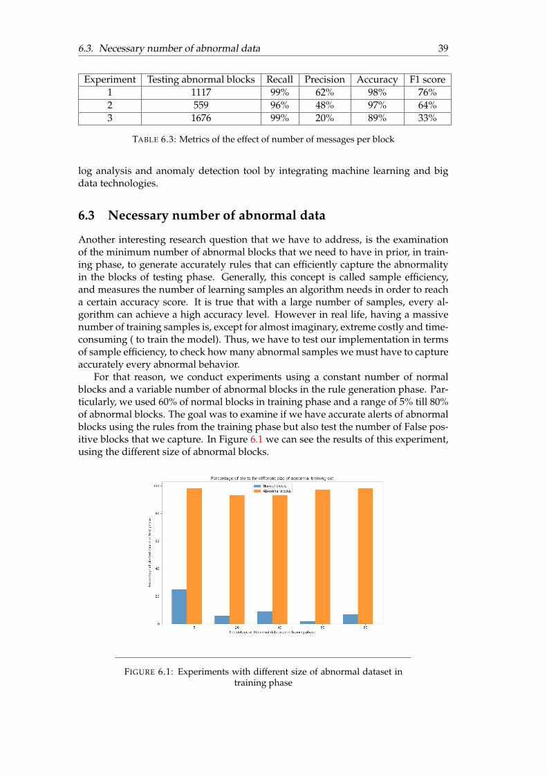
6.3. Necessary number of abnormal data 39

Experiment Testing abnormal blocks Recall Precision Accuracy F1 score1 1117 99% 62% 98% 76%2 559 96% 48% 97% 64%3 1676 99% 20% 89% 33%

TABLE 6.3: Metrics of the effect of number of messages per block

log analysis and anomaly detection tool by integrating machine learning and bigdata technologies.

6.3 Necessary number of abnormal data

Another interesting research question that we have to address, is the examinationof the minimum number of abnormal blocks that we need to have in prior, in train-ing phase, to generate accurately rules that can efficiently capture the abnormalityin the blocks of testing phase. Generally, this concept is called sample efficiency,and measures the number of learning samples an algorithm needs in order to reacha certain accuracy score. It is true that with a large number of samples, every al-gorithm can achieve a high accuracy level. However in real life, having a massivenumber of training samples is, except for almost imaginary, extreme costly and time-consuming ( to train the model). Thus, we have to test our implementation in termsof sample efficiency, to check how many abnormal samples we must have to captureaccurately every abnormal behavior.

For that reason, we conduct experiments using a constant number of normalblocks and a variable number of abnormal blocks in the rule generation phase. Par-ticularly, we used 60% of normal blocks in training phase and a range of 5% till 80%of abnormal blocks. The goal was to examine if we have accurate alerts of abnormalblocks using the rules from the training phase but also test the number of False pos-itive blocks that we capture. In Figure 6.1 we can see the results of this experiment,using the different size of abnormal blocks.

FIGURE 6.1: Experiments with different size of abnormal dataset intraining phase


From Figure 6.1 we can see that despite the size of training set of abnormalblocks, 5%, 20%, 40%, 60% and 80%, we manage to have alerts on around 96% -98% of all abnormal blocks in the testing phase. Thus, with this result we can pro-pose that using even a small number of abnormal block to generate rules, we canefficiently capture all the necessary abnormality for finding future abnormal data.Another useful insight from the above experiment is the number of incorrect alertsof normal blocks. Specifically we can see that using 5% of abnormal blocks, we gotalerts on 25% of all normal blocks in test phase. As the size of abnormal blocks intraining is increasing, the percentage of normal alerted blocks is decreasing, whichmeans less false positive results. However, since a common case in real life is tohave lots of normal data but really few abnormal ones, we can conclude that evenwith small number of abnormal data, we can efficiently use our framework to detectfuture abnormality. However, the size of the available abnormal data will affect thefalse positive rate, which is the faulty alerted blocks in our case, but not in an extentto be restrictive for the use of our framework

6.4 Experiment to improve Precision

In the previous section we saw that our tool has a great performance in detectinganomalies, which is proven by the achieved Recall. However there is a clear issuewith the levels of Precision and F1 score which are quite low. The reason for theselow values is that, despite the detection of almost all abnormal blocks, we categorizealso a significant number of normal blocks as abnormal. These results are associatedwith the rules generation. More specifically, in the rule generation phase, we endup with some rules that represent the normal behavior. The reason is that we havea really large number of normal data and probably the support factor that we usedin generating normal rules and comparing with the abnormal is not the most ap-propriate. Thus despite the fact the we have ended up with a support value of 0.01based on the Bayesian optimization, we will conduct experiments of using a lowersupport value during the normal rule generation. The results of these experimentsare presented in Tables 6.4 and 6.5.

Support value TP FP TN FN0.009 1057 546 40902 600.007 1058 305 41143 590.005 1084 25 41423 330.001 1082 5 41443 35

TABLE 6.4: Results using different support factor on normal rule gen-eration

Support value Recall Precision F1 score0.009 94.6% 66% 77.7%0.007 94.7% 77.6% 85.3%0.005 97% 97.7% 97.3%0.001 96.8% 99.5% 98.1%

TABLE 6.5: Metrics using different support factor on normal rule gen-eration

6.5. Algorithm computational complexity analysis 41

As we can see, by lowering the support value in normal rule generation, wehave less False Positive results and consequently we have a great improvement onthe Precision and F1 score value. Furthermore, we can also argue that there is asmall degradation in the performance of the tool in terms of Recall. However thisdegradation is not that significant, thus we can conclude that using a support factorof 0.01 in abnormal rules generation and a value of 0.001 in the normal rules, we havethe best results for our tool. Although the good performance in these experiments,there is a possibility of overfitting the system since with such a small support value,we actually capture all the possible normal patterns, which however need furtherinvestigation to determine it’s impact in the generalization of the algorithm.

6.5 Algorithm computational complexity analysis

In this last experiment we will try to measure the computational complexity of ourtechnique and to examine which factors have the greatest impact. Based on our im-plementation, each message (or sequence of messages) are tested with every rulein order to find a match. Thus, theoretically the complexity of our algorithm isO(message ⇤ rules). However, we want to examine in what extend each of thesetwo factors affect the performance of our system.

For that reason we will measure the runtime of the algorithm by tuning these twofactors. Specifically we will measure the time when the first data enters the Flinkjob until the last data passing through the Flink operation for the pattern matching.The two factors that we want to investigate is the number of rules that we will testfor matching and the size of the testing data that we have. For that reason we usedifferent number of rules from 5 to 50. For the size of the testing data we use differentsplit percentage for train and test. The result of this experiment is presented in Figure6.2 as well as the number of log messages in each testing percentage in Table 6.6.

FIGURE 6.2: Runtime experiments

To begin with interpreting the above results, we have to present the number oflog data in each of the three cases.


Testing Percentage Number of log messages40% 1.024.29420% 576.85310% 243.075

TABLE 6.6: Number of log messages per test set

In the first case, when using the 40% of the dataset for testing, we can see that,especially after using 30 rules, the runtime is really high. More importantly, in thatcase, after using more than 40 rules, the Flink job was crashing due to memory is-sues. On the other hand, using a smaller number of log data, we can see that theruntime is quite low, independently of the number of rules that we examine. Thus,we can conclude that our framework is being influenced, in term of runtime, mainlyfrom the size of the input data and not from the number of rules. In real life, proba-bly we will not have that high number of testing data in a short period of time, butalso not limited resources, so our anomaly detection framework is working quiteefficiently also it terms of runtime execution.

6.6 Comparison with similar works

From all the above experiments we can see that our work has really promising re-sults in term of anomaly detection in distributed system’s log. However, it is crucialto evaluate our results by comparing with the results of other works that were fo-cused on the same data. To begin with, a master thesis work exists [19], where theyconduct experiments with unsupervised techniques as well as a deep learning ap-proach, such as LSTM, to detect anomalies in same HDFS logs. The best results theyachieve was a Recall and Precision score of 88% and 89% respectively. Another workthat used the same data comes from [12], in which they used again deep learningtechniques. Their Precision and Recall score was 95% and 96% respectively. Finally,Xu et al. [51], who are the people that generated HDFS dataset, achieve a Recall rateof 100% and a Precision of around 87%, using data mining and statistical learningmethods.

Thus, we can conclude that our system outperforms the majority of the alreadyexisting method of detecting anomalies on the same dataset, opening a totally newfield of using rule mine and complex event processing for anomaly detection in logs.Furthermore, we can argue that our approach is also simpler that the aforemen-tioned, such as Deep learning techniques. This is a great advantage since it needsless time to train the model that conduct the anomaly detection.

43

Chapter 7

Scaling out anomaly detection inthe cloud

7.1 Pipeline

One great challenge of this thesis is to create a framework that will be entirely hostedinto the cloud. Thus, the decision was to build the anomaly detection frameworkand all the necessary tools inside a cluster in the cloud. After the examination of allthe available tools that exist and can support our work, we decide to build our toolusing 4 well-known tools, Kubernetes, FluentD, Kafka and Flink.

Beginning with Kubernetes, the idea was to create a Kubernetes cluster and hostall the remaining tools there as pods. Also since we are in the era of Micro-servicesand lots of applications are split in smaller services, one possibility is to host all theservices inside the cluster. As a results, it will be easier to gather the logs of thedifferent services and conduct an anomaly detection in logs using our tool. FluentDis a really important tool since it can collect all the logs of the different applicationto a centralize space. In our case however, since we will have one application thatgenerate logs, FluentD will be configured to read data only from that source. Alsoanother advantage of FluentD is that it has a well integration with Kafka, which isour next tool that we used.

Using Kafka, we have a great tool for passing all the necessary data and spread-ing them to our desire directions. Thus, during Kafka installation, we have createdtwo Kafka topics, one to publish the log data and one to publish the anomaly de-tection results. Last but not least, we choose to use Flink as a way to handling thestreaming log data. Also, since one research question of this thesis is to automate thecomplex event processing engine and Flink contains a really powerful CEP engine,it was inevitable that we will use this tool. Combining Flink’s power in streamingprocessing and the complex event processing engine, we can unlock a whole newfield with lots of possibilities in the anomaly detection of any system’s logs.

As we said before, one goal is to package all the tools into one framework insidea cluster. In Figure7.1 we can see how the architecture of the tool looks like. Also itis crucial to explain the data flow in the system. From Figure 7.1 we can understandhow the data flow, but in the next paragraph we provide a brief explanation of thatflow and the decision behind that.

7.1.1 Data flow

As presented in Figure 7.1, the entire framework is hosted in a Kubernetes cluster.The application that is responsive for the rules generation is deployed as a pod andits results are saved to a file into the Persistent Volume [30] of the cluster. The scriptthat plays the role of log generator, which is also deployed as a pod in the cluster,

44 Chapter 7. Scaling out anomaly detection in the cloud

FIGURE 7.1: Framework Structure

read the entire raw file of HDFS logs and it prints the log messages line by lineas real logs. Fluentd, which is our log collector in the cluster, read the logs of theaforementioned pod and publish each line to a Kafka topic. Then Flink is connectedwith Kafka in order to read the logs from the Kafka topic as streaming data. Inparallel, Flink reads the file with the rules that was saved in the storage of the clusterin order to create the necessary patterns for the complex event processing engine.Finally, the results, which in our case are the blocks that have been predicted asabnormal, are published back to another Kafka topic.

7.2 Large scale configuration

In this section we will describe the main technologies that we use in the implementa-tion of the thesis project, including their purpose and why we chosen them instead ofother similar frameworks. Furthermore, we will describe the configuration parame-ters of each tool in order to have a fully working anomaly detection framework.

7.2.1 Scaling system

In order to scale out our system we have decided to host every different service andtool into a cluster. For that reason we choose Kubernetes to be the host system forour anomaly detection tool.

7.2. Large scale configuration 45

Definition

Kubernetes is a portable, extensible open-source platform for managing container-ized workloads and services, that facilitates both declarative configuration and au-tomation. It has a large, rapidly growing ecosystem. Kubernetes services, support,and tools are widely available. Google open-sourced the Kubernetes project in 2014.Kubernetes builds upon a decade and a half of experience that Google has with run-ning production workloads at scale, combined with best-of-breed ideas and prac-tices from the community [22].

FIGURE 7.2: Kubernetes

Kubernetes will serve us as the main tool. All other tools that will be used, willbe deployed inside the Kubernetes cluster. In such way it is easier to monitor all thetools that we will use and also we can be sure that we will achieve the concept ofMicro-service. Also, it has to be mentioned that the Kubernetes cluster was hostedon Microsoft Azure cloud. The reason for using the Azure Kubernetes Services wasthat it is a really easy and efficiently way to create a Kubernetes cluster in the cloud,without considering updating and maintenance of all cluster components such asthe nodes.

Configuration

As we have mentioned before, our entire framework will be hosted in a Kubernetescluster running on Azure. The most important configuration of the cluster is thatwe have to define a Persistent Storage [30] space for our framework. Thus we needto define a Persistent Volume and a Persistent volume claim. The value of the former isto provide to the cluster a solid storage space on which our tool can save differentnecessary files, such as the file that contains the rules, as we will describe later. Thelatter gives access to a user to use this Persistent Volume storage. Also since weare working with streaming and maybe infinite data, it is really important to havea solid storage to store these data instead to spread them to all Kubernetes clusterwith the risk of facing memory and storage issues.

7.2.2 Containers

In order to deploy application to Kubernetes cluster, we have to create containers ofeach different tool that we want to deploy. Containers are really famous nowadaysbecause you can have an application and all necessary dependencies and librariestogether into one image. For that reason, we decide to containerize all our tools withthe help of Docker. Docker [11] is a tool that was designed to deploy and run appli-cation using containers. Using containers, as we mentioned above, you can combineyour application and the necessary libraries and dependencies into one package in


order to run it in almost any environment. Thus, with Docker you can dockerizeevery kind of application into image and deploy it to Kubernetes cluster, which isour goal.

FIGURE 7.3: Docker

Docker contains some really useful concepts that have to be mentioned here.

• Docker Images: Docker is similar to a virtual machine image, however themain difference is that images in docker share the Linux kernel with the hostmachine. Thus Docker has better performance and it is more lightweight thana general virtual machine.

• Dockerfile: Dockerfiles are scripts that define how to build the docker image,just like Makefiles. In a Dockerfile you can specify the necessary dependenciesand library that your image needs and environmental variables in order toinstall your application properly.

In this work, for the Python applications that we created, we had to build ourown images and thus we created our specific Dockerfiles. For the tools that weused, such as Flink and Kafka, we used already build images provided by differentcontributors.

7.2.3 Log collector

Since all services will be hosted into a Kubernetes cluster, it is necessary to find anappropriate tool that can collect all the important logs that we want. Thus we chooseto use FluentD as log collector.

Definition

Fluentd is an open source data collector, which lets you unify the data collection andconsumption for a better use and understanding of data. Fluentd tries to structuredata in JSON format, as much as possible. This allows Fluentd to unify all facets ofprocessing log data: collecting, filtering, buffering and outputting logs across multi-ple sources and destinations [43].

Thus we used Fluentd in order to collect all logs from the Kubernetes cluster andship them to our storage tool (Kafka). The reason for choosing Fluentd instead ofother log shippers like Logstash, was that it is really fast and it needs less resourcesin contrast to other tools. Also it pre-process the logs in order to transform theminto JSON format which help us to analyze them easier. Furthermore it has lots ofinput and output plugins so it can be connected easy with other tools. Finally it candeployed as Daemonset(will be analyzed later) on Kubernetes to collect the logs ofall application and services.


FIGURE 7.4: FluentD

Configuration

The reason we choose FluentD to be part of the framework is that it can provide uswith the important mechanism of collecting all the logs from the systems and trans-mit them to the desire sources. To deploy FluentD to the Kubernetes cluster, we haveto take into consideration different configuration parameters and some different de-ployments.

To begin with, the first action is to deploy a Service Account [31] for the FluentD.The purpose of this is to to give access to all FluentD pods to the Kubernetes API.Next we have to define a ClusterRole for the tool to have grant access to all resources(pods and nodes) and a ClusterRoleBinding [28] which will bind the ClusterRole ofFluentd as well as the Service Account that we defined in the previous step. Follow-ing that, the next step is to deploy the FluentD to Kubernetes as a DaemonSet[29].The purpose of deploying the tool as a Daemonset is to ensure that when a new nodeis added to the cluster, then automatically a new FluentD pod will be also createdin order to collect all the logs for the new added Node. Finally the last action is tocreate a configuration file for the FluentD with all the necessary configurations. Forinstance we have to restrict from which pod the tool will read the logs. Since weonly have one specific pod that will produce logs in our case, it is crucial to definethe parameter for FluentD to read data only from that pod. In any other case, sincewe have deployed the tool as a Daemonset, we will have logs from all the pods in thecluster, something that in our case will make our framework a way more complex.Another important parameter is to define the Kafka Broker on which it will publishthe logs that it collects and the memory usage in order to collect and publish the logsto the desired Kafka topic.

7.2.4 Message sink

Then it is crucial to find a tool which will collect the logs, as well as to send themto other tools. Thus we need a tool to play the role of mediator on a data flow. Forthat reason we decided to use the well known tool, called Kafka, which is also easilyintegrated with other tools such as FluentD.

Definition

Apache Kafka is an open source project for handling real-time data streams. Ini-tially is was developed by LinkedIn who then open sourced it as an Apache projectin 2011. It is a distributed messaging system providing fast, highly scalable and re-dundant messaging through a pub-sub model. Kafka’s distributed design gives it


several advantages. First, Kafka allows a large number of permanent or ad-hoc con-sumers. Second, Kafka is highly available and resilient to node failures supportingautomatic recovery. In real world data systems, these characteristics make Kafka anideal fit for communication and integration between components of large scale datasystems [2].

The basic architecture of Kafka consists of topics, producers, consumers and bro-kers. All Kafka messages are organized into topics. If you wish to send a messageyou send it to a specific topic and if you wish to read a message you read it from aspecific topic. A consumer pulls messages off of a Kafka topic while producers pushmessages into a Kafka topic. Lastly, Kafka, as a distributed system, runs in a cluster.Each node in the cluster is called a Kafka broker.

FIGURE 7.5: Apache Kafka

In our project, Kafka serves the role of a storage tool in which we store all thestreams of logs that we want to analyze, publishing them to a specific topic, beforebeing processed by other tools like Flink.

Configuration

Kafka is one of the most important tools in our framework since it is actually thechannel where the data actual flows. Thus, it is important to have an actual workingand stable Kafka cluster inside Kubernetes cluster. So except for Kafka, we have todeploy Zookeeper as well, to maintain configuration information, naming, provid-ing distributed synchronization and group services to coordinate Kafka nodes.

Zookeeper

Zookeeper [55] is a top-level software developed by Apache that acts as a central-ized service and is used to maintain naming and configuration data and to provideflexible and robust synchronization within distributed systems. Zookeeper keepstrack on status of the Kafka cluster nodes and it also keeps track of Kafka topics andpartitions.


FIGURE 7.6: Zookeeper

Configuration

Initial we have to create a Service to resolve the domain name to an internal ClusterIP. This IP uses Kubernetes internal proxy to load balance calls to any Pods foundfrom the configured selector. Also we create a Headless service to return all the IPsof Kafka pods based on the above Service. The last step is to deploy Zookeeperas a Statefulset. The value of Statefulsets on Kubernetes is that it offer stable andunique network identifiers, persistent storage, ordered deployments, scaling, dele-tion, termination and automated rolling updates. Alongside with the Statefulset, wedeployed also a PodDisruptionBudget to keep the Zookeeper service stable duringKubernetes administrative events such as draining a node or updating Pods. Thenumber of zookeeper pods that we used is three in order to have a stable deploy-ment without memory issues for our case.

Kafka

The Deployment of Kafka contains the same steps as Zookeeper’s. Thus, in the endwe have a cluster of three Kafka brokers. However, in the configuration file of Kafkawe set also the two topics that we will use. In first topic we will publish the logdata that we will send then to Flink and in the other topic we will publish the alerts(abnormal blocks) as being resulted from the Flink’s complex event processing Job.

7.2.5 Streaming processing

The final tool that is needed is a streaming processing tool to handle the streaminglogs. Also we want a tool that contains a complex event processing engine sincethis is one of our main functions that our anomaly detection tool need. Thus, weuse Flink, which is the best tool for processing streaming data and also contains apowerful complex event processing API.

Definition

Apache Flink [14],[7] is an open source framework for processing streaming data.Its streaming engine, which provide the user with low-latency and high-throughputis written in both Java and Scala. It is the number one tool nowadays for streamingprocessing, taking the place of Spark in the streaming field. Flink contains a variate


of API with Datastream, Dataset and Complex event processing APIs being amongthe most important ones. Except for the APIs, a Flink cluster consist of three types ofprocesses. The first one is the client which is responsible transform the source codeof a program into a dataflow graph. Then, a client submit this graph to the secondprocess, which is the Job manager. The role of Job manager is to coordinates the dis-tributed execution of the graph and defines the Task managers, which will actuallyprocess the data. Task managers are the third crucial component in a Flink cluster.They are responsible for the actual processing and execution of the necessary opera-tion of the program and they report their status and results back to the Job manager.Finally, it has to be mentioned that the aforementioned dataflow graph is a directedacyclic graph (DAG) which consist of data streams and stateful operators.

FIGURE 7.7: Flink

Configuration

Flink is our main stream processing framework and the tool that we want to auto-mate. For the deployment of Flink into the Kubernetes cluster we used the generaldeployment as mention in the tutorial [16]. Specifically we deployed one Job Man-ager and two Task managers, each with 1Gb of Java Heap memory, 8 CPU cores and32Gb physical disk. Also we deployed a service to resolve the domain name to aninternal Cluster IP. Except for these default configurations, lots of parameters haveto be tuned inside the Flink job that we created, which are analyzed in Chapter 5.

7.2.6 Rule generator and log publisher

The program that is responsible for rules generation was Dockerized to an imagewith the help of Docker and then is was deployed as a pod to the cluster. Its config-uration file just gives access to the storage of the cluster to store the resulted rulesto a file. Furthermore, since we do not have a real Hadoop cluster running into thecloud, but only the log data, we had to make a "fake" application to simulate theoperation of Hadoop that produce the logs. Thus we make a simple application thatread the log data from a file and then it just prints them line by line, as a real ap-plication logs. The log publishing program was also Dockerized , without the needfor having access to the storage volume. However the singularity of this applicationcome to the function that read and prints the logs. Since the reading and printing ofa file is a very simple function, due to the high speed of execution, Kafka is unableto read properly all the logs lines, but instead it reads only a part of it. The actualproblem was the way that Kubernetes prints the logs and consequently what logsFluentD collect to transit to Kafka. Due to log file rotation of inner system of Ku-bernetes we have to reduce the speed of printing the data from the python function.Thus we used a time sleep of some millisecond in order to have properly all the datapublished to Kafka topic. Except for that, another configuration of that program was


to print endlessly data after the file is finished. The reason behind that, was a limi-tation between the cooperation of Kafka and Flink. When Flink read streaming datafrom Kafka, is needed, in a periodical time, from Kafka to send a heartbeat to thetask managers of Flink, otherwise the entire Flink job fails. Thus after the end of thelog file we just send every twenty seconds data from the responsible pod to Kafkaand then to Flink. Both programs were implemented using Python programminglanguage. Both programs were implemented using Python programming language.

53

Chapter 8

Discussion and Conclusion

8.1 Discussion

In this work, we managed to create a real-time anomaly detection tool by integratingdata mining technologies along with complex event processing that is deployed inthe cloud. We automate the difficult and time-consuming process of defining rulesin a complex event processing engine with the purpose of receiving alerts on futureanomaly data. Furthermore, the entire framework was build using large scale tech-nologies resulting to a concrete and scalable anomaly detection system. As we havepresented in Chapter 6, we have really promising results. Specifically, we achievea value of Recall around 98% and a Precision around 99%. Furthermore, anothersuccess is the scalability of the system which is hosted inside a Kubernetes clusterand the integration multiple popular big data frameworks. Finally, a strong point ofthis work is the ease deployment of the whole framework into the cloud, somethingreally important for any industry that wants to exploit the capabilities of this work.

Except for our work’s success, at this point, it is crucial to examine if we havemanaged to answer the research questions that we have defined in Chapter 1.

• Can we detect real-time anomalies in system logs in the cloud?: This question wasanswered as the overall outcome of this thesis work. We managed to createa real-time anomaly detection tool and deployed in the cloud using big datatools.

• Can we use rule mining techniques to capture abnormalities in logs?: In Chapter4 we apply rule mining techniques to examine if we can capture abnormal-ity. From the experiments we can verify that we manage to capture abnormalbehavior in logs with 98% accuracy.

• Can we learn rules that represent abnormal behavior?: As an outcome of the previ-ous research question we manage to learn which patterns represent the abnor-mality and thus can be used in next steps of this thesis work.

• What technology can exploit patterns from logs?: The answer to this question isthe Complex Event Processing engine that we used in our tool. We translatethe rules into CEP patterns to rise alerts on abnormal streaming data.

• What is the minimum number of abnormal data during training, in order to accuratecapture future abnormalities?: This question, as we mentioned in Chapter 6, isrelated to the concept of sample efficiency. Specifically it measures the neces-sary training samples a model needs in order to reach a desired accuracy level.Since in real life, but also in our case, it is costly and impossible to have a mas-sive number of abnormal training samples, it is crucial to test the efficiency of

54 Chapter 8. Discussion and Conclusion

our implementation in terms of the required number of data points. In the ex-periments in Chapter 6 we tried to answer this question. Eventually we haveproven with even the 5% of the abnormal data that we have we managed todetect almost all abnormal blocks in test phase. Thus even with small numberof available data, our tool is quite effective.

• On what use case for the industry this work can be applied?: The last question willbe answered in a more abstract way. Since our tool was implemented in thecloud, it is really useful from companies that host their services in the cloud aswell. Furthermore, we used data from a real distributed system that is widelyused by all modern and decent companies. Thus, the system can be appliedas well to data of other distributed systems that companies use. Finally, moreand more software architectures make use of the concept of microservices. Socollected logs form the different services and conduct anomaly detection tofind root cause in case of failure is possible using our system.

8.2 Limitations

Despite its success, this thesis work shares some limitations that have to be men-tioned. Each of the following limitations is related to a different part of the work,such as the implementation part or to a research perspective area.

• Rule generation: For our system to be working, we have first to generate therules and then to feed the Flink job with the streaming data. Thus, in case ofupdating the rules, we have to stop the job and re-run it after the completionof the rule generator. That means that we cannot generate rules on streamingdata, but only on static.

• Memory management: This limitation has been revealed in the runtime experi-ment in Chapter 6. Despite the fact that memory optimization is a subject outof scope of this thesis, with the experiment in Section 6.5, we saw that thereis an issue in memory management. When we have a massive number of logmessages( eg. 1.5 million messages), our framework fails to process all thedata in a small period of time. This issue is highly related to an internal issueof complex event processing of Flink. Since the streaming data pass throughevery rule in the complex event processing engine, without any deletion of oldand examined data, after some time the memory becomes full resulting somememory and runtime problems.

• Number of Rules: A limitation related to the number of rules also exists. Forinstance, from experiments, we figured out that some generated rules are reallysimilar to each other, resulting to an increased number of rules. For example,two possible generated rules are "5 22 5" and "5 22 5 5 5". We can see that thefirst rule is also part of the second. However our system will generate boththese rules, making the system a bit slower since it will examine the streamingdata on both these almost same rules. Thus it is efficient enforce a minimumprefix property on the space of the generated rules in order to solve the issueof similar generated rules.

• Generalization: Lastly, a drawback of our anomaly detection system is that ithas not been tested with another dataset. Since finding a real-time log datasetis quite challenging, we managed to test our system only with the HDFS logs.

8.3. Conclusion and further improvements 55

However with the right pre-processor, the framework can efficiently generalizeto other log data.

8.3 Conclusion and further improvements

To conclude, in this thesis work we investigate the possibility of creating an anomalydetection system for distributed log files. Additionally, we wanted to integrate rulemining technique with complex event processing and deploy the entire system tothe cloud for scalability purposes. In a great extent we managed to achieve all thegoals of this work, developing to a tool with really promising results in the filed ofanomaly detection in system logs. Thus, this system can be applied in different casessuch as root cause analysis of systems or even for predicting future failures beforethey actually happen. Since we can detect a problem before it occurs, it is possibleto do the right actions to prevent the systems from failing. However, as in everyproject, there are some further improvements that can be done in the future. In theprevious section we saw that there are some limitations of this work. It is clear thatimprovement have to be done in order to tackle these aforementioned limitations.All these limitations and the further improvements can fall in two different cate-gories. Specifically, in this work, since it is consisted of algorithmic and engineeringpart, improvements exist in both these fields.

Algorithmic improvements

From algorithmic perspective, one improvement is to examine the effect of onlinerule mining techniques for pattern generation on streaming data instead of the clas-sic static approach that was followed in this work. In that way, it will be possible tocreate rules on the fly and having a system that will continuously learn from newabnormal data without the need of model re-train. Another improvement has tobe done in terms of generalization. First an examination of the effectiveness of thetool in another dataset has to be conducted. Then, if it is possible, to create generalpre-processor for all kind of distributed system log data.

Engineering improvements

Since our system was deployed in the cloud and it consists of different tools thatwork together, there are some improvements that could help anyone who wouldlike to use it in production. For instance, an improvement concern the way the toolis deployed into the cloud. In this work we had to deploy every tool independentlyand the to connect them by creating configuration files. An improvement will be todeploy everything at once using for example the Helm technology of Kubernetes.Finally, an improvement can be in terms of memory management in order to solvethe limitation that we have presented above. Since the memory issue stems from theinternal operation of complex event processing of Flink, the alteration of the enginefalls in the engineering part of the work because the entire code of Flink process hasto be changed.

57

Bibliography

[1] Rakesh Agrawal, Tomasz Imielinski, and Arun Swami. “Mining AssociationRules Between Sets of Items in Large Databases, SIGMOD Conference”. In:vol. 22. June 1993, pp. 207–. DOI: 10.1145/170036.170072.

[2] Apache Kafka. URL: https://kafka.apache.org/intro.

[3] Zachary K Baker and Viktor K Prasanna. “Efficient hardware data mining withthe Apriori algorithm on FPGAs”. In: 13th Annual IEEE Symposium on Field-Programmable Custom Computing Machines (FCCM’05). IEEE. 2005, pp. 3–12.

[4] B Ross Barmish and Constantino M Lagoa. “The uniform distribution: A rig-orous justification for its use in robustness analysis”. In: Mathematics of Control,Signals and Systems 10.3 (1997), pp. 203–222.

[5] James S. Bergstra et al. “Algorithms for Hyper-Parameter Optimization”. In:Advances in Neural Information Processing Systems 24. Ed. by J. Shawe-Taylor etal. Curran Associates, Inc., 2011, pp. 2546–2554. URL: http://papers.nips.cc/paper/4443-algorithms-for-hyper-parameter-optimization.pdf.

[6] D Bhayani. “Identification of security breaches in log records using data min-ing techniques”. In: International Journal of Pure and Applied Mathematics 119(Jan. 2018), pp. 743–756.

[7] Paris Carbone et al. “Apache FlinkTM: Stream and Batch Processing in a SingleEngine”. In: IEEE Data Eng. Bull. 38 (2015), pp. 28–38.

[8] CEP. URL: https://flink.apache.org/news/2016/04/06/cep-monitoring.html.

[9] Nitesh V. Chawla et al. “SMOTE: Synthetic Minority Over-sampling Tech-nique”. In: J. Artif. Int. Res. 16.1 (June 2002), pp. 321–357. ISSN: 1076-9757. URL:http://dl.acm.org/citation.cfm?id=1622407.1622416.

[10] B. Debnath et al. “LogLens: A Real-Time Log Analysis System”. In: 2018 IEEE38th International Conference on Distributed Computing Systems (ICDCS). 2018,pp. 1052–1062. DOI: 10.1109/ICDCS.2018.00105.

[11] Docker. URL: https://www.docker.com/.

[12] Min Du et al. “DeepLog: Anomaly Detection and Diagnosis from System Logsthrough Deep Learning”. In: Oct. 2017, pp. 1285–1298. DOI: 10.1145/3133956.3134015.

[13] “ElasticSearch, “Open-Source Log Storage,”” in: (Aug. 2017). URL: https://www.elastic.co/products/elasticsearch.

[14] Flink. URL: https://flink.apache.org/.

[15] Flink event time. URL: https://ci.apache.org/projects/flink/flink-docs-stable/dev/event_time.html.

[16] Flink k8s. URL: https://ci.apache.org/projects/flink/flink- docs-stable/ops/deployment/kubernetes.html.

https://doi.org/10.1145/170036.170072

https://kafka.apache.org/intro

http://papers.nips.cc/paper/4443-algorithms-for-hyper-parameter-optimization.pdf

http://papers.nips.cc/paper/4443-algorithms-for-hyper-parameter-optimization.pdf

https://flink.apache.org/news/2016/04/06/cep-monitoring.html

https://flink.apache.org/news/2016/04/06/cep-monitoring.html

http://dl.acm.org/citation.cfm?id=1622407.1622416

https://doi.org/10.1109/ICDCS.2018.00105

https://www.docker.com/

https://doi.org/10.1145/3133956.3134015

https://doi.org/10.1145/3133956.3134015

https://www.elastic.co/products/elasticsearch

https://www.elastic.co/products/elasticsearch

https://flink.apache.org/

https://ci.apache.org/projects/flink/flink-docs-stable/dev/event_time.html

https://ci.apache.org/projects/flink/flink-docs-stable/dev/event_time.html

https://ci.apache.org/projects/flink/flink-docs-stable/ops/deployment/kubernetes.html

https://ci.apache.org/projects/flink/flink-docs-stable/ops/deployment/kubernetes.html

58 Bibliography

[17] Flink watermarks. URL: https://ci.apache.org/projects/flink/flink-docs-stable/dev/event_timestamps_watermarks.html.

[18] Stephan Grell and Olivier Nano. “Experimenting with Complex Event Pro-cessing for Large Scale Internet Services Monitoring”. In: (Jan. 2008).

[19] Aarish Grover. “Anomaly Detection for Application Log Data" (2018). Mas-ter’s Projects. 635”. In: DOI: https://doi.org/10.31979/etd.znsb-bw4d. URL:https://scholarworks.sjsu.edu/etd_projects/635.

[20] Hossein Hamooni et al. “LogMine: Fast Pattern Recognition for Log Analyt-ics”. In: CIKM. 2016.

[21] M. A. Hayes and M. A. M. Capretz. “Contextual Anomaly Detection in BigSensor Data”. In: 2014 IEEE International Congress on Big Data. 2014, pp. 64–71.DOI: 10.1109/BigData.Congress.2014.19.

[22] Kelsey Hightower, Brendan Burns, and Joe Beda. Kubernetes: Up and RunningDive into the Future of Infrastructure. 1st. O’Reilly Media, Inc., 2017. ISBN: 1491935677,9781491935675.

[23] Breier Jakub and Jana Branišová. “Anomaly Detection from Log Files UsingData Mining Techniques”. In: Lecture Notes in Electrical Engineering 339 (Jan.2015), pp. 449–457. DOI: 10.1007/978-3-662-46578-3_53.

[24] K. Jayan and A. K. Rajan. “Preprocessor for Complex Event Processing Systemin Network Security”. In: 2014 Fourth International Conference on Advances inComputing and Communications. 2014, pp. 187–189. DOI: 10.1109/ICACC.2014.52.

[25] K. Jayan and A. K. Rajan. “Sys-log classifier for Complex Event Processingsystem in network security”. In: 2014 International Conference on Advances inComputing, Communications and Informatics (ICACCI). 2014, pp. 2031–2035. DOI:10.1109/ICACCI.2014.6968471.

[26] T. Kimura et al. “Proactive failure detection learning generation patterns oflarge-scale network logs”. In: 2015 11th International Conference on Network andService Management (CNSM). 2015, pp. 8–14. DOI: 10.1109/CNSM.2015.7367332.

[27] Ron Kohavi et al. “A study of cross-validation and bootstrap for accuracy es-timation and model selection”. In: Ijcai. Vol. 14. 2. Montreal, Canada. 1995,pp. 1137–1145.

[28] Kubernetes Cluster Role. URL: https : / / kubernetes . io / docs / reference /access-authn-authz/rbac/.

[29] Kubernetes Daemonset. URL: https://kubernetes.io/docs/concepts/workloads/controllers/daemonset/.

[30] Kubernetes Persistent Volume. URL: https://kubernetes.io/docs/concepts/storage/persistent-volumes/.

[31] Kubernetes Service account. URL: https://kubernetes.io/docs/tasks/configure-pod-container/configure-service-account.

[32] Q. J. Lei. “Online monitoring of manufacturing process based on autocep”. In:International Journal of Online Engineering. 2017.

[33] Alessandro Margara, Gianpaolo Cugola, and Giordano Tamburrelli. Towardsautomated rule learning for complex event processing. Tech. rep. 2013.

https://ci.apache.org/projects/flink/flink-docs-stable/dev/event_timestamps_watermarks.html

https://ci.apache.org/projects/flink/flink-docs-stable/dev/event_timestamps_watermarks.html

https://scholarworks.sjsu.edu/etd_projects/635

https://doi.org/10.1109/BigData.Congress.2014.19

https://doi.org/10.1007/978-3-662-46578-3_53

https://doi.org/10.1109/ICACC.2014.52

https://doi.org/10.1109/ICACC.2014.52

https://doi.org/10.1109/ICACCI.2014.6968471

https://doi.org/10.1109/CNSM.2015.7367332

https://kubernetes.io/docs/reference/access-authn-authz/rbac/

https://kubernetes.io/docs/reference/access-authn-authz/rbac/

https://kubernetes.io/docs/concepts/workloads/controllers/daemonset/

https://kubernetes.io/docs/concepts/workloads/controllers/daemonset/

https://kubernetes.io/docs/concepts/storage/persistent-volumes/

https://kubernetes.io/docs/concepts/storage/persistent-volumes/

https://kubernetes.io/docs/tasks/configure-pod-container/configure-service-account

https://kubernetes.io/docs/tasks/configure-pod-container/configure-service-account

Bibliography 59

[34] L. Mariani and F. Pastore. “Automated Identification of Failure Causes in Sys-tem Logs”. In: 2008 19th International Symposium on Software Reliability Engi-neering (ISSRE). 2008, pp. 117–126. DOI: 10.1109/ISSRE.2008.48.

[35] Nijat Mehdiyev et al. “Determination of Rule Patterns in Complex Event Pro-cessing Using Machine Learning Techniques”. In: Procedia Computer Science 61(Dec. 2015), pp. 395–401. DOI: 10.1016/j.procs.2015.09.168.

[36] Alexandra Moraru. “COMPLEX EVENT PROCESSING AND DATA MININGFOR SMART CITIES”. In: 2012.

[37] Raef Mousheimish, Yehia Taher, and Karine Zeitouni. “Automatic Learning ofPredictive CEP Rules: Bridging the Gap Between Data Mining and ComplexEvent Processing”. In: Proceedings of the 11th ACM International Conference onDistributed and Event-based Systems. DEBS ’17. Barcelona, Spain: ACM, 2017,pp. 158–169. ISBN: 978-1-4503-5065-5. DOI: 10.1145/3093742.3093917. URL:http://doi.acm.org/10.1145/3093742.3093917.

[38] C. Mutschler and M. Philippsen. “Learning event detection rules with noisehidden Markov models”. In: 2012 NASA/ESA Conference on Adaptive Hardwareand Systems (AHS). 2012, pp. 159–166. DOI: 10.1109/AHS.2012.6268645.

[39] Jian Pei et al. “Prefixspan: Mining sequential patterns efficiently by prefix-projected pattern growth”. In: Proceedings 17th international conference on dataengineering. IEEE. 2001, pp. 215–224.

[40] Erick Petersen, Marco To De Leon, and Stephane Maag. “An online learningbased approach for CEP rule generation”. In: Nov. 2016, pp. 1–6. DOI: 10.1109/LATINCOM.2016.7811563.

[41] Erick Petersen et al. “An Unsupervised Rule Generation Approach for OnlineComplex Event Processing”. In: Nov. 2018, pp. 1–8. DOI: 10.1109/NCA.2018.8548210.

[42] Clifton Phua et al. A Comprehensive Survey of Data Mining-based Fraud DetectionResearch (Bibliography). May 2013.

[43] Fluentd Project. Fluentd | Open Source Data Collector. URL: https : / / www .fluentd.org/.

[44] Ariel Rabkin and Randy Katz. “Chukwa: A system for reliable large-scale logcollection”. In: Proceedings of the 24th International Conference on Large Installa-tion System Administration (Jan. 2010).

[45] Scala. URL: https://www.scala-lang.org/.

[46] Konstantin Shvachko et al. “The hadoop distributed file system.” In: MSST.Vol. 10. 2010, pp. 1–10.

[47] Jasper Snoek, Hugo Larochelle, and Ryan P Adams. “Practical Bayesian Op-timization of Machine Learning Algorithms”. In: Advances in Neural Informa-tion Processing Systems 25. Ed. by F. Pereira et al. Curran Associates, Inc., 2012,pp. 2951–2959. URL: http : / / papers . nips . cc / paper / 4522 - practical -bayesian-optimization-of-machine-learning-algorithms.pdf.

[48] “Splunk, “Turn Machine Data Into Answers”. In: (Aug. 2017). URL: https://www.splunk.com.

[49] J. Wei et al. “Analysis farm: A cloud-based scalable aggregation and queryplatform for network log analysis”. In: 2011 International Conference on Cloudand Service Computing. 2011, pp. 354–359. DOI: 10.1109/CSC.2011.6138547.

https://doi.org/10.1109/ISSRE.2008.48

https://doi.org/10.1016/j.procs.2015.09.168

https://doi.org/10.1145/3093742.3093917

http://doi.acm.org/10.1145/3093742.3093917

https://doi.org/10.1109/AHS.2012.6268645

https://doi.org/10.1109/LATINCOM.2016.7811563

https://doi.org/10.1109/LATINCOM.2016.7811563

https://doi.org/10.1109/NCA.2018.8548210

https://doi.org/10.1109/NCA.2018.8548210

https://www.fluentd.org/

https://www.fluentd.org/

https://www.scala-lang.org/

http://papers.nips.cc/paper/4522-practical-bayesian-optimization-of-machine-learning-algorithms.pdf

http://papers.nips.cc/paper/4522-practical-bayesian-optimization-of-machine-learning-algorithms.pdf

https://www.splunk.com

https://www.splunk.com

https://doi.org/10.1109/CSC.2011.6138547

60 Bibliography

[50] Wei Xu et al. “Detecting Large-scale System Problems by Mining Console Logs”.In: Proceedings of the ACM SIGOPS 22Nd Symposium on Operating Systems Prin-ciples. SOSP ’09. Big Sky, Montana, USA: ACM, 2009, pp. 117–132. ISBN: 978-1-60558-752-3. DOI: 10.1145/1629575.1629587. URL: http://doi.acm.org/10.1145/1629575.1629587.

[51] Wei Xu et al. “Online System Problem Detection by Mining Patterns of Con-sole Logs”. In: Proceedings of the 2009 Ninth IEEE International Conference onData Mining. ICDM ’09. Washington, DC, USA: IEEE Computer Society, 2009,pp. 588–597. ISBN: 978-0-7695-3895-2. DOI: 10 . 1109 / ICDM . 2009 . 19. URL:https://doi.org/10.1109/ICDM.2009.19.

[52] Chengqi Zhang and Shichao Zhang. Association rule mining: models and algo-rithms. Springer-Verlag, 2002.

[53] Qiankun Zhao and Sourav S Bhowmick. “Sequential pattern mining: A sur-vey”. In: ITechnical Report CAIS Nayang Technological University Singapore 1 (2003),p. 26.

[54] Qiankun Zhao and Sourav S Bhowmick. “Association Rule Mining: A Sur-vey”. In: Jan. 2003.

[55] Zookeeper. URL: https://zookeeper.apache.org/.

https://doi.org/10.1145/1629575.1629587

http://doi.acm.org/10.1145/1629575.1629587

http://doi.acm.org/10.1145/1629575.1629587

https://doi.org/10.1109/ICDM.2009.19

https://doi.org/10.1109/ICDM.2009.19

https://zookeeper.apache.org/

Real-time anomaly detection in logs using rule mining and ...

Documents

Transcript of Real-time anomaly detection in logs using rule mining and ...