NBER WORKING PAPER SERIES

REAL OPTIONS, TAXES AND FINANCIAL LEVERAGE

Stewart C. MyersJames A. Read, Jr.

Working Paper 18148http://www.nber.org/papers/w18148

NATIONAL BUREAU OF ECONOMIC RESEARCH1050 Massachusetts Avenue

Cambridge, MA 02138June 2012

We thank William Shore and Wei Dou for research assistance and several helpful comments. Theviews expressed herein are those of the authors and do not necessarily reflect the views of the NationalBureau of Economic Research.

NBER working papers are circulated for discussion and comment purposes. They have not been peer-reviewed or been subject to the review by the NBER Board of Directors that accompanies officialNBER publications.

© 2012 by Stewart C. Myers and James A. Read, Jr.. All rights reserved. Short sections of text, notto exceed two paragraphs, may be quoted without explicit permission provided that full credit, including© notice, is given to the source.

Real Options, Taxes and Financial LeverageStewart C. Myers and James A. Read, Jr.NBER Working Paper No. 18148June 2012JEL No. G31,G32

ABSTRACT

We show how the value of a real option depends on corporate income taxes and the option’s “debtcapacity,” defined as the amount of debt supported or displaced by the option. The value of the underlyingasset must be an adjusted present value (APV). The risk-free rate of interest must be after-tax. Debtcapacity depends on the APV and target debt ratio for the underlying asset, on the option delta andon the amount of risk-free borrowing or lending that would be needed for replication. The target debtratio for a real call option is almost always negative. Observed debt ratios for growth firms that followthe tradeoff theory of capital structure will be lower than target ratios for assets in place. Our resultscan rationalize some empirical financing patterns that seem inconsistent with the tradeoff theory, butrigorous tests of the theory for growth firms seem nearly impossible.

Stewart C. MyersMassachusetts Institute of TechnologySloan School of ManagementE62-62077 Massachusetts AvenueCambridge, MA 02142and NBERscmyers@mit.edu

James A. Read, Jr.The Brattle Group44 Brattle StreetCambridge, MA 02138Jamie.Read@brattle.com

2

1. INTRODUCTION

Consider a tax-paying corporation with an option to invest in a real asset. The

option is to be valued as a derivative by the risk-neutral method, that is, by calculating the

payoffs to the option as if the expected rate of return on the underlying asset is equal to

the risk-free rate and then discounting. What is the discount rate? It is the risk-free rate,

of course, but pre-tax or after-tax?

Accurate valuation of real options depends on the correct answer to this question.

The answer also has important implications for debt policy and tests of the tradeoff

theory of capital structure. If the tradeoff theory is correct and risk and debt capacity of

assets in place are constant, then a firm with no growth options will have a constant target

debt ratio, and will adjust back towards that ratio when its actual ratio is off-target. But a

firm with valuable growth options will not operate at a constant debt ratio, and will

usually move to a lower debt ratio when the values of its assets and options increase. As

we will show, some empirical results that seem inconsistent with the tradeoff theory may

actually be explained by the dynamics of target debt ratios for growth options.

Back to the beginning question on taxes and discounting: Taxes are important, not

just because corporations pay them, but also because interest tax shields are valuable.

Project NPVs are typically calculated by discounting at a tax-adjusted rate, for example at

an after-tax weighted average cost of capital (WACC). Tax-adjusted discount rates

depend on the debt supported by a project’s cash flows as well as on the cash flows’

business risk. To value a real option, we must therefore determine the amount of debt

supported or displaced by the option.

Black-Scholes (1973) and Merton (1973) demonstrated that a call option can be

replicated by delta (δ) units of the underlying risky asset less a specific amount of riskless

borrowing. We can always express the value of a real option as the net value of these

two components of a replicating position. The first component (δ units of the underlying)

is perfectly correlated with the underlying asset and should have the same proportional

debt capacity. The second component (borrowing) should displace ordinary debt on a

dollar-for-dollar basis. Thus the debt capacity of a real option will depend on the value

and debt capacity of the underlying asset and the amount of implicit borrowing. The

3

interest on the debt in a replicating portfolio is not tax-deductible, however. Thus there is

a tax cost when implicit option debt displaces ordinary borrowing.

We show how to calculate real option values using a risk-and-debt-neutral method.

The method is most easily implemented by the following two steps.

1. Calculate the APV of the underlying real asset, including the present value of interest

tax shields on debt supported by the asset. Use this APV as the value of the

underlying asset. (The APV is often calculated in one step by discounting cash flows

at an after-tax WACC).)

2. Calculate the all-equity after-tax payoffs to the real option as if the expected rate of

return on the underlying asset were equal to the after-tax risk-free rate. Then

discount the payoffs to the option at the after-tax rate.

The second step operates in an after-tax risk-neutral setting, where the risk-neutral rate is

set so that the expected rate of return on the underlying asset equals the after-tax risk-free

rate.

Our method assumes that capital structure is continuously rebalanced to maintain

a debt ratio equal to the target for corporate assets, including the corporation’s real

options. This assumption can be only approximately correct, but it follows common

practice. For example, discounting at an after-tax weighted average cost of capital

(WACC) requires that future debt ratios stay constant. The assumption also follows from

the tradeoff theory of capital structure. If the theory is correct, the firm will always be on

or moving back towards the target.

Preview of Valuation Results

Consider a European option to purchase a real asset at date 1. The exercise price

is a fixed amount X. The real asset is worth PV0 at date 0. Assume for simplicity that it

generates no cash flows between dates 0 and 1. Its cash flows after date 1 are net of

corporate taxes that would be paid by an all-equity firm.

4

Standard practice would value this option by the risk-neutral method, discounting

at the pre-tax risk-free rate r. Suppose this standard valuation has been done properly.

We can write the call value as:

CDcall 0PVPV ,

where δ is the option delta and DC is the implicit option leverage, that is, the amount of

debt that would be needed to replicate the option.

This valuation procedure does not consider how ownership of the real option

affects a corporation’s debt capacity and interest tax shields. The debt capacity of the

option depends on the two terms given above. The first term δPV0 is positive and

proportional to PV0. This term supports debt. The second term DC displaces regular

borrowing, and the implicit interest on DC is not tax-deductible. When option leverage

substitutes for explicit leverage, interest tax shields are lost.

Therefore we must convert both terms to APVs that account for taxes and

leverage:

,1APVAPVAPV 0 rDcall C (1)

where APV0 is the APV of the underlying real asset and rDC 1APV is the APV of

the option leverage.

We write the second APV term as a function of rDC 1 , because this APV

calculation discounts both the principal and implicit interest for DC . The discount rate is

the after-tax risk-free rate. Thus this APV calculation grosses up DC by the factor

Tr

r

11

1, where T is the marginal corporate tax rate. We derive APV formulas in the

next section.

Now suppose we redo the option valuation in a risk-neutral setting where the risk-

free rate is defined after-tax. That is, the risk-neutral drift term is Tr 1 . The asset

value PV0 is not affected, because the drift rate and the discount rate “cancel” when

5

specified consistently. But now the correct APV(call) is calculated automatically, with

no need for a tax gross-up.

This valuation logic can be applied generally. Consider a European call option

with a fixed exercise price X, written on an asset worth PV0 now. The asset will generate

no cash flows or dividends prior to option expiration τ periods in the future. The Black-

Scholes-Merton value would normally be calculated as:

rXdNdNcall 1PVPV 201

We adapt the Black-Scholes-Merton formula for leverage and taxes by substituting APV0

for PV0 and the after-tax rate Tr 1 for the pre-tax rate r. The APV of the call is then:

TrXdNdNcall 11APV APV 201 (2)

where 1d and 2d are now the arguments of the normal distribution function calculated

using APV0 for the underlying asset and the after-tax risk-free rate.

Preview of Implications for Capital Structure

The tradeoff theory assumes that the firm has a target debt ratio, which is

determined by the risk and other attributes of the firm’s assets, and that the actual debt

ratio equals the target on average and reverts to the target over time. Many tests of the

tradeoff theory take its predictions as qualitative. We can be more precise.

Suppose that the static-tradeoff theory holds exactly. Then the implicit debt in

real (call) options must displace explicit borrowing. Of course only explicit borrowing

shows up in observed debt ratios. Several empirical implications follow:

1. The target debt ratio for a real call option is always less than the target debt ratio

for the underlying asset. Therefore firms with valuable real options will have

lower market debt ratios.

6

2. The net debt capacity of real call options is in most cases negative. Therefore

valuable call options will in most cases lead to lower borrowing relative to assets

in place. If book values are adequate proxies for assets in place, then firms with

more valuable growth options will usually operate at lower book debt ratios.

3. The net debt capacity of real options depends on the value of the underlying asset,

the exercise price of the options, and other option-pricing inputs, including

volatility and interest rates. Therefore the firm’s target book and market debt

ratios cannot be stable over time, even if the firm’s portfolio of assets in place and

real options is held constant.

4. Growth options should not increase the equity standard deviation or beta. Growth

options are of course more volatile than assets in place, but debt policy cancels

out any increase.

Of course these predictions assume that growth options account for a material part of

the market value of the firm. This is not true for all firms, but is true for many.

Prior Research

The interplay of taxes, financing and the cost of capital has been well-covered in

the finance literature on the valuation of real assets. Key papers include Myers (1974),

which introduces the APV method, Miles and Ezzell (1980), Taggart (1991) and Ruback

(1986).1 Taxes and financing are also important in practice. For example, they affect

valuations when cash flows are discounted at an after-tax weighted average cost of

capital (WACC) and in APV calculations. The PV of interest tax shields motivates

corporate borrowing in the tradeoff theory of capital structure. But as far as we know, the

effects of corporate leverage and taxes on the valuation of real options have never been

addressed.

The pre-tax risk-free rate is used to value real options in practice. Discount rates

are not adjusted for taxes and leverage. For example, Dixit and Pindyck “largely ignore

taxes” (1994, p. 55). They and Copeland and Antikarov (2001) do not adjust the discount

1 For a summary, see Brealey, Myers and Allen (2010, Chapter 19). See also Ruback (2002).

7

rate for taxes. Brennan and Schwartz’s (1985) real-options analysis of natural resource

investments values cash flows after taxes but uses a pre-tax risk-free rate. All of the

examples in McDonald’s (2006) practice-oriented survey discount at the pre-tax rate.

Brealey, Myers and Allen (2010) cover taxes and leverage in detail when explaining

WACC and APV, but then use the pre-tax risk-free rate in their chapter on real options.

Ruback (1986) explained why the after-tax rate Tr 1 should be used to value

risk-free cash flows. See also Brealey, Myers and Allen (2011, pp. 498-501). Intuition

suggests that the after-tax rate should also be used to discount certainty-equivalent option

payoffs. We show that the intuition is correct when valuing implicit option leverage.

Modigliani and Miller (MM) (1963) derive the tax- and leverage-adjusted

discount rate ri* = ri (1 – λT), where ri is the opportunity cost of capital for assets in risk

class i and λ is the target debt ratio for the firm.2 Nowadays ri would be defined as an

unlevered cost of capital, likely derived from the capital asset pricing model (CAPM).

Myers, Dill and Bautista (1976) derive the discount rate for financial leases as

r = rD(1 – λT), where rD is the pre-tax cost of debt and λ is the fraction of debt supported

or displaced by the lease. These discount rates are useful for calculating APVs in some

circumstances, but are not adapted to value real options. But we will derive a similar

discount-rate formula for valuing certainty equivalent cash flows from real assets.

The after-tax weighted average cost of capital (WACC) is widely used in

corporate finance. It is useful for valuing real assets but not for valuing real options.

Application of a constant WACC to discount multi-period cash flows assumes not only

that the systematic risk of the cash flows is constant, but also that debt capacity is

constant fraction of value. This assumption is wrong for real options.

We are not the first to consider how real options could affect capital structure

choices. Some empirical results have been attributed in a qualitative way to the presence

of growth options. For example, growth firms with high market-to-book ratios tend to

use less debt, which makes sense if growth options increase market values but have little

2 Myers (1974) shows that the MM formula works only for level perpetuities and fixed borrowing. The correct formula for finite-lived projects with expected cash flows that vary over time is in Miles and Ezzell (1980).

8

or no debt capacity. See Barclay, Smith and Watts (1995) for a summary of this view of

the evidence.

Barclay, Morellec and Smith (2006) present an agency model in which growth

options have negative debt capacity and present empirical results indicating that firms

with growth options tend to operate at low book debt ratios. We agree with these authors

that growth options usually have negative debt capacity, but our modeling approach is

different from theirs. They present an agency model in which debt constrains managers’

impulse to overinvest. We start with standard option valuation methods – no agency

issues – and simply derive the implications of the tradeoff theory when real options are

important.

We also note a related literature on how growth options affect the risk of levered

common equity. Gomez and Smidt (2010) and Jacquier, Titman and Yalcin (2010) are

recent examples. The latter article shows that equity betas are more closely linked to the

implicit leverage in growth options than to explicit borrowing.3 Again we agree, but our

approach is different, because we use the tools of option valuation and corporate finance

in order to derive specific predictions about capital structure if the tradeoff theory is

correct.

The logic of tax- and leverage-adjusted valuation of real options is introduced by

binomial examples in Section 2. Section 3 generalizes the binomial analysis, introduces

the modified Black-Scholes-Merton formula and calculates examples of errors when real

options are valued without adjusting for taxes and leverage. Section 4 summarizes the

implications of real options for optimal capital structure and tests of the static tradeoff

theory.

2. EXAMPLES

The logic of our APV approach to option valuation is best introduced in one-

period binomial examples. We will concentrate on calls, although the same logic applies

to puts. We assume a pre-tax risk-free rate of 6%. For simplicity we also assume that the

3 Jacquier, Titman and Yalcin (2010) refer to option leverage as “operating leverage.”

9

corporation can borrow or lend at 6% pre-tax. The opportunity cost of capital is 10%.

The marginal corporate tax rate is T = 35%.

APV of the Underlying Asset

Start with the value of the underlying real asset; the growth option will enter in a

moment. Assume that the asset generates a single expected cash payoff of V1 = 110 after

corporate taxes at t = 1. There are no intermediate cash flows between t = 0 and t = 1.

Discounting at the opportunity cost of capital gives a present value V0 = 110/1.10 = 100.

The asset’s payoff can also be expressed as a certainty-equivalent payoff of CEQ(V1) =

106. Discounting at the 6% risk-free rate gives the same V0 = 100.

This valuation assumes all-equity financing and does not include the value of

interest tax shields on the debt supported by the asset. Assume that the firm’s target debt

ratio for assets in place is λ = 50%, expressed as a fraction of APV.

1010495.1

106

35.05.0106.01

106

11

CEQ

1

APV

1

CEQAPV 111

1

Tλr

V

r

VrT

r

VV

APV(V1) includes the value of one period’s interest tax shields on debt of 50.5. The tax

shields are worth 1.0. Note that the certainty-equivalent discount rate is Tr 1 . The

term T1 adjusts for leverage and taxes, as in the MM cost of capital formula. Note

too that the relationship between the PV and the tax-adjusted APV is

Tr

rVV

11

1PVAPV 11 .

We will work with certainty-equivalent cash flows in this paper to give a clearer

comparison of discount rates for real assets and real options. But the APV of 101 could

have been calculated by discounting the expected payoff of 110 at an after-tax weighted

(3)

10

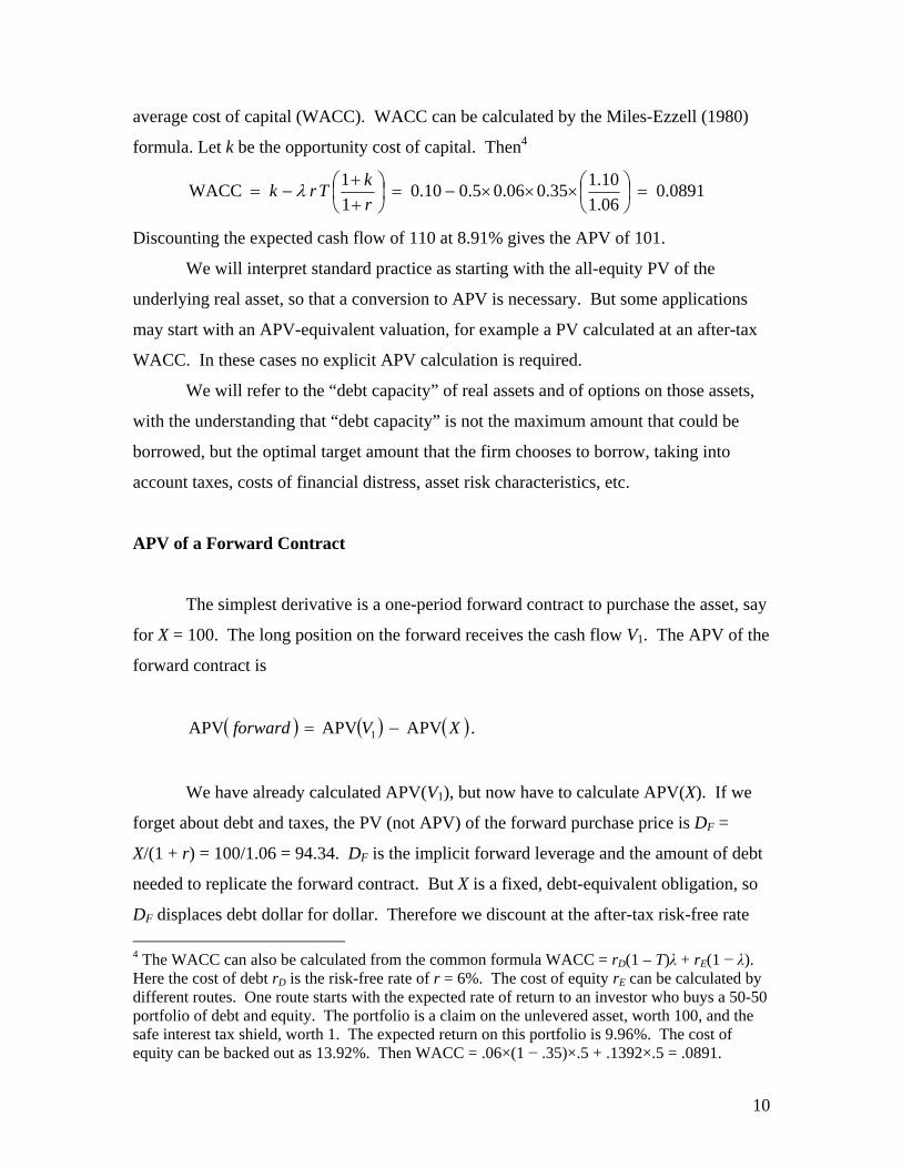
average cost of capital (WACC). WACC can be calculated by the Miles-Ezzell (1980)

formula. Let k be the opportunity cost of capital. Then4

0891.006.1

10.135.006.05.010.0

1

1WACC

r

kTrk

Discounting the expected cash flow of 110 at 8.91% gives the APV of 101.

We will interpret standard practice as starting with the all-equity PV of the

underlying real asset, so that a conversion to APV is necessary. But some applications

may start with an APV-equivalent valuation, for example a PV calculated at an after-tax

WACC. In these cases no explicit APV calculation is required.

We will refer to the “debt capacity” of real assets and of options on those assets,

with the understanding that “debt capacity” is not the maximum amount that could be

borrowed, but the optimal target amount that the firm chooses to borrow, taking into

account taxes, costs of financial distress, asset risk characteristics, etc.

APV of a Forward Contract

The simplest derivative is a one-period forward contract to purchase the asset, say

for X = 100. The long position on the forward receives the cash flow V1. The APV of the

forward contract is

XVforward APVAPVAPV 1 .

We have already calculated APV(V1), but now have to calculate APV(X). If we

forget about debt and taxes, the PV (not APV) of the forward purchase price is DF =

X/(1 + r) = 100/1.06 = 94.34. DF is the implicit forward leverage and the amount of debt

needed to replicate the forward contract. But X is a fixed, debt-equivalent obligation, so

DF displaces debt dollar for dollar. Therefore we discount at the after-tax risk-free rate

4 The WACC can also be calculated from the common formula WACC = rD(1 – T)λ + rE(1 − λ). Here the cost of debt rD is the risk-free rate of r = 6%. The cost of equity rE can be calculated by different routes. One route starts with the expected rate of return to an investor who buys a 50-50 portfolio of debt and equity. The portfolio is a claim on the unlevered asset, worth 100, and the safe interest tax shield, worth 1. The expected return on this portfolio is 9.96%. The cost of equity can be backed out as 13.92%. Then WACC = .06×(1 − .35)×.5 + .1392×.5 = .0891.

11

.06(1 − .35) = .039, which gives APV(X) = 100/1.039 = 96.25. (This APV calculation

follows from Eq. (3) when λ = 100%.)

The APV of the forward contract is 101 – 96.25 = +4.75. Notice that calculating

the contract’s APV requires two discount rates, Tr 1 ) for the underlying asset and

Tr 1 for the forward purchase price. Notice also that using the after-tax rate to

discount the forward price grosses up DF by the factor Tr

r

11

1.

The debt capacity of the forward contract is negative. APV(V1) supports debt of

50.50. APV(X) displaces explicit borrowing of 96.25. The net debt capacity is – 45.75.

A firm holding the forward purchase contract would borrow 45.75 less against its other

assets and appear to operate at an excessively conservative debt ratio.5

APV of a Real Call Option

Now consider a one-period call option for the same real asset with an exercise

price of X = 100. We start with standard valuation practice, using a one-period, pre-tax

binomial event tree with rate of return outcomes of +25% (the “up” branch) and –20%

(the “down” branch). The risk-neutral probabilities of the up and down branches are p =

.5778 and 1 – p = .4222, so that the expected rate of return is equal to the pre-tax risk-free

rate.

Asset Call

p = .5778 125 (+1.0605) + 25

V0 = 100 (+1)

APV(V1) = 101

1 – p = .4222 80 (+1.0605) 0

5 Marking the forward contract to its market value of 4.75 and putting this net value on the asset side of the balance sheet does not solve this problem. The firm would still appear to have unused debt capacity from its assets in place. Fully revealing accounting would split the forward contract, showing APV(V1) on the left side of the balance sheet and APV(X) as an explicit debt-equivalent liability on the right.

12

Interest tax shields on debt supported by the asset are split out and shown in parentheses.

The tax shields are determined by borrowing at t = 0 and do not depend on the up or

down outcome at t = 1. The payoffs to the call do not yet take account of interest tax

shields.

The PV (not yet APV) of the call is (.5778×25)/1.06 = 13.63. We can break out

this value as the difference between two values, just as for the forward contract. The two

values are δ = .5556 units of the asset and implicit debt of DC = 41.93.

63.1393.4156.55callPV 0 CDV .

These two values show the replicating portfolio for the call.6 The first term is δ units of

the real asset. The second term DC is the PV of a future fixed payment of 41.93 plus

interest of rDC = .06×41.93 = 2.52. We now have to calculate the APV of each term.

The first term δV0 has the exactly same risk as the asset in place and therefore the

same fractional debt capacity of λ = 50%. Thus the APV of the first term is δAPV(V1) =

.5556×101 = 56.11.7 The second term DC displaces debt dollar for dollar. Its APV must

take account of the tax shields lost on the debt that it displaces. We therefore discount

the future payment of rDC 1 = 41.93 + 2.52 = 44.45 at the after-tax risk-free rate of

3.9%. So rDC 1APV = 44.45/1.039 = 42.78. The APV of the call is:

rDVcall C 1APVAPVAPV 1 = 56.11 – 42.78 = 13.33

As for the forward contract, there are two tax-adjusted discount rates. APV(V1)

can be valued by discounting the certainty equivalent of V1 at Tr 1 . rDC 1APV

is valued by discounting DC, plus interest on DC, at the after-tax risk-free rate Tr 1 .

6 Most real options cannot be explicitly replicated and hedged, but that does not change valuation principles. See Brealey, Myers and Allen (2011, pp. 569-570). 7 In this example the option delta does not depend on whether V1 or APV(V1) is used for the underlying real asset.

13

The calculation for rDC 1APV grosses up the option leverage DC by a factor of

Tr

r

11

1.

The debt capacity of the call is negative. The first term supports debt of

λδAPV(V1) = .5×.5556×101 = 28.06. The option’s implicit leverage displaces debt of

42.78. Net debt capacity is 28.06 – 42.78 = − 14.72. Real call options usually displace

explicit debt, although they can have positive debt capacity if they are far enough in the

money.8

Suppose the firm has one asset in place worth APV = 101 and a real call option to

buy one more. If the firm’s debt is on target, its market-value balance sheet (showing

explicit debt only) is:

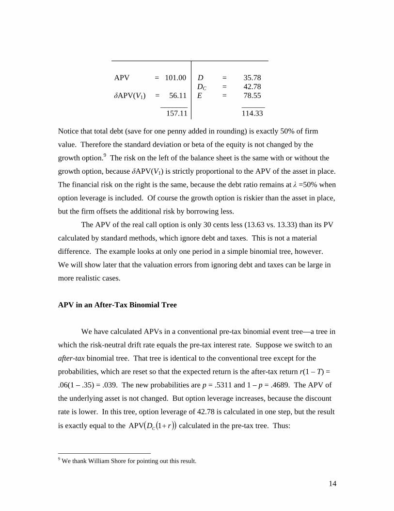
APV = 101.00 D = 35.78

APV(call) = 13.33 E = 78.55 _______ ______

114.33 114.33

The asset in place has debt capacity of 50.50, but the firm only borrows 35.78, because

the call’s debt capacity is –14.72. The market debt ratio would be recorded as only

35.78/114.33 =.31, far below the target debt ratio of 50% against the APV of assets in

place. The firm would appear to operate at a conservatively low debt ratio. In fact it is at

its debt target. It is borrowing the same 50% fraction of the APV of the asset in place and

of δAPV(V1), the option’s position in an identical asset by way of the call. But it is also

reducing borrowing dollar for dollar to compensate for the APV of the leverage in the

call.

We can also write the balance sheet making showing the option leverage

explicitly:

8 Change our example so that X = 25 rather than 100. Now δ = 1 and δλAPV(V1) = 50.50. The APV of the option debt is 25.51. The net contribution to debt capacity is 50.50 – 25.51 = +24.99.

14

APV = 101.00 D = 35.78 DC = 42.78

δAPV(V1) = 56.11 E = 78.55 _______ ______

157.11 114.33 Notice that total debt (save for one penny added in rounding) is exactly 50% of firm

value. Therefore the standard deviation or beta of the equity is not changed by the

growth option.9 The risk on the left of the balance sheet is the same with or without the

growth option, because δAPV(V1) is strictly proportional to the APV of the asset in place.

The financial risk on the right is the same, because the debt ratio remains at λ =50% when

option leverage is included. Of course the growth option is riskier than the asset in place,

but the firm offsets the additional risk by borrowing less.

The APV of the real call option is only 30 cents less (13.63 vs. 13.33) than its PV

calculated by standard methods, which ignore debt and taxes. This is not a material

difference. The example looks at only one period in a simple binomial tree, however.

We will show later that the valuation errors from ignoring debt and taxes can be large in

more realistic cases.

APV in an After-Tax Binomial Tree

We have calculated APVs in a conventional pre-tax binomial event tree—a tree in

which the risk-neutral drift rate equals the pre-tax interest rate. Suppose we switch to an

after-tax binomial tree. That tree is identical to the conventional tree except for the

probabilities, which are reset so that the expected return is the after-tax return r(1 – T) =

.06(1 – .35) = .039. The new probabilities are p = .5311 and 1 – p = .4689. The APV of

the underlying asset is not changed. But option leverage increases, because the discount

rate is lower. In this tree, option leverage of 42.78 is calculated in one step, but the result

is exactly equal to the rDC 1APV calculated in the pre-tax tree. Thus:

9 We thank William Shore for pointing out this result.

15

33.1378.4211.561APVAPVAPV 1 rDVcall C

Switching from the pre-tax to the after-tax tree increases option leverage by the factor

Tr

r

11

1, the same as the gross-up required in the pre-tax tree. Therefore we can

bypass the conversion of DC to rDC 1APV and just value real-option leverage in an

after-tax risk-free setup. Details are in the next section.

3. BINOMIAL AND BLACK-SCHOLES-MERTON FORMULAS FOR REAL

OPTIONS

Now we generalize to a real call option on a longer-lived asset. We present

valuation formulas for valuing a European call on the asset for each time interval in a

binomial event tree. The formulas converge to Black-Scholes-Merton as calendar time is

divided into smaller intervals and the number of intervals becomes very large.

Assume that the asset generates a known constant cash-flow yield y that is

proportional to end-of-period APV.10 The payoff at date t + 1 from purchasing the asset

at date t is APVt+1(1 + y) + λrTAPVt. APVt+1 captures the present value at t + 1 of all

subsequent cash flows and associated interest tax shields.

The asset can be valued recursively, discounting expected payoffs at a tax- and

leverage-adjusted discount rate. If the expected payoffs are certainty equivalents, as in

Eq. (3), APV0 is:

Tr

y

r

Try

11

1APVCEQ

1

APV1APVCEQAPV

1

010

10 A constant cash-flow yield implies that the asset is a growing, declining or constant perpetuity. The cash flow yield for a finite-lived asset would have to increase as the asset approached its final date.

16

Once APV0 is calculated we can proceed to value a call on the asset. We start as

before with a conventional, pre-tax binomial tree with up and down steps u and d = 1/u.

We use APV as the value of the underlying asset.

Asset Call

p [uAPV0 (1+y) Cu − rTDC

+ λrTAPV0]

APV0

(1 – p) [dAPV0 (1+y) Cd − rTDC

+ λrTAPV0]

The option payoffs in this tree include two terms. The first terms Cu and Cd are

standard. For example, if the option matures in the next period, Cu = Max(uAPV0 – X, 0)

and Cd = Max(dAPV0 – X, 0). (The option does not get the cash flow yield yAPV0 or the

interest tax shield λrTAPV0 on debt supported by the underlying real asset.) The second

term rTDC captures the interest tax shields lost because of debt displaced by the option’s

implicit leverage.

The equations for option replication in the pre-tax tree are:

Cu − rTDC = δuAPV0 − DC(1 + r) and Cd − rTDC = δdAPV0 − DC(1 + r),

Cu = δuAPV0 − DC(1 + r(1 − T)) and Cd = δdAPV0 − DC(1 + r(1 − T)).

Eq. (4) implies that the fractional debt capacity of a real call option is always less than for

the underlying asset. The debt capacity would be the same (λ) but for option leverage DC,

which enters as a negative term in Eq. (4).

The lost tax shields rTDC are the same in the up and down states, so the formula

for the option delta is 0APVdu

CC du

. Given δ, the amount of debt displaced is:

0 0APV APV

1 1 1 1

u d

C

u C d CD

r T r T

(4)

(5)

17

Eq. (5) for DC discounts at the after-tax rate r(1 – T). The standard formula, which

ignores interest tax shields on displaced debt, would discount at the pre-tax rate r. Thus

Eq. (5) grosses up option leverage by the factor (1+r)/(1+r(1 – T)).

Of course the gross-up is not needed in an after-tax binomial tree, where the

expected risk-neutral rate of return on the asset is Tr 1 . The APV of option leverage

is generated automatically in the after-tax tree, with no required explicit adjustment for

interest tax shields lost because of displaced debt. The after-tax tree is identical to the

conventional tree, except for the pseudo probabilities, which depend on the after-tax risk-

free rate. The probability of the “up” branch is:

du

dy

Tr

p

111

Moving from the pre-tax to after-tax tree does not change the state variable APV0(1 + y).

The amount of debt in the replicating portfolio changes, because of the gross-up for lost

interest tax shields on ordinary debt displaced by option leverage.

Volatility of APV in discrete time

We used APV0 as the state variable in the binomial event tree. APV0 includes

the interest tax shield λrTAPV0, which is fixed by borrowing at t = 0 and does not depend

on the outcome at t = 1. This tax shield does not affect the payoffs to the call or the

dollar spread between up and down payoffs to the real asset, but it does reduce the risk of

the next payoff to the real asset. Therefore the shield could affect volatility and the choice

of u and d, the rate of return outcomes in the tree. Thus we pause to consider what

determines volatility when APV is used as the state variable in a discrete-time binomial

setup.

The call does not receive next period’s interest tax shield or the cash flow yield

yAPV1. The call’s value depends only on APV1, which has the same volatility as the

18

unlevered asset value V1. Thus the up and down moves u and d = 1/u should be based on

the volatility of APV1.11

The only safe interest tax shield is the first one, λrTAPV0. Later tax shields share

all the risks of future cash flows and APVs. For example, the value at date t = 1 of the

tax shield at date t = 2 is proportional to the realized V1 and APV1. It is proportional

because the firm is assumed to rebalance its capital structure at date t = 1 and borrow the

fraction λ of the realized outcome APV1. Viewed from date t = 0, the interest tax shield

for t = 2 has exactly the same risk as APV1 or the unlevered payoff V1. So do the interest

tax shields for t = 3, 4, … . When the firm rebalances its capital structure every period,

the tax shields have the same risk as future cash flows and unlevered asset values.

The volatility of APV0 is different from the volatility of the unlevered value V0

because we are working in discrete time. The difference disappears in continuous time.

Continuous time would, strictly speaking, require continuous rebalancing to the firm’s

target debt ratio.

Our APV analysis assumes that firms rebalance their capital structures exactly to

target, either continuously or at the start of each discrete period. This assumption is of

course a stretch. Standard DCF valuation practice assumes for simplicity that firms do

rebalance, however. For example, discounting at the after-tax WACC assumes that the

firm rebalances to keep its market-value debt ratio constant.12 In this paper we accept

this standard assumption and work out its implications for valuing real options.

Valuing puts

Corporations also hold real put options, that is, options to abandon existing assets.

Puts are valued in the same way as calls, except that puts support debt, not displace it.

Thus we distinguish DP, the debt supported by a put’s negative leverage, from DC, the

11 The cash flow yield is proportional to APV1 and does not affect percentage volatility. 12 The APV method does not require rebalancing every period. It can incorporate fixed debt repayment schedules or debt policies that adjust with lags to target debt capacity. The assumption of prompt rebalancing could also be relaxed for APVs of real options. We do not consider such extensions here, however.

19

debt displaced by the option leverage in a call. The replication equations for a put in the

pre-tax binomial tree are:

Cu + rTDP = (δ − 1)uAPV0 + DP(1 + r) and Cd + rTDP = (δ − 1)dAPV0 + DP(1 + r)

Option leverage DP now has a positive sign, because a put is replicated by a short position

in the underlying asset plus lending. The put-option delta is δ − 1, where δ is the call-

option delta. Thus

Cu = (δ − 1)uAPV0+ DP(1 + r(1 − T)) and Cd = (δ − 1)dAPV0 + DP(1 + r(1 − T)).

The amount of lending required to replicate the put is:

0 0( 1) APV ( 1) APV

1 1 1 1

u d

C

u C d CD

r T r T

Notice that DP is calculated by discounting at the after-tax risk-free rate. The discounting

is automatic in the after-tax binomial tree.

The fractional debt capacity of a real put option is never negative and always

greater than for the underlying asset. This follows from put-option replication, which

requires APV(put) = (δ – 1)APV(V1) + DP, where DP is given by Eq. (7). APV(put) is

non-negative, so DP ≥ (δ – 1)APV(V1). The debt displaced by the short position in the

underlying asset is less than the short position, assuming that the underlying asset is risky

and λ < 1. The put’s debt capacity λ(δ – 1)APV(V1) + DP must therefore be positive. This

debt capacity can approach zero when the put is far out of the money, however.

A Modified Black-Scholes-Merton Formula

Cox, Ross and Rubinstein (1979) showed that in the continuous-time limit, as the

length of the time interval approaches zero and the return parameters r, u and d are

rescaled accordingly, their binomial option pricing formula converges to the Black-

(6)

(7)

20

Scholes-Merton option pricing formula. The convergence proof does not depend on the

nature of the underlying asset (here an APV) or on the definition of the risk-free rate

(here the after-tax rate Tr 1 ).13 Therefore, we can modify the Black-Scholes-Merton

formula to take account of taxes and leverage by (1) substituting the APV of the

underlying asset for the PV and (2) substituting the after-tax risk-free rate for the pre-tax

rate.14 Suppose the underlying asset generates all-equity cash flows at a known rate y in

proportion to its market value. If τ denotes the time remaining to expiration, the APV of

a call is:

TrXdNyAPVdN

XdNVdNcall

111

APVAPVAPV

201

21

2210

1

1ln11lnln

yTr

XAPV

d

12 dd

APV0 is the spot value of the stream of cash flows and associated interest tax shields

generated by the underlying real asset. If the asset generates income before date τ (y > 0),

the APV of the underlying delivered immediately will be greater than APV(Vτ), which is

a deferred claim. This is accounted for by “discounting” at the cash-flow yield rate y.

The Black-Scholes-Merton formula for the value of a real put option is:

13 In a multi-period problem, the composition of the replicating portfolio changes as time elapses and the price of the underlying asset evolves. The multi-period binomial option pricing formula was obtained by imagining a dynamic trading program under which the replicating portfolio is revised at the start of each time interval, so that its payoffs at the end of the time interval again replicate the option payoffs. (In the continuous-time market setting of Black-Scholes-Merton, the dynamic trading program requires continuous portfolio revisions.) Our modified option valuation formula thus reflects an additional implicit transaction at the end of each time interval: corporate borrowing is revised to maintain a target debt ratio in market value terms. 14 Merton (1973) presents the formula for the value of an option on the common stock of a firm that follows a proportional dividend policy.

21

yAPVdNTrXdN

VdNXdNput

111

APVAPVAPV

012

12

The drift term in the modified valuation formulas is the after-tax interest rate

adjusted for payouts. Thus, real options are valued as if the APV of the underlying real

asset is expected to appreciate at the after-tax risk-free rate. One might therefore call the

modified formula “risk-and-debt-neutral valuation”. Thus whether one applies an

analytical formula (such as the modified Black-Scholes-Merton formula), simulation

methods, or numerical approximation procedures, one can work with the APV of the

underlying asset and use an after-tax risk-neutral drift rate (equal to the after-tax risk-free

rate adjusted for payouts).

Notice that the target debt ratio λ does not appear in the valuation formulas.

Thus, the value of a real option does not depend directly on the debt capacity of the

underlying asset, just as the value of an option does not depend directly on the expected

rate of return on the underlying asset. Debt capacity and expected rate of return influence

option values only insofar as they affect the adjusted present value of the underlying.

Option Debt

European calls and puts are equivalent to simple combinations of digital

options—a call (put) option is equivalent to the combination of a short (long) cash-or-

nothing option and a long (short) asset-or-nothing option, both with the same strike price

and time to expiration as the call (put). The debt capacity of a real option is equivalent to

a weighted combination of the same digital components, where the weight on the asset-

or-nothing option is equal to the debt capacity of the underlying asset and the weight on

the cash-or-nothing option is equal to one. Therefore, the debt capacities of real

European-type calls and puts can be calculated using the modified Black-Scholes-Merton

formulas with one further change: the APV of the underlying asset is weighted by its

debt capacity λ. If we let B denote debt capacity, the debt capacities of calls and puts are

given by the following formulas:

22

TrXdNyAPVdNcall 111B 201

yAPVdNTrXdNput 111B 012

Figure 1 is a pair of graphs of option debt in relation to the adjusted present value

of the underlying asset. The options have a strike price of 100 and a time to expiration of

one year. There are three cases: the debt capacity of the underlying asset is 0%, 25%, or

50%. Panel A gives the results for calls, Panel B for puts. Option debt is always less than

or equal to zero for calls if the underlying asset has no debt capacity. Option debt for

calls can be positive if the underlying asset has positive debt capacity and the option is

very deep in the money. Option debt is always greater than or equal to zero for puts.

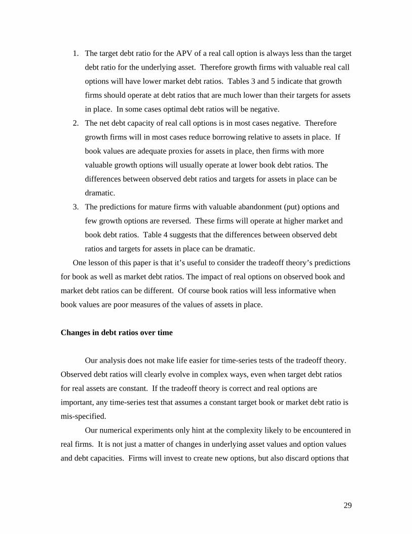
The relationship between option debt and the value of the underlying asset is

further illuminated by Figures 2 and 3, which are graphs of the option debt deltas and

gammas. (The deltas and gammas are the first and second derivatives, respectively, of

option debt with respect to the value of the underlying asset.) Notice that the option debt

deltas can be well in excess of one in absolute value. Also, the deltas for calls on assets

with debt capacity change sign when they are deep in the money. Notice too that the debt

gammas change sign as the options shift from out-of-the-money states to in-the-money

states. Thus, while the relationship between the value of an option and the value of the

underlying asset is rich, the relationship between option debt capacity and the value of

the underlying is even richer.

Examples

The modified Black-Scholes-Merton formula will tell us whether the valuation

errors from ignoring taxes and the debt capacity of real options are important. Table 1

reports the values of real call options with exercise prices of 100. The underlying asset

values (APV) range from 40 to 200. The options are European, with maturities of 1, 3 or

5 years. The tax rate is 35%. Panel A assumes a pre-tax risk-free interest rate of 6%, a

volatility of 20% and a cash flow yield of 10%. Panels B, C and D, respectively, show

results for a 30% volatility, a 9% interest rate and a 0% cash flow yield.

23

Each entry in Table 1 gives the correct option value, taking account of the

option’s debt capacity and the interest tax shields lost because of debt displaced by the

option, and below it the absolute (dollar) and percentage errors from not adjusting for

taxes and leverage. Take for example a 5-year at-the-money option in panel A. The

option is worth 5.01 using the modified Black-Scholes-Merton formula. Valuing the

option by the conventional method – that is, Black-Scholes-Merton with a pre-tax interest

rate – would value the option at 6.79, an overvaluation of 1.78 or 36%.

Table 1 shows that real call options are always overvalued by the conventional

method. Dollar and percentage errors are material. Percentage errors are larger for

longer maturities and larger for out-of-the-money calls than for in-the-money calls.

Absolute errors are large for in-the-money calls. Dollar and percentage errors are also

greater when the pre-tax interest rate is high (Panel C). This is as expected, since the

chief difference between the standard and modified Black-Scholes-Merton model is use

of an after-tax interest rate.15 The tax adjustment to the interest rate matters more when

interest rates are high.

Table 2 shows values and valuation errors for real put options. Puts are

systematically undervalued by conventional methods. Dollar and percentage errors are

again material. For example, the 5-year at-the-money put option in panel A is worth

25.50 using the modified Black-Scholes-Merton formula. The conventional method

would value the option at 25.50, a valuation error of −6.08 or −24%.

These examples show that ignoring taxes and debt capacity can introduce serious

errors in valuing real options. Of course there will also be cases where the errors are not

material and where conventional practice is an acceptable approximation. We do not see

the point of the approximation, however, since the correct tax- and leverage-adjusted

valuation method is no more complicated or burdensome than the conventional method.

Tables 1 and 2 are restricted to simple European calls and puts with fixed exercise

prices. The real options held by corporations are more complex. Our methods should

generalize from simple to more complex options, however. If we assume that the

15 The other potential difference is use of APV for the underlying asset rather than the asset’s unlevered PV. Whether conventional practice would use APV or PV is not so clear. An asset value calculated by discounting expected cash flows at an after-tax WACC is equivalent to an APV. The same cash flows discounted at an unlevered cost of capital give an estimate of PV.

24

tradeoff theory holds, so that firms have meaningful target debt ratios against assets in

place, then taxes and debt capacity have to be accounted for when valuing real options.

4. EMPIRICAL IMPLICATIONS

Growth options have implicit leverage. Other things equal, the tradeoff theory

must therefore predict lower debt ratios for firms with valuable growth options.

Abandonment (put) options have the opposite effect. Puts increase debt capacity and

should allow the corporation to “lever up.”

We do not endorse the tradeoff theory as generally correct and complete, but it’s

nevertheless useful to work out the theory’s empirical implications when the firm holds

valuable real options. We will not attempt a review of research on capital structure,

which is enormous,16 but will give examples of prior research below.

The tradeoff theory predicts that firms will trade off the tax advantages of

borrowing (interest tax shields) against costs of financial distress. Costs of financial

distress include direct costs of bankruptcy or reorganization and also costs from moral

hazard and agency problems caused by default risk. The tradeoff determines a target

capital structure that maximizes overall firm value.

The tradeoff theory makes two broad predictions. The first is cross-sectional:

observed debt ratios should equal target debt ratios on average. Target debt ratios should

vary depending on the firm’s tax status, the risk or other attributes of its assets (tangible

vs. intangible assets, for example) and on how much value would be lost in financial

distress. The second, time-series prediction is that observed debt ratios will fluctuate, but

adjust back towards target debt ratios over time.

The implicit leverage in real options has immediate implications for cross-

sectional tests. The debt capacity of real call options is usually negative and always less

than the debt capacity of assets in place. Therefore a firm with valuable growth options

will appear to operate at a too-conservative debt ratio, compared to the debt capacity of

its assets in place. A mature firm with valuable abandonment (put) options will appear to

16 Review articles include Harris and Raviv (1991), Myers (2003) and Frank and Goyal (2008).

25

operate at an aggressively high debt ratio, because puts contribute debt capacity rather

than displacing it.

Cross-sectional tests of the tradeoff theory

Most cross-sectional tests start with a standard list of variables to “explain”

differences in market or book debt ratios.17 See Rajan and Zingales (1995) and Harris

and Raviv (1991). The most common variables include the following (plus or minus

signs in parentheses show typical effects on debt ratios in the cross section18):

profitability (−); market-to-book ratio (−); tangibility of assets, for example the ratio of

property, plant and equipment to total assets (+), and size, usually the log of total assets

(+). Many other variables have also been tested, but it is useful to start here with these

old standards.

The positive signs for size and tangibility seem reasonable if the tradeoff theory is

correct. Large firms ought to borrow more; they are presumably safer and more likely to

pay taxes. Firms with more tangible assets are less likely to be damaged in financial

distress and should therefore have higher target debt ratios.

The negative signs for profitability and market-to-book are harder to rationalize.

The market-to-book ratio might measure intangible assets in place, which are more liable

to damage in financial distress. But intangibles ought to contribute some positive debt

capacity and at least increase book debt ratios. In fact the market-to-book ratio usually

correlates with lower book as well as market debt ratios. The negative relationship

between profitability and book debt ratios is even harder to explain by the tradeoff

theory. Higher profitability increases debt servicing capacity and also increases taxable

income and the potential value of interest tax shields. Therefore profitable firms should

operate at higher book and market debt ratios, but by and large they don’t.

17 The tradeoff theory is most often interpreted as applying to market-value debt ratios. Book debt ratios are brought in as a check or backup. 18 There are of course exceptions to these “typical effects.” See Appendix C in Antoniou et al. (2008), which tabulates results from dozens of prior research papers that have used these and other variables.

26

These typical results are easier to square with the tradeoff theory when we

recognize real options. Firms with higher market-to-book ratios are more likely to be

firms with more valuable growth options. Our analysis says that such firms will operate

at lower market debt ratios, because growth options have lower debt capacities than

underlying assets in place, and in most cases at lower book debt ratios, because debt

capacity for growth options is usually negative. The negative relationship between

profitability and financial leverage also makes sense if more profitable firms have more

valuable growth options.

Large firms are usually mature firms, which should borrow more if assets in place

account for a greater fraction of their market value than for younger growth firms.

Mature firms are also likely to have valuable abandonment options, which add debt

capacity. Recognizing real put options therefore reinforces the tradeoff theory’s

prediction that large firms should borrow more.

Examples

Table 3 reports debt capacities and debt ratios for firms that have assets in place

worth APV = 100 and real call options to invest 100 in the same assets in year 3. That is,

the firms have options to double in size in year 3. Option values are from Panel A of

Table 1. Thus the tax rate is 35%, the pre-tax risk-free interest rate is 6%, the volatility is

20% and the cash-flow yield rate is 10%. (Versions of Table 3 based on 1- or 5-year

maturities or on other panels of Table 1 tell similar stories.) The top panel of Table 3

assumes a target debt ratio of 25% for assets in place. The bottom panel assumes the

target debt ratio is 50%. The firm is assumed on-target with respect to the debt capacity

of its option as well as its asset in place. The value of the asset in place ranges from 40 to

200.

Table 3 reports negative debt capacity for the call option in all cases. The

negative debt capacity can be double or triple the option’s APV. For example, the at-the-

money option in Panel A is worth 5.62. Its debt capacity is – 15.47.

Also, with one exception, option debt capacity decreases as the option moves

farther in the money. The exception occurs in Panel B when the underlying asset value

27

increases from 150 to 200. In this case option debt capacity increases (becomes less

negative) from −16.54 to −9.39. Debt capacity would continue to increase for still-higher

asset values and eventually turn positive. In the limit, where the ratio of asset value to

exercise price becomes extremely high, the fractional debt capacity of a real call option

approaches λ, the target ratio for the underlying asset.

Table 3 also reports the target debt ratio for the option—the ratio of the option’s

debt capacity to its value—which always increases (becomes less negative) as the option

moves more in the money.

Negative debt capacity means that the option’s implicit leverage displaces

reported leverage. Thus the firm’s market debt ratio in Table 3 is always less than the

25% and 50% target debt ratios for assets in place. In Panel A, the firm operates at a

negative debt ratio when underlying asset value is 150 or higher. The firm is a net lender.

The “book” ratio of debt to assets in place is also less than the target ratios in Table 3.

The book ratio would eventually move above the targets, however, because option debt

capacity turns positive when the option is far enough in the money.

Table 4 reports debt ratios for an aging firm that has assets in place worth APV =

100 and options to abandon (put) its assets for 100 in year 3. Put option values come

from Panel A of Table 2. Format and inputs are the same as in Table 3.

The firm’s market and book debt ratios in Table 4 are always greater than the

25% and 50% target debt ratios for assets in place. The fractional debt capacity of a real

put option is never negative and always greater than for the underlying asset. The put’s

contribution to debt capacity can be double or triple the value of the put itself. For

example, the at-the-money put option in Panel A of Table 4 is worth 19.64. Its debt

capacity is 54.91.

Table 4 probably overstates the debt capacity of real put options, because it

assumes that the exercise price is fixed and risk-free. In practice the proceeds from

abandonment will be uncertain, and will not support debt dollar for dollar. Nevertheless,

debt capacity from puts can help explain why takeovers of mature, cash-cow firms are

often highly levered. For example, LBOs are often diet deals motivated by options to sell

assets and shrink operations. The options increase debt capacity relative to target debt

ratios for assets in place.

28

The results summarized in Tables 3 and 4 were obtained based on the assumption

that the firm holds a single call or put. Essentially the same conclusions follow from

more realistic examples, in which the firm holds a portfolio of calls and/or puts with a

range of expiration dates and exercise prices. Table 5 reports debt ratios for firms

holding a portfolio of fifty call options: ten calls expiring each year from one to five

years and exercise prices ranging in five steps from 50 to 200. Results are reported for

firms with the potential to grow 50%, 100% and 150% over five years. Panels A and B

report debt ratios when the assets in place and underlying assets have a target debt ratio

of 25% and 50%, respectively.

Like the hypothetical firms with a single call options in Table 3, the debt-to-value

ratios for the firms with a portfolio of options in Table 5 are equal or very close to the

target debt ratio when the options are out of the money (underlying value equal to 40),

but decline as the value of the underlying real asset increases. (The cases with 100%

growth potential in Table 5 correspond most closely to the single-option results in Table

3.) The decline in debt-to-value ratios is substantial in all cases—even in the case of 50%

growth potential and a very high target ratio of 50% (Panel B). Debt-to-value ratios are

also not stable—they change when the value of the underlying asset changes.

The ratio of debt to assets in place—the “book” debt ratio—for firms with a

portfolio of options likewise behaves much as the book debt ratio for firms with a single

option.19 The book ratio is close to the target debt ratio when the options are well out of

the money, declines as the value of the underlying assets increases (moving from left to

right in Tables 3 and 5), then becomes flat or even rises as the underlying assets become

very valuable and the options are deep in the money. Also, the book debt ratio is close to

the market debt ratio—the ratio of debt to all assets, including growth options—in most

cases. The exception arises when the target debt ratio for the underlying assets is high

(50%) and the options are deep in the money.

These numerical experiments confirm our cross-sectional predictions for market

and book debt ratios when firms strictly follow the tradeoff theory.

19 In this paper both “book” and “market” debt ratios are calculated based on market values. “Book” debt ratio here means the ratio of debt to the market value of assets in place. We use “book” to distinguish a debt ratio that (like corporate balance sheets) does not reflect the value of growth and abandonment options.

29

1. The target debt ratio for the APV of a real call option is always less than the target

debt ratio for the underlying asset. Therefore growth firms with valuable real call

options will have lower market debt ratios. Tables 3 and 5 indicate that growth

firms should operate at debt ratios that are much lower than their targets for assets

in place. In some cases optimal debt ratios will be negative.

2. The net debt capacity of real call options is in most cases negative. Therefore

growth firms will in most cases reduce borrowing relative to assets in place. If

book values are adequate proxies for assets in place, then firms with more

valuable growth options will usually operate at lower book debt ratios. The

differences between observed debt ratios and targets for assets in place can be

dramatic.

3. The predictions for mature firms with valuable abandonment (put) options and

few growth options are reversed. These firms will operate at higher market and

book debt ratios. Table 4 suggests that the differences between observed debt

ratios and targets for assets in place can be dramatic.

One lesson of this paper is that it’s useful to consider the tradeoff theory’s predictions

for book as well as market debt ratios. The impact of real options on observed book and

market debt ratios can be different. Of course book ratios will less informative when

book values are poor measures of the values of assets in place.

Changes in debt ratios over time

Our analysis does not make life easier for time-series tests of the tradeoff theory.

Observed debt ratios will clearly evolve in complex ways, even when target debt ratios

for real assets are constant. If the tradeoff theory is correct and real options are

important, any time-series test that assumes a constant target book or market debt ratio is

mis-specified.

Our numerical experiments only hint at the complexity likely to be encountered in

real firms. It is not just a matter of changes in underlying asset values and option values

and debt capacities. Firms will invest to create new options, but also discard options that

30

are too far out of the money. Changes in technology and competition will extinguish

options but also create new ones.

But we can say something more definite about how target debt ratios should

change over time in response to random shocks to the firm’s profitability and the value of

its assets in place. We will assume for simplicity that the firm’s portfolio of real options

is held constant.

A positive shock to the value of a firm’s assets in place moves the firm from left

to right in Tables 3, 4 and 5. Notice that the target market debt ratio falls when market

value increases. In other words, the derivative of the target ratio with respect to change

is value is negative, both for growth firms (Tables 3 and 5) and for mature firms with

abandonment options (Table 4).20 For growth firms, the target debt ratio falls even

though the debt capacity of real options increases (or becomes less negative). The reason

is that a positive shock to profitability and asset values increases the proportion of market

value accounted for by the growth options, which always have less debt capacity than

assets in place.

Our numerical experiments are simplified, but it is nevertheless plausible to

predict that firms with valuable real options – abandonment options as well as growth

options – will target a lower market debt ratio when market value goes up. They may

also target a lower book debt ratio – notice how the ratio of debt to assets in place

declines from left to right in Tables 3, 4 and 5.

This negative relationship could explain otherwise difficult puzzles in the

empirical literature on capital structure. Take Welch (2004) as an example. This paper

finds that year-to-year changes in market debt ratios are mostly explained by changes in

stock price, and that net issues of debt and equity do not counteract the effects of stock-

price changes, at least in the short run. If the corporations in Welch’s sample are really

trying to get back to a stable target debt ratio, they are not working very hard at it. In

addition, Welch finds that net issuing activity appears to amplify the effect of stock price

20 Our theory does not require this negative effect for real call options—the derivative turns positive when growth options are far in the money. The negative effect is required for puts, because puts have higher fractional debt capacity than the underlying assets in place. This additional debt capacity dissipates when asset value increases and the put moves out of the money.

31

changes on market debt ratios, at least in the short run. “Over one year, firms respond to

poor [stock price] performance with more debt issuing activity and to good performance

with more equity issuing activity.” (Welch 2004, p. 111.) This behavior is a deep puzzle

if one ignores real options and assumes that the firms are following the tradeoff theory

with a stable target debt ratio. The behavior makes sense if real options are important

and target ratios incorporate the options’ debt capacity. If poor stock price performance

means less valuable growth options and more valuable abandonment options, then target

debt ratios should go up, leading to more debt issuing activity. Good stock price

performance should have the opposite effect.

Predictions about equity risk

Assume the firm has a definite target debt ratio λ for its assets in place, based on

the risks of those assets. If the firm follows the tradeoff theory, then it should rebalance

its capital structure to keep its total leverage – the sum of ordinary borrowing and the

implicit debt in its real options – equal to λ times the sum of the APVs of assets in place

and the sum of the underlying APVs for its real options, each multiplied by its current

option delta. Assume that the assets underlying the real options have the same business

risks as assets in place. Then equity risk (standard deviation or beta) will not depend on

the value of its real options. The real options are of course riskier than the assets in place,

but debt policy compensates.

Equity risk will be strictly constant if asset risk is constant and the firm can adjust

capital structure every period, with no lags or frictions. If capital structure is rebalanced

with lags, as in a target adjustment model, then a positive (negative) shock to profitability

should at first increase (decrease) equity risk. But equity risk will converge gradually to

a target level. This is a testable prediction of the tradeoff theory.

5. CONCLUSIONS

Standard valuation methods take account of project debt capacity and the interest

tax shields on debt supported by the project. “Debt capacity” is not the maximum

32

amount that could be borrowed, but a target amount. The tradeoff theory of capital

structure says that the target should strike a balance (at the margin) between the tax

advantages of borrowing and possible future costs of financial distress.

This paper analyzes growth (call) and abandonment (put) options in this standard

valuation framework. We work with certainty-equivalent cash flows to facilitate

comparison with standard option valuation methods. These standard methods ignore debt

capacity and interest tax shields, however. Certainty-equivalent option payoffs are just

discounted at a pre-tax risk-free rate. This discounting procedure is not correct.

Our results include the following:

1. Valuing assets in place: The correct discount rate for unlevered certainty-

equivalent cash flows is Tr 1 , where r is the pre-tax interest rate, T is the

marginal corporate tax rate and λ is the target debt ratio, expressed as a fraction of

the asset’s adjusted present value (APV).

2. Valuing real options: Use a tax- and leverage-adjusted APV to value of the

underlying real asset. Value real-option payoffs (in a risk-neutral setting) at the

after-tax interest rate Tr 1 . For example, the modified Black-Scholes-Merton

formula uses APV as the asset value and Tr 1 as the interest rate.

3. Real call options have implicit leverage. The fractional debt capacity of a call is

usually negative, and always less than for the underlying asset.

4. The fractional debt capacity of a real put option is always positive and greater

than for the underlying asset.

The following results assume that the firm manages its capital structure according

to the tradeoff theory and that its debt ratio is always on target.

5. The implicit debt in real call options displaces ordinary borrowing. Observed

debt ratios for firms with valuable growth options will be less than target debt

ratios for assets in place. This result may help explain why profitability and

market-to-book ratios are negatively correlated with debt ratios.

6. The implicit lending in real put options supports additional ordinary borrowing.

Debt ratios for firms with valuable abandonment options will be greater than

target debt ratios for assets in place. This result may help explain why large,

mature firms tend to operate at high debt ratios, especially in LBOs.

33

7. When a growth firm’s profitability and value improve, its target market debt ratio

falls. When profitability and value decline, the target ratio increases. (This result

assumes that growth options are valuable, but not too far in the money.)

8. Capital structures should adjust to offset the additional risks of real options,

leaving the standard deviation or beta of equity constant.

Results 5 to 8 may assist our empirical understanding of corporate debt policies.

These empirical predictions clearly require further investigation, however. A detailed

empirical study of options and capital structure is beyond the scope of this paper.

34

REFERENCES

A. Antoniou, Y. Guney and K. Paudyal (2008), “The Determinants of Capital Structure: Capital Market-Oriented versus Bank-Oriented Institutions,” Journal of Financial and Quantitative Analysis 43: 59-92. M. Barclay, E. Morellec and C. Smith (2006), “On the Debt Capacity of Growth Options,” Journal of Business 79, 39-59. M. Barclay, C. Smith and R. Watts (1995), “Determinants of Corporate Leverage and Dividend Policies,” Journal of Applied Corporate Finance 7, 4-19. F. Black and M.S. Scholes (1973), “The Pricing of Options and Corporate Liabilities,” Journal of Political Economy 81, 637-654. R. A. Brealey, S.C. Myers and F. Allen (2011), Principles of Corporate Finance, 10th ed. (McGraw-Hill Irwin). M. J. Brennan and E. S. Schwartz (1985), “Evaluating Natural Resource Investments,” Journal of Business 58: 135-157. T. Copeland and V. Antikarov (2001), Real Options: A Practitioner’s Guide (New York: Texere). J. C. Cox and S. A. Ross (1976), “The Valuation of Options for Alternative Stochastic Processes,” Journal of Financial Economics 3: 145-166. J. C. Cox, S. A. Ross and M. Rubenstein (1979), “Option Pricing: A Simplified Approach,” Journal of Financial Economics 7: 229-263. A.K. Dixit and R.S. Pindyck (1994), Investment under Uncertainty (Princeton, NJ: Princeton University Press). M. Frank and V. Goyal (2008), “Tradeoff and Pecking Order Theories of Debt,” in E. Eckbo, ed., Handbook of Corporate Finance: Empirical Finance, v. 2, North Holland. J. F. Gomez and L. Schmid (2010), “Levered Returns,” Journal of Finance 65, 467-494. M. Harris and A. Raviv (1991), “The Theory of Capital Structure,” Journal of Finance 46: 297-355. E. Jacquier, S. Titman and A. Yalcan (2010), “Predicting Systematic Risk: Implications from Growth Options,” Journal of Empirical Finance 17, 991-1005.

35

R. L. McDonald (2006), “The Role of Real Options in Capital Budgeting: Theory and Practice,” Journal of Applied Corporate Finance 18, 28-39. R. C. Merton (1973), “Theory of Rational Option Pricing,” The Bell Journal of Economics and Management Science 4, 141-183. J. Miles and R. Ezzell (1980), “The Weighted Average Cost of Capital, Perfect Capital Markets, and Project Life: A Clarification,” Journal of Financial and Quantitative Analysis 15, 719-730. M. H. Miller and F. Modigliani (1966), “Some Estimates of the Cost of Capital to the Electric Utility Industry, 1954-57,” American Economic Review 56, 333-391. F. Modigliani and M. H. Miller (1963), “Corporate Income Taxes and the Cost of Capital: A Correction,” American Economic Review 53, 433-443. S.C. Myers (1974), “Interactions of Corporate Financing and Investment Decisions: Implications for Capital Budgeting,” Journal of Finance 29, 11-25. S. C. Myers (2003), “Financing of Corporations,” in G. Constantinedes, M. Harris and R. Stulz, eds., Handbook of the Economics of Finance, Elsevier. S. C. Myers, D. A. Dill and A. J. Bautista (1976), “Valuation of Financial Lease Contracts,” Journal of Finance 31, 799-819. R. Rajan and L. Zingales (1995), “What Do We Know about Capital Structure? Some Evidence from International Data,” Journal of Finance 56: 1421-1460. R.S. Ruback (1986), “Calculating the Market Value of Risk-Free Cash Flows,” Journal of Financial Economics 15, 323-339. R.S. Ruback (2002), “Capital Cash Flows: A Simple Approach to Valuing Risky Cash Flows,” Financial Management 31, 85-103. R.S. Taggart, Jr. (1991), “Consistent Cost of Capital and Valuation Expressions with Corporate and Personal Taxes,” Financial Management 20, 8-20. I. Welch (2004), “Capital Structure and Stock Returns,” Journal of Political Economy 112: 106-131.

36

Figure 1: Option debt as a function of the APV of the underlying asset Debt capacity for options with an exercise price of 100 and a time to expiration of one year. The top panel describes real calls, the bottom real puts. Underlying assets have a debt capacity of 0%, 25%, or 50%. In all cases the pre-tax risk-free rate is 6% and the marginal tax rate is 35%. The underlying cash-flow yield and volatility are 10% and 20%, respectively.

37

Figure 2: Delta of option debt as a function of the APV of the underlying asset The delta of option debt capacity is the derivative of option debt with respect to the APV of the underlying. Options have an exercise price of 100 and a time to expiration of one year. The top panel describes real calls, the bottom real puts. Underlying assets have a debt capacity of 0%, 25%, or 50%. In all cases the pre-tax risk-free rate is 6% and the marginal tax rate is 35%. The underlying cash-flow yield and volatility are 10% and 20%, respectively.

38

Figure 3: Option debt gamma as a function of the APV of the underlying asset The gamma of option debt capacity is the second derivative of option debt with respect to the APV of the underlying. Options have an exercise price of 100 and a time to expiration of one year. Gammas are identical for calls and puts with the same underlying, exercise price and time to expiration. Underlying assets have a debt capacity of 0%, 25%, or 50%. In all cases the pre-tax risk-free rate is 6% and the marginal tax rate is 35%. The underlying cash-flow yield and volatility are 10% and 20%, respectively.

39

Table 1: Tax and leverage-adjusted value of real call (growth) options

Exercise price is 100. Present values are calculated using the modified Black-Scholes-Merton (BSM) formula, which accounts for option leverage and taxes. Absolute and percentage errors from using the standard BSM model are reported below the correct present values. Present values and errors are reported for different combinations of the pre-tax risk-free rate (r), the cash-flow yield on the underlying asset (y) and the volatility of the return on the underlying asset (σ). The marginal tax rate is 35%.

Maturity APV of Underlying Asset(years) 40 60 80 100 125 150 200

0.00 0.01 0.61 5.09 19.76 40.49 85.581 0.00 0.00 0.14 0.70 1.49 1.82 1.91

66% 38% 23% 14% 8% 4% 2%

0.00 0.20 1.60 5.62 15.11 28.66 62.253 0.00 0.10 0.57 1.46 2.73 3.75 4.79

80% 52% 36% 26% 18% 13% 8%

0.02 0.37 1.80 5.01 11.82 21.37 45.985 0.02 0.23 0.83 1.78 3.15 4.42 6.19

93% 63% 46% 36% 27% 21% 13%

0.00 0.24 2.35 8.69 23.06 42.19 85.811 0.00 0.04 0.28 0.72 1.28 1.62 1.86

27% 17% 12% 8% 6% 4% 2%

0.17 1.43 4.82 10.71 21.23 34.47 65.973 0.06 0.34 0.87 1.55 2.39 3.11 4.10

33% 24% 18% 14% 11% 9% 6%

0.42 2.07 5.38 10.37 18.64 28.71 52.575 0.16 0.58 1.21 1.94 2.84 3.67 4.99

37% 28% 23% 19% 15% 13% 10%

0.00 0.01 0.74 5.74 21.15 42.19 87.351 0.00 0.01 0.25 1.13 2.22 2.63 2.73

108% 59% 34% 20% 11% 6% 3%

0.01 0.30 2.13 6.96 17.63 32.14 66.713 0.01 0.23 1.09 2.50 4.29 5.57 6.72

127% 77% 51% 36% 24% 17% 10%

0.04 0.58 2.56 6.65 14.74 25.46 51.735 0.06 0.53 1.66 3.20 5.15 6.77 8.76

144% 92% 65% 48% 35% 27% 17%

0.00 0.05 1.68 9.83 29.73 53.86 103.751 0.00 0.02 0.31 1.06 1.71 1.88 1.91

59% 33% 19% 11% 6% 3% 2%

0.07 1.58 7.61 19.13 39.01 62.00 111.003 0.04 0.57 1.79 3.10 4.22 4.78 5.13

60% 36% 24% 16% 11% 8% 5%

0.56 4.33 13.13 26.28 46.69 69.48 117.925 0.33 1.61 3.36 4.90 6.22 6.99 7.62

59% 37% 26% 19% 13% 10% 6%

Pane

l D

Yie

ld =

0%

Vol

atil

ity

= 20

%

Pane

l B

Yie

ld =

10%

Vol

atil

ity

= 30

%

Pane

l C

Yie

ld =

10%

Vol

atil

ity

= 20

%

Inte

rest

rate

= 6

%

Vol

atil

ity

= 20

%

Yie

ld =

10%

Pane

l A

Inte

rest

rate

= 6

%In

tere

st ra

te =

6%

Inte

rest

rate

= 9

%

40

Table 2: Tax and leverage-adjusted value of real put (abandonment) options Exercise Price is 100. Present values are calculated using the modified Black-Scholes-Merton (BSM) formula, which accounts for option leverage and taxes. Absolute and percentage errors from using the standard BSM model are reported below the correct present values. Present values and errors are reported for different combinations of the pre-tax risk-free rate (r), the cash-flow yield on the underlying asset (y) and the volatility of the return on the underlying asset (σ). The marginal tax rate is 35%.

Maturity APV of Underlying Asset(years) 40 60 80 100 125 150 200

59.88 41.71 24.13 10.42 2.37 0.38 0.011 -1.91 -1.90 -1.77 -1.20 -0.42 -0.09 0.00

-3% -5% -7% -12% -17% -23% -32%

59.11 44.28 30.65 19.64 10.35 5.12 1.143 -5.19 -5.09 -4.62 -3.74 -2.47 -1.45 -0.41

-9% -11% -15% -19% -24% -28% -35%

57.77 45.70 34.71 25.50 16.79 10.82 4.385 -7.84 -7.63 -7.03 -6.08 -4.71 -3.45 -1.67

-14% -17% -20% -24% -28% -32% -38%

59.89 41.94 25.87 14.03 5.67 2.07 0.241 -1.91 -1.86 -1.63 -1.18 -0.63 -0.28 -0.04

-3% -4% -6% -8% -11% -14% -18%

59.28 45.50 33.87 24.73 16.48 10.93 4.863 -5.14 -4.86 -4.32 -3.65 -2.81 -2.09 -1.10

-9% -11% -13% -15% -17% -19% -23%

58.18 47.40 38.30 30.87 23.62 18.16 10.975 -7.71 -7.28 -6.65 -5.93 -5.02 -4.19 -2.87

-13% -15% -17% -19% -21% -23% -26%

58.11 39.94 22.49 9.30 1.99 0.30 0.001 -2.73 -2.72 -2.48 -1.60 -0.51 -0.10 0.00

-5% -7% -11% -17% -25% -33% -44%

54.27 39.54 26.34 16.15 8.04 3.76 0.763 -7.09 -6.87 -6.01 -4.60 -2.82 -1.53 -0.38

-13% -17% -23% -28% -35% -41% -49%

50.46 38.58 28.15 19.82 12.38 7.58 2.805 -10.21 -9.73 -8.61 -7.07 -5.11 -3.49 -1.50

-20% -25% -31% -36% -41% -46% -54%

56.25 36.29 17.93 6.08 0.98 0.11 0.001 -1.91 -1.89 -1.59 -0.85 -0.20 -0.03 0.00

-3% -5% -9% -14% -20% -26% -35%

49.23 30.74 16.77 8.28 3.16 1.16 0.153 -5.15 -4.63 -3.40 -2.10 -0.97 -0.41 -0.06

-10% -15% -20% -25% -31% -35% -43%

43.15 26.92 15.71 8.87 4.28 2.07 0.515 -7.54 -6.26 -4.51 -2.96 -1.64 -0.88 -0.25

-17% -23% -29% -33% -38% -42% -49%

Pane

l D

Yie

ld =

0%

Vol

atil

ity

= 20

%

Pane

l B

Yie

ld =

10%

Vol

atil

ity

= 30

%

Pane

l C

Yie

ld =

10%

Vol

atil

ity

= 20

%

Inte

rest

rate

= 6

%

Vol

atil

ity

= 20

%

Yie

ld =

10%

Pane

l A

Inte

rest

rate

= 6

%In

tere

st ra

te =

6%

Inte

rest

rate

= 9

%

41

Table 3: Debt capacity and target debt ratios for firms with real call options Option values from Table 1, Panel A, for 3-year maturity. The firm has the option to double its scale at year 3. Target debt ratios for assets in place are 25% (Panel A) and 50% (Panel B). “Debt ratio for option” equals the option’s debt capacity to its market value. The pre-tax risk-free rate is 6% and the marginal tax rate is 35%. The underlying cash-flow yield and volatility are 10% and 20%, respectively.

APV of Underlying Asset40 60 80 100 125 150 200

Option value 0.00 0.20 1.60 5.62 15.11 28.66 62.25

Option debt capacity -0.03 -1.03 -5.94 -15.47 -29.04 -39.15 -45.21

Debt ratio for option -729% -512% -372% -275% -192% -137% -73%

Assets in place 40 60 80 100 125 150 200

Debt capacity of assets in place 10 15 20 25 31 38 50

Debt to market value for firm 25% 23% 17% 9% 2% -1% 2%

Debt to assets in place for firm 25% 23% 18% 10% 2% -1% 2%

Option value 0.00 0.20 1.60 5.62 15.11 28.66 62.25

Option debt capacity -0.02 -0.62 -3.43 -8.44 -14.32 -16.54 -9.39

Debt ratio for option -453% -308% -215% -150% -95% -58% -15%

Assets in place 40 60 80 100 125 150 200

Debt capacity of assets in place 20 30 40 50 63 75 100

Debt to market value for firm 50% 49% 45% 39% 34% 33% 35%

Debt to assets in place for firm 50% 49% 46% 42% 39% 39% 45%

Ass

ets

in P

lace

= 2

5%D

ebt R

atio

for

Pane

l APa

nel B

Deb

t Rat

io fo

rA

sset

s in

Pla

ce =

50%

42

Table 4: Debt capacity and target debt ratios for firms with real put options Option values from Table 2, Panel A, for 3-year maturity. The firm has the option to liquidate at year 3. Target debt ratios for assets in place are 25% (Panel A) and 50% (Panel B). “Debt ratio for option” equals the option’s debt capacity to its market value. The pre-tax risk-free rate is 6% and the marginal tax rate is 35%. The underlying cash-flow yield and volatility are 10% and 20%, respectively.

APV of Underlying Asset40 60 80 100 125 150 200

Option value 59.11 44.28 30.65 19.64 10.35 5.12 1.14

Option debt capacity 81.61 76.86 68.19 54.91 36.64 21.84 6.38

Debt ratio for option 138% 174% 222% 280% 354% 427% 558%

Assets in place 40 60 80 100 125 150 200

Debt capacity of assets in place 10 15 20 25 31 38 50

Debt to market value for firm 92% 88% 80% 67% 50% 38% 28%

Debt to assets in place for firm 229% 153% 110% 80% 54% 40% 28%

Option value 59.11 44.28 30.65 19.64 10.35 5.12 1.14

Option debt capacity 74.11 66.00 55.67 43.15 27.87 16.26 4.64

Debt ratio for option 125% 149% 182% 220% 269% 318% 405%

Assets in place 40 60 80 100 125 150 200

Debt capacity of assets in place 20 30 40 50 63 75 100

Debt to market value for firm 95% 92% 86% 78% 67% 59% 52%

Debt to assets in place for firm 235% 160% 120% 93% 72% 61% 52%

Ass

ets

in P

lace

= 2

5%D

ebt R

atio

for

Pane

l APa

nel B

Deb

t Rat

io fo

rA

sset

s in

Pla

ce =

50%

43

Table 5: Debt ratios for firm with a portfolio of options Debt ratios for hypothetical firms holding a portfolio of real call options. Each portfolio consists of an equal number of calls with exercise prices ranging from 50 to 200 and expiration dates ranging from one to five years. The target debt ratio for the assets in place and underlying assets is 25% in Panel A and 50% in Panel B. The pre-tax risk-free rate is 6% and the marginal tax rate is 35%. The underlying cash flow yield and volatility are 10% and 20%, respectively.

Ratio of Debt to ValueGrowth APV of Underlying Asset

Potential 40 60 80 100 125 150 200

50% 24% 22% 19% 17% 15% 14% 14%

100% 24% 19% 13% 10% 7% 6% 6%

150% 23% 15% 8% 3% 0% -1% -1%

50% 50% 48% 46% 45% 44% 43% 43%

100% 49% 46% 42% 40% 38% 37% 37%

150% 49% 44% 38% 35% 33% 32% 33%

Ratio of Debt to Assets in PlaceGrowth APV of Underlying Asset

Potential 40 60 80 100 125 150 200

50% 24% 22% 19% 18% 17% 16% 16%

100% 24% 19% 14% 10% 8% 7% 7%

150% 23% 16% 8% 3% 0% -2% -1%

50% 50% 48% 47% 47% 47% 48% 49%

100% 49% 47% 45% 44% 44% 45% 49%

150% 49% 45% 42% 41% 41% 43% 48%

Pane

l A

Deb

t rat

io 2

5%

Pane

l B

Deb

t rat

io 5

0%D

ebt r

atio

25%

Pane

l APa

nel B

Deb

t rat

io 5

0%