Real long-term interest rates and monetary policy: a cross ... · Real long-term interest rates and...

234 BIS Papers No 19

Real long-term interest rates and monetary policy: a cross-country perspective

Christian Upper and Andreas Worms,1 Deutsche Bundesbank

1. Introduction

The real rate of interest is a central concept in economics. It represents the price of the intertemporal allocation of goods and thereby determines saving, investment and, ultimately, economic growth. Despite the importance of the real rate for our understanding of intertemporal choice, operationalising the concept turns out to be difficult. First of all, in a world of nominal contracts, real rates usually cannot be observed directly. This problem is particularly important in the case of long-term real rates in which long-term inflationary expectations come into play. Second, it is not clear to which extent monetary policy can affect real interest rates. Although the central bank sets nominal interest rates, by doing so it will also affect short-term real rates as long as rigidities prevent prices from adjusting immediately. It is much less clear whether monetary policy has much of an effect on medium- to long-term real interest rates. Third, even if we did have information on the level of real interest rates and if the central bank could affect it, we still need a benchmark in order to assess the current level of the real rate, for example to determine the stance of monetary policy. The quest for such benchmarks actually predates the definition of the real rate by Fisher (1930) and goes back to the work on the natural rate of interest by Wicksell (1898).2 More recent contributions are Woodford (2002) and Neiss and Nelson (2001).

This paper does not tackle the benchmark issue explicitly, but rather concentrates on the first two questions, the answers to which can be seen as a prerequisite for an adequate analysis of the “monetary policy/natural rate” issue. Given these two problems, it comes as little surprise that policy-oriented research on real interest rates has mostly concentrated on the short end of the term structure. An example is the literature on interest rate feedback rules, most prominently associated with the work of John Taylor. In a Taylor rule, the (nominal) policy rate is set equal to a sort of “natural” real rate of interest plus target inflation as well as two terms proportional to the deviations from target of output and inflation, respectively. Another example is the literature on inflation forecasts, where deviations of the real rate of interest from a benchmark are used to forecast future price developments. Such real interest gaps have been analysed, for example, in Neiss and Nelson (2001).

This concentration on the short end of the term structure is at odds with the fact that both saving and investment decisions tend to be inherently medium- to long-term. It seems unlikely that policy-induced fluctuations in short-term real interest rates will have much impact on the real economy unless they also affect long-term real rates. It is this link between short-term real rates as a proxy for monetary policy and long-term real interest rates that is the focus of our paper. In particular, we ask whether such a relation exists, and - if so - whether it has been stable over time. The latter question is motivated by the fact that there may have been changes due to European monetary union (EMU) and/or financial globalisation.

Before proceeding to the estimation part of the paper, we dwell on the measurement problem related to the unobservability of real interest rates or inflation expectations. We argue that this issue can be

1 We are grateful to Christian Dembiermont of Data Bank Services at the BIS for tracing otherwise unavailable interest rate

series. Part of the work on this paper was undertaken when the first author visited the Federal Reserve Bank of Kansas City, whose hospitality is gratefully acknowledged. The opinions expressed are those of the authors and do not necessarily reflect the views of the Deutsche Bundesbank.

2 Wicksell’s concept does not clearly distinguish between nominal and real rates. His “natural” rate of interest represents the return on fixed assets in an environment with no inflation. Any divergence of the “actual” rate of interest (which roughly corresponds to a nominal market rate) from the “natural” rate will result in an adjustment of the price level. The realisation that there could be various “natural” interest rates for different growth paths and employment levels caused Keynes (1936) to develop the concept of the “neutral” interest rate, which presupposes full employment.

BIS Papers No 19 235

addressed by using survey data on inflation expectations. We construct series of five- and 10-year ex ante real interest rates for 10 industrialised countries based on price expectations published by Consensus Economics. Although survey data have important drawbacks, the available evidence makes us believe that the Consensus is not a bad measure for inflation expectations, especially when considering the alternatives.

We then estimate the effect of monetary and fiscal policy on long-term real interest rates. Monetary policy is proxied by the short-term real rate, and fiscal policy by government net borrowing and public debt. The panel econometric techniques applied exploit both the time dimension and the cross-country variation of our data set. Specifically, this strategy allows us to perfectly control for “world factors”, which in this setting can be interpreted as a pure time effect. This, in turn, enables us to analyse whether a change in a country’s monetary or fiscal policy relative to the rest of the world influences the deviation of its long-term real interest rate from the world level.

We find that country-specific monetary policy is an important factor determining real rates, although the evidence suggests that it has become less important since the late 1990s. This is not purely related to EMU but applies equally to the non-EMU countries of our sample. Instead, it seems that monetary policy has generally become more synchronised across countries, leaving less room for differences in national long-term real rates.

The second important determinant of long-term real interest rates is fiscal policy. In general, high debt or government borrowing tend to be associated with high long-term real interest rates, although the recent Japanese experience of low real rates and very high debt provides a counter-example. In contrast to the case of monetary policy, we do not find evidence that country-specific fiscal policy has become less effective over time.

Our work extends the existing literature especially in two dimensions: one is the use of inflation forecasts to construct ex ante medium- and long-term real rates. The other is the use of panel data methods that allow us to concentrate on cross-country differences while perfectly controlling for “world factors”. Nevertheless, our methodology is not without its own problems. The small size of our sample (at most 10 countries and 25 semiannual observations) makes it impossible to use sophisticated econometric methods that permit us to better identify causality. As a consequence, reverse causation cannot be ruled out, although we argue that the problem is unlikely to be so large as to render our results useless. Moreover, the small size of our data set prevents the estimation of richer econometric models, such as dynamic panel models. As so often in empirical work, the alternative is to live with the shortcomings or not to use the data at all. Our work should therefore rather be interpreted as a complement to the existing literature, not as a substitute for it.

The paper is structured as follows. Section 2 discusses the impact of monetary and fiscal policy on long-term real interest rates and reviews the relevant literature. Section 3 addresses measurement issues, followed by a descriptive section on developments in long-term ex ante real rates since the early 1990s. The estimations that form the core of the paper are presented in Section 5. A final section summarises our key results and concludes.

2. Macroeconomic policy and long-term real interest rates

2.1 Monetary policy

Most recent work in macroeconomics has been based on the understanding that prices are sticky in the short run but adjust over longer time horizons. While there may be disagreement on how long it takes for prices to adjust, it is probably safe to say that they tend to be rather sticky for periods as short as a quarter but fairly flexible for horizons of several years. In such a world, a change in short-term nominal interest rates induced by monetary policy will have a large effect on short-term real rates. The impact on longer-term real rates is likely to be much smaller.

Take the simple example of an economy in which prices are set in advance for one period but fully adjust afterwards. In equilibrium, the real rate of interest is ,r which is assumed to be constant. Now suppose that in period t the central bank wants to stimulate the economy by cutting the one-period nominal rate by .∆ Since prices cannot adjust within the same period, the change in the nominal rate brings about a decline in the one-period real rate by an equal amount to ∆−= rrt

1 (the superscript


indicates time to maturity). In t + 1, prices will adjust and completely offset the monetary stimulus. As a consequence, the expected one-period real rate is .1

1 rErt =+ According to the expectations hypothesis of the term structure of interest rates, long-term rates should be equal to the expected average short rates over the same maturity. This should hold for both real and nominal interest rates due to a no-arbitrage condition.3 For example, the N-period real rate at t, N

tr , is related to the sequence of one-period rates by:

( ) ( )( ) ( )11

11

1 1...111 −++ +++=+ NtttNN

t rrrEr

Taking logarithms and rearranging yields:

( )N

rrNN

rEN

rN

jjt

Nt

∆−=∆−== ∑

−

=+

11 1

0

1

Thus the effect of monetary policy on longer-term real rates declines with the maturity for which the rates apply.4

In more realistic models, the decline may not be linear. In general terms:

( )ts

tl

t rrfr ,= (1)

The long-term real rate ltr is a function of the short-term real rate s

tr and some natural real rate tr , which may vary over time. Since tr cannot be observed, we rewrite equation (1) as:

( )ts

tl

t Xrfr ,*= (1′)

where Xt is a vector containing the determinants of .r We can isolate the effect of monetary policy by decomposing the short real rate into the natural rate and a term indicating the tightness of monetary policy t

st

gapt rrr −= , which corresponds to the real interest gap of Neiss and Nelson (2001). More

formally:

= *,** t

gapt

lt Xrfr (1″)

Unfortunately, gaptr cannot be observed but requires an estimate of tr . Moreover, the output gap and

the parameters of f ** would have to be estimated simultaneously in order to avoid inconsistencies. This can only be achieved within a well structured model of real interest rates. Economic theory does not provide much guidance in this respect, as the various theoretical models tend to give conflicting results.5 As a consequence, empirical models of real interest rates have essentially been ad hoc. They tend to include a number of possible factors that shift the supply of and the demand for loanable funds and hence the equilibrium real interest rate. We therefore prefer to estimate equation (1′) rather than (1″).

2.2 Fiscal policy

Public saving and dissaving typically account for a substantial proportion of total saving in developed economies. It thus seems that the scope for fiscal policy to affect long-term real interest rates can be much larger than that for monetary policy. For example, the rise in real interest rates in the early 1980s

3 Costs of arbitrage would introduce term premia, which may vary over time. This should not affect the validity of the

argument unless the term premium covaries with the level of interest rates. 4 The result that the long rates move in the same direction as the short rate, only by a smaller amount, does not necessarily

extend to nominal rates. In that case, long and short rates may even move in different directions if the policy action that drives the short rate affects inflation expectations by a sufficiently large amount. See Romer and Romer (2000) and Ellingsen and Söderström (2001).

5 For a review the reader is referred to Bliss (1999). See also the appendix in Deutsche Bundesbank (2001).


has been attributed to the rise in government deficits in that period.6 This argument, of course, hinges on the assumption that Ricardian equivalence does not hold. If, on the contrary, agents believe that they will have to pay for today’s high deficit through higher taxes in the future, they may cut current consumption and thus offset any fiscal stimulus. In that case, fiscal policy would have no effect on real interest rates.

2.3 Country-specific and global variables

A large number of papers, including Blanchard and Summers (1984), argue that interest rates are substantially determined worldwide, rather than domestically, because a large pool of capital flows towards nations with high real rates tends to equalise rates around the world. They stress that this seems to be true not only for small open economies, but also for large economies like the United States. This corresponds to the results presented in Barro and Sala-i-Martin (1990), who find for 10 OECD countries that their respective expected real interest rate depends primarily on world factors, rather than on own country factors. This is in line with the more recent findings of Al Awad and Goodwin (1998) who - on the basis of cointegration and Granger causality techniques - find a high degree of integration of international asset markets, which implies a strong cointegration among G10 ex ante real interest rates. Nevertheless, they also find an important role for transaction costs, which prevent real interest rate equalisation across countries. Wu (1999) - by applying cointegration techniques to German and Japanese real interest rate and exchange rate data - finds evidence in favour of a long-run relationship between real exchange rate and expected real interest differentials only if the current accounts are explicitly considered. The hypothesis of strong cross-country linkages is also confirmed by Pain and Thomas (1997). Applying cointegration techniques to data from several industrial countries, they find evidence for a “European” short-term real interest rate, with Germany being the dominant player. But this result does not seem to be robust with respect to the inclusion of US rates, indicating that US rates determine the trend in European rates. Interestingly, they also find evidence that the degree of integration has increased over time. This is in line with the results presented in Fountas and Wu (1999), who find evidence in favour of bilateral real interest rate convergence between Germany and several other countries for long-term real interest rates. They attach this to the growing degree of integration in the world financial markets. In a more recent paper they apply a comparable cointegration technique to test for bilateral real interest rate convergence in the G7 against the United States (Fountas and Wu (2000)). They find strong evidence for bilateral real short-term interest rate convergence to a long-run relationship between US rates and rates in Canada, France, Germany and the United Kingdom. Moreover, they find evidence in favour of a bilateral real long-term interest rate convergence to a long-run relationship between US rates and rates in France and Germany. This means that for France and Germany, long-term real interest rate changes are influenced by the US monetary policy stance.

Given the strong results pointing at a close interrelationship between national real rates, some papers estimate a world interest rate rather than looking at national interest rates. Kraemer (1996) aggregates national data of the G7 countries and estimates a single-equation error correction model. He finds that the resulting aggregate long-term real interest rate is mainly determined by the real short-term interest rate, capacity utilisation and structural public borrowing. Orr et al (1995) pool data from 17 countries to estimate an error correction model. They find that the low-frequency component of the real interest rate is mainly determined by profitability, a risk measure, the current account, the government deficit and a measure for surprise inflation. The high-frequency component is influenced principally by monetary and fiscal policy. They interpret the low-frequency factors as the fundamentals that influence savings and investment trends, whereas the high-frequency factors change the expectations about the fundamental factors. On the basis of the idea of a world real interest rate, Ford and Laxton (1999) analyse the role of global fiscal developments. They find that the increase in OECD-wide government debt since the late 1970s was a major factor in the rise in real interest rates.

6 Refer to Blanchard and Summers (1984) for a critique of this argument and a discussion on the effects of fiscal policy. They

argue that the aggregate inflation-adjusted structural deficit for the major nations of the OECD did not change significantly between 1978 and 1984. Instead, they claim, expected profitability has risen, as indicated by an increase in stock prices. This drove up the demand for loanable funds and thereby the real rate of interest.


Contrasting these studies, Breedon et al (1999) find that it is hard to argue that national real interest rates converge to a single world rate, although international factors are important. They also find that the large and persistent differences in real interest rates across countries cannot be explained in terms of real exchange rate expectations. Transaction costs and country-specific factors, for example country-specific risk and the portfolio home bias, still seem to play a significant role.

We, instead, are interested in these world factors only in so far as we want to assess which country-specific factors determine a country’s real interest rate. In contrast to the previous literature that concentrated on time series methods, we use panel econometric techniques because they allow us to control for all possible world factors. By introducing a complete set of time dummies in a fixed-effects regression, all factors that do not vary across countries (but over time) are filtered out as long as they influence the countries’ real rates in a similar manner. Basically, this amounts to explaining differences in movements of real rates across countries by cross-country differences in movements of the right-hand variables. World factors, which by definition do not differ across countries, are completely captured by these time dummies. If the country-specific factors turn out to be insignificant, then a country’s real rate is purely determined by such world factors. If, on the contrary, country-specific factors turn out to be significant, then domestic variables play a role for domestic real rates - which is important especially in the case of monetary and fiscal policy. It would then be of interest to find out whether the strength of these influences has changed over time.

3. Measuring real interest rates and data

Measuring real interest rates is far from trivial. Ideally, one would like to derive them from market prices, for example from inflation-indexed bonds or loan contracts. Such instruments have been fairly common in environments with high inflation and have recently been introduced in a number of low-inflation countries. However, among the industrialised countries only the United Kingdom provides series that span more than a few years.7

In the absence of inflation-indexed securities, real interest rates can be computed by deflating a nominal rate of interest by a measure of expected inflation using the Fisher parity:

eir π−= (2)

Here, r stands for the real interest rate and i for the nominal interest rate with the same maturity; πe represents the expected inflation rate for the period in question.8 One has to bear in mind, though, that this simple Fisher parity is based on a number of restrictive assumptions. For instance, tax aspects are omitted although, in practice, their role is not negligible. In addition, it assumes that investors are indifferent as to whether their investment is nominal or real, as long as the yield differential is in line with expected inflation. This is in contrast with recent work in finance which suggests that an economically significant inflation risk premium exists and varies over time.9 Unfortunately, such risk premia are unobservable, and can therefore not be eliminated when computing real rates. As a consequence, any measure of real interest rates computed from nominal rates and expected inflation will necessarily be polluted.

Unfortunately, deflating nominal interest rates by expected inflation only transfers the data problem to another level as expectations are inherently unobservable. One possibility is to ask market participants directly. Such survey data are available from Consensus Economics, who ask a number of professional forecasters based in a variety of countries about their expectations of a wide range of economic variables. More specifically, we use their long-term forecasts, which have been published biannually in April and October since the autumn of 1989. They contain forecasts for - inter alia - real

7 See Deacon and Derry (1998). 8 Strictly speaking, the formula above only provides an approximation. The exact form of the Fisher parity is

)1()1()1( eri π++=+ . We use this correct formula for our computations. 9 Buraschi and Jiltsov (2002) find that the inflation risk premium contained in the yield of 10-year US treasuries is highly time-

varying, fluctuating between 0.2 and 1.6 %.


GDP growth and inflation in the current and each subsequent calendar year up to 10 years in the future.

As is always the case with surveys, one may doubt (i) whether the surveyed institutions or individuals accurately state their views, (ii) whether they put enough effort into their answers to make them meaningful, and (iii) whether these views reflect the inflation expectations of economic decision-makers. Let us deal with these three arguments in turn.

(i) We can think of two distinct motives for respondents to deviate from their true beliefs. Firstly, they may not want to reveal their information in order to secure trading profits. This motive seems particularly relevant for predictions over the very short term on which trading profits can be made. It appears less pertinent for the longer-term forecasts, which have a much bigger weight in our estimations. In addition, the time lag with which the Consensus is published (about one week) is relatively long by financial market standards, giving panelists ample time to trade on their predictions. Another reason for misstating one’s beliefs may be the generation of publicity. In the model of Laster et al (1999), for example, forecasters’ wages depend both on the accuracy of the forecast and on the publicity they generate for their employer. Since publicity tends to be “good publicity” or “no publicity” (good performance is made public while negative performance usually is not), forecasters have incentives to bias their forecasts in order to “stand out of the crowd” if their predictions turn out to be true. Such incentives are particularly strong for independent forecasters serving occasional users of forecasts, but less so for those working directly for regular users such as banks or industrial corporations. This is borne out by the data. Laster et al find that independent forecasters deviate from the Consensus by a far greater extent than their peers at banks or in industry. Security firms come somewhere in between. This sort of behaviour does not affect the mean forecast, although it drives up the variance. Misstatement cancels out over time (for each individual forecaster) or across firms. We thus conclude that the Consensus Forecast does appear to give a fairly accurate picture of the average view of the respondents.

(ii) We have argued that it is unlikely that the panelists of the Consensus misstate their views in order to obtain trading profits. But what if there are no profits to be made from trading on their forecasts in the first place, simply because they are little more than informed guesses? This point seems particularly pertinent for long-term predictions, which are less easily exploited by trading. Unfortunately, we cannot rule out this possibility. Nevertheless, the fact that the Consensus seems to be superior to most other forecasts, including those from international public institutions where forecasting over the longer term is a main part of their business, suggests that it is not so bad after all and gives reason for muted optimism.

(iii) Let us turn to the third question of whether the Consensus correctly reflects the view of market participants. Unfortunately, there is little we can say about this save that many of the analysts surveyed are employed by more or less prestigious institutions, and that their forecasts receive a lot of press coverage. They should therefore be known to decision-makers. Whether or not these agree with their content is difficult to assess.

Summing up, the available evidence makes us believe that the Consensus is not a bad measure for inflation expectations, especially when considering the alternatives. Model-based estimates can be criticised on the basis that it is even less clear whether they have anything at all to do with actual expectations. Deutsche Bundesbank (2001), for example, shows that ARMA forecasts for inflation can differ considerably from the Consensus, especially during periods of strong inflation or disinflation. Furthermore, although time series models may have a good forecasting power a few quarters ahead, the longer-term predictions tend to correspond to the unconditional mean of the sample over which they are estimated. This may not be very plausible if the mean has been driven by exceptional factors one does not expect to be repeated. Examples for this are German reunification or oil price changes.

Irrespective of whether inflation expectations are derived from surveys or whether they are estimated, the maturity and type of the underlying nominal interest rate as well as the choice of the price index are relevant issues. Analyses of real interest rates are only useful if the time horizon for such rates covers the whole investment period. In the case of capital investments this is usually several years, for savings decisions it might even amount to decades (eg for retirement saving). Real interest rates for shorter maturities are not very informative in this respect, unless assumptions are made about price and interest rate movements in subsequent periods. For our purpose, the yields of nominal government bonds with a residual maturity of five and 10 years appear suitable. Such securities have


been available in most developed economies since the 1970s or 1980s. Since government bonds tend to be the least risky asset, their yields should roughly correspond to the opportunity costs of investment, even if most private agents would have to pay higher rates if they took up debt.

As well as the maturity, the choice of the price index depends on the issue being analysed precisely. Moreover, data availability is crucial. We use the consumer price index (CPI), which is available for all the considered countries and provides a fair approximation of the overall price level.

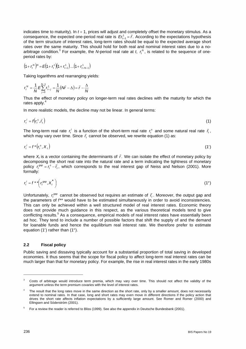
Graph 1

Ex ante real interest rates

0

2

4

6

8

10

1990 1992 1994 1996 1998 2000

Canada

0

2

4

6

8

10

1990 1992 1994 1996 1998 2000

France

0

2

4

6

8

10

1990 1992 1994 1996 1998 2000

Germany

0

2

4

6

8

10

1990 1992 1994 1996 1998 2000

Italy

0

2

4

6

8

10

1990 1992 1994 1996 1998 2000

Japan

0

2

4

6

8

10

1990 1992 1994 1996 1998 2000

Norway

0

2

4

6

8

10

1990 1992 1994 1996 1998 2000

Spain

0

2

4

6

8

10

1990 1992 1994 1996 1998 2000

Sweden

0

2

4

6

8

10

1990 1992 1994 1996 1998 2000

United Kingdom

0

2

4

6

8

10

1990 1992 1994 1996 1998 2000

10 year real rate 5 year real rate

United States


4. Long-term ex ante real interest rates since the 1990s

Graph 1 shows five-year and 10-year ex ante real rates for 10 industrialised countries. The sample period begins in 1989, when Consensus Forecasts for CPI inflation are first available for Canada, France, Germany, Italy, Japan, the United Kingdom and the United States. In 1995, Spain and Sweden are added to the list, and in 1998 Norway. A second data constraint is the availability of nominal interest rates of the desired maturity. This is particularly relevant in the case of Japan, which did not introduce five-year bonds before the late 1990s.

As can be seen from Graph 1, ex ante real interest rates in industrialised countries declined during most of the 1990s and have remained in a relatively narrow corridor ranging from just under 2% to just over 4%. The mean five-year ex ante real rate halved from 6.5% in early 1990 to 3.2% in late 1999, and the development of 10-year real rates has been similar. The decline in real interest rates was briefly interrupted during 1993/94, but they soon reverted to their downward trend, which continued until 1998. They increased somewhat during the following years, but eased again in 2001.

The only, although important, exception to this overall picture is the United States. US real rates were much lower than those in other countries during the first half of the 1990s, although they too were declining. Between 1994 and 1997, however, US rates remained relatively constant between 3 and 4%, and declined only in 1998 in line with those of the other countries of our sample.

The 1990s also saw a remarkable convergence of the real interest rates in all countries bar Japan. The difference between the minimum and the maximum rate at a single point in time declined from 4-5 percentage points in the early 1990s to 1-2 percentage points towards the end of the decade. The main factor behind this convergence was the sharp decline in the real interest rates of Italy, Spain and Sweden. During the early 1990s, Italy had by far the highest rates in our sample.10 In 1992, five-year ex ante real interest rates were 4 percentage points higher than those in France and 5 percentage points higher than the corresponding German rates. In 1999, the difference declined to a few basis points. Ex ante rates for Spain and Sweden are available only as from 1995, so we cannot say much about the first half of the 1990s. But we see real interest rate convergence even during the sample that is available. In early 1995, Spanish real interest rates stood at 7.3%, compared to 3.7% in Germany. Four years later in 1999, Spanish ex ante rates were half a percentage point lower than German rates. What is interesting is that Swedish rates showed a similar decline, although Sweden is not, and at that time was not expected to be, a member of EMU. This suggests that although monetary union may have been a factor in explaining real rate convergence, it was not the only one.

5. Empirical results

5.1 Explanatory variables and estimation methodology

As we have mentioned in Section 2, economic theory provides little guidance as to what a model for real interest rates should look like. Our approach is therefore rather ad hoc. It relates the level of five- and 10-year ex ante real rates (r05cf and r10cf, respectively) to a monetary policy variable, fiscal variables and a set of controls. A complete list of the variables and their sources is given in Table A1 of the Appendix.

Our monetary policy variable is the three-month money market rate, deflated by inflation over the previous 12 months (r3mre). Since inflation is relatively persistent in the short run, r3mre should be a good proxy for the ex ante real rate. Twelve-month inflation is preferable to three-month inflation for several reasons. Firstly, year-on-year inflation is the headline measure of inflation and should therefore correspond more closely to the expectations of agents than price increases over a shorter time span. Secondly, inflation over short periods may be distorted by temporary factors. This is

10 Italian nominal and real rates declined sharply in the aftermath of its ejection from the EMS in September 1992, but shot up

again about a year later.


reflected by the fact that longer-term inflation tends to have better forecasting power for future price developments than short-term price rises. Thirdly, using price increases for periods of under a year forces us to seasonally adjust the data, thus adding to potential mismeasurement.

We measure fiscal policy by gross government debt (ggdgs) and current net borrowing (nbg) or, alternatively, cyclically adjusted net borrowing (nbgca).

Data availability is a big issue when it comes to controlling for shifts in the supply of, or the demand for, funds that are not related to either monetary or fiscal policy.11 Let us begin with the supply of funds, ie saving. Public saving is already captured by our fiscal variable. We proxy private saving by both current and expected GDP growth. According to the permanent income and life cycle hypotheses, household saving should depend on future expected or life income, which we proxy by the Consensus Forecast for GDP growth over the five- and 10-year horizon, respectively (gdp_e5 and gdp_e10). In addition, many studies have found that current income does seem to have an important effect on consumption and saving.12 We therefore include current GDP growth (gdp) as a further explanatory variable for saving.

On the demand side, the main driving force of investment is probably expected profitability. We proxy future profitability by the price/earnings ratio (peratio) of the relevant MSCI country index and a competiveness index based on relative price levels (comix). The latter is closely related to the concept of the real exchange rate.13 Both expected and current GDP are also likely to be important driving forces for investment. We control for the possibility that the economy is below its production frontier by including the output gap (y_gap) and unemployment (unrte).

As mentioned before, our measure for the real interest rate may be polluted by an inflation risk premium. We address this issue by including the 12-month inflation rate (pi) as a proxy for inflation risk. This is based on the assumption that a positive relationship exists between the level of the inflation rate and its (expected) variation. Moreover, including the inflation rate as such allows us to say something about the effect of nominal shocks.

In order to avoid any problems arising from having an unbalanced sample, we first present estimates for the countries for which data are available for the whole sample period. We then corroborate the results using the full (unbalanced) sample of countries. The data for the estimations with a balanced panel are biannual (April and October) and end in the first half of 2002. In the case of the five-year rate, they start in April 1990, in the case of the 10-year rate in the first half of 1991, leaving us with a maximum of 25 periods and 23 periods for a given country, respectively. In the case of the five-year rate, this maximum number of observations is reached by Canada, the United States, the United Kingdom, France, Italy and Germany, in the case of the 10-year rate by the same group of countries and also by Japan.

Unfortunately, the comparatively small cross-sectional dimension of our dataset restricts the range of possible panel estimation methods. This is especially true for dynamic panel estimations like GMM à la Arellano and Bond (1991), which need a certain minimum number of cross-sectional units. Therefore, due to the low degree of freedom we restrict ourselves to estimating a simple fixed-effects model of the following type:

tttiiti dr ε++β+α= ,, X (3)

Here, ri,t is the respective real rate for country i at time t, αi is a country-specific constant (the “fixed effect”), Xi,t is a matrix of explanatory variables that vary across time and country, dt captures the pure time effect and εt is an error term which is assumed to be independent and identically distributed. For the estimation, the individual means are subtracted from equation (3) (within estimator). This fixed-effects regression amounts to testing whether movements in differences of the longer-term real rates

11 For a list of possible factors determining the supply of and demand for funds, see, for example,

Blanchard and Summers (1984) or Chadha and Dimsdale (1999). 12 Current income will play a direct role if consumers are credit constrained or if income shocks are permanent. 13 If uncovered real interest rate parity holds, then the deviation of a country’s real interest rate from world rates should be

equal to the expected change in the real exchange rate over the maturity of the investment. The expected change in the real exchange rate should be related to the current level if one assumes that PPP holds in the long run, ie over five or 10 years, respectively.


across countries can be attributed to movements in differences of the explanatory variables across countries.

We estimate equation (3) in levels. Although the evidence on whether or not real interest rates are stationary is inconclusive, there is little reason to believe that the deviation of national real rates from the world rate has a unit root. Unfortunately, the small number of observations does not allow us to apply standard unit root tests.

One shortcoming of static regressions such as (3) is that it is difficult to rule out reverse causality from ri,t to the variables contained in Xi,t. We address this problem by repeating the estimation using lagged values of r3mre. This reduces the problem of reverse causality but does not eliminate it, since real interest rates, both short-term and long-term, are fairly persistent. Unfortunately, due to the low number of observations we cannot instrument variables.

5.2 Estimation results

The results of our basic estimations with a balanced panel are presented in Table 1. Let us first turn to the estimation for the five-year real rate that includes all the right-hand variables listed above (regression 1). The coefficient of the short-term real rate r3mre is positive and highly significant. Of the fiscal variables, government debt (ggdgs) and cyclically adjusted net borrowing (nbgca) are significant at the 5% level. Substituting the latter by non-adjusted net borrowing (nbg) does not change the results qualitatively. Of the control variables, expected GDP (gdp_e5), the unemployment rate (unrte), the output gap (y_gap), and the rate of inflation (pi) are statistically significant. The positive coefficient on expected GDP growth suggests that economic growth matters primarily through its impact on the demand for funds (investment) rather than the supply (saving). The negative coefficients on unemployment and the output gap indicate that the real interest rate is lower if the economy operates below potential. Finally, the positive relationship between real interest rates and inflation points towards the existence of an inflation risk premium.

In order to obtain a more parsimonious model, we sequentially reject the least significant variable until only significant variables remain. The results are given in the second column of Table 1 (regression 2). Only variables that were significant in the general model remain so in the smaller regression. In the process of reducing the number of coefficients, the output gap also drops out. The other previously significant variables remain significant and keep their signs. Moreover, both the coefficient estimates and their standard errors are of comparable size.

Let us now turn to the results for the 10-year rate given in columns 4 and 5 of Table 1. Note that the sample now also includes Japan, for which five-year rates were not available for the whole estimation period. In order to ensure comparability, we repeat the regression excluding Japan (columns 7-9). We find that the coefficient of the three-month rate (r3mre) is highly significant but slightly smaller relative to what we found in the previous regressions. The results concerning the fiscal variables depend on whether or not the sample includes Japan. If Japan is included (column 4), then the fiscal variables turn out to be insignificant if both net borrowing (nbg or nbgca, respectively) and government debt (ggdgs) are included. However, government debt becomes significant if we drop net borrowing (see regression 5) and vice versa. If we exclude Japan (regression 7), government debt ggdgs is significant at the 5% level. Among the control variables, only the price/earnings ratio (perat) and the rate of inflation (pi) are significant at the 1% level. The remaining variables are always insignificant at the conventional confidence levels.

244 B

IS Papers N

o 19

Table 1

Results from fixed-effects estimation of basic specification

r05cf r10cf (including Japan) r10cf (excluding Japan)

Full sample period Sample split (98:01) Full sample period Sample split (98:01) Full sample period Sample split (98:01)

Explanatory variables

1 2 3 4 5 6 7 8 9

r3mre 0.5171** (0.0438)

0.4883** (0.0422)

0.4652** (0.0445)

−0.0012 (0.1298)

0.4467** (0.0405)

0.3960**(0.0341)

0.4038** (0.0343)

0.0814 (0.0928)

0.4735**(0.0459)

0.4183** (0.0367)

0.4557** (0.0412)

−0.0284 (0.1061)

nbgca 0.0869* (0.0363)

0.0746* (0.0316)

0.0646* (0.0313)

0.0433 (0.0860)

0.0274 (0.0347)

0.0241 (0.0417)

ggdgs 0.0262* (0.0120)

0.0343** (0.0105)

0.0636** (0.0119)

0.0688** (0.0148)

0.0121 (0.0092)

0.0213**(0.0050)

0.0251** (0.0069)

0.0137 (0.0077)

0.0283* (0.0127)

0.0393** (0.0089)

0.0474** (0.0104)

0.0422** (0.0129)

gdp 0.0115 (0.0348)

0.0246 (0.0343)

0.0557 (0.0358)

gdp_e5/10 0.6157** (0.2177)

0.4724* (0.1872)

0.3487 (0.1969)

0.4979 (0.3417)

0.1156 (0.1955)

−0.0731 (0.3047)

unrte −0.1915** (0.0675)

−0.1092* (0.0496)

−0.1857** (0.0549)

−0.3758** (0.1025)

0.0842 (0.0700)

0.1379 (0.0784)

y_gap −0.1377* (0.0659)

−0.0468 (0.0687)

−0.0293 (0.0716)

comix −0.0075 (0.0066)

−0.0086 (0.0062)

0.0003 (0.0072)

perat 0.0163 (0.0191)

0.0362** (0.0108)

0.0320**(0.0097)

0.0332** (0.0102)

−0.0023 (0.0220)

0.0547**(0.0203)

0.0527** (0.0194)

0.0583** (0.0210)

0.0216 (0.0396)

pi 0.3932** (0.0562)

0.3569** (0.0511)

0.3095** (0.0525)

0.1304 (0.1279)

0.4354** (0.0658)

0.3702**(0.0514)

0.3445** (0.0525)

0.2619* (0.1061)

0.4429**(0.0695)

0.3453** (0.0561)

0.3371** (0.0578)

0.2518* (0.1220)

BIS P

apers No 19

245

Table 1 (cont)

Results from fixed-effects estimation of basic specification




1 2 3 4 5 6 7 8 9

Sample period 90:01-02:01 90:01-02:01 90:01-02:01 91:01-02:01 91:01-02:01 91:01-02:01 91:01-02:01 91:01-02:01 91:01-02:01

No of periods 25 25 25 23 23 23 23 23 23

Countries 6: DE, FR, IT, CA, UK,

US

6: DE, FR, IT, CA, UK,

US

6: DE, FR, IT, CA, UK, US 7: DE, FR,IT, CA, UK,

US, JP

7: DE, FR,IT, CA, UK,

US, JP

7: DE, FR, IT, CA, UK, US, JP


US


US

6: DE, FR, IT, CA, UK, US

No of obs 150 150 150 161 161 161 138 138 138

R2(w); R2(b) 0.92; 0.74 0.92; 0.76 0.93; 0.55 0.87; 0.86 0.86; 0.62 0.88; 0.59 0.89; 0.96 0.88; 0.85 0.90; 0.82

F-test (p-val) 0.015 0.001 0.000 0.002 0.000 0.000 0.066 0.000 0.000

Time dummies yes yes yes yes yes yes yes yes yes

Note: Standard deviations in brackets; */** = significant at the 1% and 5% levels.


How stable are these results over time? In particular, did EMU affect the determination of long-term real interest rates? We try to shed more light on these questions by splitting the sample in early 1998.14 Although EMU did not take place until a year later, by that time markets already anticipated with reasonable certainty which countries would participate and which would remain outside. The output of the split-sample regressions for the five-year rate are given in column 3 of Table 1 and those for the 10-year rate in columns 6 and 9. In all three cases, the coefficient of the short-term real rate becomes insignificant in the second subperiod, indicating that the effect of monetary policy on long-term real rates lost strength after the beginning of 1998. The results concerning fiscal policy are less clear. The coefficients on debt are highly significant and positive in both subperiods as long as Japan is excluded from the sample. If we include Japan, it ceases to be significant after 1998.

To sum up, the short-term real rate is significant in all regressions in the first period but not in the second. In contrast to the short-term interest rate, there is no general evidence that fiscal policy has lost its importance in the late 1990s. Only in the case of 10-year real rates for the sample including Japan do we find that government debt is significant before 1998, but not afterwards (Table 1, regression 6). This suggests that the high level of Japanese debt combined with low real interest rates since the late 1990s drove the results for the full sample. Japan should therefore be viewed as an exception. In all other cases, we cannot statistically reject equality of coefficients for the two subsamples.

5.3 Robustness

In order to check the robustness of the results with respect to changes in the specification, we rerun the estimations (a) with an alternative estimation method, (b) with dummy variables that control for EMU countries, (c) with a lagged short-term interest rate and (d) for the whole (ie unbalanced) sample.

(a): given that we cannot assume that there is no cross-country correlation in the included variables and that there is no autocorrelation within the variables of a given country, we reestimate the models with Feasible GLS. This allows for heteroskedastic panels, cross-country correlation and country-specific AR1 coefficients. Given the small size of our sample, however, it is unlikely that FGLS is efficient. The results given in Table A2 in the Appendix should therefore merely be used as a robustness check of the results of the basic fixed-effect regressions. As it turns out, the results obtained over the full sample period, namely that the short-term real interest rate and fiscal policy that significantly determine long-term real rates, are confirmed. But we no longer find that the effect of short-term real rates weakens over time.

(b): an obvious candidate explanation for the structural break found in regressions 3-9 of Table 1 is, of course, EMU, which constrains nominal rates in the member countries to be essentially identical.15 As a consequence, differences in real interest rates are mainly due to different inflation expectations. A country with an overheated economy will therefore have lower real rates than a country where the economy operates below potential - just the opposite of what one would normally expect. In order to test for possible EMU effects, we define a dummy variable which is equal to one for EMU countries (DE, FR, IT) on and after 1998:1, but zero otherwise. We interact this dummy with the monetary and fiscal variables, as well as the controls that showed significant coefficients in the previous regressions, and estimate this augmented model. The results of this exercise are reproduced in Table A3 (see Appendix). The EMU variables turn out to be insignificant in all cases, suggesting that the break we found in Table 1 cannot merely be attributed to EMU but is a more general phenomenon.

(c): we try to reduce the problem of reverse causality between r3mre on the one hand, and r5cf and r10cf on the other, by substituting the current short rate with its value lagged by one period (Table A4 in the Appendix). We generally find that monetary policy and fiscal policy are significant determinants of long-term real rates (regressions 2, 5 and 8), although for some reason cyclically adjusted

14 The results are virtually identical if the split date is 1997:2 or 1998:2. 15 Assuming that premia for default and liquidity risk are of minor importance.


government borrowing seems to perform better that debt. In addition, the result that monetary policy seems to have lost strength is confirmed (regressions 3, 6 and 9), whereas the evidence concerning fiscal policy is more mixed. In the case of the 10-year rate, estimates for the sample excluding Japan show a highly significant coefficient for cyclically adjusted net borrowing in the first subperiod, but an insignificant coefficient for the second subperiod. In the regressions without Japan, government borrowing is either always insignificant (five-year rates) or always significant (10-year rates).16

(d): we repeat the estimates using the unbalanced panel of 10 countries for which at least some observations are available. The results are collected in Table A5 of the Appendix. Apart from some differences concerning the control variables, they largely confirm previous estimates as long as we only look at the entire sample period. If we split the sample in 1998, important differences to previous results appear. In particular, the evidence that monetary policy has lost its impact after 1998 cannot be corrobated. With one exception (regression 9), the coefficient on the short-term real rate remains significant, although the point estimates become somewhat smaller. Fiscal policy appears to be equally effective throughout the 1990s and early 2000s, at least outside Japan.

5.4 Discussion

Our estimates indicate that the short-term real interest rate is one of the main factors driving long-term real interest rates. In all our regressions over the full sample ranging from the early 1990s to spring 2002, lower short-term real rates are ceteris paribus associated with lower long-term real rates. This result is robust to changes in the estimation method or in the composition of the sample. However, we find some evidence that the effect of short-term real rates on long-term rates has on average become less strong in recent years. In most of our regressions, the coefficient for the short-term real interest rate turns out to be insignificant in estimations covering only the later part of our sample. This is not simply the result of EMU but applies also to the countries outside the euro area. In part, this may be due to the fact that both short-term and long-term real interest rates have become more synchronised across countries, leaving less variation for our model to exploit. This is compatible with the hypothesis that the relative importance of world factors, or at least international factors, for national long-term real rates has increased over time. This result is in line with the findings of the empirical literature on real rates, for example Pain and Thomas (1997) and Fountas and Wu (1999, 2000). Since our estimation methodology is based on the differences between countries, it is not surprising that we do not obtain significant coefficient estimates.

If it is true that monetary policy can control short-term real rates, then our results - if taken at face value - suggest that monetary policy provides a powerful tool to influence long-term real interest rates. However, can we safely take them at face value? One reason for scepticism is potential reverse causation from long-term real rates to the stance of monetary policy. For example, if long-term real interest rates are high because the economy is expected to grow rapidly over the next few years, inflationary fears may force the central bank to raise short-term interest rates. Nevertheless, the fact that our results basically hold even if we use lagged short real rates suggests that reverse causation is not the whole story.

Our results concerning fiscal variables are less clear than those for the short-term real rate, although this seems to be driven mainly by the Japanese experience of the late 1990s and afterwards. If one drops Japan, then gross government debt turns out to be an important driving force for real interest rates, suggesting that Ricardian equivalence does not hold. The results concerning cyclically adjusted government borrowing are less robust.

Our results are by and large in line with the existing empirical literature, which has up to now concentrated on time series econometrics and not on panel methods. Blanchard and Summers (1984) find that the high real interest rates of the late 1970s and the early 1980s were probably due to the fiscal-monetary policy mix. Fiscal factors are also stressed by Barro and Sala-i-Martin (1990) and by Ford and Laxton (1999). Breedon et al (1999) also stress the importance of domestic factors in determining long-term real interest rates, among them the government debt-to-GDP ratio and real

16 These results hold if we use government debt instead of net borrowing.


short-term rates. The role of monetary policy is stressed by Allsopp and Glyn (1999), who conclude their paper with the statement that their analysis leads them “... to conclude that it would be wrong to think of the real interest rate as determined ... independent of monetary policy” (p 15).

As in the case of real interest rates, our results concerning fiscal policy represent correlations that do not necessarily indicate causality. Reverse causality may be a problem in particular for net lending. In the long run, high real interest rates add to debt servicing costs and therefore to the government’s financing requirements. Nevertheless, interest payments on the public debt tend to be relatively sticky due to the prevalence of long-term nominal interest rates in most countries of our sample and persistent inflation. This should reduce the problem of reverse causality, especially since we are estimating at a half-yearly frequency.

6. Conclusions

The aim of the paper was to shift the focus of the debate on real interest rates more towards long-term rates. We argue that the analysis of real interest rates is only useful if the time horizon for such rates covers the whole investment period. In the case of capital investment, this can be several years, in the case of saving even decades. Given the importance of long-term real interest rates, it is natural to ask to what extent they can be influenced by macroeconomic policy. In the case of monetary policy, this is the stage where short-term real interest rates become important. In the presence of nominal rigidities, short-term real rates are under the control of monetary policy. Although their direct impact on real variables may be limited, they may have a much greater indirect effect through their influence on long-term rates. This link between monetary policy, proxied by the short-term real interest rate, on the one hand, and long-term real rates on the other, is at the heart of the paper. We also consider the effect of fiscal policy, as proxied by government net borrowing and government debt. In contrast to monetary policy, fiscal policy affects the long end of the term structure directly by changing the demand for loanable funds.

Empirical work on ex ante real interest rates comes with serious measurement problems. One of the reasons why relatively little work has been done in this field is scarcity of data. In the absence of inflation-indexed bonds, real rates cannot be observed directly. We believe that survey evidence on inflation expectations can help us to overcome this problem. These price forecasts can be used to deflate nominal interest rates to yield estimates of ex ante real rates. We discuss the problems associated with survey data in depth, but come to the conclusion that they seem to provide a fairly good approximation to the “true” beliefs of market participants.

Our estimation results suggest that both monetary and fiscal policy generally play an important role in the determination of long-term real interest rates. Nevertheless, the importance of monetary policy for long real rates appears to have diminished since the late 1990s. An obvious candidate explanation for this is EMU, in particular since about half of the countries in our sample belong to the euro area. This is not borne out by the data, however. We find that monetary policy has also lost its impact among the non-EMU countries. This is consistent with evidence that monetary policy has become more synchronised across countries, leaving less room for national real interest rates to diverge. Unfortunately, we cannot say whether this implies that monetary policy has indeed become less effective or whether the countries have simply not tried to steer long-term real interest rates away from the group of countries we consider.

In contrast to monetary policy, there is no evidence outside Japan that a country-specific fiscal policy has become less important over time. Only in Japan have low real interest rates coincided with high debt and government borrowing, thus producing insignificant estimates for the coefficients on the fiscal variables.


Data appendix

Table A1

Variables

Description Source

A. Monetary variables r3mre Three-month real interest rate (nominal rate minus annual inflation

over last 12 months) BIS

B. Fiscal variables

nbg Net borrowing by general government, % of GDP (corresponds to net lending in OECD database, multiplied by −1) OECD

nbgca Net lending by general government, cyclically adjusted, % of GDP OECD

ggdgs General government gross debt, % of GDP OECD

C. Control variables

gdp_e5/10 Real GDP growth expected over the next 5/10 years Consensus Forecast

gdp Growth rate of current GDP, 1995 prices OECD

y_gap Output gap, % of GDP OECD

unrte Unemployment rate OECD

pi Inflation over the previous 12 months OECD

perat Price earnings ratio based on analysts’ forecasts for profits of firms contained in MSCI country index in 12 months’ time I/B/E/S

comix Competitiveness index, based on relative consumer prices OECD

250 B

IS Papers N

o 19

Table A2

Results from FGLS estimation (heteroskedastic panels with cross-country correlation, country-specific AR1)




1 2 3 4 5 6 7 8 9

r3mre 0.4128** (0.0399)

0.4383** (0.0367)

0.4530** (0.0379)

0.3393** (0.0924)

0.3547** (0.0305)

0.3045**(0.0295)

0.3128**(0.0308)

0.2209** (0.0605)

0.3502**(0.0363)

0.2788** (0.0330)

0.3469** (0.0295)

0.0943 (0.0663)

nbgca 0.0530 (0.0310)

0.0010 (0.0221)

0.0146 (0.0316)

ggdgs 0.0360** (0.0110)

0.0370** (0.0098)

0.0352** (0.0101)

0.0349** (0.0112)

0.0035 (0.0076)

0.0056 (0.0047)

0.0078 (0.0048)

0.0012 (0.0058)

0.0285* (0.0121)

0.0322** (0.0121)

0.0370** (0.0096)

0.0345** (0.0108)

gdp −0.0275 (0.0234)

0.0217 (0.0191)

0.0209 (0.0204)

gdp_e5/10 0.5049** (0.1776)

0.5011** (0.1526)

0.5189** (0.1686)

0.3042 (0.3313)

−0.1640 (0.1228)

0.0716 (0.1949)

unrte −0.1144 (0.0648)

0.0795 (0.0496)

0.1444* (0.0581)

y_gap −0.0155 (0.0445)

0.0342 (0.0339)

0.0506 (0.0374)

comix −0.0024 (0.0049)

−0.0072* (0.0036)

−0.0018 (0.0042)

perat −0.0225 (0.0183)

0.0141 (0.0083)

0.0035 (0.0155)

pi 0.2897** (0.0453)

0.3070** (0.0420)

0.3056** (0.0416)

0.2849** (0.0903)

0.3469** (0.0371)

0.2533**(0.0361)

0.2188**(0.0412)

0.1968** (0.0637)

0.3131**(0.0456)

0.2224** (0.0413)

0.2633** (0.0407)

0.1654** (0.0579)

BIS P

apers No 19

251

Table A2 (cont)

Results from FGLS estimation (heteroskedastic panels with cross-country correlation, country-specific AR1)




1 2 3 4 5 6 7 8 9

Sample period 90:01-02:01 90:01-02:01 90:01-02:01 91:01-02:01 91:01-02:01 91:01-02:01 91:01-02:01 91:01-02:01 91:01-02:01

No of periods 25 25 25 23 23 23 23 23 23


US


US


US, JP


US, JP



US


US


No of obs 150 150 150 161 161 161 138 138 138

Cross-country correlation

yes yes yes yes yes yes yes yes yes

Country-specific AR1

yes yes yes yes yes yes yes yes yes




Table A3

Results from fixed-effects estimation: testing for the effects of EMU

r10cf r05cf

Including Japan Excluding Japan Explanatory variables

1 2 3

EMU EMU EMU

r3mre 0.4863** (0.0484)

−0.1828 (0.2176)

0.3836** (0.0409)

−0.0581 (0.1940)

0.4102** (0.0470)

−0.1259 (0.2073)

nbgca 0.0791* (0.0342)

−0.1224 (0.1214)

ggdgs 0.0434** (0.0136)

−0.0043 (0.0120)

0.0160** (0.0056)

−0.0120 (0.0068)

0.0355** (0.0137)

−0.0037 (0.0086)

gdp_e5/10 0.4267* (0.1915)

−0.1288 (0.4990)

unrte −0.0681 (0.0523)

0.0943 (0.1383)

perat 0.0231* (0.0104)

0.0555 (0.0290)

0.0467* (0.0209)

0.0351 (0.0326)

pi 0.35113** (0.0564)

−0.0753 (0.2838)

0.3421** (0.0584)

−0.0045 (0.1973)

0.3372** (0.0649)

−0.1150 (0.2311)

Sample period 90:01-02:01 91:01-02:01 91:01-02:01

No of periods 25 23 23

Countries 6: DE, FR, IT, CA, UK, US 7: DE, FR, IT, CA, UK, US, JP 6: DE, FR, IT, CA, UK, US

No of obs 150 161 138

R2(w); R2(b) 0.92; 0.74 0.87; 0.80 0.88; 0.86

F-test (p-val) 0.004 0.000 0.025

Time dummies yes yes yes


BIS P

apers No 19

253

Table A4

Results from fixed-effects estimation: including lagged short-term interest rate




1 2 3 4 5 6 7 8 9

r3mre (−1) 0.2483**

(0.0544)

0.2199** (0.0476)

0.1820**(0.0525)

−0.1102 (0.1531)

0.2258**(0.0450)

0.2398**(0.0422)

0.2608**(0.0446)

0.1097 (0.1214)

0.2196**(0.0544)

0.2282**(0.0455)

0.2527**(0.0493)

0.0804 (0.1459)

nbgca 0.1726** (0.0520)

0.1958** (0.0358)

0.1494**(0.0406)

0.2446* (0.0989)

0.0466 (0.0446)

0.0644**(0.0231)

0.0368 (0.0321)

−0.0338 (0.0682)

0.0987 (0.0588)

0.1375**(0.0378)

0.1080**(0.0407)

0.0129 (0.0824)

ggdgs 0.0158 (0.0173)

0.0227 (0.0117)

0.0214 (0.0191)

gdp −0.0377 (0.0476)

−0.0153 (0.0438)

0.0052 (0.0475)

gdp_e5/10 0.3028 (0.3008)

0.0726 (0.2515)

−0.2161 (0.4084)

unrte −0.3565** (0.0912)

−0.3574** (0.0568)

−0.4025**(0.0663)

−0.6155**(0.1002)

−0.0653 (0.0881)

−0.0409 (0.0974)

y_gap 0.0034 (0.0889)

0.0562 (0.0873)

0.0661 (0.0943)

comix −0.0051 (0.0092)

−0.0062 (0.0080)

0.0005 (0.0096)

perat −0.0117 (0.0267)

0.0312* (0.0139)

0.0293 (0.0269)

pi 0.1143 (0.0693)

0.2088**(0.0803)

0.2359**(0.0646)

0.2498**(0.0727)

0.0535 (0.1563)

0.1956* (0.0878)

0.2321**(0.0739)

0.2532**(0.0820)

0.0429 (0.1839)

254

BIS P

apers No 19

Table A4 (cont)

Results from fixed-effects estimation: including lagged short-term interest rate




1 2 3 4 5 6 7 8 9

Sample period 90:01-02:01 90:01-02:01 90:01-02:01 91:01-02:01 91:01-02:01 91:01-02:01 91:01-02:01 91:01-02:01 91:01-02:01

No of periods 25 25 25 23 23 23 23 23 23


US

6: DE, FR, IT, CA, UK,

US


US, JP


US, JP



US


US


No of obs 149 149 146 161 161 154 138 138 132

R2(w); R2(b) 0.85; 0.09 0.84; 0.18 0.86; 0.48 0.79; 0.09 0.77; 0.87 0.78; 0.91 0.80; 0.81 0.79; 0.74 0.80; 0.82

F-test (p-val) 0.000 0.000 0.000 0.000 0.000 0.000 0.066 0.020 0.000



BIS P

apers No 19

255

Table A5 Results from fixed-effects estimation: unbalanced sample

r05cf (excluding Japan) r10cf (including Japan) r10cf (excluding Japan)



1 2 3 4 5 6 7 8 9

r3mre 0.5787** (0.0362)

0.5752**(0.0341)

0.5776**(0.0392)

0.4372**(0.0891)

0.4564**(0.0327)

0.4403**(0.0319)

0.4342**(0.0329)

0.2718**(0.0735)

0.4529**(0.0360)

0.4392**(0.0339)

0.4554**(0.0372)

0.1564 (0.0843)

nbgca 0.0479 (0.0320)

0.0123 (0.0303)

0.0099 (0.0352)

ggdgs 0.0245* (0.0107)

0.0379**(0.0081)

0.0391**(0.0089)

0.0369**(0.0107)

0.0135 (0.0081)

0.0059 (0.0045)

0.0084 (0.0058)

−0.0034 (0.0061)

0.0287* (0.0112)

0.0315**(0.0082)

0.0343**(0.0086)

0.0298** (0.0104)

gdp 0.0505** (0.0318)

0.0449 (0.0300)

0.0904**(0.0266)

0.1024**(0.0270)

0.1597* (0.0705)

0.0531 (0.0310)

gdp_e5/10 0.7146** (0.1915)

0.7937**(0.1713)

0.8150**(0.1898)

0.5977* (0.2892)

0.2837 (0.1588)

0.2510 (0.2361)

unrte −0.0791 (0.0498)

0.0939 (0.0477)

0.1081* (0.0497)

y_gap −0.2005** (0.0607)

−0.0865* (0.0381)

−0.1111**(0.0413)

0.0590 (0.0775)

−0.0853 (0.0568)

−0.1755**(0.0432)

−0.2108**(0.0451)

−0.1016 (0.0719)

−0.0696 (0.0619)

−0.0886* (0.0372)

−0.1205**(0.0390)

0.0792 (0.0730)

comix −0.0055 (0.0060)

−0.0094 (0.0055)

−0.0024 (0.0061)

perat 0.0033 (0.0164)

0.0256**(0.0098)

0.0317 (0.0163)

pi 0.4867** (0.0495)

0.4643**(0.0465)

0.4522**(0.0490)

0.3563**(0.1054)

0.4480**(0.0463)

0.4524**(0.0467)

0.4397**(0.0465)

0.3292**(0.0872)

0.4433**(0.0488)

0.3858**(0.0432)

0.3761**(0.0434)

0.1493 (0.0978)

256

BIS P

apers No 19

Table A5 (cont)

Results from fixed-effects estimation: unbalanced sample

r05cf (excluding Japan) r10cf (including Japan) r10cf (excluding Japan)



1 2 3 4 5 6 7 8 9

Sample period 89:02-02:01 89:02-02:01 89:02-02:01 89:02-02:01 89:02-02:01 89:02-02:01 89:02-02:01 89:02-02:01 89:02-02:01

Max no of periods 26 26 26 26 26 26 26 26 26

Countries 9: DE, FR, IT, CA, UK, US, ES, NO,

SE

9: DE, FR, IT, CA, UK, US, ES, NO,

SE

9: DE, FR, IT, CA, UK, US, ES, NO, SE

10: DE, FR,IT, CA, UK, US, JP, ES,

NO, SE

10: DE, FR,IT CA, UK, US, JP, ES,

NO, SE

10: DE, FR, IT, CA, UK, US, JP, ES, NO, SE

9: DE, FR IT, CA, UK, US, ES, NO,

SE

9: DE, FR,IT, CA, UK, US, ES, NO,

SE

9: DE, FR, IT, CA, UK, US, ES, NO, SE

No of obs 192 192 192 214 214 214 188 188 188

R2(w); R2(b) 0.91; 0.78 0.91; 0.67 0.91; 0.67 0.90; 0.70 0.89; 0.85 0.90; 0.84 0.91; 0.71 0.90; 0.76 0.91; 0.71

F-test (p-val) 0.019 0.000 0.000 0.000 0.000 0.000 0.002 0.000 0.000




References

Al Awad, M and B K Goodwin (1998): “Dynamic linkages among real interest rates in international capital markets”, Journal of Money and Finance, vol 17, pp 881-907. Allsop, C and A Glyn (1999): “The assessment: real interest rates”, Oxford Review of Economic Policy, vol 15, no 2, pp 1-16. Arellano, M and S R Bond (1991): “Some tests of specification for panel data: Monte Carlo evidence and an application to employment equations”, Review of Economic Studies, vol 58, pp 277-97. Barro, R J and X Sala-i-Martin (1990): “World real interest rates”, NBER Working Paper, no 3317, April. Blanchard, O J and L H Summers (1984): “Perspectives on high world real interest rates”, Brookings Papers on Economic Activity, vol 2, pp 271-324. Bliss, C (1999): “The real rate of interest: a theoretical analysis”, Oxford Review of Economic Policy, vol 15, no 2, pp 46-58. Breedon, F, B Henry and G Williams (1999): “Long-term real interest rates: evidence on the global capital market”, Oxford Review of Economic Policy, vol 15, no 2, pp 128-42. Buraschi, A and A Jiltsov (2002): Is inflation risk priced?, London Business School, mimeo. Chadha, J S and N H Dimsdale (1999): “A long view of real rates”, Oxford Review of Economic Policy, vol 15, no 2, pp 17-45. Deacon, M and A Derry (1998): Inflation-indexed securities, Prentice Hall Europe, London. Deutsche Bundesbank (2001): “Real interest rates: movements and determinants”, Monthly Report, July, pp 31-47. Ellingsen, T and U Söderström (2001): “Monetary policy and market interest rates”, American Economic Review, vol 91, no 5, pp 1594-607. Fisher, I (1930): The theory of interest, New York. Ford, R and D Laxton (1999): “World public debt and real interest rates”, Oxford Review of Economic Policy, vol 15, no 2, pp 77-94. Fountas, S and J-L Wu (1999): “Testing for real interest rate convergence in European countries”, Scottish Journal of Political Economy, vol 46, no 2, May, pp 158-74. ——— (2000): “Real interest rate parity under regime shifts and implications for monetary policy”, The Manchester School, vol 68, no 6, December, pp 685-700. Keynes, J M (1936): The General Theory of Employment, Interest and Money, London.

Kraemer, J W (1996): “Determinants of the expected real long-term interest rates in the G7 countries”, The Kiel Institute of World Economic Working Paper, no 751, June. Laster, D, P Bennett and I S Geoum (1999): “Rational bias in macroeconomic forecasts”, Quarterly Journal of Economics, vol 114, no 1, 293-318. Neiss, K S and E Nelson (2001): “The real interest rate gap as an inflation indicator”, Bank of England Working Paper, no 130. Orr, A, M Edey and M Kennedy (1995): “The determinants of real long-term interest rates: 17 country pooled-time-series evidence”, OECD Economics Department Working Papers, no 155. Pain, D and R Thomas (1997): “Real interest rate linkages: testing for common trends and cycles”, Bank of England Working Paper, no 65. Romer, C D and D H Romer (2000): “Federal Reserve information and the behavior of interest rates”, American Economic Review, vol 90, no 3, pp 429-57. Scott, M (1993): “Real interest rates: past and future”, National Institute Economic Review, no 143, pp 54-71. Wicksell, K (1898): Geldzins und Güterpreise, Jena. Woodford, M (2002): “A neo-Wicksellian framework for the analysis of monetary policy”, Chapter 4 in Interest and Prices, unpublished manuscript. Wu, J-L (1999): “A re-examination of the exchange rate-interest differential relationship: evidence from Germany and Japan”, Journal of International Money and Finance, vol 18, pp 319-36.

Real long-term interest rates and monetary policy: a cross ... · Real long-term interest rates and...

Documents

Transcript of Real long-term interest rates and monetary policy: a cross ... · Real long-term interest rates and...