Real financial models in Argentina

Dario Debowicz

Job Market Paper

Abstract

The significant real effects arising from the present worldwide financial crisis suggest

that the workings of the financial sphere significantly affect the value of social

production, the distribution of income and wealth, and the magnitude of income

poverty, all important social welfare indicators. Reflecting this, in the present paper a

set of nested models is built, departing from a real-focused single-country CGE model

targeted to a developing economy (the IFPRI Standard Model). The model extensions

account for the workings of the financial sphere and „money in the production function‟,

the latter in the tradition started by Milton Friedman (1969). The models are then

applied in a stylized way to identify the short and medium run effects of an increase in

the perceived probability of default on domestic assets in Argentina, finding significant

short-run effects on the activity level and distribution. For validation purposes, a set of

elasticity values coming out of the model is compared against econometric estimates.

1

Table of Contents

1. Introduction ............................................................................................................... 3 2. Models ....................................................................................................................... 4

3. Calibration ............................................................................................................... 13 4. Simulations .............................................................................................................. 14 5. Sensitivity analysis and model validation ............................................................... 25 6. Conclusions ............................................................................................................. 26 Annex I. Brief review of financial CGE models ............................................................. 30

Annex II. Mathematical statement of the model ............................................................. 32

Annex III. Derivation of demanded asset shares ............................................................ 56 Annex IV. Results of additional external shocks ............................................................ 58

Annex V. Results of sensitivity analysis ......................................................................... 59 Annex VI. Bibliography .................................................................................................. 62

2

1. Introduction

The international debate on the effects of the last wave of globalization on the levels of

activity, employment and income distribution in developing countries allow us to

identify the channels at stake. Besides, given that the channels and effects depend on

important and interesting ways on developing-economy specific characteristics (Agenor

and Montiel 1999) and on country-specific characteristics (Goldberg and Pavcnik 2007,

p.41), a model suitable to evaluate these channels in a quantitative way should account

for the structural characteristics common to developing countries and be easily

adaptable to country-specific features.

As pointed out by Pierre-Richard Agenor and Peter Montiel (1999, p.4), development

macroeconomic commonalities that the model should account for include the usefulness

of a three good (exportables, importables and non-tradables) disaggregation of

production, informal markets, public sector production, imported intermediate goods,

labor market segmentation and working capital, characteristics which are also present in

developed economies but are more crucial in developing ones.

Also, acknowledging that the evolution of the specific forms of savings and asset stocks

is an essential part of the economic process (Tobin 1981,p.13) and the relevance of the

real-financial links (clearly illustrated by the series of financial crisis hitting LDCs and

the recent crisis originated in developed countries with worldwide reverberation), the

model should include the workings of the financial sphere and the critical transmission

channels linking it to the real side.

Lastly, to provide analysts with a wide spectrum of policy options, the model should

include a rich variety of macroeconomic policy instruments, including different tax

rates, government expenditures (disentangling transfers, public consumption and public

investment), deficit monetization, rediscount levels, rediscount rates, and bank required

reserve ratios.

The overall goal of this paper is to build such a model, placing it in the perspective of

existing models and analyzing its workings. Section 2 presents the modeling strategy,

describing a set of nested models built in the context of existing financial computerized

3

general equilibrium (CGE) models. Section 3 goes through the models calibration.

Section 4 analyzes the models workings, hitting them with an external shock. Section 5

deals with sensitivity analysis and models validation against econometric estimates.

Section 6 concludes.

2. Models

The macroeconomic financial CGE modeling framework seems to be the best one for

the case at stake, since it allows to: i) model explicitly the markets of goods, factors and

assets (Bourguignon and Pereira da Silva 2003, pages 12-18); ii) capture the inter-

linkages between macro-level changes in the stocks of financial assets and levels of

activity and employment (prone for macro analysis) and a structural adjustment story

(prone for CGE analysis); iii) contribute to closing the existing gap between macro and

CGE models (Robinson 2006).

CGE models are essentially structural, capturing market mechanisms explicitly,

specifying demand and supply behaviors with roles for prices and demand and supply

elasticities. Their spirit is essentially microeconomic (Dervis, de Melo et al. 1982, p. 6).

However, in order to gain realism, the factor and products equilibrium concepts that

come from the Arrow-Debreu general equilibrium theory are usually enriched by

additional equilibria concepts and ad-hoc elements. The former include, among others,

flow equilibrium in the market for loanable funds and equilibrium in specific asset

markets. The latter include i) limited substitution elasticities in a variety of important

relationships, ii) absence or lack of proper work of various markets – e.g. restrictions to

factor mobility and price rigidities, and iii) equilibrating mechanisms among macro

aggregate nominal flows - typical in Lance Taylor‟s work - (Robinson 1989).

While traditional CGEs have a single account capturing the “loanable funds” market

work of collecting savings and purchasing capital goods, financial CGE models

elaborate this account (Robinson 1991), adding a set of imperfectly substitutable assets

to capture imperfections in the capital markets. These models are generally designed to

analyze the short and medium run impact on economic performance and income

distribution in developing economies of structural adjustment and stabilization

programs implemented in response to external macro shocks (e.g. increased oil prices,

reduced availability of foreign borrowing). Given their concern with the short and

4

medium run effects on the economy, they tend to directly incorporate macro phenomena

and to have a simple treatment of expectations1. They all break the neoclassical

separation between the real and financial spheres of the economy via using at least one

ad-hoc feature.

A review of financial CGE models2 (tabled in Annex I) evidences that they typically

deal with a large set of financial assets and track the sizes and compositions of the

economic actors‟ portfolios, tracking their holdings of currency, deposits, loans,

required reserves, domestic and foreign bonds, and international reserves, even

differentiating assets by currency of denomination. They capture the link going from the

financial side to the real side in a variety of ways, with the workings of the financial

side hitting the demand and/or the supply for goods. Concerning the former, they reflect

i) the positive effect of real balances on consumption (Easterly 1990); ii) the negative

effect of the real interest rate on physical investment (Bourguignon, Branson et al. 1992;

Thissen 2000); iii) the positive effect of international capital inflows on investment (via

relaxing binding financial constrains, as in Vos(1997)). Concerning the latter, they tend

to reflect it via a “working capital” channel that incorporates firms credit dependency

and was pioneered by Kapur (1976) and Mathieson (1980) (Decaluwe and

Nsengiyumva 1994,p263-4).

The working capital channel has been modeled in three ways: i) letting the cost of

working capital hit the effective production cost of firms and, in turn, the firm‟s desired

level of production, as in the maquette (Bourguignon, Branson et al. 1992) and

IMMPA3 (Agénor, Izquierdo et al. 2003); ii) allowing firms to pass along the cost of

working capital to consumers, as in Taylor (1981); iii) making working capital act as a

constraint to hire real production factors, as in Decaluwe and Nsengiyumva (1994) and

Naastepad (2002). None of these models capture the working capital channel along the

„money in the production function‟ tradition started by Friedman (1969), where the

1 “Long-run models which assume full employment and embody steady-state equilibria with rational (or

model-consistent) expectations will miss most of the action”. (Robinson, 1991) 2 DSGE models were not reviewed given their lack of focus on the structural characteristics of LDCs and

income distribution. McKibbin and Sachs (1989) Global and McKibbin and Wilcoxen (1999) G-Cubed

dynamic GE models of the world economy do have real-financial linkages, but are not concerned with

income distribution or the imperfections in the capital markets.

3 IMMPA stands for Integrated Macroeconomic Model for Poverty Analysis.

5

availability of working capital affects the efficiency with which real factors are used.

The present work seeks to fill this gap.

The modeling strategy followed in this work has a dual purpose:

1. Try and help understand the structural adjustment effects of external shocks, with

emphasis on growth and income inequality in a middle-income country.

2. Contribute to the existing debate over the economic significance of including the

financial sphere in CGE models that David Adam and Adam Bevan (1998) mention.

To facilitate the second of these purposes, rather than building a single FCGE model the

strategy followed here consists of building a set of models increasingly accounting for

the significance of the financial sphere. As shown in the below diagram, the models are

called real model (R), real financial model (RF) and real financial augmented model

(RFA), and are nested in the sense that the latter ones include the former ones but

endogeneizing some variables and including additional equations. The real model is a

non-financial extension of the IFPRI Standard model which, in turn, has a neoclassical

core and captures the structural adjustment effects of liberalization in a conventional

way. The real financial model incorporates the workings of the financial sphere. Lastly,

the augmented model includes endogenous money in the production function. The

models are described below, presenting the equations in Annex II.

Diagram 1. Nested Models

+ Money in the Production Function => RFA MODEL

+ Financial Sphere => RF MODEL

IFPRI-Based Dynamic Real Model

+ Real Extensions => R MODEL

6

Real Model

The Real Model is built as an extension of a well-known non-financial model with a

publicly available code: the IFPRI Standard Model (Lofgren, Lee Harris et al. 2002)

The departures from that model are the following ones:

The complementary relationship between skilled labor and physical capital

evidenced during the last globalization wave is captured via a low elasticity of

substitution among them.

The labor market is segmented into a formal and an informal component, with

imperfect mobility across segments along the lines of Harris and Todaro (1970).

While in the informal segment wages adjust for market-clearing, in the formal one

there is incomplete wage adjustment, with a real wage curve (Blanchflower and

Oswald 1994) reflecting that workers gain negotiating power over their wages as

unemployment falls (Blanchard 2009).

Enterprises retain a fraction of their profits and distribute the rest in the form of

dividends to domestic and foreign equity holders.

Banks and the Central Bank are present in the model. Interest flows are determined

as a relevant interest rate times a relevant stock, but both are fixed, so that the

interest flows simply work as a standard set of fixed transfers.

Savings are investment driven with investment, in turn, being determined by a Q-

type function dependent on the return of physical capital and the financial cost of

acquiring it. Public savings are flexible and depend on a set of fixed tax rates and

endogenous tax bases. Foreign savings include not only net imports and transfers

but also dividends and net interest payments to non-residents. As in the Johansen

version of IFPRI model, household savings vary to assure savings-investment

consistency.

The nominal exchange rate is fixed, capturing the presence of Currency Boards or

administered exchange rate regimes typical of developing countries (Agenor and

Montiel 1999). Foreign savings are determined as a function of the capital inflow

received by the country. The flexibility of the real exchange rate is provided by

changes in the prices of domestic goods, in turn imperfect substitutes from goods

produced in other regions for which the export and import prices are fixed (small

country assumption). The numeraire of the model is the nominal exchange rate.

7

Regions trading with the country are disentangled (e.g. Mercosur vs. rest) allowing

to capture regional-specific changes in trade taxes and trade prices.

The capital account of the balance of payments is captured as the sum of an

exogenous component4 (the sum of variations of non-residents asset holdings) and

an endogenous one (the sum of variations of residents asset holdings).

Real Financial Model

In essence, the extension consists in specifying the workings of a set of financial asset

markets. A natural starting point for this is the specification of the set of assets held by

the different actors, which can be captured in a matrix of assets and liabilities as in

Tobin (1969), with financial stocks in the cells inside the matrix, asset holders in the

column headings and liability holders in the row headings. The financial net wealth of

each actor is given by the sum of the values in its column minus the sum of the values in

its row. The sum of the financial wealth of all the actors is necessarily zero. There are

separate equations to update the financial net wealth5 of households (eq. 104), firms (eq.

105) and the public sector (eq. 82 and 106), and portfolio balance equations for

households (eq. 69), firms (eq. 79), banks (eq. 83) and the Central Bank (eq. 91).

Diagram 2. Matrix of Assets and Liabilities

4 The idea of exogenous international capital was at the heart of the ISS money and finance project, which

sought to correct the imbalance where many macro models saw the capital account as a balancing item

which adjusted to the current account. This view was also applied to aid by Howard White in the early

90s, with the main idea that aid creates deficits rather than fills them (Vos, 1997; White, 1998). 5 Capital gains are not systematically included to avoid over-complicating the model.

House-

holds

Enter-

prises

Govern-

ment

Rest

Of

World

BanksCentral

Bank

Households Loan

Enterprises Equity Equity Loan

Government Bond Bond Bond Bond

Rest of the

World

Deposits

Abroad

Deposit

Abroad

Intern.

Reserves

Commercial

BanksDeposit Deposit Deposits Rediscount

Central

BankCurrency

Required

Reserves

8

The assets returns are then determined in the following way:

The interest rate on deposits in domestic banks is determined using an LM equation

that captures transactions demand and liquidity preference and where, ceteris

paribus, increases in the real stock of money (taken the monetary base divided by

the GDP deflator as a proxy) decrease the interest rate, and increases in transactions

(taking real GDP as a proxy) increase it (eq. 114).

The interest rate on bank loans is determined by the interest rate on deposits

adjusted by the reserves ratio (exogenously determined by the Central Bank) and an

exogenous mark-up rate (eq. 92).

The return on bonds adjusts to clear the bonds market (eqs 93-94).

Sector-specific returns on equity are determined simply by the ratio between after-

tax profits and equity (eq. 95).

Interest rates on Central Bank rediscounts and on bank required reserves in the

Central Bank are exogenously determined by the Central Bank, while return on

deposits abroad is exogenously determined in the international financial markets

(small country assumption).

The assets demands are determined in the following way:

Households assets demand

Capitalist households are assumed to face nor informational difficulties neither

transaction costs to enter into financial markets (as in IMMPA), holding then not only

currency and local-currency-denominated deposits in domestic banks (as skilled and

unskilled households do) but also equity in private firms, bonds, and dollar denominated

deposits in domestic banks and abroad (eq. 69). Reflecting a demand for transaction

motive, currency held by households is proportional to their initial consumption values6.

Skilled- and unskilled households‟ deposits are determined as a residual from their

portfolio balance equation (eq. 69). The allocation of capitalist household deposits into

local- and dollar-denominated deposits follows a fixed rule (eq. 71). The portfolio

allocation of capitalist households among bonds, equity and deposits abroad is

determined maximizing a CES utility function on expected earnings of the assets, as in

Adam and Bevan (1998) (eqs. 72-78). This reflects the perception that agents look at

6 It is kept fixed at the original level, as endogeneizing the households currency holdings proved to break

a critical transmission channel in the augmented model: that going from international capital inflows to

increases in working capital loans.

9

relative returns when deciding portfolio asset shares and have risk aversion (they tend to

avoid corner solutions) in a way which is simple and is not highly data demanding. An

exogenous perceived probability of default on domestic assets is incorporated affecting

their expected return. As in IMMPA, it is implicitly assumed that the potential default

only concerns the interest payments and not capital amortization.

Enterprises assets demand

Firms allocate their financial assets in domestic bank deposits, with its magnitude

determined as the sum of their net financial wealth and borrowed loans (eq. 79). This

means that firms in a given sector simultaneously have deposits and loans, which may

occur due to: a) different contract periods of loans and deposits and b) some enterprises

getting loans while others in the same sector deposit funds into banks.

Rest of the world assets demand

Non-residents hold deposits in domestic banks, equity and bonds, with exogenous flows

altering the values of their stock holdings via updating conditions on its stock holdings.

Commercial banks assets demand

Commercial banks hold required reserves, lend to households and firms, hold public

bonds and deposit abroad. Given that banks profits are transferred at the end of each

period to private sector enterprises, banks net financial wealth remains constant, and

total bank assets are strictly increasing on their liabilities (deposits). Required reserves

are determined by the required reserves ratio times total deposits (eq. 84). The rest of

the portfolio is allocated using a CES utility function (eqs. 85-90), as explained for

capitalist households.

Central Bank assets demand

The Central Bank provides some limited exogenous credit to banks (i.e. rediscounts)

and the public sector (i.e. deficit monetization). The variation of international reserves

held by the Central Bank is the overall result of the balance of payments, which in turn

is assumed to be a constant fraction of the capital account balance (eq. 102) given by

historical data.

Stock flow consistency

Updating conditions are used to accumulate financial flows into financial stocks in the

same period than the flows occur (eqs. 104-112). For example, the stock of foreign

10

deposits in domestic banks in a given period equals the previous one adjusted by the

flow during the given period.

Real Financial Augmented Model

The main transmission channel from the financial to the real sphere is captured along

the „money in the production function‟ tradition started by Friedman (1969).

Specifically, working capital loans are included as a substitutable factor in the CES

production function, affecting the efficiency with which real factors in the formal

segment of the economy are used and, as a result, the overall supply of output and the

structure of production7.

Diagram 3. Money in the production function

As argued by Milton Friedman (1969), the money supply is not necessarily neutral in

the short run: “the separation of the act of sale from the act of purchase (provides money

with a) fundamental productive function” (p.3), such that “(…) real cash balances are at

least in part a factor of production” (p.14).8 This differs from the treatment of working

7 The idea of including working capital in the form of “money in the production function” was suggested

by Sherman Robinson. 8 Friedman illustrates this in the following way: a retailer can economize on his average cash balances by

hiring an errand boy to go to the bank on the corner to get change for large bills tendered by customers.

When it costs ten cents per dollar per year to hold an extra dollar of cash, there will be a greater incentive

to hire the errand boy, that is, to substitute other productive resources for cash. This will mean both a

reduction in the real flow of services from the given productive resources and a change in the structure of

production, since different productive activities may differ in cash-intensity, just as they differ in labor- or

land- intensity” (p.14) (the underline is mine).

Gross Value Added

Value Added Intermediate Aggregate

DomesticAggregateI

InformalUnskilled

AggregateII

Formal Skilled

Physical Capital

Working Capital

Formal Unskilled

Working Capital

Imported

Leontief

CES

CES CES

CES

11

capital in existent FCGE models where either: 1) working capital is totally absent (e.g.

Thissen 2000); 2) working capital is not included in the production function but affects

the effective cost of the real factors (e.g. IMMPA model); 3) working capital acts as a

constraint to hire real production factors (e.g. Decaluwe et al 1994, Naastepad 2002).

A market for working capital is specified, where firms demand and banks supply jointly

determine its level of use and wage. In turn, firms demand is derived from its short-run

profit maximization, together and analogously to their demand for real factors. Banks

supply of working capital is determined as their total asset value times the working

capital asset share coming from the banks‟ maximization of a CES utility function on

asset earnings (eq. 117). The real return on working capital loans adjusts until the

market clears, unless a minimum is hit before, putting a break to the productive use of

working capital and its effect on the activity level (eqs. 116 and 119-120). Together

with inflation, it determines the nominal interest rate on loans9.

By including this transmission channel and linking financial conditions in the country to

external capital flows, the model allows to reflect the influence that external capital

flows have on the activity level, where other FCGE models either neglect the working

capital link (e.g. Thissen 2000) or assume that the domestic country (via the banking

sector) can borrow on world capital markets any amount at the prevailing interest rate

(IMMPA model)10

.

Real Financial Augmented Model – Short Run Closure

In this version, which slightly departs from the RFA model, a minimum real wage for

physical capital is assumed, with capacity utilization becoming flexible when this

minimum is achieved; the wage curve concerns nominal instead of real wages; and the

elasticity in the wage curves are reduced from 0.1 to 0.01 such that the model

approaches the case of nominal wage rigidity. Overall, this version seeks to allow for

higher effects of the shocks considered on aggregate supply.

9 Replacing the LM equation of the Real Financial Model

10 IMMPA assumes that the world supply of loans is perfectly elastic.

12

Disaggregation of actors

The disaggregation of actors in the economy is fairly low to facilitate focusing on the

models workings, but can be easily increased. There are five sectors of activity

(primary, industrial, construction, private services and public services). Factors are

classified in capital and labor, with labor sub-classified in skilled/unskilled and

formal/informal. Finally, there are three representative household groups: skilled wage

recipients, unskilled wage recipients, and capitalist households.

3. Calibration

The parameters of the specified models are calibrated targeting the period of the

Convertibility Plan (1991-2001) in Argentina. Calibration can be conceptualized as

estimation in the special case of under-identification, where the number of parameters to

be estimated exceeds the number of observations. Calibration has become a mainstream

form of empirical investigation in macroeconomics in recent years, providing a

quantitatively informed insight for policy input and facilitating the understanding of the

economic processes at stake, allowing to answering questions of the following type:

Which effects are large? Which are the major stresses under which the economy is

subjected? Are these opposite to received wisdom? If so, why? (Dawkins, Srinivasan et

al. 2001).

The elasticities in the model are choice parameters, except for those in the wage curve

equations (0.10), which are taken from an econometric estimation for Argentina during

the period of the Convertibility Plan done by Damill, Frenkel et al (2002). The value

assigned to elasticity parameters in the production function is 0.8, except for that inside

the skilled-capital composite (0.2), reflecting evidence of low substitution between

skilled labor and physical capital for middle-income countries reported by Agénor et al

(2005,p11). For those in the import-domestic Armington function and export-domestic

CET function, a value of 4.5 is assigned, and for those for import origins and export

destinations 1.5, reflecting especially low substitution and transformation possibilities

between Mercosur area and the rest of the world11

. The elasticity parameters in the LES

consumption function after adjusting for Engel law satisfaction are around 1.10 for the

11 The elasticity parameters in the CES and CET functions (ε) inform the ρ parameters which enter

explicitly in the model, with ρ=1/ε-1 in the CES and ρ=1/ ε +1 in the CET functions.

13

industrial commodity and 0.91 for the others. The semi-elasticity in the investment

function equals 0.2. The migration elasticity among segments of the labor market equals

0.10. Elasticity values of money demand are assumed to be 2.0 respect to interest rate

on deposits and 1.0 respect to real GDP changes. Elasticity values in the CES utility

functions on asset earnings equal 1.05, such that the asset shares in the portfolios of

capitalist households and banks tend to be pretty stable (they would be stable with a

value approaching 1). The annual depreciation of the capital stock was set at 2 %, and

the nominal exchange rate at 1. The sensibility of the balance of payment result to the

capital account balance was calculated as the benchmark ratio of the balance of payment

result and the capital account balance, resulting into 0.203. The natural unemployment

rates are assumed to be rather low (3%). Following the tradition started by Shoven and

Whalley (1972), the remaining parameters are calibrated assuming that the starting

observed point is a solution point of the model. For this purpose, a real-financial SAM

is designed and the values of its cells are assigned at the beginning of the Convertibility

Plan in Argentina (1991).

4. Simulations

The available set of parameters accounting for external shocks – tabulated below-

include five where the impulse to the economy is given essentially via the capital

account of the balance of payments (pdef , RW, ∆𝐷𝐸𝑃 R, ∆𝐸𝑄𝐸

e and ∆𝐵 R) and five via

the trade balance (tmrc,r , terc,r , pwmrc,r , pwerc,r and exr

12). Three of these shocks (tmrc,r ,

terc,r and exr) directly reflect changes in policy instruments.

12

The devaluation simulation also gives an impulse in the investment income component of the current

account and in the capital account, as it changes the dollar-denominated value of assets denominated in

local currency.

14

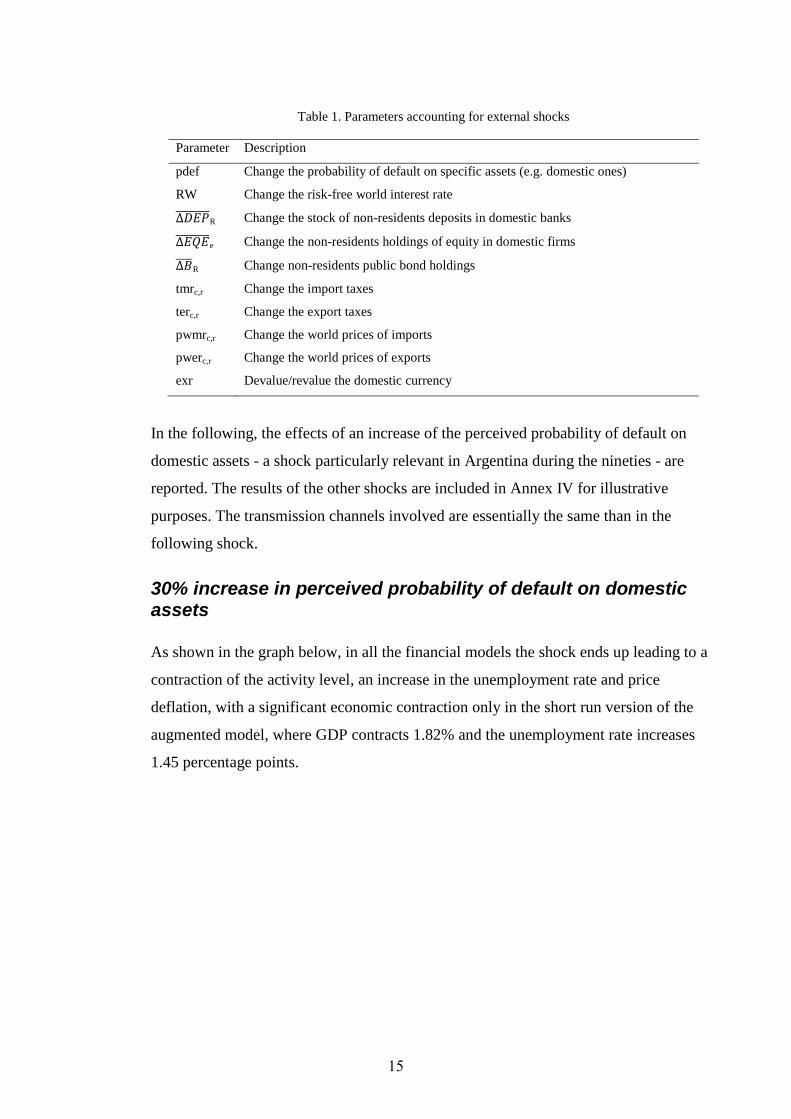
Table 1. Parameters accounting for external shocks

Parameter Description

pdef Change the probability of default on specific assets (e.g. domestic ones)

RW Change the risk-free world interest rate

∆𝐷𝐸𝑃 R Change the stock of non-residents deposits in domestic banks

∆𝐸𝑄𝐸 e Change the non-residents holdings of equity in domestic firms

∆𝐵 R Change non-residents public bond holdings

tmrc,r Change the import taxes

terc,r Change the export taxes

pwmrc,r Change the world prices of imports

pwerc,r Change the world prices of exports

exr Devalue/revalue the domestic currency

In the following, the effects of an increase of the perceived probability of default on

domestic assets - a shock particularly relevant in Argentina during the nineties - are

reported. The results of the other shocks are included in Annex IV for illustrative

purposes. The transmission channels involved are essentially the same than in the

following shock.

30% increase in perceived probability of default on domestic assets

As shown in the graph below, in all the financial models the shock ends up leading to a

contraction of the activity level, an increase in the unemployment rate and price

deflation, with a significant economic contraction only in the short run version of the

augmented model, where GDP contracts 1.82% and the unemployment rate increases

1.45 percentage points.

15

Graph 1. Effects of 30% Perceived Increase in Domestic Assets Default Probability13

Real Model

This model is essentially non financial and as such does not account for the effect of

changes in the perceived probability of default on domestic assets.

Real Financial Model

The shock reduces the expected return on domestic assets, increasing the relative return

of foreign assets and hence giving a signal for the capitalist households to reallocate

their asset portfolio substituting away from domestic into foreign assets. This reduces

the starting net capital inflow, slowing down the accumulation of international reserves

of the Central Bank and cutting the current account deficit that the economy is able to

finance. The withdrawal of deposits from domestic banks reduces the banks‟ asset

portfolio size, leading banks to cut their deposits abroad together with other asset

holdings.

13

Real GDP and domestic price level variations in percentages, unemployment rate variation in

percentage points.

-2.00

-1.50

-1.00

-0.50

0.00

0.50

1.00

1.50

2.00

Real Financial Model

Real Financial Augmented

Model

Real Financial Augmented Short

Run Model

Real GDP

Unemployment rate

Domestic price level

16

Table 2. Balance of Payments

With the nominal exchange rate being fixed, the reduction in the current account deficit

is achieved through domestic deflation that depreciates the real exchange rate and leads

to increase the country‟s trade superavit: the exports value increases and the imports

value falls14

, increasing the share of exports and decreasing that of imports in aggregate

demand.

Table 3. Aggregate Demand Component Shares

Base (%) p.p.15

change

Absorption 98.20 -0.61

Private Consumption 77.35 -0.58

Fixed Investment 15.37 -0.03

Public Consumption 5.49 0.00

Exports 11.22 0.38

Imports -9.43 -0.23

GDP (C+I+G+E-M) 100.00 0.00

With export prices being fixed, producer prices fall proportionately less in the tradable

sectors, providing incentives for the economy to mobilize resources out of construction

and private services sectors towards the sectors producing tradable commodities,

increasing the shares of the primary sector and industry into total value added in order

to increase exports and substitute for imports.

14

Not tabulated. 15

“P.p.” stands for percentage points.

Base (B$) % change

Current Account -8.46 12.16

Trade Balance 3.44 32.72

Exports of Goods and NFS 21.51 2.59

Imports of Goods and NFS 18.07 -3.14

Investment Income -11.90 -0.82

Interests -10.91 -0.97

Profits and Dividends -0.99 0.77

Capital Account 10.62 -12.16

Non Financial Private Sector 7.50 -17.28

Public Sector 1.99 FIXED

Commercial Banks 1.13 0.52

Balance of Payment Result 2.16 -12.16

17

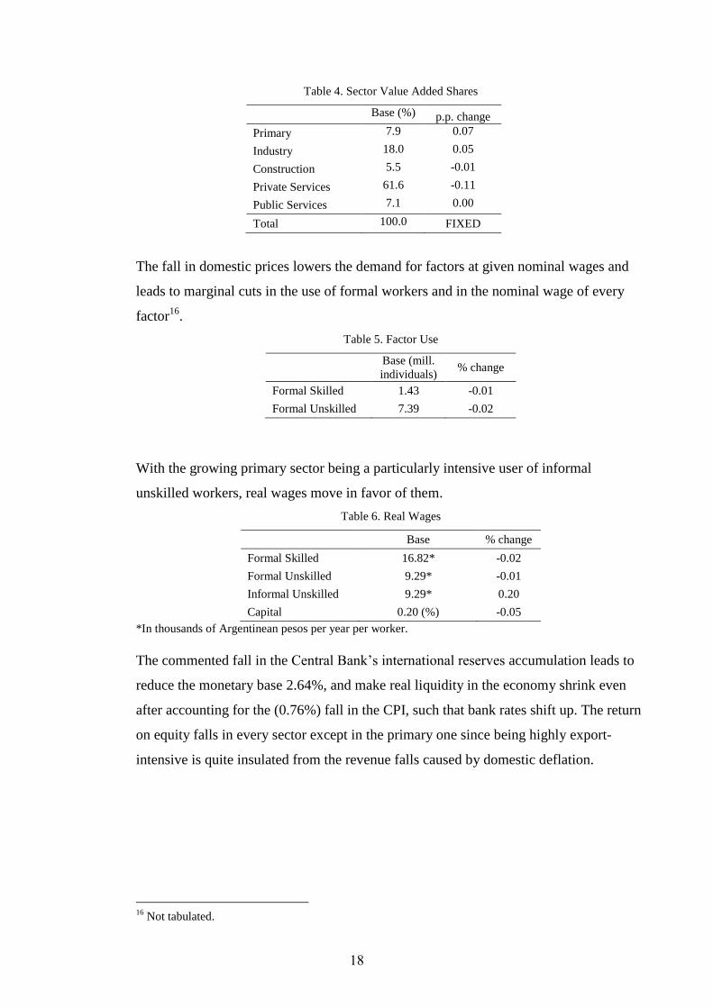
Table 4. Sector Value Added Shares

Base (%) p.p. change

Primary 7.9 0.07

Industry 18.0 0.05

Construction 5.5 -0.01

Private Services 61.6 -0.11

Public Services 7.1 0.00

Total 100.0 FIXED

The fall in domestic prices lowers the demand for factors at given nominal wages and

leads to marginal cuts in the use of formal workers and in the nominal wage of every

factor16

.

Table 5. Factor Use

Base (mill.

individuals) % change

Formal Skilled 1.43 -0.01

Formal Unskilled 7.39 -0.02

With the growing primary sector being a particularly intensive user of informal

unskilled workers, real wages move in favor of them.

Table 6. Real Wages

Base % change

Formal Skilled 16.82* -0.02

Formal Unskilled 9.29* -0.01

Informal Unskilled 9.29* 0.20

Capital 0.20 (%) -0.05

*In thousands of Argentinean pesos per year per worker.

The commented fall in the Central Bank‟s international reserves accumulation leads to

reduce the monetary base 2.64%, and make real liquidity in the economy shrink even

after accounting for the (0.76%) fall in the CPI, such that bank rates shift up. The return

on equity falls in every sector except in the primary one since being highly export-

intensive is quite insulated from the revenue falls caused by domestic deflation.

16

Not tabulated.

18

Table 7. Rates of Return

Base (%) p.p. change

Bonds 48.7 0.53

Deposits 23.0 0.22

Equity, agriculture 20.7 0.16

Equity, industry 20.6 -0.07

Equity, construction 21.2 -0.30

Equity, private services 23.5 -0.29

Loans 35.0 0.34

The falls in domestic prices, wages, employment and output lower the tax base and

public revenue (0.73%) increasing the public deficit and the public sector supply of

bonds, lowering their price and increasing their rate of return (0.53 p.p.). In turn, the

higher rate paid by the public sector on its bonds has an immediate reinforcing effect on

the public sector deficit, which shows a final increase of 1.14%. The increase in the

public deficit is compensated by increasing private savings, lowering the private

consumption demand as evidenced in the fall of the aggregate demand share of

consumption (-0.58 p.p.).

Table 8. Public Sector Finance

Base (B$) % change

Total Revenue 21.18 -0.73

Direct Taxes 9.50 -0.74

Indirect Taxes 11.68 -0.72

Total Expenditure 53.65 0.19

Consumption 10.52 -0.77

Transfers 12.11 FIXED

Domestic Interest Payments 16.91 0.17

Foreign Interest Payments 13.25 1.25

Investment 0.85 -0.77

Total Financing 32.47 1.14

Non Financial Private Sector 11.99 0.36

Bank 2.40 -1.87

Central Bank 16.09 FIXED

Rest of the World 1.99 FIXED

These changes in turn lead to a marginal increase in the income share of the informal

unskilled that, together with a fall in dividends caused by the domestic deflation17

, lifts

17

This is only partially offset by increases in the returns of bonds and domestic deposits held by the

capitalist RHG.

19

the household income share of the unskilled and reduces that of the capitalist

households.

Table 9. Factor Income Shares

Base (%) p.p. change

Formal Skilled 13.2 0.00

Formal Unskilled 37.7 -0.01

Informal Unskilled 14.1 0.03

Physical Capital 35.0 -0.02

Table 10. Household Income Shares

Base (%) p.p. change

Skilled 14.1 0.00

Unskilled 64.6 0.08

Capitalist 21.3 -0.08

Real Financial Augmented Model

The deposit contraction generated by the shock reduces the supply of working capital

loans by banks (1.16%), negatively affecting the productivity of and the producers‟

demand for the real factors besides the negative effect of falling prices on factor demand

and use. The economic contraction is larger than in the real financial model, but is still

tiny: the effects on the use of formal workers (-0.03% skilled, -0.06% unskilled), on the

unemployment rate (0.04 p.p.) and on total output (-0.06) are pretty insignificant.

Concerning distribution, there are real wage increases for working capital (driven by its

supply contraction) and for the informal unskilled (as before) that drive changes in

factor income shares.

Table 11. Real Wages

Base % change

Formal Skilled 16.82* -0.06

Formal Unskilled 9.29* -0.03

Informal Unskilled 9.29* 0.15

Physical Capital 0.20 (%) -0.19

Working Capital 0.35 (%) 2.28

*In thousands of Argentinean pesos per year per worker.

20

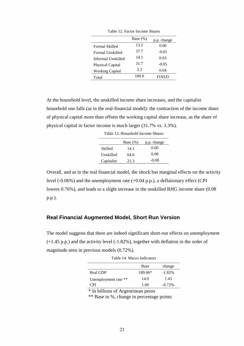
Table 12. Factor Income Shares

Base (%) p.p. change

Formal Skilled 13.2 0.00

Formal Unskilled 37.7 -0.01

Informal Unskilled 14.1 0.03

Physical Capital 31.7 -0.05

Working Capital 3.3 0.04

Total 100.0 FIXED

At the household level, the unskilled income share increases, and the capitalist

household one falls (as in the real-financial model): the contraction of the income share

of physical capital more than offsets the working capital share increase, as the share of

physical capital in factor income is much larger (31.7% vs. 3.3%).

Table 13. Household Income Shares

Base (%) p.p. change

Skilled 14.1 0.00

Unskilled 64.6 0.08

Capitalist 21.3 -0.08

Overall, and as in the real financial model, the shock has marginal effects on the activity

level (-0.06%) and the unemployment rate (+0.04 p.p.), a deflationary effect (CPI

lowers 0.76%), and leads to a slight increase in the unskilled RHG income share (0.08

p.p.).

Real Financial Augmented Model, Short Run Version

The model suggests that there are indeed significant short-run effects on unemployment

(+1.45 p.p.) and the activity level (-1.82%), together with deflation in the order of

magnitude seen in previous models (0.72%).

Table 14. Macro Indicators

Base change

Real GDP 189.86* -1.82%

Unemployment rate ** 14.0 1.45

CPI 1.00 -0.72%

* In billions of Argentinean pesos

** Base in %, change in percentage points

21

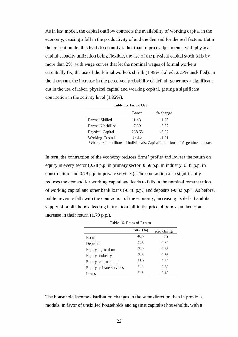
As in last model, the capital outflow contracts the availability of working capital in the

economy, causing a fall in the productivity of and the demand for the real factors. But in

the present model this leads to quantity rather than to price adjustments: with physical

capital capacity utilization being flexible, the use of the physical capital stock falls by

more than 2%; with wage curves that let the nominal wages of formal workers

essentially fix, the use of the formal workers shrink (1.95% skilled, 2.27% unskilled). In

the short run, the increase in the perceived probability of default generates a significant

cut in the use of labor, physical capital and working capital, getting a significant

contraction in the activity level (1.82%).

Table 15. Factor Use

Base* % change

Formal Skilled 1.43 -1.95

Formal Unskilled 7.39 -2.27

Physical Capital 288.65 -2.02

Working Capital 17.15 -1.91

*Workers in millions of individuals. Capital in billions of Argentinean pesos

In turn, the contraction of the economy reduces firms‟ profits and lowers the return on

equity in every sector (0.28 p.p. in primary sector, 0.66 p.p. in industry, 0.35 p.p. in

construction, and 0.78 p.p. in private services). The contraction also significantly

reduces the demand for working capital and leads to falls in the nominal remuneration

of working capital and other bank loans (-0.48 p.p.) and deposits (-0.32 p.p.). As before,

public revenue falls with the contraction of the economy, increasing its deficit and its

supply of public bonds, leading in turn to a fall in the price of bonds and hence an

increase in their return (1.79 p.p.).

Table 16. Rates of Return

Base (%) p.p. change

Bonds 48.7 1.79

Deposits 23.0 -0.32

Equity, agriculture 20.7 -0.28

Equity, industry 20.6 -0.66

Equity, construction 21.2 -0.35

Equity, private services 23.5 -0.78

Loans 35.0 -0.48

The household income distribution changes in the same direction than in previous

models, in favor of unskilled households and against capitalist households, with a

22

marginally higher intensity - the unskilled RHG increases and the capitalist RHG

decreases their income shares by 0.09 p.p. –as the negative hit on equity return earned

by capitalist households is larger.

Table 17. Household Income Shares

Base (%) p.p. change

Skilled 14.1 0.00

Unskilled 64.6 0.09

Capitalist 21.3 -0.09

The results in this model are diagrammed below (Diagram 4).

23

Diagram 4. Transmission channels for an increase in the perceived probability of default on domestic assets in the augmented short-run model

↑prob.of

domestic

default

(30 p.p.)

↑relative

return

of

foreign

assets

↑share of

foreign

assets in

households

portfolio

(0.28 p.p.)

↑ households

deposits

abroad

(2.91%)

↓ capital

account

balance

(16.6%)

↓ international

reserves (16.6%)

↑ trade

balance

(51.2%)

↑ exports

(2.96%)

↓ imports

(6.22%)

real depreciation,

with ↑ relative

price of tradables

(1.10%)

↓producer

prices

(0.70%)

↑ share of

tradables

in

value added

(0.26 p.p.)

↑ rel. wages

of formal

workers

(0.36% skilled,

0.62% unskilled)

↑ income share

of formal workers

(0.03 p.p. skilled,

0.05 p.p. unskilled)

↑ income share of

unskilled and ↓

share of capitalist

households (0.09 p.p.)

↓CPI

(0.72%)

↓use of formal workers

(1.95% skilled, 2.27%

unskilled)

& physical capital (2.02%)

↑rate of unemployment

(1.45 p.p.)

↓activity

level (1.82%)

↓public

revenue

(2.40%)

↓public

savings

(6.20%)

↑return

on public

bonds

(1.79 p.p.)

↑households

savings ↓households

consumption(3.64%)

↓ supply

of working

capital

(1.91%)

↑ real wage

of working

capital

(0.04%)

↑domestic

interest

rates

(0.32 p.p.

deposits,

0.48 p.p.

loans)

↑banks

holdings of

public bonds

(1.24%)

↑ current account

balance (16.6%)

24

5. Sensitivity analysis and model validation

With the double purpose of assessing the models robustness and validating the models

against econometric estimates, sensitivity analysis is done considering the same shock

but varying the import-domestic Armington, the export-domestic CET and the capitalist

household portfolio elasticity values.

Only the short-run model (RFAS) crashes in 1/3 of the solutions18

, suggesting the

possibility that the rigidities imposed in this model (the only difference with the RFA

model) may be making the model less robust to changes in elasticity parameters19

. In

the RFA model, increases in the elasticity of portfolio shares lead to a larger set of

capital outflows, needed real devaluations, and activity level contractions (as working

capital and the use of real factors fall). They also lead to larger increases in the share of

tradables in value added, and shift of the adjustment bulk from imports fall to exports

increase, as the scope to adjust is larger in the latter.

As expected, larger Armington and CET elasticity values reduce the size of the needed

devaluation. Increases in the Armington elasticity values shift the bulk of the needed

adjustment in the trade balance to imports contraction and ISI (import substitution

industrialization). As the CET elasticity increases, the bulk shifts to export expansion,

contracting the size of the industrial sector in the economy. The essential results are in

the following table, while the complete set of results extending the considered set of

elasticity values can be observed in Annex V.

18

With CET elasticity values of 0.5 and 1.01, and with portfolio elasticity values of 1.5 and 2. 19

This happened when starting from the initial solution. A change in the starting point of the solution may

avoid the commented crash.

25

Table 18. Sensitivity Analysis on real-financial-augmented (RFA) model

Relative deviations from base (%)*

* Except for shares where absolute deviations from base are reported

The elasticity of imports to changes in the real exchange rate coming out of the model

depends not only on the domestic-import Armington elasticity, but also on other

parameters (notably, the elasticity of household portfolio shares to changes in expected

returns). For the experiments performed, it is in the [1.01 - 4.15] interval. The values in

the interval exceed econometric estimates for the country during the Convertibility Plan:

Damill et al (2002,p38) reports an elasticity of 0.24420

, and Catao and Falcetti (2002) a

[0.7 – 0.8] range.

This could be indicating that the elasticity parameters in the model should be revised

downwards. However, the excess of the import elasticity coming from the model in

relation to econometrically estimated ones may be also due to the lack of use in the

mentioned regressions of a system of simultaneous equations which would have

accounted for the endogeneity of the variables explaining imports. Besides, it remains

unidentified which of the elasticity parameters present in the model should eventually

be revised, as different combinations of elasticity parameters would provide the model

with an import elasticity matching an econometrically estimated one.

6. Conclusions

The nested model elaborated here in the financial CGE framework allows looking at the

short and medium run effects of a large set of real and financial external shocks –

including those during the last globalization wave - on the levels of activity,

20

The regression controls for contemporaneous and (one-period) lagged real income.

ε=0.5 ε = 4.5 ε = 0.5 ε = 4.5 ε = 1.001 ε = 2.0

Capital Account NFPS -17.96 -17.44 -18.78 -17.44 -0.61 -610.83

Price of domestic goods -1.19 -0.78 -1.40 -0.78 -0.07 -25.65

Real GDP -0.06 -0.06 -0.04 -0.06 -0.01 -4.43

Tradables Value Added Shares

Primary 0.10 0.07 0.07 0.07 0.01 3.22

Industry 0.03 0.05 0.07 0.05 0.00 3.05

Elasticity respect to RER

Imports 1.01 4.12 4.11 4.12 4.15 2.87

Exports 3.60 3.31 0.63 3.31 3.15 5.27

CET elasticitiesHousehold portfolio

elasticity

Armington

elasticities

26

employment and income distribution in developing countries and throw light on the

transmission channels involved.

The model includes a series of features that characterize developing economies –

exogenous prices at which the economy can trade, presence of informal and segmented

labor markets, the existence of the working capital channel, etc. - and is easily adaptable

to different developing countries to the extent that they show a low degree of

sophistication in the financial markets21

.

The model captures the workings of the financial sphere and tracks the evolution of the

specific forms of savings and asset stocks, an essential part of the economic process

according to James Tobin (1981,p.13).

As suggested by the series of financial crisis hitting LDCs and the recent crisis

originated in developed countries with worldwide reverberation, the model includes a

critical transmission channel going from the financial to the real side of the economy:

the working capital channel in the “money in the production function” tradition started

by Milton Friedman (1969), where the availability of working capital hits the

productivity by which the real factors can be used and working capital acts, to a certain

extent, as a substitute for real factors. This intends to fill a gap found in financial CGE

models and is equivalent to the conventional relationship found in macroeconomic

models going from real supply of money to the activity level. The model includes a rich

variety of macroeconomic policy instruments, including detailed fiscal and monetary

instruments, orienting the model towards policy.

The model is applied in a static way to identify the short and medium run effects of an

increase in the perceived probability of default on domestic assets in Argentina during

the Currency Board regime. The model allows answering relevant questions like: 1)

how do expected defaults on domestic assets affect the economy? 2) are the short-run

effects very different to the middle-run ones?.

21

It the markets for public bonds and equity are absent, the adaptation simply consists in simplifying the

model.

27

The analysis illustrates that some financial shocks are out of the domain of applicability

of a non-financial model. When the financial dimension is accounted for but the

working capital channel is excluded, there are negligible effects on the economy. When

the working capital is included, if - as in Argentina -, the contribution of working capital

to value added is small, the effects in the medium run are also small. However, in the

short run, the effects on the level of activity and the rate of unemployment are

significant.

An increase in the perceived probability of default of 30 percentage points leads to

endogenous capital outflows that lower the international reserves held by the central

bank, the monetary aggregates and domestic credit, shifting the domestic interest rates

up and leading via a fall in the availability of working capital and in turn in the

productivity and use of the real factors to a contraction of the activity level of around

1.82% and an increase in the unemployment rate of around 1.45 percentage points. The

shock also leads to an improvement of the international investment position of the

country –with expansion of the foreign holdings of the non-financial private sector -,

and a consequent increase in the net investment income paid to residents. By generating

a real depreciation, capital outflows also lead to improve the country‟s trade deficit.

Paradoxically, the domestic firms financial constrains tighten in parallel to the domestic

private sector increasing its holdings of external assets, something observed in

Argentina. As the production structure of the economy changes, income distribution

changes - in the case of Argentina, capital outflows favor the unskilled and disfavor the

capitalist households.

Sensitivity analysis on the elasticity parameters was done to check the models

robustness and validate the model parameters against econometric estimates, and

showed that large shocks make the short-run version of the final model crash for a set of

elasticity parameters. The crashes, in turn, may be due to the difficulty of capturing

significant quantity adjustments in a model with neoclassical core. Besides, for the

model to account for the economic cycles generated by external shocks, it should be

made dynamic, which implies a detailed consideration of expectations formation. In the

process, the literature concerning models in the Keynesian tradition, including work by

Lance Taylor (2004) and Richard Agénor (2006) and New-Keynesian DSGE Models

such as Blanchard and Galí (2007) should be reviewed, identifying and implementing

28

needed model modifications. Once these changes are implemented, the parameters can

be adjusted to be consistent with parameter values estimated from a system of

simultaneous equations.

29

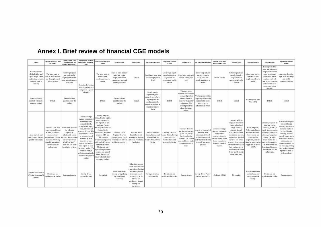
Annex I. Brief review of financial CGE models

Sphere Taylor (1981A) IS-LM in

the Tropics

Taylor (1981B) Ch8:

"Foreign Assets and

Balance of Payments"

(basic version)

Bourguignon, Branson

and De Melo "Maquette"

(1992)

Rosenzweig and Taylor

(1990) Easterly (1990) Lewis (1992) Decaluwe et al (1994)

Fargeix and Sadoulet

(1994)Yeldan (1997) Vos (1997) for Philipines

Adam & Bevan asset

market model (1998)Thissen (2000) Naastepad (2002) IMMPA (2003)

Agenor and Montiel

(2008)

Factors closures

(Default: labor and

capital wages are the

equilibrating variables

and only labor is

mobile)

The labor wage is

fixed or price-indexed

and the employment

level is flexible

Fixed wages (fixed

real mark-up for

capital) with flexible

labor use and capacity

utilization

The labor wage is

fixed and the

employment level is

flexible

Fixed or price-indexed

labor and capital

wages, with flexible

employment level and

capacity utilization

Default

Fixed labor wage with

flexible employment

level

Labor wage adjusts

partially through a

wage curve and

employment level is

flexible

Fixed labor wage with

flexible employment

level

Labor wage adjusts

partially through a

wage curve and

employment level is

flexible

Default closure

Labor wage adjusts

partially through a

wage curve and

employment level is

flexible

Labor wage is price-

indexed and the

employment level is

flexible

In a segment of the

labor market wages

are price-indexed or

move along wage

curves with flexible

employment level.

Land is fully employed

and immobile even

across agricultural

activities.

A version allows for

rigid labor real wage

and flexible

employment level

Products closures

(Default: prices are

market-clearing)

Default

Demand-driven

quantities clear the

markets

Default

Demand-driven

quantities clear the

markets

Default

Mostly quantity

adjustment given a

strong degree of price

rigidity (even the

producer price for

exports is fixed via an

equalization public

fund)

Default

Prices are set as

markups over variable

costs, and product

market closure is

achieved via quantity

adjustment. The

overall price level

clears the money

market.

"Fix-flex prices": Mark-

up pricing and quantity

adjustment in some

sectors, price

adjustment in others

Default Default Fix-flex prices (see

Vos 1997)Default Default

Asset markets and

their closures (Default:

quantity adjustment)

Deposits, loans from

households and banks

to firms, and banks

reserves. Asset

demands are in terms

of stocks. Working

capital is not rationed.

Interest rates are

endogenous.

Households demand

the following

imperfectly

substitutable assets:

deposits, foreign assets

and a non-tradable

("gold" or "land").

There are also loans

from banks to firms.

Money holdings

(against consolidated

financial system),

domestic bonds,

foreign bonds, equity,

loans, international

reserves. The portfolio

composition of assets

by households and

liabilities by firms

depends on asset

returns. The interest

rate adjusts to clear

the money market. The

return on equity is

endogenously given by

the return on physical

capital.

Currency, Deposits,

Loans, Bonds, Equity,

Loans provided by

and deposits of non-

residents, Foreign

Exchange Reserves of

Central Bank,

Rediscounts, Required

reserves. CES and

CET functions

determine composition

of household's assets

and firms liabilities.

The interest rate

adjusts to equate bank

sources and uses of

funds. The price of

equity adjusts to clear

the equity market.

Deposits, Loans,

Required Reserves,

Foreign Assets, Bonds

denominated in local

and foreign currency.

The core of the

financial system is

provided by deposits

and loans from banks.

See below.

Money, Deposits,

Loans, International

reserves held by

Central Bank, Bonds,

Equity.

Currency, Deposits,

Loans, Bonds, Foreign

currency held by

Central Bank and

households, Equity.

There are domestic

and foreign currency,

public and private

bonds and saving

deposits. The interest

rate equilibrates banks

sources and uses of

funds

A syste of "supply-led

finance (credit

rationing) with fixed

nominal returns and

perfectly elastic liability

demand" is at work

(p.333)

Currency holdings,

deposits in domestic

banks in local

currency, deposits

abroad, equity, bonds,

loans, international

reserves, required

reserves

Currency holdings,

deposits in domestic

banks in local and

foreign currency,

deposits abroad,

equity, bonds, loans,

international reserves,

rediscounts, required

reserves and excess

reserves. Asset returns

are calculated with ad-

hoc conditions, e.g.

interest rate on bonds

follow a uniform rate

of variation path.

Loans, Deposits,

Rediscounts, Bonds,

Required Reserves.

Asset returns are

determined by

regulation, with the

financial system being

supply-led as in Vos

(1997)

Currency, deposits (in

local and foreign

currency), bonds (in

middle-income country

version) and deposits

abroad, among other

assets. The public

bonds market has a

market-clearing price.

The interest rates on

deposits and loans are

linked to the rate on

rediscounts.

Currency holdings in

local and foreign

currency, deposits in

domestic banks in

local and foreign

currency, deposits

abroad, bonds, loans,

international reserves,

rediscounts, and

required reserves. At

the prevailing lending

rate, banks supply of

liquidity to firms is

perfectly elastic

Loanable funds market

("Saving-Investment")

closure

The interest rate

equilibrates the marketInvestment-driven

Savings-driven

(rationed credit)Not explicit

Investment-driven

(foreign savings being

the equilibrating

variable)

Either i) the interest

rate is fixed at a level

where planned savings

are below planned

investment (credit

rationing); or ii) the

interest rate

equilibrates planned

savings and

investments.

Savings-driven via

credit rationing

The interest rate

equilibrates the marketSavings-driven

Savings-driven ("prior-

savings approach")As Lewis (1992) Not explicit

Ex-post investment

function has a roof

given by available

savings

The interest rate

equilibrates the marketSavings-driven

Default or Keynesian

mark-up pricing with

endogenous capacity

utilization

30

Annex I. Review of financial CGE models (cont.)

Sphere Taylor (1981A) IS-LM in

the Tropics

Taylor (1981B) Ch8:

"Foreign Assets and

Balance of Payments"

(basic version)

Bourguignon, Branson

and De Melo "Maquette"

(1992)

Rosenzweig and Taylor

(1990) Easterly (1990) Lewis (1992) Decaluwe et al (1994)

Fargeix and Sadoulet

(1994)Yeldan (1997) Vos (1997) for Philipines

Adam & Bevan asset

market model (1998)Thissen (2000) Naastepad (2002) IMMPA (2003)

Agenor and Montiel

(2008)

Fiscal closure (Default:

flexible fiscal saving)Default

Fiscal institution is

absentDefault Default Default Default Default Default Default Default Default Default Default

Public transfers to

households are flexible

Fiscal institution is

absent

RoW closure 1:

exchange rate regime Fixed Crawling peg Fixed or flexible Fixed Fixed

Flexible (and other

schemes e.g. premium

rationing scheme for

imports)

Fixed Fixed or flexible Flexible Fixed Flexible Fixed FixedFixed, flexible or

administered Fixed or flexible

RoW closure 2:

balance of payments

With an omitted capital

account, foreign

reserves held by the

central bank change as

derived from the

endogenous trade

balance.

With an omitted capital

account, foreign

reserves held

domestically (by the

central bank and

households) change as

derived from the

endogenous trade

balance.

The balance of

payments is always in

equilibrium: in the fix

exchange rate regime,

government borrowing

equilibrates it

Endogenous trade

balance, capital

account balance and

overall balance

Endogenous trade

balance, capital

account balance

overall balance

Exogenous

international capital

flows determine the

capital account

balance and, with a

change in sign, the

current account

balance

Exogenous exports,

Armingtonian imports

and exogenous capital

account flows

determine the overall

result of the balance of

payments.

The current account,

the capital account (via

endogenous capital

flight) and the overall

result of the balance of

payments (in the fixed

exchange regime case)

are endogenous.

Exogenous (limited)

borrowing abroad by

private and public

sectors determine the

capital account

balance and, with a

change in sign, the

current account

balance

While capital flows are

exogenous and exports

are derived from CET

functions, imports

adjust to equilibrate

the balance of

payments.

Foreign savings are

exogenous

Endogenous current

account balance and

exogenous capital

flows reflecting limited

access to foreign

borrowing determine

the endogenous overall

result of the balance of

payments.

Exogenous capital

account, endogenous

current account and

overall result

Ilimited access by

banks to international

capital markets is

assumed to close their

gap between sources

and uses of funds, such

that the overall balance

of payments may end

in disequilibrium.

Residents are allowed

to exogenously hold

assets abroad, but non-

residents are not

allowed to hold

domestic assets

Intertemporal

equilibrium (Default:

single period without

role for expectations)

DefaultPerfect-foresight,

multiperiod model

Adaptive expectations,

multi-period modelMulti-period Default Default Default

Multi-period, adaptive

expectationsDefault Multiperiod Multi-period

Multi-period, average

of adaptive and

rational expectations

DefaultAdaptive expectations,

multiperiodDefault

Core links from

financial to real sphere

Depending on selected

parameters of saving

and investment

functions, monetary

contractions can either

lift or reduce the

activity level. Firms

borrow to finance

working capital needs,

but pass along the

financial costs without

effect on total output.

Financial credit chasing

producer's goods'

(p.152): excess supply

of loans leads to price

level increases that

lower the real interest

rate and lifts physical

investment

The interest rate

affects physical

investment. Also

working capital

channel

The interest rate

affects physical

investment

Real balances hit

consumption and firms

interest payments

affect their cash flow

and hence their

investment levels

The interest rate

affects real investment

and hence the

composition of

aggregate demand (not

the activity level,

determined by the full

employment

assumption). A

working capital

channel is also present.

Credit supply limits the

firms effective demand

for variable production

factors and physical

investment, with short

and medium run

effects.

Money emission leads

to inflation and real

wage fall, lifting labor

use and output. A

working capital

channel is also present

Money emission leads

to inflation and real

wage fall, lifting labor

use and output.

Exogenous capital

inflows may boost

investment

With full employment,

financial decisions (e.g.

public deficit bond-

financed vs money-

financed) may affect

output composition

The interest rate

affects real investment

Increasing the

availability of binding

working capital credit

(working capital being

a Leontief argument in

the production

function) allows to lift

firms product

A working capital

channel allows fall in

interest rates (via the

Central Bank reducing

the rediscount rate) to

reduce the effective

cost of labor,

estimulating labor use

and production

Same as IMMPA

(2003)

31

Annex II: Mathematical Statement of the Model

Real Sphere

Prices

Consumer Price Index

CPI =∑c

wcpic · PQc (1)

GDP Deflator

GDPDEFL =

∑a PV Aa ·QV Aa∑a PV A0a ·QV Aa

(2)

Price of imports by region

PMRc,r = pwmrc,r · (1 + tmrc,r) · exr c ∈ CM (3)

Price of imports

PMc ·QMc =∑r

PMRc,r ·QMRc,r c ∈ CM (4)

Price of exports by region

PERc,r = pwerc,r · (1− terc,r) · exr c ∈ CE (5)

Price of exports

PEc ·QEc =∑r

PERc,r ·QERc,r c ∈ CE (6)

Price of composite

PQc ·QQc = PDc ·QDc + PMc ·QMc (7)

32

Output price

PXc ·QXc = PDc ·QDc + PEc ·QEc (8)

Activity price

PAa =∑c

θa,c · PXACa,c (9)

Value added price

PAa ·QAa = PV Aa ·QV Aa + PINTAa ·QINTAa (10)

Aggregate intermediate price

PINTAa =∑c

icac,a · PQc (11)

Price of capital

PK =∑c

capcompc · PQc (12)

33

Production

Real Gross Domestic Product

RGDP =∑a

PV A0a ·QV Aa (13)

Leontief aggregate value added demand

QV Aa = ivaa ·QAa (14)

Leontief aggregate intermediate demand

QINTAa = intaa ·QAa (15)

CES aggregate value added

QV Aa = αvaa · (∑fa

δvafa,a ·QF−ρvaafa,a )

− 1ρvaa (16)

CES value added first order condition

Wfa ·WDISTfa,a = PV Aa · (1− tvaa) ·QV Aa · (17)∑fa′

(δvafa′,a ·QF−ρvaafa′,a )−1 · δvafa,a ·QF

−ρvaa −1fa,a

CES aggregate factors

QFfa,a = αgfa,a ·∑f

(δgf,fa,a ·QF−ρgfa,af,a )

− 1

ρgfa,a (18)

CES aggregate factors first order condition

Wf ·WDISTf,a =∑fa

(Wfa ·WDISTfa,a ·QFfa,a) (19)

·∑f ′,fa

(δgf ′,fa,a ·QF−ρgfa,af ′,a )−1

·∑fa

(δgf,fa,a ·QF−ρgfa,a−1f,a )

34

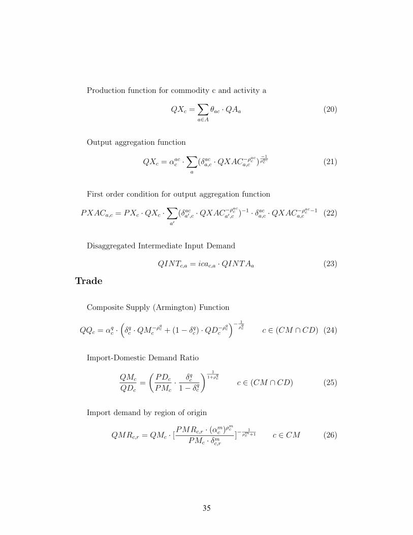
Production function for commodity c and activity a

QXc =∑a∈A

θac ·QAa (20)

Output aggregation function

QXc = αacc ·∑a

(δaca,c ·QXAC−ρacc

a,c )−1ρacc (21)

First order condition for output aggregation function

PXACa,c = PXc ·QXc ·∑a′

(δaca′,c ·QXAC−ρacca′,c )−1 · δaca,c ·QXAC−ρ

acc −1

a,c (22)

Disaggregated Intermediate Input Demand

QINTc,a = icac,a ·QINTAa (23)

Trade

Composite Supply (Armington) Function

QQc = αqc ·(δqc ·QM−ρqc

c + (1− δqc) ·QD−ρqc

c

)− 1

ρqc c ∈ (CM ∩ CD) (24)

Import-Domestic Demand Ratio

QMc

QDc

=

(PDc

PMc

· δqc1− δqc

) 1

1+ρqc

c ∈ (CM ∩ CD) (25)

Import demand by region of origin

QMRc,r = QMc · [PMRc,r · (αmc )ρ

mc

PMc · δmc,r]− 1ρmc +1 c ∈ CM (26)

35

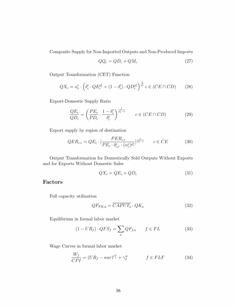
Composite Supply for Non-Imported Outputs and Non-Produced Imports

QQc = QDc +QMc (27)

Output Transformation (CET) Function

QXc = αtc ·(δtc ·QEρtc

c + (1− δtc) ·QDρtcc

) 1

ρtc c ∈ (CE ∩ CD) (28)

Export-Domestic Supply Ratio

QEcQDc

=

(PEcPDc

· 1− δtcδtc

) 1

ρtc−1

c ∈ (CE ∩ CD) (29)

Export supply by region of destination

QERc,r = QEc · [PERc,r

PEc · δec,r · (αec)ρec]

1ρec−1 c ∈ CE (30)

Output Transformation for Domestically Sold Outputs Without Exportsand for Exports Without Domestic Sales

QXc = QEc +QDc (31)

Factors

Full capacity utilization

QFFK,a = CAPUTa ·QKa (32)

Equilibrium in formal labor market

(1− URf ) ·QFSf =∑a

QFf,a f ∈ FL (33)

Wage Curves in formal labor market

Wf

CPI= (URf − nur)ε

wf + γwf f ∈ FLF (34)

36

Equilibrium in informal labor market

QFSFLIU =∑a

QFFLIU,a (35)

Unskilled factor supply allocation (formal vs. informal segments)∑flu

QFSflu = QFSFLUN (36)

Movement of unskilled to formal segment

QFSFLFU,t −QFSFLFU,t−1QFSFLIU,t

= εmigw · log(1− URFLFU,t) ·WFLFU,t

WFLIU,t

+ γmigw

(37)

Average wage

WAVf =Y Ff∑

aQF (f, a)(38)

Factor income

Y Ff =∑a

Wf ·WDISTf,a ·QFf,a (39)

Households

Household income

Y Hh =∑f

(shhfh,f · (1− tff ) · Y Ff ) + pedh ·∑e

DIV De (40)

+∑n

TRNSFRh,n +∑n

(FINTh,n − FINTn,h)

Household expenditure

EHh = Y Hh − SAVh (41)

37

Household Consumption Spending by Commodity

PQc ·QHc,h = PQc · γmc,h + βmc,h · (EHh −∑c′

(PQc′ · γmc′,h)) (42)

Enterprises

Before-Tax Profits

PROFBTe =∑a

WFK ·WDISTFK,a ·QFFK,a + FINTe,B − FINTB,e

+TRNSFRe,B (43)

Transfer of Banks Profits to Private Service Enterprises

TRNSFRES,B = PROFBTB (44)

Bank Profits

PROFBTB =∑n

(FINTB,n − FINTn,B) (45)

After-Tax Profits

PROFATe = min((1− tpre) ·PROFBTe, PROFBTe)+TRNSFRe,G (46)

Total Dividend Payments

DIV Te = max(0, shrpe · PROFATe) (47)

Dividend Payments to Residents

DIV De = SHEQDe ·DIV Te (48)

Dividend Payments to Non-Residents

DIV Ee = (1− SHEQDe) ·DIV Te (49)

38

Government

Government Revenue

Y G =∑f

tff · Y Ff +∑a

tvaa · PV Aa ·QV Aa (50)

+∑c,r

tmrc,r · pwmrc,r · exr ·QMRc,r

+∑c,r

terc,r · pwerc,r · exr ·QERc,r

+∑e

max(0, tpre · PROFBTe) +∑n

TRNSFRG,n

Central Bank Profits

PROFBTCB =∑n

(FINTCB,n − FINTn,CB) (51)

Transfer of Central Bank Profits to Central Government

TRNSFRG,CB = PROFBTCB (52)

Government Current Expenditures

EG =∑c

PQc ·QGCc +∑n

TRNSFRn,G +∑n

FINTn,G (53)

Savings

Household Savings

SAVh = mpsh ·MPSADJ · Y Hh (54)

Enterprise Savings

SAVe = PROFATe −DIV Te (55)

39

Government Savings

SAVG = Y G− EG (56)

Foreign Savings

SAVR = exr ·∑c,r

(pwmrc,r ·QMRc,r − pwerc,r ·QERc,r) (57)

+∑e

DIV Ee +∑n

FINTR,n −∑n

FINTn,R

+∑n

(TRNSFRR,n − TRNSFRn,R)

Total Savings

SAV TOT =∑n

SAVn (58)

Investment

Total investment value

V IT =∑a

V Ia (59)

Investment value by sector

V Ia = PK ·∆QKa (60)

Gross variation in quantity of capital by sector

∆QKa = dqkna · [WFK ·WDISTFK,a

RL · PK]εIq a ∈ APRI (61)

Investment demand by sector of origin

QIc = capcompc ·∑a

∆QKa (62)

40

Savings-Investment Balance

V IT = SAV TOT +WALRAS (63)

Equilibria in commodity markets

QQc =∑a

QINTc,a +∑h

QHc,h +QIc +QGCc (64)

Updating condition for physical capital

QFFK,a,t = (1− δk) ·QFFK,a,t−1 + ∆QKa,t−1 (65)

Balance of Payments I

Variation in International Reserves

∆INTRES = CAB +KAB (66)

Current Account Balance

exr · CAB = −SAVR (67)

Capital Account Balance

exr ·KAB =∑e

(∆EQEe) + ∆DEPR + ∆V BONDR (68)

−exr∑da

∆DEPAda

Financial Sphere

41

Households portfolio

Household Portfolio Balance

CURRh +DEPh + exr ·DEPDh + AHh = LOANh +NFWh (69)

Allocation of Currency Supply Among Households

CURRS =∑h

CURRh (70)

Demand for dolar-denominated domestic deposits by Profit-Earner House-hold

exr ·DEPDHC = DEPHC (71)

Demand for Bonds by Profit-Earner Household

PBOND ·BONDHC = ΘHCG · AHHC (72)

Demand for Equity by Profit-Earner Household

EQDe = ΘHCe · AHHC (73)

Demand for Deposits Abroad by Profit-Earner Household

DEPAHC = ΘHCR · AHHC (74)

Share of Bonds in Capitalist Household Portfolio

ΘHCG =

(δHCG )εHC · (RB · (1− pdefHC,G))εHC−1

QHC(75)

Share of Equity in Capitalist Household Portfolio

ΘHCe =

(δHCe )εHC · (REe)εHC−1

QHC(76)

42

Share of Deposits Abroad in Capitalist Household Portfolio

ΘHCR =

(δHCR )εHC · (RW · (1− pdefHC,R))εHC−1

QHC(77)

Harmonic Mean for Capitalist Household Portfolio Shares

QHC = (δHCG )εHC · (RB · (1− pdefHC,G))εHC−1 (78)

+∑e

(δHCe )εHC · (REe)εHC−1

+(δHCR )εHC · (RW · (1− pdefHC,R))εHC−1

Enterprise balance equation

DEPe = LOANe + EQTe +NFWe (79)

Equity composition

EQTe = EQDe + EQEe (80)

Residents Share in Equity

SHEQDe =EQDe

EQTe(81)

Government portfolio

Bonds Emission

PBOND ·∆BONDS =∑c

PQc ·∆QKAG − SAVG (82)

Bank portfolio

Banks portfolio balance

AB +REQRES =∑dd

(DEPdd + exr ·DEPDdd) +RED +NFWB (83)

43

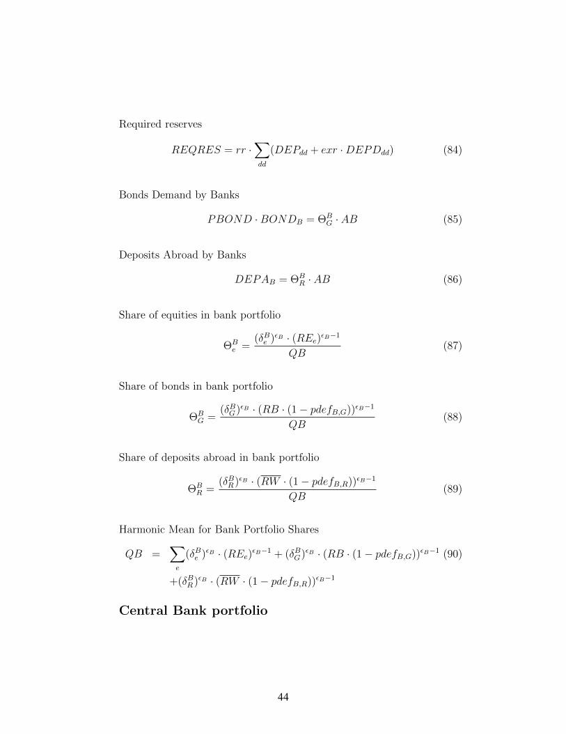
Required reserves

REQRES = rr ·∑dd

(DEPdd + exr ·DEPDdd) (84)

Bonds Demand by Banks

PBOND ·BONDB = ΘBG · AB (85)

Deposits Abroad by Banks

DEPAB = ΘBR · AB (86)

Share of equities in bank portfolio

ΘBe =

(δBe )εB · (REe)εB−1

QB(87)

Share of bonds in bank portfolio

ΘBG =

(δBG)εB · (RB · (1− pdefB,G))εB−1

QB(88)

Share of deposits abroad in bank portfolio

ΘBR =

(δBR)εB · (RW · (1− pdefB,R))εB−1

QB(89)

Harmonic Mean for Bank Portfolio Shares

QB =∑e

(δBe )εB · (REe)εB−1 + (δBG)εB · (RB · (1− pdefB,G))εB−1 (90)

+(δBR)εB · (RW · (1− pdefB,R))εB−1

Central Bank portfolio

44

Central Bank Portfolio Balance

exr · INTRES + PBOND ·BONDCB +RED = MB +NFWCB (91)

Rates of return

Rate of interest on domestic banks loans

RL =RD

1− rr· (1 + µ) (92)

Bonds demand-supply equilibrium

BONDS =∑b

(BONDb) (93)

Rate of return on bonds

RB =1

PBOND·RB0 (94)

Rate of return on enterprise equity

REe =PROFATeEQTe

(95)

Interest payments

Interest flows on deposits

FINTdd,B = RD · (DEPdd + exr ·DEPDdd) (96)

Interest flows on loans

FINTB,l = RL · LOANl (97)

Interest flows on bonds

FINTb,G = RB · PBOND ·BONDb (98)

45

Interest flows on deposits abroad

FINTda,R = RW · exr ·DEPAda (99)

Interest flows on central bank’ international reserves

FINTCB,R = RW · exr · INTRES (100)

Interest flows on rediscounts

FINTCB,B = RRED ·RED (101)

Balance of Payments II

Variation of international reserves as a function of capital account balance

∆INTRES = flexibir ·KAB (102)

Monetary Base Constrain

CURRS +REQRES = MB (103)

Updating conditions for financial stocks

Households net financial wealth

∆NFWh,t = SAVh,t (104)

Firms net financial wealth

∆NFWe,t = SAVe,t − V Ia,t (105)

Bonds supply

BONDSt = BONDSt−1 + ∆BONDSt (106)

46

Bonds by holder

BONDn,t = BONDn,t−1 + ∆BONDn,t (107)

Bond value by holder

∆V BONDn,t = PBONDt ·BONDn,t − PBONDt−1 ·BONDn,t−1 (108)

International reserves

INTRESt = INTRESt−1 + ∆INTRESt (109)

Deposits of non-residents

DEPR,t = DEPR,t−1 + ∆DEPR,t (110)

Equity Held by Non-Residents

EQEe,t = EQEe,t−1 + ∆EQEe,t (111)

Deposits abroad

DEPAda,t = DEPAda,t−1 + ∆DEPAda,t (112)

Money out of the production function

Loans Supply by Banks

LOANl = ΘBl · AB l ∈ L (113)

Liquidity preference - money supply equilibrium

logMB

GDPDEFL= εmy · log(RGDP )− εmr · log(RD) + γLM (114)

47

Money in the production function

Working capital supply

QFSFW =LOANE

GDPDEFL(115)

Equilibrium in working capital market

(1− URW ) ·QFSFW =∑fw,a

QFfw,a (116)

Bank loans supply at aggregated level

LOANE =∑e

ΘBe · AB (117)

Bank loans supply at disaggregated level

LOANe =QFFW,aQFSFW

· LOANE (118)

Average wage for working capital

WAVFW =Y FFWQFSFW

(119)

Minimum average wage for working capital

WAVFW ≥ minwwk (120)

Liquidity preference - money supply equilibrium

RL = WAVFW ·GDPDEFL (121)

48

Sets

Name Definitiona Activities

apri Private Activitiesb Bond Holdersc Commodities

cdc Commodities Demanded Domesticallycec Commodities Exportedcmc Commodities Importedcxc Commodities Produced Domesticallyda Deposits Abroad Holdersdd Domestic Deposits Holderse Enterprisesf Factors

faf Factor Aggregatesfbf Factors at Bottom of Production Functionflff Formal Labor Factorfluf Unskilled Labor Factorfwf Uses of working capital in the production functionh Households

hsu Skilled and Unskilled Householdsl Loan Holders with firms disaggregated

lb Loan Holders with firms aggregatedn Institutionsr Regionst Time set

49

Elements of sets referred in model equations

Name DefinitionAG Public ActivityB Commercial Banks

CB Central BankE Enterprise (supra-sector)ES Private Services EnterprisesFK Physical Capital Factor

FLFU Formal Unskilled LaborFLIU Informal Unskilled LaborFLUN Unskilled LaborFW Working Capital FactorG Government

HC Capitalist HouseholdR Rest-of-world

50

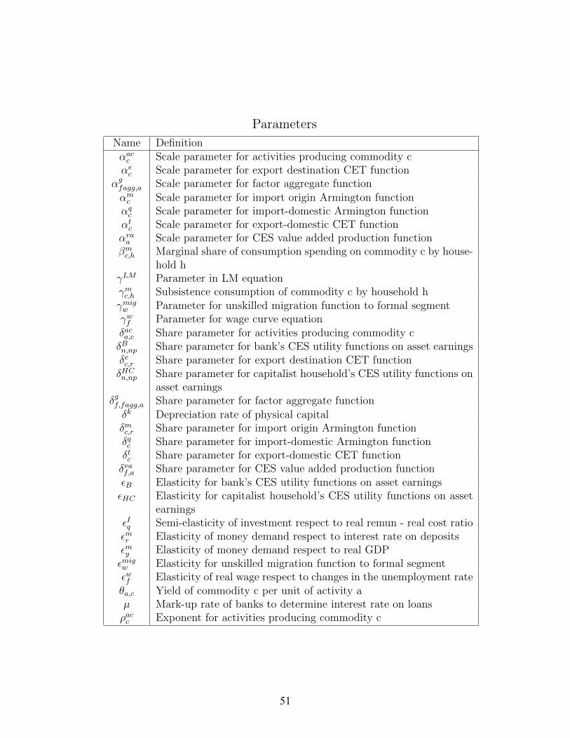
Parameters

Name Definitionαacc Scale parameter for activities producing commodity cαec Scale parameter for export destination CET function

αgfagg,a Scale parameter for factor aggregate function

αmc Scale parameter for import origin Armington functionαqc Scale parameter for import-domestic Armington functionαtc Scale parameter for export-domestic CET functionαvaa Scale parameter for CES value added production functionβmc,h Marginal share of consumption spending on commodity c by house-

hold hγLM Parameter in LM equationγmc,h Subsistence consumption of commodity c by household hγmigw Parameter for unskilled migration function to formal segmentγwf Parameter for wage curve equationδaca,c Share parameter for activities producing commodity cδBn,np Share parameter for bank’s CES utility functions on asset earningsδec,r Share parameter for export destination CET functionδHCn,np Share parameter for capitalist household’s CES utility functions on

asset earningsδgf,fagg,a Share parameter for factor aggregate function

δk Depreciation rate of physical capitalδmc,r Share parameter for import origin Armington functionδqc Share parameter for import-domestic Armington functionδtc Share parameter for export-domestic CET functionδvaf,a Share parameter for CES value added production functionεB Elasticity for bank’s CES utility functions on asset earningsεHC Elasticity for capitalist household’s CES utility functions on asset

earningsεIq Semi-elasticity of investment respect to real remun - real cost ratioεmr Elasticity of money demand respect to interest rate on depositsεmy Elasticity of money demand respect to real GDPεmigw Elasticity for unskilled migration function to formal segmentεwf Elasticity of real wage respect to changes in the unemployment rateθa,c Yield of commodity c per unit of activity aµ Mark-up rate of banks to determine interest rate on loansρacc Exponent for activities producing commodity c

51

Parameters (cont)

Name Definitionρec Exponent for export destination CET function

ρgfagg,a Exponent for factor aggregate function

ρmc Exponent for import origin Armington functionρqc Exponent for import-domestic Armington functionρtc Exponent for export-domestic CET functionρvaa Exponent for CES value added production function

capcompc Share of good c in composition of capital gooddqkna Parameter for investment function

exr Nominal exchange rate - local currency units per USD -flexibir Sensibility of the balance of payment result to the capital account

balanceicac,a Intermediate input c per unit of aggregate intermediate of act. aintaa Aggregate intermediate input coefficientivaa Aggregate value added coefficient

minwwk Minimum average wage of working capitalmpsh Initial marginal propensity to save for householdsnur Natural unemployment rate

pdefn,n′ Probability of default perceived by inst n about inst n’ paymentspedh Capitalist households dummy (1 for capitalist, 0 otherwise)

pwerc,r World price of export by commodity and region - in dollarspwmrc,r World price of imports by region - in dollars

rr Cash reserve ratio on bank depositsshhfh,f Share of household h in factor f incomeshrpn Share of profits retained by enterprise nterc,r Rate of tax on exports by region and sectortff Rate of direct tax on factors (social security tax)

tmrc,r Rate of tax on imports by region and sectortprn Rate of tax to profitstvaa Rate of VATwcpic CPI weights

52

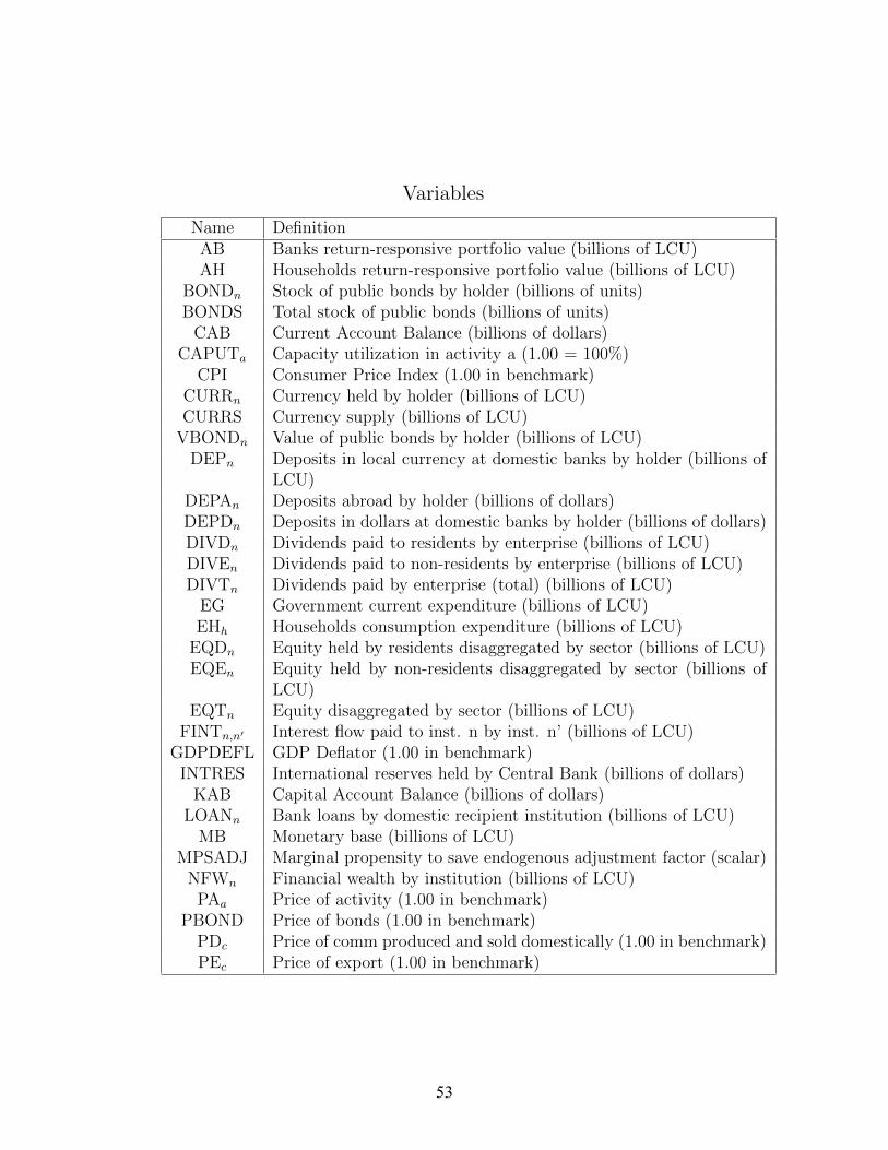
Variables

Name DefinitionAB Banks return-responsive portfolio value (billions of LCU)AH Households return-responsive portfolio value (billions of LCU)

BONDn Stock of public bonds by holder (billions of units)BONDS Total stock of public bonds (billions of units)

CAB Current Account Balance (billions of dollars)CAPUTa Capacity utilization in activity a (1.00 = 100%)

CPI Consumer Price Index (1.00 in benchmark)CURRn Currency held by holder (billions of LCU)CURRS Currency supply (billions of LCU)

VBONDn Value of public bonds by holder (billions of LCU)DEPn Deposits in local currency at domestic banks by holder (billions of

LCU)DEPAn Deposits abroad by holder (billions of dollars)DEPDn Deposits in dollars at domestic banks by holder (billions of dollars)DIVDn Dividends paid to residents by enterprise (billions of LCU)DIVEn Dividends paid to non-residents by enterprise (billions of LCU)DIVTn Dividends paid by enterprise (total) (billions of LCU)

EG Government current expenditure (billions of LCU)EHh Households consumption expenditure (billions of LCU)

EQDn Equity held by residents disaggregated by sector (billions of LCU)EQEn Equity held by non-residents disaggregated by sector (billions of

LCU)EQTn Equity disaggregated by sector (billions of LCU)

FINTn,n′ Interest flow paid to inst. n by inst. n’ (billions of LCU)GDPDEFL GDP Deflator (1.00 in benchmark)

INTRES International reserves held by Central Bank (billions of dollars)KAB Capital Account Balance (billions of dollars)

LOANn Bank loans by domestic recipient institution (billions of LCU)MB Monetary base (billions of LCU)

MPSADJ Marginal propensity to save endogenous adjustment factor (scalar)NFWn Financial wealth by institution (billions of LCU)

PAa Price of activity (1.00 in benchmark)PBOND Price of bonds (1.00 in benchmark)

PDc Price of comm produced and sold domestically (1.00 in benchmark)PEc Price of export (1.00 in benchmark)

53

Variables (cont.)

Name DefinitionPERc,r Price of export by region of destination (1.00 in benchmark)

PINTAa Price of intermediate aggregate (1.00 in benchmark)PK Price of capital (1.00 in benchmark)PMc Price of import (1.00 in benchmark)

PMRc,r Price of import by region of origin (1.00 in benchmark)PQc Price of composite good (1.00 in benchmark)

PROFATn After-tax profits (billions of LCU)PROFBTn Before-tax profits (billions of LCU)

PVAa Price of value added (1.00 in benchmark)PXc Average output price (1.00 in benchmark)

PXACa,c Price of commodity c generated by activity a (1.00 in benchmark)QAa Domestic output by activity (billions of units)QB Harmonic mean in financial CES utility function of banksQDc Quantity of domestic sales (billions of units)QEc Quantity of exports (billions of units)

QERc,r Quantity of exports to region r (billions of units)QFf,a Quantity of factor f employed in act a (billions of units)QFSf Quantity of factor f supply (billions of units)QGCc Quantity of public consumption of comm c (billions of units)QHc,h Quantity of comm c consumed by household h (billions of units)QHC Harmonic mean in financial CES utility function of capitalist house-

holdsQIc Quantity of private investment by sector of origin (billions of units)

QINTc,a Quantity of intermediate input c used by activity a (billions ofunits)

QINTAa Quantity of intermediate inputs used by activity a (billions of units)QKa Physical capital stock in activity a (billions of units)QMc Quantity of imports (billions of units)

QMRc,r Quantity of imports from region r (billions of units)QHP Harmonic mean in financial CES utility function of capitalist house-

hold (billions of units)QQc Quantity of composite good c (billions of units)

QVAa Quantity of value added demanded by act a -gross of VAT andfactor taxes (billions of units)

QXc Quantity of commodity output (billions of units)

54

Variables (cont.)

Name DefinitionQXACa,c Quantity of commodity output by activity (billions of units)

RB Rate of interest on public bonds (1.00 = 100%)RD Rate of interest on deposits at domestic banks (1.00 = 100%)REe Rate of return on enterprise equity, by enterprise (1.00 = 100%)RED Central Bank rediscount level (billions of LCU)

REQRES Required bank reserves (billions of LCU)RGDP Real GDP (billions of units)

RL Rate of interest on domestic banks loans (1.00 = 100%)RRED Rate of interest on Central Bank rediscounts (1.00 = 100%)

RW Risk-free world interest rate (1.00 = 100%)SAVn Savings by institution (billions of LCU)

SAVTOT Total savings (billions of LCU)SHEQDn Share of residents in equity (1.00 = 100%)

ΘBn Shares of financial assets in banks portfolio (1.00 = 100%)

ΘHPn Shares of financial assets in capitalist household portfolio (1.00 =

100%)TRNSFRn,n′ Transfer to institution n by institution n’ (billions of LCU)

URf Unemployment rate of factor f (1.00 = 100%)URW Unemployment rate of working capital (1.00 = 100%)VIa Value of investment by sector of destination (billions of LCU)VIT Value of total investment (billions of LCU)Wf Nominal wage for factor f before factor tax payment and distorsions

(thousands of LCU)WALRAS Walras variable -0 if agg savings = agg investment-

WAVf Average nominal wage for factor f before factor tax payment ac-counting for distorsions (thousands of LCU)

WDISTf,a Factor wage distorsion for factor f in activity a (scalar)YFf Total factor income before taxes to factors by factor (billions of

LCU)YG Total government income (billions of LCU)YHh Total household income after interest flow by household (billions of

LCU)

55

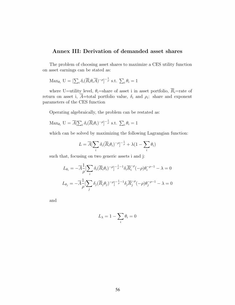
Annex III: Derivation of demanded asset shares

The problem of choosing asset shares to maximize a CES utility functionon asset earnings can be stated as:

Maxθi U = [∑

i δi(RiθiA)−ρ]−1ρ s.t.

∑i θi = 1

where U=utility level, θi=share of asset i in asset portfolio, Ri=rate ofreturn on asset i, A=total portfolio value, δi and ρi: share and exponentparameters of the CES function

Operating algebraically, the problem can be restated as:

Maxθi U = A[∑

i δi(Riθi)−ρ]−

1ρ s.t.

∑i θi = 1

which can be solved by maximizing the following Lagrangian function:

L = A[∑i

δi(Riθi)−ρ]−

1ρ + λ(1 −

∑i

θi)

such that, focusing on two generic assets i and j:

Lθi = −A1

ρ[∑i

δi(Riθi)−ρ]−

1ρ−1δiR

−ρi (−ρ)θ−ρ−1

i − λ = 0

Lθj = −A1

ρ[∑j

δj(Rjθj)−ρ]−

1ρ−1δjR

−ρj (−ρ)θ−ρ−1

j − λ = 0

and

Lλ = 1 −∑i

θi = 0

56

From the Lθi = 0 and Lθj = 0 conditions,

δiR−ρi θ−ρ−1

i = δjR−ρj θ−ρ−1

j

Isolating θj,

θj = θiδ− 1ρ+1

i Rρρ+1

i δ1ρ+1

j R− ρρ+1

j

Given that in a CES function the elasticity ε = 1ρ+1

,

θj = θiδ−εi R

1−εi δεjR

ε−1

j

And, given that the sum of the asset shares equals one, i.e.∑

j θj = 1:

∑j

θj =∑j

(θiδ−εi R

1−εi δεjR

ε−1

j ) = 1

Taking common factor θiδ−εi R

1−εi ,

θiδ−εi R

1−εi

∑j

δεjRε−1

j = 1

And, operating conveniently, we get to the final formula which determinesthe asset shares given the CES function parameters and the assets returns,where ε should exceed 1:

θi =δεiR

ε−1

i∑j δ

εjR

ε−1

j

57

Annex IV. Results of additional external shocks

+:increases; ++: increases by more than 0.3% (p.p. for ratios); -: falls; --: falls by more than 0.3% (p.p. for ratios)

∆ In the balance of payments, following national accounts system, a + (-) means that the flow leads country's international reserves holdings to

increase (fall)

R RF RFA R RF RFA R RF RFA R RF RFA R RF RFA R RF RFA R RF RFA R RF RFA R RF RFA R RF RFA

Balance of Payments∆

Current Account ++ ++ ++ ++ ++ ++ ++ ++ ++ ++ -- -- -- ++ ++ + - -- - -- -- -- --

Trade Balance ++ ++ -- -- -- ++ ++ ++ ++ ++ ++ -- -- -- - ++ ++ + ++ ++ -- -- -- ++ -- -- -- -- --

Exports of Goods and NFS ++ ++ -- -- -- ++ ++ ++ ++ ++ ++ -- -- -- ++ ++ ++ ++ ++ ++ ++ ++ ++ ++ ++ ++ -- -- --

Imports of Goods and NFS -- -- ++ ++ ++ -- -- -- -- -- -- ++ ++ ++ ++ ++ ++ ++ ++ ++ ++ ++ ++ ++ ++ ++ ++ ++ ++

Investment Income - - ++ ++ ++ + ++ ++ + -- -- - - - + -- -- - - -- + ++ ++ -- ++ ++ ++ ++ ++

Interests - - ++ ++ ++ ++ ++ -- -- + + -- -- - -- ++ ++ ++ ++ ++ ++ ++

Profits and Dividends + + -- -- -- ++ ++ ++ ++ ++ ++ -- -- -- + + + - - - ++ ++ ++ -- -- -- -- -- --

Capital Account -- -- -- -- -- -- -- -- -- -- ++ ++ ++ -- -- - + ++ + ++ ++ ++ ++

Non Financial Private Sector -- -- -- -- -- -- -- -- -- ++ ++ -- -- - + ++ + ++ ++ ++ ++

Public Sector FX FX FX FX FX FX FX FX FX FX FX ++ ++ ++ FX FX FX FX FX FX FX FX FX FX FX FX FX FX FX

Commercial Banks + + -- -- -- -- -- ++ ++ -- -- + + + + -- -- -- -- -- --

Public Deficit ++ ++ -- -- -- + ++ ++ ++ ++ ++ -- -- -- ++ ++ ++ + ++ ++ -- -- -- -- -- -- -- -- --

Price of domestic goods - - ++ ++ ++ -- -- -- -- -- -- ++ ++ ++ - -- -- + + + -- -- -- ++ ++ ++ ++ ++ ++

Real GDP - - + + - - - - - - - + + + + + + + + + ++ ++ ++ ++ ++ + + + +

Factor use

Formal Skilled - - + + - - - - - - - + + + + + + + + + + + + + + + + + +

Formal Unskilled - - + + - - - - - - - + + + + + + + + + ++ ++ ++ ++ ++ ++ + + ++

Physical Capital

Working Capital -- -- -- -- ++ + - ++ -- ++

Tradables Value Added Shares

Agriculture + + -- -- -- + + + + + + - - - + + + - - - + + + + + + - -- --

Industry + + -- - - + + + + + + - - - + + + + + + - - - - - - - -- --

Real Wages

Formal Skilled - - + + - - - - - - - + + + + + + + + + ++ ++ ++ ++ ++ ++ + + ++

Formal Unskilled - - + + - - - - - - - + + + + + + + + + ++ ++ ++ ++ ++ ++ + + +

Informal Unskilled + + -- -- -- + + + + + + -- -- -- + + + + + + ++ ++ ++ ++ ++ ++ - -- --

Physical Capital - - + + -- - - - - - - + + ++ + + + + + + ++ ++ ++ ++ ++ ++ + ++ ++

Working Capital ++ ++ ++ ++ -- - ++ -- ++ --

Factor Income Shares

Formal Skilled - - + + + - - - - - - + + + - - - - - - - - - - - - + + +

Formal Unskilled - - + + + - - - - - - + + + - - - + + + - - - - - + + + +

Informal Unskilled + + - - - + + + + + + - - - + + + - - - + + + + + - - - -

Physical Capital - - + + - - - - - - - + + + + + + + + - + + + + + - + + +

Working Capital + + + + - - + - + -

Household Income Shares

Skilled - - -- -- -- - - - - - - + + + - - - + + + - - - + + + + + +

Unskilled + + -- -- -- + - - + + + - - - + - - - - - + + - + - - - -- --

Capitalist - - ++ ++ ++ + + + + - - - + + + + + - + + + + + - - + - ++ ++

Rate of tax on

exports ↓10%

Price of exports

↑10%

Price of imports

↓10%

Nominal

exchange rate

↑10%

Perceived prob

of default on

domestic assets

↑10 p.p.

Risk-free world

interest rate

↑10 p.p.

Deposits held by

non-residents

↓10%

Equity held by

non-residents

↓10%

Bonds held by

non-residents

↑10%

Rate of tax on

imports ↓10%

58

Annex V. Results of sensitivity analysis

Table. Sensitivity Analysis on import-domestic origin Armington elasticities

increasing 30% the perceived probability of default on domestic assets

Relative deviations from base (%) *

* Except for shares, where absolute deviations from base are reported

∆ In the balance of payments, following national accounts system, a + (-) means that the

flow leads country's international reserves holdings to increase (fall)

Amount Unit ε = 0.5 ε = 1.001 ε = 2.25 ε = 4.5

Balance of Payments∆

Current Account -8.46 B$ 12.63 12.56 12.42 12.27

Trade Balance 3.44 B$ 32.92 32.95 33.00 33.05

Exports of Goods and NFS 21.51 B$ 4.26 3.93 3.30 2.58

Imports of Goods and NFS 18.07 B$ -1.20 -1.60 -2.36 -3.22

Investment Income -11.90 B$ -0.54 -0.60 -0.71 -0.84

Interests -10.91 B$ -0.70 -0.76 -0.86 -0.99

Profits and Dividends -0.99 B$ 1.19 1.12 0.97 0.81

Current Transfers FIXED FIXED FIXED FIXED

Capital Account 10.62 B$ -12.63 -12.56 -12.42 -12.27

Non Financial Private Sector 7.50 B$ -17.96 -17.86 -17.67 -17.44

Public Sector 1.99 B$ FIXED FIXED FIXED FIXED

Commercial Banks 1.13 B$ 0.60 0.59 0.57 0.55

Public Deficit 11.99 B$ 1.17 1.19 1.21 1.24

Price of domestic goods 1.00 $ -1.19 -1.11 -0.95 -0.78

Real GDP 189.86 B$ -0.06 -0.06 -0.06 -0.06

Factor use

Formal Skilled 1.43 mill. indiv -0.03 -0.03 -0.03 -0.03

Formal Unskilled 7.39 mill. indiv -0.06 -0.06 -0.06 -0.06

Working Capital 17.15 B$ -0.87 -0.93 -1.04 -1.16

Tradables Value Added Shares

Agriculture 10.9 % 0.10 0.09 0.08 0.07

Industry 25.8 % 0.03 0.03 0.04 0.05

Real Wages

Formal Skilled 16.82 th$/indiv -0.06 -0.06 -0.06 -0.06

Formal Unskilled 9.29 th$/indiv -0.03 -0.03 -0.03 -0.03

Informal Unskilled 9.29 th$/indiv 0.29 0.26 0.21 0.15

Physical Capital 0.20 % of stock v. -0.13 -0.14 -0.17 -0.19

Working Capital 0.35 % of stock v. 1.74 1.84 2.05 2.28

Factor Income Shares

Formal Skilled 13.2 % -0.01 -0.01 -0.01 0.00

Formal Unskilled 37.7 % -0.03 -0.03 -0.02 -0.01

Informal Unskilled 14.1 % 0.04 0.04 0.03 0.03

Physical Capital 31.7 % -0.04 -0.04 -0.04 -0.05

Working Capital 3.3 % 0.03 0.03 0.03 0.04

Household Income Shares

Skilled 14.1 % -0.01 -0.01 -0.01 0.00

Unskilled 64.6 % 0.08 0.08 0.08 0.08

Capitalist 21.3 % -0.07 -0.07 -0.07 -0.08

Elasticity of imports r.t. RER 1.01 1.44 2.47 4.12

Base ↑PDEF by 30%

59

Table. Sensitivity Analysis on export-domestic destination CET elasticities

increasing 30% the perceived probability of default on domestic assets

Relative deviations from base (%)*

* Except for shares, where absolute deviations from base are reported

∆ In the balance of payments, following national accounts system, a + (-) means that the

flow leads country's international reserves holdings to increase (fall)

Amount Unit ε = 0.5 ε = 1.001 ε = 2.25 ε = 4.5

Balance of Payments∆

Current Account -8.46 B$ 13.18 12.97 12.62 12.27

Trade Balance 3.44 B$ 35.83 35.19 34.12 33.05

Exports of Goods and NFS 21.51 B$ 0.89 1.29 1.95 2.58

Imports of Goods and NFS 18.07 B$ -5.76 -5.16 -4.18 -3.22

Investment Income -11.90 B$ -0.99 -0.96 -0.90 -0.84

Interests -10.91 B$ -1.21 -1.16 -1.07 -0.99

Profits and Dividends -0.99 B$ 1.37 1.24 1.02 0.81

Current Transfers FIXED FIXED FIXED FIXED

Capital Account 10.62 B$ -13.18 -12.97 -12.62 -12.27

Non Financial Private Sector 7.50 B$ -18.78 -18.47 -17.95 -17.44

Public Sector 1.99 B$ FIXED FIXED FIXED FIXED

Commercial Banks 1.13 B$ 0.84 0.77 0.66 0.55

Public Deficit 11.99 B$ 2.18 1.97 1.60 1.24

Price of domestic goods 1.00 $ -1.40 -1.25 -1.01 -0.78

Real GDP 189.86 B$ -0.04 -0.05 -0.06 -0.06

Factor use

Formal Skilled 1.43 mill. indiv -0.02 -0.02 -0.02 -0.03

Formal Unskilled 7.39 mill. indiv -0.03 -0.04 -0.05 -0.06

Working Capital 17.15 B$ -0.78 -0.87 -1.02 -1.16

Tradables Value Added Shares

Agriculture 10.9 % 0.07 0.07 0.07 0.07

Industry 25.8 % 0.07 0.06 0.06 0.05

Real Wages

Formal Skilled 16.82 th$/indiv -0.04 -0.05 -0.05 -0.06

Formal Unskilled 9.29 th$/indiv -0.02 -0.02 -0.03 -0.03

Informal Unskilled 9.29 th$/indiv 0.20 0.20 0.18 0.15

Physical Capital 0.20 % of stock v. -0.08 -0.11 -0.15 -0.19

Working Capital 0.35 % of stock v. 1.60 1.76 2.02 2.28

Factor Income Shares

Formal Skilled 13.2 % -0.01 -0.01 -0.01 0.00

Formal Unskilled 37.7 % -0.02 -0.02 -0.02 -0.01

Informal Unskilled 14.1 % 0.03 0.03 0.03 0.03

Physical Capital 31.7 % -0.03 -0.03 -0.04 -0.05

Working Capital 3.3 % 0.03 0.03 0.03 0.04

Household Income Shares

Skilled 14.1 % -0.02 -0.01 -0.01 0.00

Unskilled 64.6 % 0.07 0.07 0.08 0.08

Capitalist 21.3 % -0.06 -0.06 -0.07 -0.08

Elasticity of imports r.t. RER 4.11 4.12 4.12 4.12

Base ↑PDEF by 30%

60

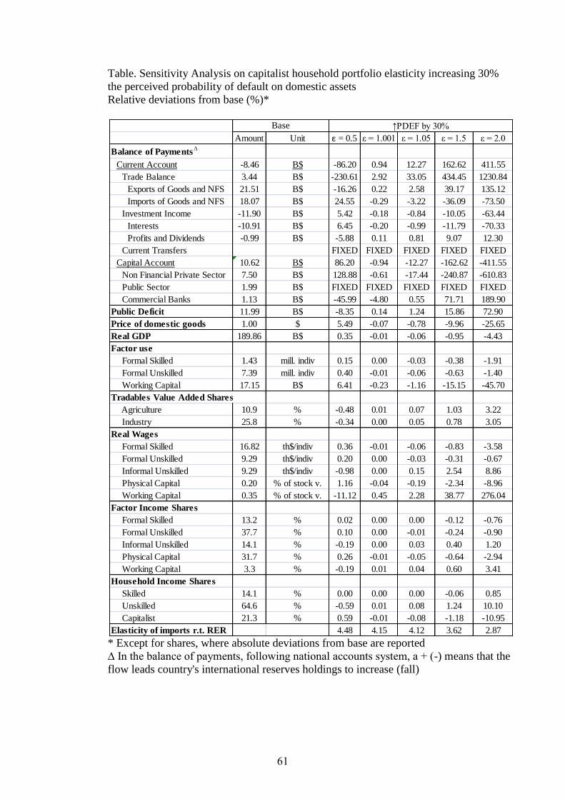
Table. Sensitivity Analysis on capitalist household portfolio elasticity increasing 30%

the perceived probability of default on domestic assets

Relative deviations from base (%)*

* Except for shares, where absolute deviations from base are reported

∆ In the balance of payments, following national accounts system, a + (-) means that the

flow leads country's international reserves holdings to increase (fall)

(Vos 1997; White 1998)

Amount Unit ε = 0.5 ε = 1.001 ε = 1.05 ε = 1.5 ε = 2.0

Balance of Payments∆

Current Account -8.46 B$ -86.20 0.94 12.27 162.62 411.55

Trade Balance 3.44 B$ -230.61 2.92 33.05 434.45 1230.84

Exports of Goods and NFS 21.51 B$ -16.26 0.22 2.58 39.17 135.12

Imports of Goods and NFS 18.07 B$ 24.55 -0.29 -3.22 -36.09 -73.50

Investment Income -11.90 B$ 5.42 -0.18 -0.84 -10.05 -63.44

Interests -10.91 B$ 6.45 -0.20 -0.99 -11.79 -70.33

Profits and Dividends -0.99 B$ -5.88 0.11 0.81 9.07 12.30

Current Transfers FIXED FIXED FIXED FIXED FIXED

Capital Account 10.62 B$ 86.20 -0.94 -12.27 -162.62 -411.55

Non Financial Private Sector 7.50 B$ 128.88 -0.61 -17.44 -240.87 -610.83

Public Sector 1.99 B$ FIXED FIXED FIXED FIXED FIXED

Commercial Banks 1.13 B$ -45.99 -4.80 0.55 71.71 189.90

Public Deficit 11.99 B$ -8.35 0.14 1.24 15.86 72.90

Price of domestic goods 1.00 $ 5.49 -0.07 -0.78 -9.96 -25.65

Real GDP 189.86 B$ 0.35 -0.01 -0.06 -0.95 -4.43

Factor use

Formal Skilled 1.43 mill. indiv 0.15 0.00 -0.03 -0.38 -1.91

Formal Unskilled 7.39 mill. indiv 0.40 -0.01 -0.06 -0.63 -1.40

Working Capital 17.15 B$ 6.41 -0.23 -1.16 -15.15 -45.70

Tradables Value Added Shares

Agriculture 10.9 % -0.48 0.01 0.07 1.03 3.22

Industry 25.8 % -0.34 0.00 0.05 0.78 3.05

Real Wages

Formal Skilled 16.82 th$/indiv 0.36 -0.01 -0.06 -0.83 -3.58

Formal Unskilled 9.29 th$/indiv 0.20 0.00 -0.03 -0.31 -0.67

Informal Unskilled 9.29 th$/indiv -0.98 0.00 0.15 2.54 8.86

Physical Capital 0.20 % of stock v. 1.16 -0.04 -0.19 -2.34 -8.96

Working Capital 0.35 % of stock v. -11.12 0.45 2.28 38.77 276.04

Factor Income Shares

Formal Skilled 13.2 % 0.02 0.00 0.00 -0.12 -0.76

Formal Unskilled 37.7 % 0.10 0.00 -0.01 -0.24 -0.90

Informal Unskilled 14.1 % -0.19 0.00 0.03 0.40 1.20

Physical Capital 31.7 % 0.26 -0.01 -0.05 -0.64 -2.94

Working Capital 3.3 % -0.19 0.01 0.04 0.60 3.41

Household Income Shares

Skilled 14.1 % 0.00 0.00 0.00 -0.06 0.85

Unskilled 64.6 % -0.59 0.01 0.08 1.24 10.10

Capitalist 21.3 % 0.59 -0.01 -0.08 -1.18 -10.95

Elasticity of imports r.t. RER 4.48 4.15 4.12 3.62 2.87

Base ↑PDEF by 30%

61

Annex VI. Bibliography

Adam, C. S. and D. L. Bevan (1998). Costs and Benefits of Incorporating Asset

Markets into CGE Models: Evidence and Design Issues. Applied Economics Discussion

Paper Series University of Oxford. No. 2002.

Agénor, P. R., A. Izquierdo, et al. (2003). The Integrated Macroeconomic Model for

Poverty Analysis. A Quantitative Macroeconomic Framework for the Analysis of

Poverty Reduction Strategies, World Bank.

Agénor, P. R., H. T. Jensen, et al. (2005). Disinflation, Fiscal Sustainability, and Labor

Market Adjustment in Turkey.

Agenor, P. R. and P. J. Montiel (1999). Development Macroeconomics, Princeton

University Press.

Blanchard, O., Ed. (2009). Macroeconomics.

Blanchflower, D. G. and A. J. Oswald (1994). The Wage Curve. London, The MIT

Press.

Bourguignon, F., B. H. Branson, et al. (1992). "Adjustment and Income Distribution: A

Micro-Macro model for counterfactual analysis." Journal of Development Economics

38(1): 23.

Bourguignon, F. and L. A. Pereira da Silva (2003). "The Impact of Economic Policies

and Income Distribution. Evaluation Techniques and Tools."

Catao, L. and E. Falcetti (2002). "Determinants of Argentina's External Trade." Journal

of Applied Economics V(1): 19-57.

Damill, M., R. Frenkel, et al. (2002). Argentina: una decada de convertibilidad. Un

analisis del crecimiento, el empleo y la distribucion del ingreso, ILO.

Dawkins, C., T. N. Srinivasan, et al. (2001). Calibration. Handbook of Econometrics. J.

J. H. E. Leamer. North-Holland, Elsevier. Chapter 58.

Decaluwe, B. and F. Nsengiyumva (1994). "Policy Impact under Credit Rationing: a

Real and Financial CGE of Rwanda." J Afr Econ 3(2): 262-308.

Dervis, K., J. de Melo, et al. (1982). General Equilibrium Models for Development

Policy. New York, Cambridge University Press for the World Bank.

Easterly, W. (1990). Portfolio Effects in a CGE Model. Devaluation in a Dollarized

Economy. Socially Relevant Policy Analysis: Structuralist Computable General

Equilibrium Models for the Developing World. L. Taylor. Cambridge MA., MIT Press.

Friedman, M. (1969). The Optimum Quantity of Money. The Optimum Quantity of

Money and Other Essays. Chicago, Aldine Publishing Company

1-50.

62

Goldberg, P. K. and N. Pavcnik (2007). "Distributional Effects of Globalization in

Developing Countries." Journal of Economic Literature 45(1): 39-82.

Harris, J. and M. Todaro (1970). "Migration, Unemployment & Development: A Two-

Sector Analysis." American Economic Review 60(1): 126-142.

Kapur, B. K. (1976). "Alternative Stabilization Policies for Less-Developed

Economies." Journal of Political Economy 84(4): 19.

Lofgren, H., R. Lee Harris, et al. (2002). A Standard Computable General Equilibrium

(CGE) Model in GAMS, IFPRI.

Mathieson, D. J. (1980). "Financial Reform and Stabilization Policy in Developing

Economy." Journal of Development Economics 7(3): 37.

Naastepad, C. W. M. (2002). "Trade-offs in stabilisation: a real-financial CGE analysis

with reference to India." Economic Modelling 19: 221-244.

Robinson, S. (1989). Multisectoral models. Handbook of Development Economics. H.

C. a. T. N. Srinivasan. Amsterdam, Elsevier Science Publishers. II.

Robinson, S. (1991). "Macroeconomics, Financial Variables, and Computable General

Equilibrium Models." World Development 19(11): 1509-1525.

Robinson, S. (2006). Macro Models and Multipliers: Leontief, Stone, Keynes, and CGE

Models. Poverty, Inequality and Development: Essays in Honor of Erik Thorbecke. A.

d. J. a. R. Kanbur. New York, Springer Science: 205-232.

Shoven, J. B. and J. Whalley (1972). "A general equilibrium calculation of the effects of

differential taxation of income from capital in the U.S." Journal of Public Economics 1:

42.

Taylor, L. (1981). IS/LM in the Tropics: Diagrammatics of the New Structuralist Macro

Critique. Economic Stabilization in Developing Countries. W. R. Cline and S.

Weintraub. Washington D.C., The Brookings Institution.

Thissen, M. (2000). Building Financial CGE Models: Data, Parameters, and the Role of

Expectations. Rijkuniversiteit Groningen, Graduate School / Research Institute Systems,

Organization and Management.

Tobin, J. (1969). "A General Equilibrium Approach To Monetary Theory." Journal of

Money, Credit and Banking 1(1): 15-29.

Tobin, J. (1981). Money and Finance in the Macro-Economic Process. Nobel Memorial

Lecture, 8 December, 1981.

Vos, R. (1997). External Finance and Adjustment Policies: A Comparative General

Equilibrium Analysis. External Finance and Adjustment: Failure and Successes in the

Developing World. K. J. a. R. Vos. London, MacMillan.

63

White, H. (1998). Aid and Macroeconomic Performance: Theory, Empirical Evidence

and Four Country Cases (International Finance and Development Series) (Hardcover)

Palgrave Macmillan

64