5/27/2016

1

Real Estate Investment

Analysis using Excel

Sing Tien Foo

Department of Real Estate

27 May 2016

Graduate Certificate in Real Estate Finance (GCREF) course

2

Website for sample template

• http://www.rst.nus.edu.sg/staff/singtienfoo/

5/27/2016

2

Mathematics of Real Estate

Finance

Quick Recap:

4

Time value of money

• The time value money is the fundamental concept of financial

mathematics

• Money changes in value over time

• Time value is created by the opportunity to invest money at some

interest rates

• Why so? Inflation, risks and productivity of capital

• “Time is money!”

– $1 today is worth more than $1 tomorrow

• “A bird in hand is better than two in the bush”

5/27/2016

3

5

Compounding Effects

• What is the value of $1 today at the end of year 2, if the interest rate

of 10% per annum?

• In a simple interest case (no compounding effects):

o FV (Year 2) = $1.0 + ($1 x 10% x 2)= $1.2

• In an annual compounding case:

o Year 1 FV1 = $1.0 x (1.1) = $1.1

o Year 2: FV2 = $1.1 x (1.1) = $1.21

o FV(year 2) = PV x (1+i) x (1+i) = PV (1+i)2 = $1 x (1.1)2 = $1.21

• Difference = $1.21– $1.20 = $0.01 is the COMPOUNDING effects!

• In a half yearly compounding case:

o FV(year 2) = PV x [(1+i/2) x (1+i/2) x (1+i/2) x (1+i/2)] = PV x (1 +i/2)nx2

o FV(year 2) = $1 x (1 + 0.1/2)4 = $1.2155

6

Simple interest versus compound interest

0

20000

40000

60000

80000

100000

120000

140000

160000

180000

200000

1 2 3 4 5 6 7 8 9 10 11 12 13 14 15 16 17 18 19 20 21 22 23 24 25 26 27 28 29 30

Simple interest rate

Compounding interest rate

Year

5/27/2016

4

7

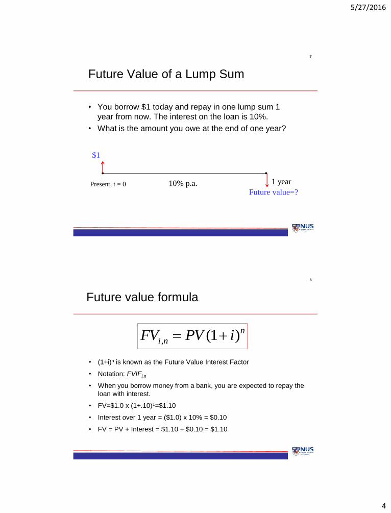
Future Value of a Lump Sum

• You borrow $1 today and repay in one lump sum 1

year from now. The interest on the loan is 10%.

• What is the amount you owe at the end of one year?

Present, t = 0 1 year

$1

Future value=?10% p.a.

8

Future value formula

• (1+i)n is known as the Future Value Interest Factor

• Notation: FVIFi,n

• When you borrow money from a bank, you are expected to repay the

loan with interest.

• FV=$1.0 x (1+.10)1=$1.10

• Interest over 1 year = ($1.0) x 10% = $0.10

• FV = PV + Interest = $1.10 + $0.10 = $1.10

n

ni iPVFV )1(,

5/27/2016

5

9

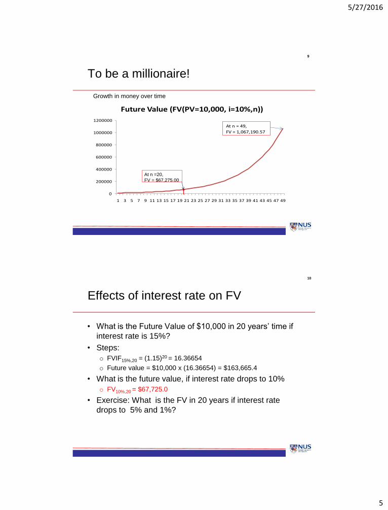
To be a millionaire!

0

200000

400000

600000

800000

1000000

1200000

1 3 5 7 9 11 13 15 17 19 21 23 25 27 29 31 33 35 37 39 41 43 45 47 49

Future Value (FV(PV=10,000, i=10%,n))

At n = 49,

FV = 1,067,190.57

At n =20,

FV = $67,275.00

Growth in money over time

10

Effects of interest rate on FV

• What is the Future Value of $10,000 in 20 years’ time if

interest rate is 15%?

• Steps:

o FVIF15%,20 = (1.15)20 = 16.36654

o Future value = $10,000 x (16.36654) = $163,665.4

• What is the future value, if interest rate drops to 10%

o FV10%,20 = $67,725.0

• Exercise: What is the FV in 20 years if interest rate

drops to 5% and 1%?

– FV 5%,20 = $10,000 x (1.05)20 = $26.532.98

– FV 1%,20 = $10,000 x (1.01)20 = $12,201.90

5/27/2016

6

11

Interest rate sensitivity

$0

$100,000

$200,000

$300,000

$400,000

$500,000

$600,000

$700,000

$800,000

$900,000

$1,000,000

1 6 11 16 21 26 31 36 41 46 51 56 61 66 71 76 81 86 91

FV

($10,0

00,

i, n

)

Year

5% 10% 15% 20%

>25 >32 >48 >94

12

Interest rate sensitivity

0

50000

100000

150000

200000

250000

300000

350000

400000

1%

2%

3%

4%

5%

6%

7%

8%

9%

10

%

11

%

12

%

13

%

14

%

15

%

16

%

17

%

18

%

19

%

20

%

What is the Future Value of $10,000 in 20-year time at i % interest rate?

i = 20%: $383,376

i =15%: $163,665

i=1%: $12,202

5/27/2016

7

13

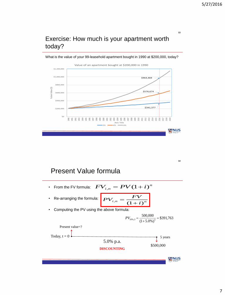
Exercise: How much is your apartment worth

today?

What is the value of your 99-leasehold apartment bought in 1990 at $200,000, today?

$0

$200,000

$400,000

$600,000

$800,000

$1,000,000

$1,200,00019

90

1991

1992

1993

1994

1995

1996

1997

1998

1999

2000

2001

2002

2003

2004

2005

2006

2007

2008

2009

2010

2011

2012

2013

2014

2015

2016

2017

2018

2019

Futu

re V

alue

($)

Axis Title

Value of an apartment bought at $200,000 in 1990

2% 4% 6%

$964,469

$341,377

$576,674

14

Present Value formula

• From the FV formula:

• Re-arranging the formula:

• Computing the PV using the above formula:

n

ni iPVFV )1(,

nnii

FVPV

)1(,

763,391$%)0.51(

000,50053%,10

PV

Today, t = 0 5 years

Present value=?

$500,0005.0% p.a.

DISCOUNTING

5/27/2016

8

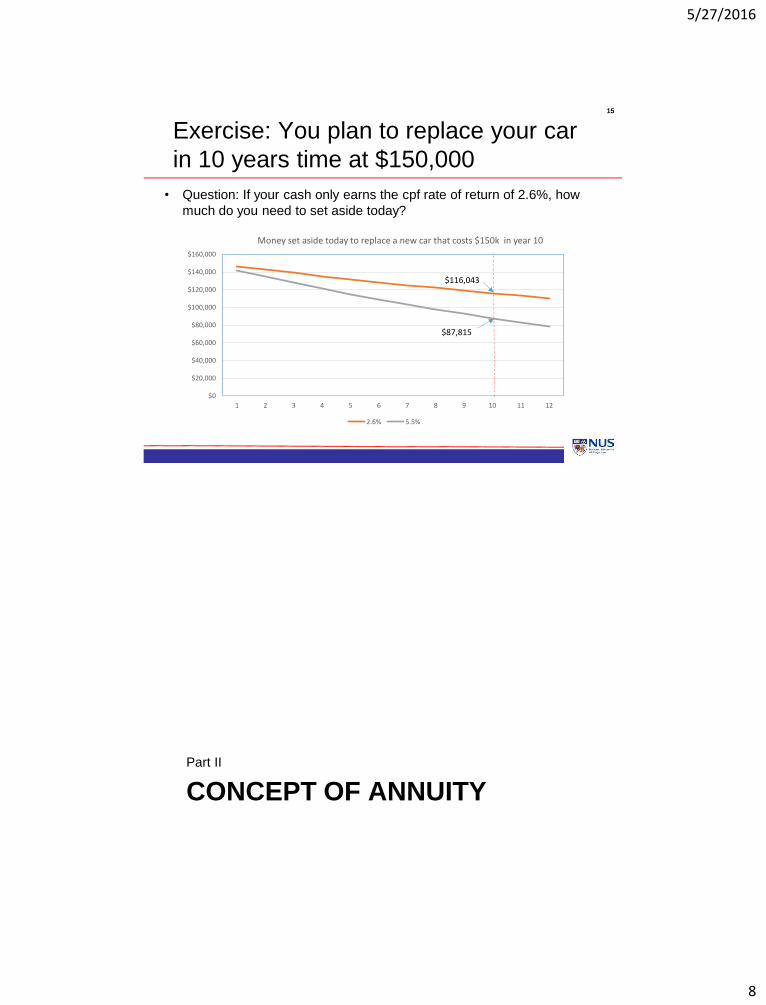
15

Exercise: You plan to replace your car

in 10 years time at $150,000

• Question: If your cash only earns the cpf rate of return of 2.6%, how

much do you need to set aside today?

$0

$20,000

$40,000

$60,000

$80,000

$100,000

$120,000

$140,000

$160,000

1 2 3 4 5 6 7 8 9 10 11 12

Money set aside today to replace a new car that costs $150k in year 10

2.6% 5.5%

$116,043

$87,815

CONCEPT OF ANNUITY

Part II

5/27/2016

9

18

Concept of Annuity

• Instead of a single lump sum payment, we receive a

series of payments made at equal intervals

• The series of payments is known as “Annuities”

• There are two types of annuity

o Annuity Due = payment at the beginning of period

o Regular Annuity= payment at the end of period

• Mortgage payments are usually made at the end of month

• Rental payments are made at the beginning of the month

20

Present Value of Annuity (PFA)

• Suppose you can pay $10,000 for 3 years for a loan

which you take now. What is the loan amount if interest

rate=10% compounded annually?

• $10,000 [(1+0.1)-1 + (1+0.1)-2+ (1+0.1)-3] = $24,868.52

Sing Tien Foo, Dept of Real

Estate, NUS

$10,000$10,000 $10,000

now 1 year 2 years 3 years

Present value?

Year 1 $10,000 * (1 + 0.1)-1 $9,090.909

Year 2 $10,000 * (1+ 0.1) -2 $8,264.463

Year 3 $10,000 * (1+ 0.1)-3 $7,513.148

sum $24,868.52

5/27/2016

10

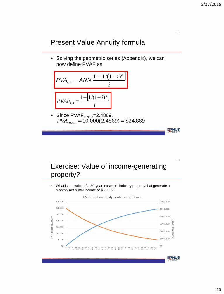
21

Present Value Annuity formula

• Solving the geometric series (Appendix), we can

now define PVAF as

• Since PVAF10%,3=2.4869,

i

iPVAF

n

ni

)1/(11,

869,24$)4869.2(000,103%,10 PVA

i

iANNPVA

n

ni

)1/(11,

22

Exercise: Value of income-generating

property?

• What is the value of a 30-year leasehold industry property that generate a

monthly net rental income of $3,000?

$0

$100,000

$200,000

$300,000

$400,000

$500,000

$600,000

$0

$500

$1,000

$1,500

$2,000

$2,500

$3,000

$3,500

1 14 27 40 53 66 79 92 105

118

131

144

157

170

183

196

209

222

235

248

261

274

287

300

313

326

339

352

Cum

ulat

ive

Rent

al ($

)

PV o

f net

rent

al A

nnui

ty

PV of net monthly rental cash flows

5/27/2016

11

23

Lecture Outline

• Investing in real estate

• Cash flow pro-forma

• Investment rule – decision criteria

• Case study

• Real Estate Investment Risks

• Summary

• http://www.rst.nus.edu.sg/staff/singtienfoo/

24

Real Estate Investment Analysis

• Motivations for property purchase• Owner occupation versus investment• Reasons for owner occupation:– Pride of ownership– A form of wealth– Consumption of housing services w/o rent

• Perspectives change when purchase is for investment purposes:

– Generate net income

– Capital gains

– Diversification

– Preferential tax benefits

5/27/2016

12

26

Operating Cash Flows

Property level unlevered cash flows

Gross Rent or Potential Gross Income

Effective Gross Income

Operating Expenses

Net Operating Income or NOI

Capital Expenditure

Leverage Effects

Debt Service

27

Property level cash flow pro-forma

(unleveraged)

• Operating cash flows (all years):Potential Gross Income = PGI

Less Vacancy Allowance = - v

+ Other Income (eg, parking, laundry) = +OI

Effective Gross Income = EGI

- Operating Expenses = - OE

Net Operating Income = NOI

• Reversion cash flow (disposal of asset):Property Value at time of sale = V

- Selling Expenses (eg, brokerage fees, legal fees) = - SE

Property-level Before-tax Cash Flow = PBTCF

(Net sale value)

5/27/2016

13

28

Potential Gross Income (PGI)

• Rental income assuming 100% occupancy

• Important issue: Contract rent or market rent?– Market rent is the most probable rent a property will

command, if placed for lease on the open market

– Contract rent is actual rent paid under the contractual agreement between landlord and tenants

• If a property is subject to long-term leases, contract rent will be used– eg. sale-leaseback leases in some industrial properties

29

Types of Leases

• Straight lease

– “Level” lease payments

• Step-up or graduated lease

– Rent increases on a predetermined schedule

• Indexed lease

– Rent tied to an inflation index, such as Consumer

Price Index, Union wage index, etc.

• Percentage lease

– Rent includes percentage of tenant’s sales

5/27/2016

14

30

Effective Gross Income

• Vacancy and collection loss – Historical experience

– Competing properties in the market

– “Natural vacancy” rate• Vacancy rate that is expected in a stable or equilibrium

market

• Miscellaneous income– Car-parking collection

– Signage and advertising space

– vending machines

– Rentals for clubhouse / promotional space

31

Operating Expenses

• Ordinary and regular expenditures necessary to

keep a property functioning competitively

• Fixed expenses that do not vary with occupancy:

– insurance,

– property taxes

• Variable expenses that vary with occupancy:

– utilities

– maintenance and supplies

– service contracts

5/27/2016

15

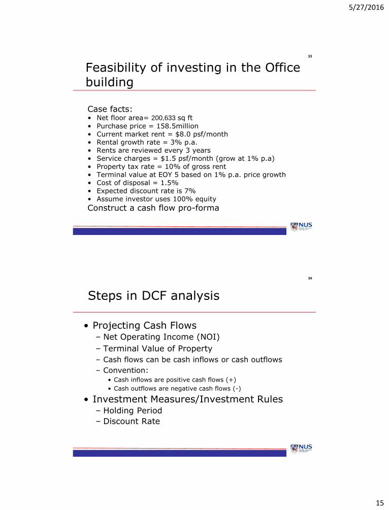
33

Feasibility of investing in the Office building

Case facts:• Net floor area= 200,633 sq ft

• Purchase price = 158.5million• Current market rent = $8.0 psf/month• Rental growth rate = 3% p.a.• Rents are reviewed every 3 years• Service charges = $1.5 psf/month (grow at 1% p.a)• Property tax rate = 10% of gross rent• Terminal value at EOY 5 based on 1% p.a. price growth• Cost of disposal = 1.5%• Expected discount rate is 7%• Assume investor uses 100% equity

Construct a cash flow pro-forma

34

Steps in DCF analysis

• Projecting Cash Flows– Net Operating Income (NOI)

– Terminal Value of Property

– Cash flows can be cash inflows or cash outflows

– Convention: • Cash inflows are positive cash flows (+)

• Cash outflows are negative cash flows (-)

• Investment Measures/Investment Rules– Holding Period

– Discount Rate

5/27/2016

16

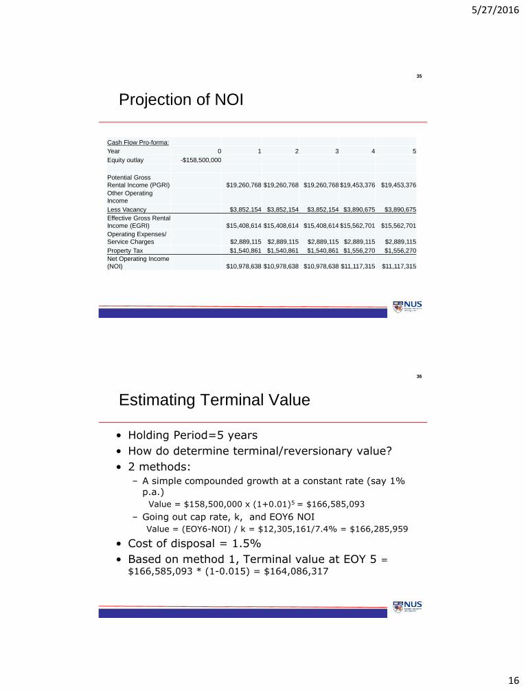
35

Projection of NOI

Cash Flow Pro-forma:

Year 0 1 2 3 4 5

Equity outlay -$158,500,000

Potential Gross

Rental Income (PGRI) $19,260,768 $19,260,768 $19,260,768 $19,453,376 $19,453,376

Other Operating

Income

Less Vacancy $3,852,154 $3,852,154 $3,852,154 $3,890,675 $3,890,675

Effective Gross Rental

Income (EGRI) $15,408,614 $15,408,614 $15,408,614 $15,562,701 $15,562,701

Operating Expenses/

Service Charges $2,889,115 $2,889,115 $2,889,115 $2,889,115 $2,889,115

Property Tax $1,540,861 $1,540,861 $1,540,861 $1,556,270 $1,556,270

Net Operating Income

(NOI) $10,978,638 $10,978,638 $10,978,638 $11,117,315 $11,117,315

36

Estimating Terminal Value

• Holding Period=5 years

• How do determine terminal/reversionary value?

• 2 methods:

– A simple compounded growth at a constant rate (say 1% p.a.)

Value = $158,500,000 x (1+0.01)5 = $166,585,093

– Going out cap rate, k, and EOY6 NOI

Value = (EOY6-NOI) / k = $12,305,161/7.4% = $166,285,959

• Cost of disposal = 1.5%

• Based on method 1, Terminal value at EOY 5 =

$166,585,093 * (1-0.015) = $164,086,317

5/27/2016

17

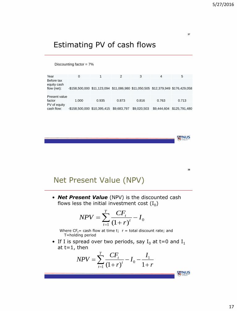
37

Estimating PV of cash flows

Year 0 1 2 3 4 5

Before tax

equity cash

flow (net): -$158,500,000 $11,123,094 $11,086,980 $11,050,505 $12,379,949 $176,429,058

Present value

factor 1.000 0.935 0.873 0.816 0.763 0.713

PV of equity

cash flow: -$158,500,000 $10,395,415 $9,683,797 $9,020,503 $9,444,604 $125,791,480

Discounting factor = 7%

38

Net Present Value (NPV)

• Net Present Value (NPV) is the discounted cash flows less the initial investment cost (I0)

Where CFt= cash flow at time t; r = total discount rate; and T=holding period

• If I is spread over two periods, say I0 at t=0 and I1

at t=1, then

r

II

r

CFNPV

T

tt

t

1)1(

10

1

0

1 )1(I

r

CFNPV

T

tt

t

5/27/2016

18

39

Profitability Index

• Profitability Index (PI) is the ratio of the present value of cash inflows to the initial equity invested (present value of cash outflows).

• PI = PV(inflows)/PV(outflows)

• PI greater than 1 implies that expected return exceeds the discount rate.

40

Internal Rate of Return (IRR)

• The Internal Rate of Return (IRR) is the rate of return required to make the present values of future cash flows equal to the cost of the investment.

T=holding period

T

tt

t

IRR

CFI

1 )1(

5/27/2016

19

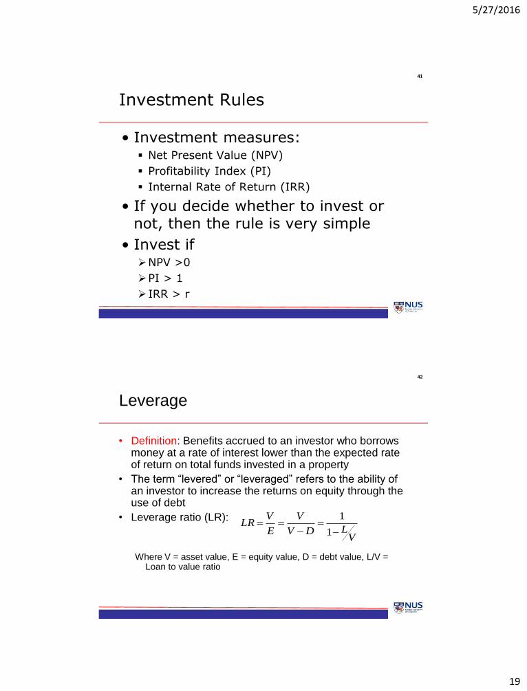
41

Investment Rules

• Investment measures: Net Present Value (NPV)

Profitability Index (PI)

Internal Rate of Return (IRR)

• If you decide whether to invest or not, then the rule is very simple

• Invest ifNPV >0

PI > 1

IRR > r

42

Leverage

• Definition: Benefits accrued to an investor who borrows money at a rate of interest lower than the expected rate of return on total funds invested in a property

• The term “levered” or “leveraged” refers to the ability of an investor to increase the returns on equity through the use of debt

• Leverage ratio (LR):

Where V = asset value, E = equity value, D = debt value, L/V = Loan to value ratio

VLDV

V

E

VLR

1

1

5/27/2016

20

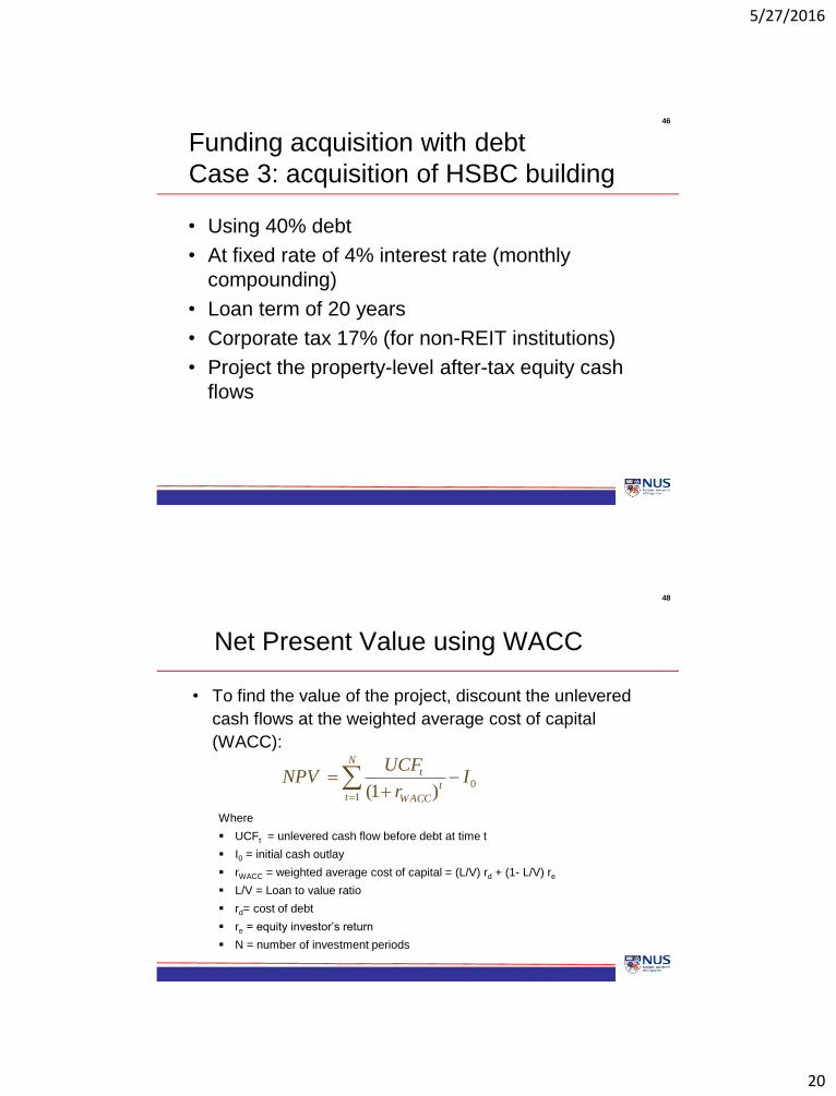
46

Funding acquisition with debt

Case 3: acquisition of HSBC building

• Using 40% debt

• At fixed rate of 4% interest rate (monthly

compounding)

• Loan term of 20 years

• Corporate tax 17% (for non-REIT institutions)

• Project the property-level after-tax equity cash

flows

48

Net Present Value using WACC

• To find the value of the project, discount the unlevered

cash flows at the weighted average cost of capital

(WACC):

Where

UCFt = unlevered cash flow before debt at time t

I0 = initial cash outlay

rWACC = weighted average cost of capital = (L/V) rd + (1- L/V) re

L/V = Loan to value ratio

rd= cost of debt

re = equity investor’s return

N = number of investment periods

N

tt

WACC

t Ir

UCFNPV

1

0)1(

5/27/2016

21

49

Determining WACC

• WACC formula is dependent on the capital structure at

the firm level, not at the project level

• Let re = levered equity return; rd =c ost of debt; =

corporate tax rate;

• Total Capital V = E (equity) + D (Debt)

• For a firm with a capital structure of D/V = 0.4 E/V = 0.6,

and re = 10% and rd = 4% and = 17%

edWACC rDE

Er

DE

Dr

)1(

%328.7%106.0%)171(%44.0 WACCr

51

Capital Expenditures (CAPEX)

• Expenditures that materially increase value of a structure or prolong its life:– Roof replacement

– Additions and alterations

– HVAC Replacement

– Resurfacing of parking areas

– Tenant improvements

• Estimating CAPEX:

– Sinking fund: An amount invested annually that compounds to the needed CAPEX in a future year.

– Straight-line: For an expenditure n years away, an amount equal to the needed CAPEX divided by n.

– Actual expenditures: The actual amount expected in each year of the expected holding period

5/27/2016

22

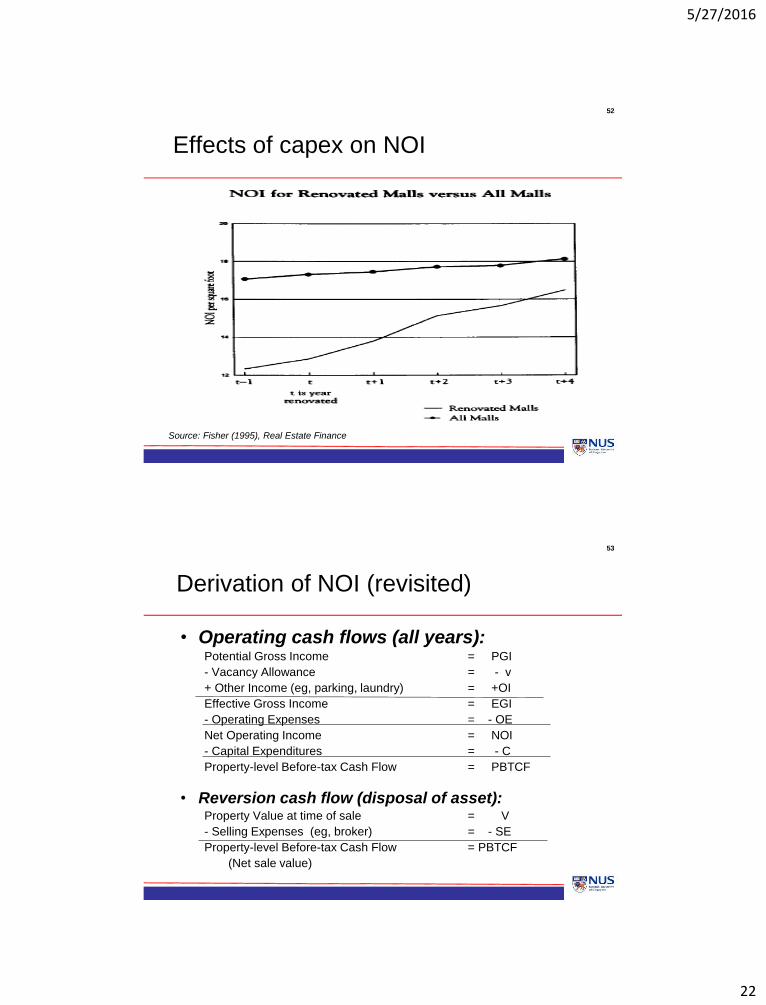
52

Effects of capex on NOI

Source: Fisher (1995), Real Estate Finance

53

Derivation of NOI (revisited)

• Operating cash flows (all years):Potential Gross Income = PGI

- Vacancy Allowance = - v

+ Other Income (eg, parking, laundry) = +OI

Effective Gross Income = EGI

- Operating Expenses = - OE

Net Operating Income = NOI

- Capital Expenditures = - C

Property-level Before-tax Cash Flow = PBTCF

• Reversion cash flow (disposal of asset):Property Value at time of sale = V

- Selling Expenses (eg, broker) = - SE

Property-level Before-tax Cash Flow = PBTCF

(Net sale value)

5/27/2016

23

54

Net Operating Income (NOI) and

Capital Expenditure (Capex)

• Capex

– Reserve for replacements

– Tenant improvement

– Leasing commissions

• Above-line or below-line approach

Above Line:

EGI

- OE

- CAPX

= NOI

Below Line:

EGI

- OE

= NOI

- CAPX

= Net Cash Flow

55

Asset Enhancement Initiatives (AEI)

Case 2: The Extension of IMM Building

• CAPITAMALL Trust (CMT) acquired the IMM Building in Jurong for $264.5 million in 2003

• IMM completed a major revamp in Dec 2007 by building a three-storey annexed block on the ground level open-air carpark

• The first floor of the new block will consist of retail space while the parking space will be moved to the upper floors.

• CMT expects IMM purchase to raise returns.

• By Vladimir Guevarra.

• 14 May 2003

• Straits Times

5/27/2016

24

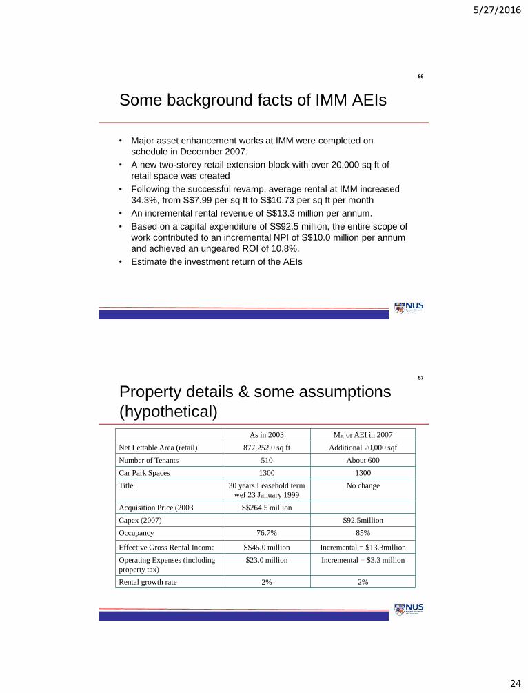
56

Some background facts of IMM AEIs

• Major asset enhancement works at IMM were completed on

schedule in December 2007.

• A new two-storey retail extension block with over 20,000 sq ft of

retail space was created

• Following the successful revamp, average rental at IMM increased

34.3%, from S$7.99 per sq ft to S$10.73 per sq ft per month

• An incremental rental revenue of S$13.3 million per annum.

• Based on a capital expenditure of S$92.5 million, the entire scope of

work contributed to an incremental NPI of S$10.0 million per annum

and achieved an ungeared ROI of 10.8%.

• Estimate the investment return of the AEIs

57

Property details & some assumptions

(hypothetical)

As in 2003 Major AEI in 2007

Net Lettable Area (retail) 877,252.0 sq ft Additional 20,000 sqf

Number of Tenants 510 About 600

Car Park Spaces 1300 1300

Title 30 years Leasehold term

wef 23 January 1999

No change

Acquisition Price (2003 S$264.5 million

Capex (2007) $92.5million

Occupancy 76.7% 85%

Effective Gross Rental Income S$45.0 million Incremental = $13.3million

Operating Expenses (including

property tax)

$23.0 million Incremental = $3.3 million

Rental growth rate 2% 2%

5/27/2016

25

58

Avoiding Pitfalls in DCF applications

• “GIGO” – Garbage in garbage out

• Common mistakes

– Rental / income growth assumption is too high

– Capital improvement and going-out cap rate projections are too low

– Discount rate is too high

• Errors are hidden in the DCF model, which may create false expectation for investors in the long-run

• Consequences of the mistakes

– Unrealistic expectations

– Long-run undermining credibility of DCF methodology

· Read the “fine print”.

· Look for “hidden assumptions”.

· Check realism of assumptions.

Thank you

59

References

• Ling, D.C. and Archer, W.R. (2005), Real Estate

Principles: A Value Approach, McGraw Hill

• Brueggeman, W.B. and Fisher, J.D. (2011), Real

Estate Finance and Investments, 14th Edition,

McGraw Hill