Re-evaluating the Effectiveness of Inflation Targeting
50
Electronic copy available at: https://ssrn.com/abstract=3238084 Re-evaluating the Effectiveness of Inflation Targeting Omid M. Ardakani † N. Kundan Kishor ‡ Suyong Song § Abstract This paper estimates the treatment effect of inflation targeting on macroeconomic variables using a semiparametric single index method by taking into account the model misspecification of parametric propensity scores. Our study uses a broader set of preconditions for inflation targeting and macroeconomic outcome variables than the existing literature. The results suggest no significant difference in the inflation level and inflation volatility between targeters and non-targeters after the adoption of inflation targeting. We find that inflation targeting reduces sacrifice ratio and interest rate volatility in the developed economies, and that it enhances fiscal discipline in both the industrial and developing countries. Keywords: Inflation Targeting, Propensity Score, Treatment Effects, Single Index Model. JEL Classification: C14, E4, E5. † Department of Economics, Georgia Southern University, Savannah, GA 31419 ([email protected]) ‡ Department of Economics, University of Wisconsin-Milwaukee, Milwaukee, WI 53211 ([email protected]) § Department of Economics, University of Iowa, Iowa City, IA 52242 ([email protected]) 1
Transcript of Re-evaluating the Effectiveness of Inflation Targeting

Electronic copy available at: https://ssrn.com/abstract=3238084
Re-evaluating the Effectiveness of Inflation Targeting
Omid M. Ardakani † N. Kundan Kishor ‡ Suyong Song §
Abstract
This paper estimates the treatment effect of inflation targeting on macroeconomicvariables using a semiparametric single index method by taking into account the modelmisspecification of parametric propensity scores. Our study uses a broader set ofpreconditions for inflation targeting and macroeconomic outcome variables than the existingliterature. The results suggest no significant difference in the inflation level and inflationvolatility between targeters and non-targeters after the adoption of inflation targeting.We find that inflation targeting reduces sacrifice ratio and interest rate volatility in thedeveloped economies, and that it enhances fiscal discipline in both the industrial anddeveloping countries.
Keywords: Inflation Targeting, Propensity Score, Treatment Effects, Single Index Model.JEL Classification: C14, E4, E5.
†Department of Economics, Georgia Southern University, Savannah, GA 31419([email protected])
‡Department of Economics, University of Wisconsin-Milwaukee, Milwaukee, WI 53211 ([email protected])§Department of Economics, University of Iowa, Iowa City, IA 52242 ([email protected])
1

Electronic copy available at: https://ssrn.com/abstract=3238084
1 Introduction
Explicit inflation targeting (IT) has been increasingly adopted as a monetary policy strategy
to curb actual inflation over the medium-to-long horizon. Under the IT regime, a central bank
publicly announces a target inflation rate and then uses different monetary policy tools to bridge
the gap between actual inflation and the target. One of the impressive features of this monetary
policy strategy is no country has given up this regime after its adoption. The Reserve Bank of
New Zealand became the first central bank to adopt the IT regime in 1990. The increasing
popularity of the IT regime has spawned a great deal of academic interest in its effectiveness.
Even though the amount of work on the effectiveness of IT has increased manifold in the last
two decades, there is no consensus on the overall impact of this regime on the macroeconomy.
One view suggests a significant effect of IT on macroeconomic performance; the opposite
suggests that the impact of the IT regime has been mostly insignificant. Several researchers find
inflation targeting is successful in reducing inflation and inflation variability (Neumann and von
Hagen (2002), Wu (2004), Vega and Winkelried (2005), Mishkin and Schmidt-Hebbel (2007),
and Creel and Hubert (2010)). Among them, Mishkin and Schmidt-Hebbel (2001) argue the IT
regime not only causes a reduction in inflation and inflation variability, but lessens the sacrifice
ratio, output volatility, and inflation expectations. In a recent paper Eo and Lie (2017) show that
combined with the standard Taylor rule, the optimal medium-run inflation target significantly
reduces fluctuations in inflation originating from the cost-push shocks and results in a similar
level of welfare to that associated with the Ramsey optimal policy. The literature also postulates
indirect benefits from inflation targeting in terms of reduction in exchange rate volatility (Rose
(2007) and Lin (2010)),1 interest rates (Filho (2011)), fiscal indiscipline (Minea and Tapsoba
(2014) and Lucotte (2012)), and actual dollarization (Lin and Ye (2013)). However, Johnson
(2002) and Angeriz and Arestis (2007) find the IT regime does not reduce the variability of
expected inflation. Similar viewpoints have been expressed by Ball and Sheridan (2003), who
1Lin (2010) finds inflation targeting lowers real and nominal exchange rate volatility only in industrialeconomies, but increases them in developing countries.
2

Electronic copy available at: https://ssrn.com/abstract=3238084
argue there is no evidence that IT reduces inflation variability, output volatility, and output
growth. Lin and Ye (2007) also find IT has no significant effects on either inflation or inflation
variability. They suggest both targeters and non-targeters have experienced an unexpected
reduction in inflation.
Our study contributes to the existing IT impact literature in several ways. Our econometric
approach improves on the treatment effect literature that has been used to estimate the impact
of IT. The parameter of interest is the average treatment effect on the treated which is defined
as the difference in mean outcomes by the IT status for the countries that actually have adopted
the IT framework. A few methods have been proposed to take into account the self-selection
problem that may arise because a central bank’s decision to explicitly target inflation is related
to the benefits from the adoption of IT. This leads to a biased causal effect. Previous studies (e.g.
Lin and Ye (2013) and de Mendonca and de Guimaraes (2012)) have attempted to overcome the
selection bias problem by parametrically estimating propensity scores and matching treated and
control units to mimic a randomized experiment. The parametric approach to estimating the
average treatment effect of inflation targeting suffers from model misspecification and provides
inconsistent estimates of the propensity scores, when the true data generating process is very
different from that based on a pre-specified functional form of the model. The nonparametric
approach proposed by Hirano, Imbens and Ridder (2003) could be a possible solution to the
issue. The approach, however, suffers from the “curse of dimensionality,” which refers to the
problem where the high dimension of the variable space due to large number of covariates
in their logit series estimation makes the performance of the nonparametric estimator worse.
To take into account these econometric problems, we adopt the semiparametric single index
method suggested by Klein and Spady (1993), which mitigates the issue of high dimensionality,
while the functional form of the propensity score and the distribution of the error term are
still unknown. Following Dehejia and Wahba (1999, 2002), we first show that the average
treatment effect on the treated can be identified under two conditions: (1) IT is independent
of the outcomes given the covariates used for the propensity scores estimates, (2) propensity
3

Electronic copy available at: https://ssrn.com/abstract=3238084
scores are assumed to be less than one. Second, we explain the estimation in two steps: in the
first step, we estimate propensity scores using the single index estimator, and in the second step,
we estimate the average treatment effect on the treated using the propensity score matching
estimator. In fact, Song (2014) shows that the average treatment effect can be identified by the
semiparametric two-step approach and the estimator is consistent and asymptotically normally
distributed under regularity conditions.
Most of the research on the treatment effect of inflation targeting has examined its impact
on the level of inflation and inflation volatility. One of the proposed benefits of having a
monetary policy regime with a nominal anchor is it enhances the credibility of central banks. As
a consequence, the volatility of important macroeconomic variables such as the exchange rate
and interest rate may be affected in addition to its impact on the sacrifice ratio. The adoption
of IT may also nudge the fiscal policymakers to adopt fiscally responsible policies. Moreover,
inflation targeting may also bring inflation down at a lower cost, in terms of lower sacrifice
ratio. The second contribution of our paper is to examine the effectiveness of the IT regime by
not only investigating its impact on inflation and inflation volatility, but also macroeconomic
variables such as the level of government debt, the sacrifice ratio, interest rate volatility, and
exchange rate volatility.
The propensity score analysis for the IT regime involves estimating the probability of
conducting IT in the first stage. The existing studies that have adopted the treatment effect
approach have ignored the role of financial market development in the probability of adopting
inflation targeting. This is in contrast to the literature on the IT precondition literature where
researchers have strongly opined that financial market development is one of the most important
criteria for the adoption and success of the IT regime (Amato and Gerlach (2002) and Bernanke
and Woodford (2005)). Our third contribution is that, in addition to the macroeconomic
predictors used in the previous studies, we use the central bank assets-GDP ratio and the private
credit-GDP ratio as proxies for financial market development in the first stage to estimate the
probability of adopting IT.
4

Electronic copy available at: https://ssrn.com/abstract=3238084
We find several interesting results from the semiparametric index models. First, we find that
there is no significant difference in the impact on inflation and inflation volatility in inflation
targeter versus non-inflation targeters in both the developed and developing economies. In
contrast, the parametric propensity scores suggest a significant decline in inflation volatility in
the developing countries. Secondly, the adoption of IT leads to significant decline in the sacrifice
ratio and volatility of the interest rate in the developed inflation targeters, providing evidence on
the credibility hypothesis. However, we do not find a significant impact of IT on the sacrifice ratio
and interest rate volatility in the developing economies. The adoption of IT leads to an increase
in volatility of exchange rates in the developed economies, whereas it reduces the exchange rate
volatility in developing economies. Our results show that adoption of IT leads to improvement
in debt-GDP ratio in both the developed and the developing economies. Overall, our results
suggest that IT as a monetary policy strategy seems to have benefited developed economies more
than developing economies mainly through the credibility enhancement channel. However, the
estimated treatment effect of IT using parametric propensity score suggests that the developing
countries have benefited disproportionately in terms of higher reduction in inflation, the
exchange rate and interest rate volatility after the adoption of IT as a monetary policy regime.
The discrepancy among treatment effect estimates from parametric and semiparametric models
suggests the possibility of model misspecification in the parametric propensity scores. As a
sensitivity analysis, we use conventional covariates, contemporaneous covariates, and a smaller
sample period (before the 2008 financial crisis). The estimation results confirm that our
approach is robust to various scenarios and the approach to estimating propensity scores in the
first stage has significant impacts on the treatment effects.
The remainder of this paper is organized in the following order. Section 2 reviews the IT
effectiveness from theoretical and practical points of view. Section 3 describes the data set.
Section 4 examines and compares the impact of IT using single index, nonparametric, and
parametric propensity scores and explains the problems associated with the latter two models.
Section 5 checks whether the results are robust to the inclusion of different sets of covariates
5

Electronic copy available at: https://ssrn.com/abstract=3238084
and the use of the pre-crisis sample period. Section 6 gives some concluding remarks.
2 Background
2.1 Theoretical Context
Since the adoption of explicit inflation targeting by the Reserve Bank of New Zealand in
1990, there has been an explosion of interest in the theoretical and empirical work on the effect
of inflation targeting. Most of the theoretical work has focused on examining whether inflation
targeting is an optimal monetary policy strategy. Central banks adopt explicit inflation targeting
by setting an instrument such that the inflation forecast and inflation target become identical.
Svensson (1996) interprets inflation targeting as a targeting rule that specifies a target variable
and target level to minimize a loss function. The inflation forecast targeting loss function can
be written as
L(πt+τ|t) =12
�
(πt+τ|t −π∗)2 +λy2t+τ|t
�
, (1)
where πt+τ|t is the τ-step ahead forecast of the inflation rate as a function of the interest rate,
it , conditional upon information available in year t. π∗ denotes the inflation target level. λ≥ 0
is the relative weight on output stabilization and yt+τ|t is the τ-step ahead forecast of output.
Central banks’ objective in period t is to choose a sequence of interest rates, {it}∞t=τ, to minimize
the expected sum of discounted loss
minit
E∞∑
t=τ
δτ−t L(πt+τ|t), (2)
where E is expectations conditional on information in year t and δ is the discount factor. The
first-order condition for minimizing Equation (2) can be written as
6

Electronic copy available at: https://ssrn.com/abstract=3238084
∂E∞∑
τ=tδτ−t L(πt+τ|t)
∂ it= E
�
δτ−t(πt+τ|t(it)−π∗)∂ πt+τ|t
∂ it
�
= 0. (3)
Consequently, it follows
πt+τ|t = π∗. (4)
In an explicit inflation targeting regime, the central bank commits to minimizing a loss
function, such that the target would be equal to the τ-step ahead forecast.2 The effectiveness
of this monetary policy framework can be considered through the two channels of aggregate
demand and expectations. In the aggregate demand channel, monetary policy affects aggregate
demand and then inflation via the Phillips curve. In the expectations channel, monetary
policy affects inflation by anchoring inflation expectations. The latter view suggests the
inflation forecast as a target provides better information about central bank actions and
therefore influences expectations. This transparency increases the effectiveness of monetary
policy (Svensson (1999)). As in Woodford (2005) and Svensson (2005a), a higher degree of
transparency improves the conduct of monetary policy. The consequences of the transparency
of central banks are a reduction in uncertainty about future policy actions and anchoring actual
inflation and inflation volatility.
In a theoretical framework, Demertzis and Hallett (2007) show the transparency of central
banks has no effect on the level of inflation and output, but decreases the volatility of inflation
and the output gap. Morris and Shin (2002) address this issue through the lens of welfare
effects. They argue greater transparency does not necessarily improve social welfare. In an
economy with highly volatile inflation, the central bank is unlikely to have more information
2Please refer to Svensson (1996) for details.
7

Electronic copy available at: https://ssrn.com/abstract=3238084
than the private sector, and private information may crowd out the central bank’s disclosed
information, which leads to a greater volatility. However, Svensson (2005b) argues the results
of Morris and Shin (2002) are misinterpreted as an “anti-transparency.” He shows that the
higher degree of transparency increases the social welfare. Recently there has been a surge of
interest in the theoretical framework of inflation targeting effectiveness through the channels
of expectations, transparency, and the accountability of central banks.The consensus from the
theoretical literature is that focusing the impact of IT on level of inflation and inflation volatility
is not sufficient to measure the effectiveness of IT on macroeconomy. Therefore, this study
attempts to examine the impact of IT on not only the conventional macroeconomic outcomes,
but also the variables that may be affected due to expectations, credibility and transparency
channels.
2.2 Empirical Background
The existing empirical literature on the effectiveness of inflation targeting suffers from three
problems. The first issue is the estimation methodology. Second, the variables used to find the
likelihood of adopting inflation targeting ignore the conventional wisdom and extant literature
suggesting the role of preconditions in the effectiveness of inflation targeting. Third, most of the
work on inflation targeting using the treatment effect methodology has estimated the impact of
this regime on the level of inflation and inflation volatility. The literature lacks a comprehensive
study on a variety of outcome variables.
The empirical research on the effectiveness of inflation targeting has primarily attempted to
examine its impact on the level of inflation and inflation volatility. Initially most of the work
focused on examining the effectiveness of the IT regime by performing some form of an event
study analysis. This strand of literature compared the behavior of inflation and its volatility
before and after the adoption of the IT regime. The event study approach was criticized on
the grounds that this methodology does not take into account the changes in the behavior of
inflation that would have taken place anyway in the absence of the IT regime. The criticism
8
Electronic copy available at: https://ssrn.com/abstract=3238084
was based on the global fall in inflation and inflation volatility that took place during the time
this regime was in place in different countries.
With reference to the estimation methodology, Ball and Sheridan (2003) find the effect
of IT by comparing improvements in targeters to improvements in non-targeters. They
apply the difference-in-differences approach. To reduce the bias from the correlation of the
outcome before the adoption of IT and the targeting dummy, they add the initial value of
the outcome to the differences regression. Ball and Sheridan (2003) argue by including the
initial value of the outcome to the differences regression, they control for regression to the
mean. They find no evidence inflation targeting improves countries’ economic performance.
After this study, researchers have attempted to find the causal effect of the IT adoption on
macroeconomic performance using the same methodology. Among them, Wu (2004) compares
the average change in inflation before and after the IT adoption. He includes the first lag of the
outcome variable to consider the persistence of the outcome. He finds that inflation targeters
experienced a decrease in average inflation rates after the adoption of IT. One main issue
with the differences-in-differences method is that the response in the differences-in-differences
estimation, which is the outcome variable such as inflation and inflation variability, is highly
serially correlated. Mishkin and Schmidt-Hebbel (2001) address the question of whether there
is a causal effect of the adoption of inflation targeting on the macroeconomic outcomes. They
argue the adoption of IT is an endogenous choice, and the empirical findings may not imply
the causal effect of inflation targeting on economic performance. They control for endogeneity
using an instrument set, such as lagged values of inflation, nominal exchange rate depreciation,
and the federal funds rate. Their study suggests inflation targeting reduces inflation and output
volatilities and adopting IT improves the efficiency of monetary policy.
The problem which arises in estimating the average treatment effect of inflation is the
selection problem. Inflation targeting selection is a process that permits central banks to adopt
inflation targeting in countries that meet some economic and institutional preconditions. To
address the selection problem of the IT adoption, Lin and Ye (2007) estimate average treatment
9

Electronic copy available at: https://ssrn.com/abstract=3238084
effects using propensity score matching methods. Propensity score analysis allows us to reduce
the dimensionality to a one-dimensional score and to balance the differences between targeters
and non-targeters. Using the outcome variables, such as inflation, inflation variability, and
interest rates, they show inflation targeting has no effect on economic performance. Recently,
other studies examine the effectiveness of IT by estimating treatment effects (Lin (2010), Lucotte
(2012), de Mendonca and de Guimaraes (2012), Lin and Ye (2013), and Minea and Tapsoba
(2014)). One important problem that has been neglected in the literature is the misspecification
of propensity scores. Zhao (2008) finds that the results of average treatment effects are sensitive
to the specifications of parametric propensity scores if the matching assumptions are violated.
Hirano, Imbens and Ridder (2003) propose a nonparametric series estimator in order to deal with
misspecification. The high-dimensionality in the nonparametric model creates other issues. To
take into account misspecification caused by the parametric model and the high-dimensionality
problem created by the nonparametric approach, we apply a semiparametric methodology in
which there is no distributional assumption on the error terms.
The second problem in the inflation targeting effectiveness literature is associated with
finding the likelihood of adopting inflation targeting. Most of studies have focused on finding
the effect of the macroeconomic variables on the likelihood of the IT adoption. However, a set
of preconditions impacts the probability of adopting inflation targeting, especially in emerging
market economies. The most important precondition discussed in the literature which has a
huge impact on inflation targeting is a healthy financial system (Amato and Gerlach (2002)
and Bernanke and Woodford (2005)). Effective monetary policy transmission is guaranteed
by a sound banking system and well-developed capital markets. To take into account this
criticism of the existing literature, we augment the first stage equation of estimating the
probability of adoption of inflation targeting by including the central bank-assets-GDP ratio and
the credit-deposit ratio.
The third problem in finding the effectiveness of IT is most of the work on inflation targeting
using the treatment effect methodology has estimated the impact of the regime on the level
10
Electronic copy available at: https://ssrn.com/abstract=3238084
of inflation and inflation volatility. One of the proposed benefits of having a monetary policy
regime with a nominal anchor such as inflation targeting is it enhances the credibility of central
banks. The higher degree of credibility may influence the volatility of important macroeconomic
variables and may also lead to reduction in sacrifice ratio. Eo and Lie (2017) have recently
showed the advantages of IT in the context of medium-run inflation target (MRIT) adjustment.
Their paper studies the recent debate about very low inflation in developed economies and
the argument that the IT countries should seriously consider changing the inflation target.
They show that even in this case the optimal MRIT significantly reduces inflation volatility that
originates from the cost-push shocks and yields a similar level of welfare to that associated with
the Ramsey optimal policy when combined with a standard Taylor rule. Moreover, one of the
requirements of a successful adoption of the IT regime is the absence of fiscal dominance. Only
a few papers (Lucotte (2012) and Minea and Tapsoba (2014)) have looked at the role of the IT
regime in disciplining the fiscal behavior of IT countries. Additionally, inflation targeters may
experience fewer output losses during disinflations. There are two contrary views on the effect
of inflation targeting on the sacrifice ratio (Goncalves and Carvalho (2009) and Brito (2010)).
However, the existing studies using the treatment effect methodology have not examined the
impact of IT on fiscal discipline and the sacrifice ratio.
3 Data Description
The data set for this study consists of 98 countries for the period from 1990 to 2013 on an
annual basis. Data are obtained from the International Monetary Fund’s World Development
Indicators and International Financial Statistics. Among our full sample, 27 countries are
inflation targeters (treated group) and 71 countries are non-targeters (control group). Table A1
in Appendix A presents the list of inflation targeting countries along with the adoption dates,
target levels at the adoption date, and their country groups. The lowest target rate at the date
of IT adoption belongs to Sweden and Thailand, two percent, and the highest rate is 15 percent
11

Electronic copy available at: https://ssrn.com/abstract=3238084
for Israel. Seven countries are described as industrial inflation targeters; other 20 targeters are
developing countries.3 Table A2 shows the list of countries used as the control group including
55 developing countries and 16 industrial economies. We impute incomplete multivariate data.
There are two approaches for the imputation of multivariate data: joint modeling (JM) and Fully
Conditional Specification (FCS), also known as Multivariate Imputation by Chained Equations
(MICE). We use the MICE method because the MICE algorithm preserves the relationships in
the data and retains the uncertainty about these relations (Buuren and Groothuis-Oudshoorn
(2011)).
To examine the effectiveness of inflation targeting in emerging market and industrial
economies, we divide the sample into developing (DCS) and developed (IND) countries. Table 1
summarizes the sample sizes in the propensity score analysis for the full sample, industrial
economies, and developing countries. The full sample contains all 98 countries for 24 years
(1990–2013). The sample size is 2352, of which 1704 are control (non-targeters) and 648 are
treated (targeters) units. In the subsample of industrial economies, there are 26 countries, and
the total number of observations is 624 in which 384 observations are from 16 countries in the
control group and 240 observations are from 10 countries in the treated group. The subsample
of developing countries includes 72 countries with 1728 observations. The control group
contains 55 countries and the treated group includes 17 countries. The country is considered as
treated if adopts Inflation Targeting during the sample period. A matched set consists of at least
one participant in the treated group and one in the control group with similar propensity scores.
The number of matched observations are 648, 240, and 408 for the full sample, industrial
economies, and developing countries, respectively. In all the samples, the number of matched
observations is identical to the size of the treated group, indicating that all records in the
treatment group are matched with records in the control group.
The dependent variable used in the first stage estimation is the inflation targeting dummy,
which has the value one if the country adopts inflation targeting. We choose the following
3IT industrial countries are: Australia, Canada, Iceland, New Zealand, Norway, Sweden and the UnitedKingdom.
12

Electronic copy available at: https://ssrn.com/abstract=3238084
Table 1: Sample sizes in the propensity score analysis
Control Treated Total
FULL (Full sample)Countries 71 27 98Observations 1704 648 2352Matched 648
IND (Industrial economies)Countries 16 10 26Observations 384 240 624Matched 240
DCS (Developing countries)Countries 55 17 72Observations 1320 408 1728Matched 408
covariates for the propensity score analysis and the estimation of average treatment effects:
openness, GDP growth, real money growth, inflation, a pegged exchanged regime dummy,
the central bank assets-GDP ratio, and the credit deposit-GDP ratio. Openness is measured as
exports plus imports divided by GDP, indicating the total trade as a percentage of GDP. In order to
specify pegged exchange regime in each country we follow Ilzetzki, Reinhart and Rogoff (2008).
They provide a classification for exchange rate regimes. They decompose de facto exchange
regimes into “coarse” and “fine” components. The fine classification narrow the coarse measures
down into specific regimes. We focus here on the coarse classification by using code 1, 2, and 3
defined as exchange arrangements with no separate legal tender, currency board arrangements,
conventional fixed peg arrangements, crawling pegs, exchange rates within crawling bands,
and managed floating with no predetermined path for the exchange rate. This is also based on
IMF classification. We use a binary indicator which takes value of one if the country adopts
pegged exchange regime according to the above definition.4 Central bank assets-GDP ratio is
used as a measure of financial sophistication. Credit deposit to real sector by deposit money
4Most inflation targeters do not adopt the pegged exchange rate regime at the same time as the IT adoption,however, the following countries adopted both IT and the pegged exchange rate regime concurrently for the entiretime frame: Czech, Israel, Romania, Serbia, Sweden.
13

Electronic copy available at: https://ssrn.com/abstract=3238084
bank is considered as the proxy of financial development.
In the second stage estimation, the outcome variables include inflation, fiscal discipline,
the sacrifice ratio, inflation variability, interest rate volatility, and real exchange rate volatility.
Following Lin and Ye (2007), we measure inflation variability by the standard deviation of
a three-year moving average of inflation. Real exchange volatility is defined as the standard
deviation of a three-year moving average of real exchange rates, and interest rate volatility
is defined as the standard deviation of a three-year moving average of 10-year government
bond interest rates. We consider the government debt-GDP ratio as an inverse proxy of fiscal
discipline. The sacrifice ratio is measured by the ratio of the change in output growth to the
change in inflation.
4 The Impact of Inflation Targeting
In the propensity score analysis, we create two sets of treatment and control groups.
Propensity score analysis involves two steps: (1) estimating the conditional probability of
adopting IT given the macroeconomic variables, and (2) estimating the causal effect of
implementing IT given adopting IT. In the first stage, we use macroeconomic variables as
the covariates and the binary treatment variable as the response to estimate the propensity
scores. In the second stage, we use the propensity scores to match treated and control groups
and to estimate the average treatment effect on the treated.
The parameter of interest in estimating the effects of inflation targeting on inflation and
inflation variability is the average treatment effects on the treated. In our study, inflation
targeting is considered as a treatment indicated by a binary random variable, Ti ∈ {0, 1}, where
Ti = 1 if inflation targeting is adopted and Ti = 0, otherwise. The outcome of interest is denoted
by Yi. We specify the inflation rate, the measure of fiscal discipline, the sacrifice ratio, inflation
variability, a measure of inflation uncertainty, interest rate volatility, and exchange rate volatility.
We find whether Yi is affected by IT. For each country, there are two potential outcomes; Y0i is
14

Electronic copy available at: https://ssrn.com/abstract=3238084
the outcome when inflation targeting is not adopted, while Y1i is the potential outcome if this
strategy is adopted.
potential outcome =
Y1i if Ti = 1
Y0i if Ti = 0 .(5)
The causal effect of adopting inflation targeting in country i is the difference between Y1i and
Y0i. The difficulty in estimating the causal effect is that we do not observe both Y1i and Y0i, for
each country, since each country is either targeter or non-targeter. The observed outcome, Yi,
can be written in terms of potential outcomes as
Yi = TiY1i + (1− Ti)Y0i = Y0i + (Y1i − Y0i)Ti, (6)
where Y1i − Y0i is the causal effect of implementing inflation targeting. The average treatment
effect on the treated (ATT) is the expected effect of IT on economic outcomes for those countries
that actually have adopted an inflation targeting framework. This effect can be written as the
following:
τat t = E[Y1i − Y0i|Ti = 1]. (7)
4.1 Impact Evaluation through Propensity Score Analysis
When the treatment is randomized across countries, ATT can be consistently estimated. In
our case, however, the randomization of inflation targeting is infeasible. Inflation targeting
selection is a process that permits central banks to adopt inflation targeting in countries that
meet some economic and institutional preconditions. Selection bias arises when targeters
15

Electronic copy available at: https://ssrn.com/abstract=3238084
differ from non-targeters for reasons other than the specific monetary policy framework; our
observational data lack the randomized assignment of countries into the adoption of IT. One
way to overcome the selection problem is to mimic the randomized experiment by utilizing
the propensity score analysis. Propensity score analysis is a quasi-experimental design used
to estimate causal effect in studies where units are not randomized to treatment. We impose
two assumptions to estimate the τat t: (1) the unconfoundedness assumption which implies
the treatment is mean independent of the potential outcomes conditional on the covariates,
E(Y0|X , T ) = E (Y0|X ) and E(Y1|X , T ) = E (Y1|X ), and (2) the overlap assumption which states
the conditional probability of a country adopting inflation targeting given covariates is strictly
below one uniformly over the values of the covariates, P(T = 1|X )< 1. Rosenbaum and Rubin
(1983) theoretically illustrate how to estimate treatment effects using matched sampling on
the univariate propensity score. Dehejia and Wahba (1999, 2002) apply the results found in
Rosenbaum and Rubin (1983) to estimate the ATT. The τat t is identified as
τat t = E�
E�
Yi|Ti = 1,P(T = 1|X )�
−E�
Yi|Ti = 0,P(T = 1|X )��
�Ti = 1
. (8)
The benefits of using propensity score analysis are twofold: to reduce dimensionality to a
one-dimensional score and to balance the differences between targeters and non-targeters.
Targeters and non-targeters with the same value of the propensity score have the same
distribution of the observed covariate. Given the identification, propensity score analysis
includes two stages: the first stage estimates the propensity score, which is the conditional
probability of adopting IT. The second stage matches each IT country with a non-targeter based
on the propensity score and estimates ATT.
16

Electronic copy available at: https://ssrn.com/abstract=3238084
4.2 A Semiparametric Propensity Score Matching Model
Since estimating the propensity score correctly is crucial, propensity score analysis could be
sensitive to the model specifications of the propensity score. We must take into consideration the
model specification of the first stage estimator for two reasons: the coefficients of the propensity
score are poorly estimated in the misspecified propensity score and using the parametric
propensity score sacrifices the efficiency of the estimator. The following example illustrates how
misspecified propensity scores given a vector of covariates X lead to biased results. Let Y be a
continuous response, T be the treatment, τat t be the average treatment effect, and β is a vector
of parameters relating the covariates X to the response in the model E(Y |X , T ) = h(X ;α) + θT .
AssumeE[h(X ;α)]<∞. Let Y1 and Y0 denote the sample averages of responses over the treated
and control units, respectively. Similarly, Y1,P(T=1|X ) and Y0,P(T=1|X ) denote the average responses
at the propensity score P(T = 1|X ) for the treated and control groups. In an observational study
τ= Y1,P(T=1|X ) − Y0,P(T=1|X ) is an unbiased estimator of the treatment effect ( Rosenbaum and
Rubin (1983)). Suppose that P(T = 1|X ) is not known and misspecified to be some function
φ(X ). Then, E[Y1 − Y0|φ(X )] = τat t +E[h(X ;α)|T = 1,φ(X )]−E[h(X ;α)|T = 0,φ(X )] and
Y1,φ(X ) − Y0,φ(X ) is not unbiased for τat t . We propose to use the semiparametric methods to deal
with the model misspecification.
We apply a semiparametric single index model in the first stage estimation to examine the
effect of IT and to compare the results with their nonparametric and parametric counterparts.
Among all the approaches for estimating propensity scores, the semiparametric single index
model provides consistent and asymptotically more efficient estimator due to the following
reasons: (1) it allows estimating the conditional mean under less strict conditions on the
functional form and error distribution and (2) the parameters can be estimated without being
subject to the curse of dimensionality, because the index model includes the linear-in-parameter
specification (Ichimura and Todd (2007)). Applying a misspecified parametric propensity
score such as a probit model leads us to an inconsistent estimate of average treatment effects.
Hirano, Imbens and Ridder (2003) suggest a nonparametric propensity score to deal with the
17

Electronic copy available at: https://ssrn.com/abstract=3238084
misspecification problem. They estimate propensity scores in a sieve approach by the series logit
estimator; nonetheless, the nonparametric estimator suffers from the curse of dimensionality.
The curse of dimensionality refers to a poor performance of the nonparametric series method
for multivariate data. The behavior of nonparametric estimators deteriorates as the dimension
of the observed covariates increases because of the sparseness of multidimensional data (Stone
(1980)).5 To break the curse of dimensionality, we apply the semiparametric single index model
for estimating propensity scores. The semiparametric single index model is an alternative
approach to mitigate bias arising from the curse of dimensionality. It also avoids the problem of
error distribution misspecification.
The single index model for the binary response is suggested by Klein and Spady (1993).
The index model is given by:
Ti = g(X ′iβ) + u, (9)
where Ti is the binary dependent variable, X ∈ Rd is the vector of explanatory variables, the
functional form of g(·) is unknown, and u is an error term which is independent of X . Klein
and Spady (1993) suggest estimating the parameters by the maximum likelihood method:
L (β , h) =n∑
i=1
(1− Ti) ln(1− g−i(X′iβ)) +
n∑
i=1
Ti ln( g−i(X′iβ)), (10)
where L (·) is the log-likelihood function and g−i(X ′iβ) is the leave-one-out estimator and
where n is the number of observations and h is the bandwidth.6 We apply the estimated
propensity scores to estimate the ATT. There are some identifiability conditions for estimating
5In other words, the speed of convergence decreases, when the observations are sparsely distributed. Theoptimal bandwidth converges at O (N
−24+d ), where d is the dimension. The curse of dimensionality refers to the
problem where the convergence rate is inversely related to the number of covariates (Li and Racine (2011)).6The leave-one-out estimator is the kernel regression estimator obtained after removing the i th observation.
18

Electronic copy available at: https://ssrn.com/abstract=3238084
semiparametric single index models. X i must contain at least one continuous random variable
and cannot contain a constant. X i does not include a constant term, because β0 cannot contain
the location parameter which is known as the location normalization condition. The first
component of X i also has a unit coefficient which is known as the scale normalization condition
(Hayfield and Racine (2008)). In the second stage, we use the estimated index propensity
scores to match participants in the treated group to those in the control group. Nearest neighbor
matching selects the r best non-targeter matches for each targeter. Finally, we use the matched
sample for the outcome analysis. As studied in Song (2014), it can be shown that the parameters
of interest are identified and consistently estimated by the semiparametric propensity score
matching models given the conditions we impose.7
Certain preconditions are necessary for IT to be successful. These preconditions fall into
four categories: institutional independence, well-developed technical infrastructure, economic
structure, and a healthy financial system. Among them, a healthy financial system is one of
the important pre-requisites for inflation targeting as a monetary policy strategy. We need a
sound banking system and well-developed capital markets to guarantee an effective monetary
policy transmission. We use central bank assets-GDP and private credit-GDP ratios as proxies
for financial system development. We use the private credit-GDP ratio to measure financial
depth. Financial depth indicates the financial resources, such as loans and non-equity securities,
available to the private sector.
g−i(X ′iβ) can be written as
g−i(X′iβ) =
∑nj=1, j 6=i T jK
�
(X j−X i)′βh
�
∑nj=1, j 6=i K
� (X j−X i)′βh
� ,
where K(·) is the kernel function that integrates to one and has bounded second moment. We use the Gaussian
kernel function throughout, which is the standard normal probability density function, K(z) = 1p2π
e−z2
2 . We applythis method of maximizing the leave-one-out log likelihood function jointly with respect to the bandwidth h andcoefficient vector. This provides a consistent estimator of β and the optimal bandwidth h simultaneously. (SeeIchimura (1993) and Hardle, Hall and Ichimura (1993) for details).
7Song (2014) also shows that the estimator achieves asymptotic normality and the asymptotic variance ofthe estimator is not affected by the first-step single-index estimator regardless of whether it is root-n or cube-rootconsistent, under some regularity conditions (see Song (2014) for technical details).
19
Electronic copy available at: https://ssrn.com/abstract=3238084
4.2.1 Estimation Results from the Semiparametric Index Model
We apply the model outlined above to the problem at hand. The treatment effect of inflation
targeting is estimated in two steps:
1. Estimate the propensity scores. The true scores are unknown, but can be estimated by
different methods such as parametric, nonparametric, and semiparametric methods.
2. Match the observations using the estimated propensity scores and estimate the average
treatment effects.
Figure 1 shows the kernel densities of the estimated semiparametric propensity scores. The
kernel densities of propensity scores for the control and treated units are shown in the solid lines
and dashed lines, respectively. We find that the densities of propensity scores for countries that
did and did not adopt inflation targeting in the full sample, industrial economies, and developing
countries are different, indicating that matching could improve the results of the estimation.
Table 2 presents the results of semiparametric single index models for the full set of the countries,
the industrial economies, and the developing countries. It also reports the optimal bandwidths
and Correct Classification Ratio (CCR). CCR is the accuracy measure that shows the percentage
of cases correctly classified. We set the lagged openness coefficient to one. Our findings suggest
that GDP growth as an indicator of the level of economic development is inversely correlated
with the probability of the IT adoption in the full sample, developing countries, and developed
economies. Our results are consistent with Lucotte (2012) and Samarina, Terpstra and De Haan
(2013), who argue that countries with poor performance are more likely to adopt inflation
targeting. Furthermore, real money growth is negatively associated with the probability of
adopting IT in all country groups. Our results of the single index model for central bank assets
are different among country groups; the higher central bank assets-GDP ratio increases the
likelihood of adopting IT in industrial countries and lowers it in developing countries. This
implies that the expansion of central banks’ balance sheets as a share of GDP causes a loss in
their credibility and decreases the probability of adopting IT.
20

Electronic copy available at: https://ssrn.com/abstract=3238084
0
1
2
3
0.00 0.25 0.50 0.75 1.00Propensity Score
de
nsity
Control Treated
(a) Densities (Full Sample)
0.0
0.5
1.0
1.5
2.0
0.25 0.50 0.75 1.00Propensity Score
de
nsity
Control Treated
(b) Densities (IndustrialEconomies)
0
1
2
3
4
0.00 0.25 0.50 0.75Propensity Score
de
nsity
Control Treated
(c) Densities (DevelopingCountries)
Figure 1: Kernel densities of the estimated semiparametric propensity scores
Table 2: Single index models for all samples
FULL IND DCS
Lagged GDP Growth -0.18∗∗∗ -2.63∗∗∗ -0.13∗∗∗
(0.012) (0.967) (0.026)
Lagged Money Growth -0.15∗∗∗ -0.97∗∗∗ -0.02∗∗
(0.004) (0.083) (0.003)
Lagged Inflation -0.06∗∗∗ -0.67∗∗∗ -0.21∗∗∗
(0.007) (0.108) (0.014)
Pegged Exchange Regime -0.30∗∗∗ -0.19 -2.21∗∗∗
(0.170) (1.153) (0.563)
Lagged CB Assets 0.17∗∗∗ 0.79∗∗∗ -0.21∗∗∗
(0.019) (0.119) (0.030)
Lagged Credit Deposit -0.23∗∗∗ -0.19∗∗∗ -0.05∗∗∗
(0.003) (0.018) (0.019)
Bandwidth 1.08 3.66 3.05Correctly Classified Ratio 0.75 0.74 0.77
FULL: the full sample, IND: industrial economies, DCS: developingcountries. The dependent variable is the targeting dummy, whichhas the value 1 if the country adopts inflation targeting. The laggedopenness coefficient is normalized to one.∗p<0.1; ∗∗p<0.05; ∗∗∗p<0.01.
21

Electronic copy available at: https://ssrn.com/abstract=3238084
Table 3: Average treatment effect on the treated, single indexpropensity scores
π debt SR σπ σi σs
FULL -0.31 -14.35∗∗∗ -0.17 -1.05∗ -0.94∗∗∗ -1.58∗∗∗
(0.92) (2.02) (0.15) (0.64) (0.33) (0.61)
IND 0.05 -36.62∗∗∗ -0.93∗∗∗ -0.06 -0.48∗∗ 2.17∗∗∗
(0.21) (3.05) (0.28) (0.10) (0.24) (0.51)
DCS 1.65 -8.51∗∗∗ 0.01 -0.22 0.14 -1.07(1.31) (2.66) (0.18) (0.86) (0.42) (0.85)
Outcomes are inflation (π), the debt-GDP ratio (debt) as a proxy for fiscaldiscipline, the sacrifice ratio (SR) measured by the change in output to thechange in inflation, inflation variability (σπ), interest rate volatility (σi),and exchange rate volatility (σs). Volatilities are measured by the standarddeviation of a three-year moving average. FULL refers to the full sample, INDindicates industrial economies, and DCS represents developing countries.∗p<0.1; ∗∗p<0.05; ∗∗∗p<0.01.
We use the results of the semiparametric single index model in the first stage to estimate
the average treatment effect on the treated in the second stage. Table 3 presents the ATTs using
the single index estimate of propensity score. Our findings are summarized as follows:
1. The results from the index model show that there is no significant impact on the level of
inflation in IT economies as compared to a non-targeter. For inflation volatility, we find a
decline for the full-sample at the 10 percent significance level, although this disappears
when we break the sample into developing and developed economies, possibly due to the
lack of power. Our results for developed countries corroborate Lin and Ye (2007) findings.
Overall the decline in inflation and inflation volatility observed during this time period in
inflation targeters may have also been experienced by non inflation targeters.
2. The ATTs on the government debt-GDP ratio for the full sample, developed economies,
and developing countries are -14.35, -36.62, and -8.51, respectively. The statistically
significant negative estimates have two implications: inflation targeting improves fiscal
discipline and the impact of IT on fiscal discipline in industrial countries is significantly
22

Electronic copy available at: https://ssrn.com/abstract=3238084
larger than that of in developing economies. IT adoption encourages fiscal authorities
to improve fiscal discipline to support central banks to build up their credibility. Most of
developing countries that have adopted inflation targeting did not meet the preconditions
of the IT adoption. Accordingly, they enhance fiscal discipline in order to convince the
private sector of their commitment to price stability. Adopting IT helps the governments
in industrial economies to reduce the level of their debt. They implement fiscal policies at
the same time to anchor the price level. One of the consequences is lowering debt and
improving fiscal discipline. Minea and Tapsoba (2014) indicate that inflation targeting
improves fiscal discipline only in developing countries. Our results are similar for the
semiparametric model and the parametric model (explained in next section) and both
models suggest improvement in fiscal position in both set of countries after the adoption
of IT. One of the main findings in this paper is that IT improves fiscal discipline and
the impact is greater in developed economies than in developing countries. However,
Minea and Tapsoba (2014) find that the effect is statistically significant only in developing
countries using a probit model of the propensity scores.8 Even though Minea and Tapsoba
(2014) find a significant impact for only developing countries in their study, the sign of
ATT on developed countries was also in the same direction. There are two possible reasons
for the discrepancy in our result as compared to Minea and Tapsoba (2014). First, our
sample for the industrial countries includes 16 inflation targeters, whereas they included
10 targeters. Moreover, our sample period ends in 2013, whereas their study included
data until 2007. Secondly, unlike Minea and Tapsoba (2014) our set of covariates also
includes different indicators of financial development.
3. The comparison of the effect of IT on the sacrifice ratio among all subsamples implies
8It could be argued that this discrepancy could arise from different set of covariates used in the first stageestimation. Minea and Tapsoba (2014) include the past fiscal discipline variable in the propensity score modelbecause of its impact on adopting IT. To examine the robustness of our results, we also include the lagged debt-GDPratio as an additional covariate in the first stage of the regression. Our original finding about the significantimprovement in fiscal discipline as a result of adoption of IT remains robust to the inclusion of this additionalcovariate in the first stage.
23

Electronic copy available at: https://ssrn.com/abstract=3238084
that industrial targeters were able to reduce inflation at a lower cost than developing
targeters. The ATT for industrial economies is -0.93, which is statistically significant at
the one percent significance level.
4. The ATTs on interest rate volatility are negative and statistically significant for the full
sample and industrial economies. Less volatile interest rate is a sign of more credible
central banks. Chadha and Nolan (2001) provide a theoretical model to link transparency
and interest rate volatility. They argue that information flows lead to a reduction in the
volatility of interest rates.
5. There is no consensus in the literature about how the adoption of the IT regime would
affect the volatility of exchange rates. Inflation targeting may move the focus of central
banks, especially in emerging markets, away from foreign exchange markets. Mishkin and
Savastano (2001), for example, suggest a floating exchange rate system is a requirement
for a well-functioning inflation targeting regime which is the idea behind the “Impossibility
of the Holy Trinity.” The Impossibility of the Holy Trinity suggests independent monetary
policy cannot coexist with a pegged exchange rate regime. The connection between
inflation targeting and floating exchange rates has led some analysts to argue that one
of the costs of IT is the increase in exchange rate volatility. However, Gregorio, Tokman
and Valdés (2005) discuss this issue in the Chilean context and show in Chile nominal
exchange rate volatility has not been higher than in other countries with floating exchange
rates. Similarly, Edwards (2006) argues that a credible monetary policy can reduce the
exchange rate volatility. We examine the relationship between inflation targeting and
exchange rate volatility using our propensity score matching analysis. We find IT reduces
exchange rate volatility in developing countries (ATT= -1.07), but increases it in industrial
economies (ATT = 2.17). Lin (2010) also shows that inflation targeting has different
impacts on exchange rate volatility in different country groups. He argues that the IT
regime significantly lowers the volatility of exchange rates in industrial economies and
24
Electronic copy available at: https://ssrn.com/abstract=3238084
increases them in developing countries. Rose (2007) also finds that inflation targeters
experienced lower real exchange rate volatility than non-targeters.9 The finding that
inflation targeting increases exchange rate volatility in industrial economies and reduces
it in developing economies is consistent with the unofficial objective of the central banks
in these countries. Exchange rate volatility is typically considered as one of the main
issues afflicting the developing economies. This is consistent with Rose (2007) who
argues that inflation targeting is a very durable (long-lasting) regime compared to other
monetary regimes and that inflation targeters have both lower exchange rate volatility
and less frequent “sudden stops” of capital flows. Since developing countries are more
exposed to the costs of “sudden stops” and exchange rate volatility, it is not surprising to
find that these countries benefit more in terms of reduced exchange rate volatility after
the adoption of IT. The use of wider set of covariates in the first stage can explain the
differences in our results with those of Lin (2010).
Overall, our results from the semiparametric index model suggest that developed economies
seem to benefit more from the IT regime as these countries witness a relative decline in the
sacrifice ratio and interest rate volatility. The decline in the sacrifice ratio and interest rate
volatility suggests that developed countries adopting the IT regime build higher credibility
and as a result inflation could be reduced at a lower output loss and also lower interest rate
volatility. With regard to an increase in volatility of exchange rates for developed economies
and reduction for the developing economies, it can be argued that stabilizing exchange rates
is not one of the foremost objectives of the central banks in developed economies. However,
the central banks in developing economies do take into account exchange rate volatility and
in some scenarios their ability to control the inflation rate may also be dependent on a stable
exchange rate regime.
9The above propensity score estimates are based on the normalization of the lagged openness coefficient. As arobustness check, we estimate the treatment effects using different normalized coefficients in the first stage andfind consistent results.
25

Electronic copy available at: https://ssrn.com/abstract=3238084
4.3 Nonparametric Series Propensity Scores
Another way of dealing with the model misspecification problem is to use a nonparametric
method. We apply the nonparametric series estimator proposed by Hirano, Imbens and Ridder
(2003) to estimate consistent propensity scores in a matching framework. The nonparametric
series estimator can be used when the functional form of the propensity score and the distribution
of the error terms are unknown. Hirano, Imbens and Ridder (2003) estimate P(Ti = 1|X i) in a
sieve approach by the series logit estimator (SLE). Suppose RK(x) = (r1K(x), r2K(x), . . . , rKK(x))′
be a K-vector of functions where K = 1, 2, . . . and rkK(x) = xλ(k) with a nonnegative inter λ(k).
The SLE is defined by ÛP(Ti = 1|X i) = Λ[RK(x)′ bϕK], where Λ(a) = exp(a)/(1+ exp(a)) is the
logistic distribution function and bϕK is estimated as the following:
bϕK = argmaxϕ
N∑
i=1
Ti · ln�
Λ[RK(x)′ϕ]�
+ (1− Ti) · ln�
1−Λ[RK(x)′ϕ]�
. (11)
Table B1 summarizes the nonparametric series estimates where power series functions are adopted to
approximate the unknown function. The nonparametric model consists of 35 covariates including the
second powers and their interaction terms. The estimation is stopped at the second power. We use
cross-validation criteria to choose the number of terms in the series estimation. We choose the number
of terms, k, by minimizing
CV (k) =n∑
i=1
�
Ti −Λ−i,k(a)�2
, (12)
where Λ−i,k(a) is the leave-one-out estimator of Λ(a) with k-number of terms.10
Table 4 presents cross-validation (CV ) criteria in the power series estimations for all samples. The
10Cross-validation criteria is asymptotically optimal in the sense that
mink MSE(k)
MSE(k)
p→ 1,
where k is the number of terms obtained by minimizing Equation (12) and MSE(·) is the sample mean squarederrors (MSE): MSE(k) = 1
n
∑ni=1[Λi,k(a)−Λi(a)]2.
26

Electronic copy available at: https://ssrn.com/abstract=3238084
lowest value determines the optimal number of terms used in the estimation. The series models of order
two provide the lowest CV values across all samples.
Table 4: Cross-validation criteria
Order (k) CVFU LL CVIN D CVDCS
1 3836 (4) 4358 (3) 4986 (3)2 3792 (1) 4324 (1) 4921 (1)3 3805 (3) 4367 (4) 4994 (4)4 3797 (2) 4342 (2) 4970 (2)
CVFU LL , CVIN D, CVDCS are cross-validation valuesfor the full sample and developing countries anddeveloped economies. Numbers in parenthesesrepresent the ranking from lowest to highest.
Table 5 shows the ATTs using the nonparametric series propensity scores. The average treatment effect
on the treated for debt, the inverse measure of fiscal discipline, is statistically significant and negative
across all samples. The magnitude is larger for industrial countries than for developing economies. We
find the similar results for the fiscal discipline outcome using single index and nonparametric propensity
scores. We find real exchange rate volatility increased in developed countries and decreased in developing
countries. The findings for other outcomes of interest are mostly different between the two methods. IT
reduces the sacrifice ratio and the impact is statistically significant at the one percent level. As mentioned
before, however, we need to be cautious in interpreting the estimation results, since the nonparametric
approach is unstable given that the number of covariates is large.
4.4 Parametric Propensity Scores
In addition to applying semiparametric single index and nonparametric models, we use
the conventional parametric propensity scores to estimate treatment effects and compare the
findings with its counterparts. The existing literature on the treatment effect of IT has mainly
used parametric methods. The propensity scores can be estimated by some parametric methods
such as a probit model,
27

Electronic copy available at: https://ssrn.com/abstract=3238084
Table 5: Average treatment effect on the treated, nonparametricpropensity scores
π debt SR σπ σi σs
FULL 1.91∗∗ -27.37∗∗∗ -1.62∗∗∗ -1.47∗∗ -0.28 0.01(0.81) (2.2) (0.18) (0.69) (0.33) (0.56)
IND -0.19 -23.65∗∗∗ -0.36 -0.07 0.31∗∗ 2.61∗∗∗
(0.13) (2.72) (0.28) (0.13) (0.13) (0.39)
DCS 2.54∗∗ -15.36∗∗∗ 0.12 1.23∗ -0.83∗ -0.17(1.14) (2.8) (0.18) (0.72) (0.46) (0.74)
Outcomes are inflation (π), the debt-GDP ratio (debt) as a proxy for fiscaldiscipline, the sacrifice ratio (SR) measured by the change in output to thechange in inflation, inflation variability (σπ), interest rate volatility (σi),and exchange rate volatility (σs). Volatilities are measured by the standarddeviation of a three-year moving average.FULL: the full sample, IND: industrial economies, DCS: developingcountries.∗p<0.1; ∗∗p<0.05; ∗∗∗p<0.01.
P(Ti = 1|X i) = Φ(X′iβi), (13)
where Φ(·) is the Cumulative Distribution Function of the standard normal distribution or a
logit model,
P(Ti = 1|X i) =�
1+ exp(−X ′iβi)�−1
. (14)
The results of the probit model are presented in Table B2. We also estimate the propensity
score using a logit model. The estimates are similar to the probit, so we omit them for brevity.
The response variable is the targeting dummy and takes the value of 1 if the country adopts
inflation targeting. In the first stage estimation of treatment effects, we include both institutional
characteristics and macroeconomic predictors to estimate the likelihood of adopting IT. We
28

Electronic copy available at: https://ssrn.com/abstract=3238084
find different results for the single index and parametric models. For example, the signs of
lagged credit deposit-GDP coefficients are opposite among all samples. It holds true for the
lagged central bank assets-GDP and lagged money growth coefficients. We also capture these
differences by comparing Figure 1 and Figure 2. Figure 2 plots kernel densities of the estimated
probit propensity scores. The densities of index estimates differ from those of parametric
estimates for both treated and control units.
After propensity scores are estimated, we match targeters to non-targeters based on the
estimated propensity scores. Figure 2 illustrates that the distributions between control and
treated groups are quite different among all samples. Thus, we expect that matching improves
the results of treatment effects. Figure 3 plots the histograms of the estimated probit propensity
scores before (left graphs) and after (right graphs) matching for the full sample. The distribution
of the propensity scores for non-targeters changes after applying the nearest-neighbor matching
and it is close to the distribution of the propensity scores for targeters. We examine the balance
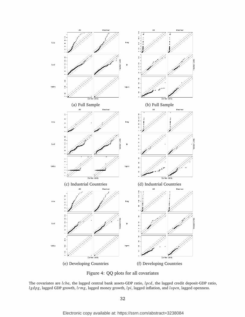
of each covariate graphically in Figure 4 for all samples. The covariates are lcba, the lagged
central bank assets-GDP ratio, l pcd, the lagged credit deposit-GDP ratio, l gdpg, lagged GDP
growth, l rmg, lagged money growth, l pi, lagged inflation, and lopen, lagged openness. If the
empirical distributions are the same for targeters and non-targeters, the points in the Q-Q plots
lie on the 45 degree line. Deviations from it imply differences in the empirical distribution. As
shown in these plots, matching would improve the empirical distribution for lagged openness
and lagged GDP growth in the full sample.
The results of the average treatment effect on the treated using parametric propensity scores
are presented in Table 6. In all samples, the ATTs on inflation is negative, but not statistically
significant. The ATT estimates using the parametric model are different than those estimated by
the semiparametric model. The contrast signifies the impact of propensity score misspecification
on the ATTs. Other results supporting our view are the estimates on the sacrifice ratio, inflation
variability, and interest rate volatility. The average treatment effect on the treated on inflation
variability is negative across different country groups and coefficients are statistically significant
29

Electronic copy available at: https://ssrn.com/abstract=3238084
0
1
2
3
0.25 0.50 0.75 1.00Propensity Score
de
nsity
Control Treated
(a) Full Sample
0
1
2
3
0.25 0.50 0.75 1.00Propensity Score
de
nsity
Control Treated
(b) Industrial Economies
0
1
2
3
0.25 0.50 0.75Propensity Score
de
nsity
Control Treated
(c) Developing Countries
Figure 2: Kernel densities of the estimated probit propensity scores
in the full sample and developing subsamples.
Table 6: Average treatment effect on the treated, probit propensityscores
π debt SR σπ σi σs
FULL -0.70 -21.29∗∗∗ -0.06 -1.88∗∗∗ -1.22∗∗∗ -1.53∗∗∗
(0.97) (2.23) (0.15) (0.67) (0.34) (0.6)
IND -0.05 -33.9∗∗∗ -0.2 -0.16 -0.06 1.77∗∗∗
(0.23) (3.49) (0.3) (0.14) (0.19) (0.48)
DCS -0.72 -11.68∗∗∗ -0.02 -1.93∗∗ -0.68 -2.01∗∗
(1.51) (2.78) (0.18) (0.98) (0.47) (0.81)
Outcomes are inflation (π), the debt-GDP ratio (debt) as a proxy for fiscaldiscipline, the sacrifice ratio (SR) measured by the change in output to thechange in inflation, inflation variability (σπ), interest rate volatility (σi),and exchange rate volatility (σs). Volatilities are measured by the standarddeviation of a three-year moving average.FULL: the full sample, IND: industrial economies, DCS: developing countries.∗p<0.1; ∗∗p<0.05; ∗∗∗p<0.01.
The sign of treatment effects on fiscal discipline and exchange rate volatility are similar
compared to the index results, but the magnitudes are different. The effects of IT on inflation,
inflation variability, the sacrifice ratio, and interest rate volatility are inconsistent. The results
suggest the choice of propensity scores has a considerable impact on the treatment effect
estimates. Our empirical study suggests that the single index coefficient regression model in
30

Electronic copy available at: https://ssrn.com/abstract=3238084
Raw Treated
Propensity Score
Den
sity
0.0 0.2 0.4 0.6 0.8 1.0
0.0
0.5
1.0
1.5
2.0
2.5
Matched Treated
Propensity Score
Den
sity
0.0 0.2 0.4 0.6 0.8 1.00.
00.
51.
01.
52.
02.
5
Raw Control
Propensity Score
Den
sity
0.0 0.2 0.4 0.6 0.8 1.0
0.0
1.0
2.0
3.0
Matched Control
Propensity Score
Den
sity
0.0 0.2 0.4 0.6 0.8 1.0
0.0
0.5
1.0
1.5
2.0
2.5
Freq
uenc
y of
Pro
pens
ity S
core
Freq
uenc
y of
Pro
pens
ity S
core
Freq
uenc
y of
Pro
pens
ity S
core
Freq
uenc
y of
Pro
pens
ity S
core
Figure 3: Histograms of the estimated propensity scores before and after matching
31
Electronic copy available at: https://ssrn.com/abstract=3238084
(a) Full Sample (b) Full Sample
(c) Industrial Countries (d) Industrial Countries
(e) Developing Countries (f) Developing Countries
Figure 4: QQ plots for all covariates
The covariates are lcba, the lagged central bank assets-GDP ratio, l pcd, the lagged credit deposit-GDP ratio,l gdpg, lagged GDP growth, l rmg, lagged money growth, l pi, lagged inflation, and lopen, lagged openness.
32

Electronic copy available at: https://ssrn.com/abstract=3238084
conjunction with the proposed estimation method could be useful in propensity score analysis.
5 Sensitivity Analysis
A vast literature uses parametric propensity score matching to examine the effectiveness of
inflation targeting. The sensitivity analysis determines whether the results from our proposed
semiparametric approach are robust to various scenarios. As a robustness check, we report the
results of the first and second stages when the conventional covariates are used. Conventional
covariates are macroeconomic predictors in which the preconditions are not included. We also
compare the ATTs when the contemporaneous variables are used in the first stage. Our last
comparison involves propensity score models for the pre-crisis period.
5.1 Conventional Covariates
One of the contributions of this paper is to include preconditions in the estimation of
propensity scores. Existing studies such as Lin and Ye (2007) estimate propensity scores based
only upon macroeconomic predictors. In the previous sections, we show how preconditions
affect the likelihood of the IT adoption. We compare our results to the literature by estimating
propensity scores with conventional covariates. Table B3 summarizes the results of the first-stage
estimation using the conventional covariates. The set of the conventional covariates includes
lagged GDP growth, lagged money growth, lagged inflation, and pegged exchange. Tables 7
and 8 include treatment effects of IT using the single index and probit propensity scores.
The comparison of Table 7 with Table 3 implies the ATTs on inflation using the conventional
covariates in the first stage differs from the results using all the variables. This holds true for
the sacrifice ratio in the full and developing samples, inflation variability for the full sample,
and interest rate volatility in the developing sample. The findings in this section signify the role
of preconditions.
33

Electronic copy available at: https://ssrn.com/abstract=3238084
Table 7: Average treatment on the treated, index propensity scoreswith conventional covariates
π debt SR σπ σi σs
FULL 0.27 -13.92∗∗∗ 0.04 -0.34 -1.05∗∗∗ -2.36∗∗∗
(0.85) (2.13) (0.15) (0.54) (0.32) (0.64)
IND -0.23 -29.41∗∗∗ -1.44∗∗∗ -0.14 -0.74∗∗∗ 1.13∗∗
(0.19) (2.85) (0.29) (0.13) (0.29) (0.55)
DCS -0.11 -9.98∗∗∗ -0.04 -0.72 -0.61 -1.67∗
(1.56) (2.65) (0.17) (0.92) (0.46) (0.86)
Outcomes are inflation (π), the debt-GDP ratio (debt) as a proxy for fiscaldiscipline, the sacrifice ratio (SR) measured by the change in output to thechange in inflation, inflation variability (σπ), interest rate volatility (σi),and exchange rate volatility (σs). Volatilities are measured by the standarddeviation of a three-year moving average.FULL: the full sample, IND: industrial economies, DCS: developing countries.∗p<0.1; ∗∗p<0.05; ∗∗∗p<0.01.
Table 8: Average treatment on the treated, probit propensity scoreswith conventional covariates
π debt SR σπ σi σs
FULL -0.88 -15.92∗∗∗ -0.08 -1.33∗∗ -1.81∗∗∗ -2.47∗∗∗
(0.88) (2.03) (0.16) (0.59) (0.34) (0.61)
IND -0.02 -34.85∗∗∗ 0.01 0.02 -0.32 1.75∗∗∗
(0.16) (3.45 ) (0.29) (0.11) (0.24) (0.51)
DCS -1.11 -13.96∗∗∗ -0.04 -1.45∗ -1.18∗∗ -2.32∗∗∗
(1.53) (2.58) (0.18) (0.87) (0.47) (0.82)
Outcomes are inflation (π), the debt-GDP ratio (debt) as a proxy for fiscaldiscipline, the sacrifice ratio (SR) measured by the change in output to thechange in inflation, inflation variability (σπ), interest rate volatility (σi),and exchange rate volatility (σs). Volatilities are measured by the standarddeviation of a three-year moving average.FULL: the full sample, IND: industrial economies, DCS: developing countries.∗p<0.1; ∗∗p<0.05; ∗∗∗p<0.01.
34

Electronic copy available at: https://ssrn.com/abstract=3238084
5.2 Lagged vs. Contemporaneous Covariates
The literature on treatment effects of IT lacks a rigorous explanation of endogeneity. Gertler
(2005) points to the endogeneity problem in examining whether IT is effective. He explains
the difficulties of identifying its effects have been raised by Ball and Sheridan (2003) and
Mishkin and Schmidt-Hebbel (2007). The use of lagged covariates has been proposed as a
partial solution to this problem. In order to consider the lag in the effect IT, we model the
likelihood of IT using lagged covariates. However, some studies estimate the propensity score
using contemporaneous variables. This section shows the robustness of our findings to the use
of contemporaneous covariates.
Table B3 summarizes the first stage estimations using the single index model with
contemporaneous variables. Tables 9 and 10 present the average treatment effect on the
treated using corresponding variables and methods. The treatment effects on all variables
considering contemporaneous variables are similar to the treatment effects from the baseline
model suggesting the robustness of our results to the use of contemporaneous covariates. The
point estimates, however, are different. For example, as compared to the baseline model we
find that IT leads to reduction in inflation, inflation volatility and interest rate volatility, though
these effects are insignificant for the developing economies. Comparing Table 10 with Table 6
shows that the treatment effects are not sensitive to the choice of variables in case of parametric
specification except interest rate volatility where the effect is significantly negative in the case
of conventional covariates. Consistent with the comparison of the semiparametric model with
the parametric model in the case of the baseline model, we also find differences in the results
when we use conventional variables. For example, using parametric propensity score, we find
that the treatment effect on inflation volatility is negative and statistically significant.
35

Electronic copy available at: https://ssrn.com/abstract=3238084
Table 9: Average treatment on the treated, index propensity scoreswith the contemporaneous covariates
π debt SR σπ σi σs
FULL 0.77 -15.34∗∗∗ 0.01 -0.6 -0.82∗∗∗ -2.06∗∗∗
(0.81) (2.11) (0.15) (0.55) (0.32) (0.61)
IND -0.13 -39.69∗∗∗ -0.78∗∗∗ -0.1 -0.31 0.96∗∗
(0.21) (3.25) (0.31) (0.13) (0.23) (0.48)
DCS 1.43 0.26 0.07 0.35 -0.18 -1.73∗∗
(1.29) (2.53) (0.17) (0.79) (0.45) (0.83)
Outcomes are inflation (π), the debt-GDP ratio (debt) as a proxy for fiscaldiscipline, the sacrifice ratio (SR) measured by the change in output to thechange in inflation, inflation variability (σπ), interest rate volatility (σi),and exchange rate volatility (σs). Volatilities are measured by the standarddeviation of a three-year moving average.FULL: the full sample, IND: industrial economies, DCS: developing countries.∗p<0.1; ∗∗p<0.05; ∗∗∗p<0.01.
Table 10: Average treatment on the treated, probit propensityscores with contemporaneous variables
π debt SR σπ σi σs
FULL 0.39 -17.68∗∗∗ -0.09 -1.13∗∗ -1.2∗∗∗ -1.37∗∗
(0.88) (2.14) (0.16) (0.56) (0.33) (0.58)
IND -0.04 -32.71∗∗∗ -0.37 -0.16 0.01 2.07∗∗
(0.22) (3.27) (0.33) (0.15) (0.18) (0.47)
DCS -0.2 -12.42∗∗∗ 0.07 -1.71 -0.55 -1.85∗∗
(1.51) (2.72) (0.18) (1.00) (0.48) (0.81)
Outcomes are inflation (π), the debt-GDP ratio (debt) as a proxy for fiscaldiscipline, the sacrifice ratio (SR) measured by the change in output tothe change in inflation, inflation variability (σπ), interest rate volatility(σi), and exchange rate volatility (σs). Volatilities are measured by thestandard deviation of a three-year moving average.FULL: the full sample, IND: industrial economies, DCS: developingcountries.∗p<0.1; ∗∗p<0.05; ∗∗∗p<0.01.
36
Electronic copy available at: https://ssrn.com/abstract=3238084
5.3 Pre-crisis Period
The empirical work on the IT effectiveness has considered a sample period before the global
financial crisis (Ball and Sheridan (2003), Lin and Ye (2007), Lucotte (2012), and Lin and Ye
(2013)). Our sample period of 1990–2013 includes years after the crisis. In this section we
consider whether our results are sensitive to the inclusion of the crisis and the post-crisis time
periods by estimating the model for the pre-crisis period (1990–2007). Table B4 summarizes
the results of the first stage using conventional variables for the pre-crisis period. We exclude
the lagged central bank assets ratio and the lagged credit deposit-GDP ratio. The findings of the
second stage estimation, Table 11, indicate the effect of IT on fiscal discipline remains unchanged
prior to the crisis which is consistent with our previous findings. We interpret these robust
results as evidence for the causal role of inflation targeting per se on fiscal discipline. Inflation
variability has decreased in all targeters in the pre-crisis period. However, the coefficient is not
statistically significant. The treatment effects on interest rate volatility remain the same before
the crisis. The findings presented in Table 11 and the comparison with the full sample period
(Table 3) determine our main findings are not sensitive to the post-crisis period.
Lin and Ye (2007) also referred to the selection problem, but their approach is estimating
the propensity scores parametrically. They use a sample of 22 industrial countries over the
period 1985–1999. Our Table 12 presents the results most comparable to those of Lin and
Ye (2007).11 Their ATTs on inflation for the constant and non-constant inflation targeting
frameworks are -0.002 and -0.0034. The ATTs are not statistically significant. We find the ATT
on inflation for industrial countries -0.88 which is statistically significant at the one percent level.
Their treatment effects on inflation variability are -0.0003 and 0.0009 and are not statistically
significant. Our treatment effect on inflation variability is -2.93 and statistically significant at
the one percent level. This discrepancy is the result of using a misspecified propensity score
model.
Table 12 summarizes the average treatment on the treated, index propensity scores with
11See Tables 3 and 4 in P. 2528 of Lin and Ye (2007).
37

Electronic copy available at: https://ssrn.com/abstract=3238084
Table 11: Average treatment on the treated, single index propensityscores with conventional covariates (pre-crisis periods)
π debt SR σπ σi σs
FULL -0.10 -14.94∗∗∗ 0.08 -0.94 -0.63∗ -2.37∗∗∗
(1.26) (2.4) (0.16) (0.80) (0.37) (0.76)
IND -0.49∗∗ -33.72∗∗∗ -1.26∗∗∗ -0.11 -1.26∗∗∗ -0.27(0.21) (3.65) (0.32) (0.14) (0.36) (0.84)
DCS 0.94 -5.60∗ 0.10 -0.91 0.20 -0.95(1.86) (3.25) (0.18) (1.23) (0.50) (1.02)
FULL: the full sample, IND: industrial economies, DCS: developing countries.∗p<0.1; ∗∗p<0.05; ∗∗∗p<0.01.
contemporaneous covariates for the pre-crisis periods. We find that fiscal discipline is robust to
the contemporaneous variables.
Table 12: Average treatment on the treated, single index propensityscores with contemporaneous covariates (pre-crisis periods)
π debt SR σπ σi σs
FULL 1.72 -15.6∗∗∗ 0.06 0.32 -0.37 -0.88(1.08) (2.46) (0.15) (0.66) (0.37) (0.72)
IND -0.88∗∗∗ -21.72∗∗∗ -1.15∗∗∗ -2.93∗∗∗ -0.51∗ 2.71∗∗∗
(0.25) (3.00) (0.28) (0.47) (0.29) (0.57)
DCS 3.41∗∗ -4.11 -0.21 0.07 0.37 -1.32(1.65) (3.38) (0.18) (1.10) (0.51) (0.89)
FULL: the full sample, IND: industrial economies, DCS: developing countries.∗p<0.1; ∗∗p<0.05; ∗∗∗p<0.01.
6 Concluding Remarks
The purpose of this paper is to examine the causal effect of IT adoption on macroeconomic
performance using a semiparametric index model. The semiparametric index model takes into
account the model misspecification in the parametric estimation of the propensity scores and the
38

Electronic copy available at: https://ssrn.com/abstract=3238084
“curse of dimensionality” problem associated with the nonparametric model. We also consider
the prominent role of preconditions in IT adoption by including the central bank assets-GDP
ratio and the private credit-GDP ratio in the first stage estimations of the probability of adoption
of IT. In addition to examining the impact on level of inflation and inflation volatility, we also
estimate the treatment effect on volatility of interest rate and exchange rate, sacrifice ratio and
the debt-GDP ratio. This provides us a measure of the indirect effect of IT.
We find that the treatment effects on inflation and inflation volatility are statistically
insignificant for both the developed and the developing economies. This result is in contrast
to the parametric propensity scores that suggest significant decline in inflation volatility in
developing countries. The results from the semiparametric model also suggest a decline in
sacrifice ratio and interest rate volatility for the developed country inflation targeters, whereas
the impact is insignificant in case of developing economies. The adoption of IT leads to an
increase in volatility of exchange rate in developed economies, but it reduces the exchange rate
volatility in developing economies. Our results show that adoption of IT leads to improvement
in debt-GDP ratio in both the developed and the developing economies. Our findings are also
robust to the use of conventional covariates in the first stage, and a smaller sample period
(before the 2008 financial crisis). We find that the method used to estimate propensity scores
influences the treatment effect estimates and the semiparametric propensity score provides
efficient and consistent estimates.
Acknowledgements
We thank two referees for their constructive comments which led to improvements in the
paper and the Co-editor, James Bullard, for guidance on advancement of this article.
References
Amato, J. D., and S. Gerlach. 2002. “Inflation targeting in emerging market and transitioneconomies: Lessons after a decade.” European Economic Review, 46(4-5): 781–790.
39
Electronic copy available at: https://ssrn.com/abstract=3238084
Angeriz, A., and P. Arestis. 2007. “Assessing the performance of ‘inflation targeting lite’countries.” The World Economy, 30(11): 1621–1645.
Ball, L., and N. Sheridan. 2003. “Does inflation targeting matter?” The Inflation TargetingDebate. University of Chicago Press.
Bernanke, B., and M. Woodford. 2005. The Inflation-Targeting debate. Vol. 32, Chicago andLondon:University of Chicago Press.
Brito, R. 2010. “Inflation targeting does not matter: another look at OECD sacrifice ratios.”Journal of Money, Credit, and Banking, 42(8): 1679–1688.
Buuren, S., and K. Groothuis-Oudshoorn. 2011. “MICE: Multivariate imputation by chainedequations in R.” Journal of Statistical Software, 45(3).
Chadha, J. S., and C. Nolan. 2001. “Inflation targeting, transparency and interest rate volatility:ditching ‘monetary mystique’ in the UK.” Journal of Macroeconomics, 23: 349–366.
Creel, J., and P. Hubert. 2010. “Has inflation targeting changed the conduct of monetarypolicy?” Macroeconomic Dynamics, FirstView: 1–21.
Dehejia, R. H., and S. Wahba. 1999. “Causal effects in nonexperimental studies: reevaluatingthe evaluation of training programs.” Journal of the American Statistical Association,94: 1053–1062.
Dehejia, R. H., and S. Wahba. 2002. “Propensity score-matching methods for nonexperimentalcausal studies.” The Review of Economics and Statistics, 84: 151–161.
de Mendonca, H. F., and G. J. de Guimaraes. 2012. “Is inflation targeting a good remedy tocontrol inflation?” Journal of Development Economics, 98(2): 178–191.
Demertzis, M., and A. H. Hallett. 2007. “Central bank transparency in theory and practice.”Journal of Macroeconomics, 29(4): 760–789.
Edwards, S. 2006. “The relatioship between exchange rates and inflation targeting revisited.”National Bureau of Economic Research.
Eo, Y., and D. Lie. 2017. “The role of the inflation target adjustment in stabilization policy.”Economics Working Paper Series, 1–40.
Filho, I. 2011. “28 months later: how inflation targeters outperformed their peers in the greatrecession.” The BE Journal of Macroeconomics, 11(1).
Gertler, M. 2005. “Comment on ‘Does Inflation Targeting Matter?’.” The Inflation TargetingDebate, 276–281.
Goncalves, C. E., and A. Carvalho. 2009. “Inflation targeting matters: evidence from OECDeconomies’ Sacrifice Ratios.” Journal of Money, Credit, and Banking, 41(1): 233–243.
40

Electronic copy available at: https://ssrn.com/abstract=3238084
Gregorio, J., A. Tokman, and R. Valdés. 2005. “Flexible exchange rate with inflation targetingin Chile: Experience and issues.” Working Paper, Inter-American Development Bank, ResearchDepartment.
Hardle, W., P. Hall, and H. Ichimura. 1993. “Optimal smoothing in single index models.” Theannals of Statistics, 21: 157–178.
Hayfield, T., and J. S. Racine. 2008. “Nonparametric econometrics: The np package.” Journalof Statistical Software, 27(5): 1–32.
Hirano, K., G. W. Imbens, and G. Ridder. 2003. “Efficient estimation of average treatmenteffects using the estimated propensity score.” Econometrica, 71(4): 1161–1189.
Ichimura, H. 1993. “Semiparametric least squares (SLS) and weighted SLS estimation.” Journalof Econometrics, 58(1-2): 71–120.
Ichimura, H., and P. E. Todd. 2007. “Implementing nonparametric and semiparametricestimators.” Handbook of Econometrics, 6: 5369–5468.
Ilzetzki, E., C. M. Reinhart, and K. S. Rogoff. 2008. “Exchange rate arrangements enteringthe 21st century: Which anchor will hold?” University of Maryland and Harvard University.
Johnson, D. R. 2002. “The effect of inflation targeting on the behavior of expected inflation:evidence from an 11 country panel.” Journal of Monetary Economics, 49(8): 1521–1538.
Klein, R. W., and R. H. Spady. 1993. “An efficient semiparametric estimator for binary responsemodels.” Econometrica, 61: 387–421.
Lin, S. 2010. “On the international effects of inflation targeting.” The Review of Economics andStatistics, 92(1): 195–199.
Lin, S., and H. Ye. 2007. “Does inflation targeting really make a difference? Evaluating thetreatment effect of inflation targeting in seven industrial countries.” Journal of MonetaryEconomics, 54(8): 2521–2533.
Lin, S., and H. Ye. 2013. “Does Inflation Targeting Help Reduce Financial Dollarization?”Journal of Money, Credit and Banking, 45(7): 1253–1274.
Li, Q., and J. S. Racine. 2011. Nonparametric econometrics: Theory and practice. PrincetonUniversity Press.
Lucotte, Y. 2012. “Adoption of inflation targeting and tax revenue performance in emergingmarket economies: An empirical investigation.” Economic Systems, 36(4): 609–628.
Minea, A., and R. Tapsoba. 2014. “Does inflation targeting improve fiscal discipline?” Journalof International Money and Finance, 40: 185–203.
Mishkin, F. S., and K. Schmidt-Hebbel. 2001. “One decade of inflation targeting in the world:What do we know and what do we need to know?” National Bureau of Economic Research.
41

Electronic copy available at: https://ssrn.com/abstract=3238084
Mishkin, F. S., and K. Schmidt-Hebbel. 2007. “Does inflation targeting make a difference?”National Bureau of Economic Research.
Mishkin, F. S., and M. A. Savastano. 2001. “Monetary policy strategies for Latin America.”Journal of Development Economics, 66(2): 415–444.
Morris, S., and H. S. Shin. 2002. “Social value of public information.” The American EconomicReview, 92(5): 1521–1534.
Neumann, M. J., and J. von Hagen. 2002. “Does inflation targeting matter?” ZEI WorkingPaper.
Romer, D. 1993. “Openness and inflation: Theory and evidence.” Quarterly Journal of Economics,108(4): 869–903.
Rose, A. K. 2007. “A stable international monetary system emerges: Inflation targeting isBretton Woods, reversed.” Journal of International Money and Finance, 26(5): 663–681.
Rosenbaum, P. R., and D. B. Rubin. 1983. “The central role of the propensity score inobservational studies for causal effects.” Biometrika, 70(1): 41–55.
Samarina, A., M. Terpstra, and J. De Haan. 2013. “Inflation targeting and inflationperformance: a comparative analysis.” Applied Economics, 46(1): 41–56.
Song, K. 2014. “Semiparametric models with single-index nuisance parameters.” Journal ofEconometrics, 178: 471–483.
Stone, C. J. 1980. “Optimal rates of convergence for nonparametric estimators.” The annals ofStatistics, 8(6): 1348–1360.
Svensson, L. E. 1996. “Inflation forecast targeting: Implementing and monitoring inflationtargets.” European Economic Review, 41(6): 1111–1146.
Svensson, L. E. 1999. “Inflation targeting as a monetary policy rule.” Journal of MonetaryEconomics, 43(3): 607–654.
Svensson, L. E. 2005a. “Optimal inflation targeting: Further developments of inflationtargeting.” Sveriges Riksbank Conference,‘Inflation Targeting: Implementation, Communication,and Effectiveness’.
Svensson, L. E. 2005b. “Social value of public information: Morris and Shin (2002) is actuallypro-transparency, not con.” National Bureau of Economic Research.
Vega, M., and D. Winkelried. 2005. “Inflation targeting and inflation behavior: a successfulstory?” International Journal of Central Banking, 1(3): 153–175.
Woodford, M. 2005. “Central bank communication and policy effectiveness.” National Bureauof Economic Research.
42

Electronic copy available at: https://ssrn.com/abstract=3238084
Wu, T. Y. 2004. “Does inflation targeting reduce? inflation? An analysis for the OECD industrialcountries.” Working Paper Series.
Zhao, Z. 2008. “Sensitivity of propensity score methods to the specifications.” Economics Letters,98(3): 309–319.
Appendix A
Table A1 provides the list of inflation targeting countries along with the adoption dates,
target level at the adoption date and their country groups, whether the country is developed or
developing. Table A2 presents the control units and their country groups. The first country that
has adopted explicit inflation targeting is New Zealand with the target rate of 4 percent at the
adoption date and the last one is Serbia with the target rate of 8 percent in 2006Q3.
43

Electronic copy available at: https://ssrn.com/abstract=3238084
Table A1: Treated group (targeters): adoption date,target level at the adoption date, and country group
Countries Adoption Date Target Group
Armenia 2006Q1 4 DCSAustralia 1993Q2 3 INDBrazil 1999Q2 8 DCSCanada 1991Q1 4 INDChile 1999Q3 3 DCSColombia 1999Q3 5 DCSCzech 1997Q4 6 INDGhana 2002Q1 12 DCSGuatemala 2005Q1 5 DCSHungary 2001Q2 7 DCSIceland 2001Q1 4 INDIndonesia 2005Q3 5 DCSIsrael 1992Q1 15 INDMexico 2001Q1 5 DCSNew Zealand 1989Q4 4 INDNorway 2001Q1 3 INDPeru 2002Q1 3 DCSPhilippines 2002Q1 5 DCSPoland 1998Q1 8 DCSRomania 2005Q3 8 DCSSerbia 2006Q3 8 DCSSouth Africa 2000Q1 3 DCSSouth Korea 1998Q2 9 INDSweden 1993Q1 2 INDThailand 2000Q2 2 DCSTurkey 2006Q1 5 DCSUK 1992Q3 3 IND
DCS denotes developing countries and IND indicatesindustrial economies.
44

Electronic copy available at: https://ssrn.com/abstract=3238084
Table A2: Control group (non-targeters)
Countries Group Countries Group
Albania DCS Madagascar DCSAlgeria DCS Malawi DCSArgentina DCS Malaysia DCSArmenia DCS Maldives DCSAustria IND Mali DCSAzerbaijan DCS Malta INDBelarus DCS Moldova DCSBelgium DCS Morocco DCSBelize DCS Mozambique DCSBolivia DCS Myanmar DCSBulgaria DCS Nepal DCSChina DCS Netherlands INDCosta Rica DCS Nicaragua DCSCyprus IND Niger DCSDenmark IND Saudi Arabia DCSEcuador DCS Senegal DCSEgypt DCS Singapore INDEl Salvador DCS Slovenia INDEstonia DCS Spain INDFiji DCS Sri Lanka DCSFrance IND Sudan DCSGermany IND Swaziland DCSGreece IND Tanzania DCSIndia DCS Tunisia DCSIran DCS Uganda DCSIreland IND Ukraine DCSItaly IND United Arab Emirates DCSJamaica DCS United States INDJapan IND Uruguay DCSJordan DCS Vanuatu DCSKazakhstan DCS Venezuela DCSKenya DCS Vietnam DCSLebanon DCS Yemen DCSLibya DCS Zambia DCSLuxembourg IND Zimbabwe DCSMacedonia DCS
DCS denotes developing countries and IND indicates industrialeconomies.
45

Electronic copy available at: https://ssrn.com/abstract=3238084
Appendix B
Appendix B summarizes the first stage estimates.
Nonparametric Propensity Scores
Table B1 includes the results of the nonparametric series estimates proposed by Hirano,
Imbens and Ridder (2003). The variables in Table B1 are defined as follows: X1 is lagged
openness. X2 is lagged GDP growth. X3 indicates lagged real money growth. X4 is lagged
inflation. X5 denotes the pegged exchange regime dummy. X6 and X7 represent lagged CB
assets-GDP and lagged private credit-GDP, respectively. Our model consists of 35 covariates
including the second powers and their interaction terms. The estimation is stopped at the
second power, because standard errors become very large, causing instability in the estimates
of the coefficients.
Parametric Propensity Scores
The results of the probit model are presented in Table B2. We also estimate the propensity
score using a logit model. The estimates are similar to probit. The response variable is the
targeting dummy and takes the value of 1 if the country adopts inflation targeting. In the
first stage estimation of treatment effects, we include both institutional characteristics and
macroeconomic predictors to estimate the likelihood of adopting IT. We find a statistically
significant and negative relation between openness and the likelihood of adopting IT for the full
sample, industrial economies and developing countries. A higher degree of openness lowers
the probability of adopting IT. As pointed out by Romer (1993), more open economies are
less likely to adopt inflation targeting. Under monetary expansion, the real exchange rate
depreciates. Since the harms of real depreciation are greater in more open economies, the
degree of openness and the benefits of expansion are inversely related. Moreover, GDP growth
lowers the probability of the IT adoption.
46

Electronic copy available at: https://ssrn.com/abstract=3238084
Table B1: Nonparametric series models for the full, industrial, and developingsamples
Covariates FULL IND DCS Covariates FULL IND DCS
X1 −0.018∗∗∗ −0.021∗∗∗ −0.023∗∗∗ X4X5 0.009 0.056 0.023∗∗
(0.004) (0.007) (0.005) (0.006) (0.142) (0.009)
X 21 −0.00002 −0.00004 0.00005∗∗∗ X 2
5 0.0003 0.001 0.004(0.00002) (0.00003) (0.00002) (0.0002) (0.01) (0.003)
X2 −0.293∗∗∗ −0.245 −0.308 X6 −0.060∗∗∗ −0.145∗∗ −0.046∗∗∗
(0.065) (0.244) (0.271) (0.013) (0.057) (0.016)
X1X2 −0.0001 −0.0004 0.008∗∗∗ X1X6 0.0002 −0.00005 0.0002∗
(0.001) (0.002) (0.003) (0.0001) (0.0004) (0.0001)
X 22 −0.057∗∗∗ 0.020 −0.958∗∗∗ X2X6 0.005∗∗ 0.016 −0.008
(0.007) (0.017) (0.097) (0.002) (0.010) (0.007)
X3 −0.020 0.091∗ −0.040∗ X3X6 −0.0001 −0.005 −0.0002(0.014) (0.047) (0.023) (0.001) (0.003) (0.001)
X1X3 0.00005 −0.001∗ 0.001∗∗ X4X6 −0.0002 0.001 0.0001(0.0002) (0.0005) (0.0003) (0.0004) (0.005) (0.001)
X2X3 −0.005∗ −0.029 −0.025∗∗ X5X6 0.019∗∗∗ 0.058 0.017∗∗
(0.003) (0.019) (0.012) (0.006) (0.040) (0.007)
X 23 0.0002∗ 0.0002 0.0001 X 2
6 0.001∗∗∗ 0.002∗ 0.001∗∗∗
(0.0001) (0.0002) (0.0001) (0.0001) (0.001) (0.0001)
X4 −0.014 −0.084 −0.027∗∗ X7 0.018∗∗∗ −0.005 0.024∗∗∗
(0.010) (0.161) (0.014) (0.003) (0.007) (0.007)
X1X4 0.0001 −0.003∗ 0.0001 X1X7 0.0001∗∗∗ 0.0001∗∗ 0.00002(0.0001) (0.001) (0.0001) (0.00003) (0.00005) (0.00005)
X2X4 0.004∗∗∗ −0.029 0.009 X2X7 −0.0001 0.0002 −0.017∗∗∗
(0.001) (0.029) (0.007) (0.001) (0.002) (0.003)
X3X4 −0.00001 −0.004 −0.0001 X3X7 0.0002 0.0001 −0.00001(0.0001) (0.004) (0.0003) (0.0001) (0.0004) (0.0003)
X 24 0.0001 −0.002 0.0002∗∗ X4X7 −0.0001 0.004∗∗∗ −0.0003∗∗∗
(0.00004) (0.002) (0.0001) (0.0001) (0.001) (0.0001)
X5 −0.740∗∗∗ −1.600∗∗∗ −0.390 X5X7 −0.005∗∗∗ −0.007∗ −0.010∗∗
(0.178) (0.522) (0.298) (0.002) (0.004) (0.005)
X1X5 0.004 0.014∗∗∗ −0.004 X6X7 −0.0002 0.0004 −0.001∗∗
(0.002) (0.005) (0.004) (0.0001) (0.0004) (0.0002)
X2X5 0.087 0.003 0.013 X 27 −0.0001∗∗∗ −0.00004 −0.00001
(0.055) (0.165) (0.202) (0.00002) (0.00003) (0.0001)
X3X5 −0.004 0.031 0.010(0.011) (0.035) (0.018)
Observations 2,352 624 1,728Log Likelihood −993.626 −263.836 −487.513Akaike Inf. Crit. 2,057.253 597.673 1,045.027
X1: lagged openness, X2: lagged GDP growth, X3: lagged real money growth, X4: laggedinflation, X5: pegged exchange regime dummy, X6: lagged CB asset to GDP, X7: lagged privatecredit to GDP.∗p<0.1; ∗∗p<0.05; ∗∗∗p<0.01.
47

Electronic copy available at: https://ssrn.com/abstract=3238084
Table B2: Probit models for the full sample, industrial, anddeveloping countries
FULL IND DCS
Lagged Openness −0.010∗∗∗ −0.008∗∗∗ −0.010∗∗∗
(0.001) (0.001) (0.001)
Lagged GDP Growth −0.090∗∗∗ −0.168∗∗∗ −0.082∗∗∗
(0.015) (0.055) (0.016)
Lagged Money Growth 0.006∗∗∗ 0.023∗∗ 0.004∗∗∗
(0.001) (0.011) (0.001)
Lagged Inflation −0.003∗ 0.022 −0.003∗
(0.002) (0.017) (0.002)
Pegged Exchange Regime −0.402∗∗∗ −0.159 −0.472∗∗∗
(0.056) (0.114) (0.068)
Lagged CB Assets 0.002 −0.015 0.004∗
(0.002) (0.009) (0.002)
Lagged Credit Deposit 0.008∗∗∗ 0.005∗∗∗ 0.009∗∗∗
(0.001) (0.001) (0.001)
Observations 2,352 624 1,728Log Likelihood −1,165.593 −328.671 −821.601Akaike Inf. Crit. 2,345.186 671.342 1,657.201
The dependent variable is the targeting dummy, which has the value 1 if thecountry adopts inflation targeting.∗p<0.1; ∗∗p<0.05; ∗∗∗p<0.01.
48
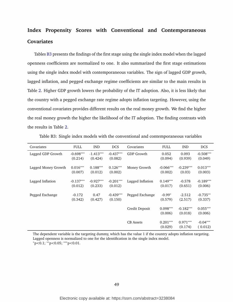
Electronic copy available at: https://ssrn.com/abstract=3238084
Index Propensity Scores with Conventional and Contemporaneous
Covariates
Tables B3 presents the findings of the first stage using the single index model when the lagged
openness coefficients are normalized to one. It also summarized the first stage estimations
using the single index model with contemporaneous variables. The sign of lagged GDP growth,
lagged inflation, and pegged exchange regime coefficients are similar to the main results in
Table 2. Higher GDP growth lowers the probability of the IT adoption. Also, it is less likely that
the country with a pegged exchange rate regime adopts inflation targeting. However, using the
conventional covariates provides different results on the real money growth. We find the higher
the real money growth the higher the likelihood of the IT adoption. The finding contrasts with
the results in Table 2.
Table B3: Single index models with the conventional and contemporaneous variables
Covariates FULL IND DCS Covariates FULL IND DCS
Lagged GDP Growth -0.698∗∗∗ -1.413∗∗∗ -0.437∗∗∗ GDP Growth 0.052 0.093 -0.508∗∗∗
(0.214) (0.424) (0.082) (0.094) (0.939) (0.049)
Lagged Money Growth 0.016∗∗∗ 0.188∗∗∗ 0.126∗∗∗ Money Growth -0.066∗∗∗ -0.239∗∗∗ 0.013∗∗∗
(0.007) (0.012) (0.002) (0.002) (0.03) (0.003)
Lagged Inflation -0.137∗∗∗ -0.927∗∗∗ -0.201∗∗∗ Lagged Inflation 0.149∗∗∗ -0.578 -0.189∗∗∗
(0.012) (0.233) (0.012) (0.017) (0.651) (0.006)
Pegged Exchange -0.172 0.47 -0.439∗∗∗ Pegged Exchange -0.99∗ -2.512 -0.735∗∗
(0.342) (0.427) (0.150) (0.579) (2.517) (0.337)
Credit Deposit 0.098∗∗∗ -0.182∗∗∗ 0.055∗∗∗
(0.006) (0.018) (0.006)
CB Assets 0.201∗∗∗ 0.971∗∗∗ -0.04∗∗∗
(0.029) (0.174) ( 0.012)
The dependent variable is the targeting dummy, which has the value 1 if the country adopts inflation targeting.Lagged openness is normalized to one for the identification in the single index model.∗p<0.1; ∗∗p<0.05; ∗∗∗p<0.01.
49

Electronic copy available at: https://ssrn.com/abstract=3238084
The Pre-Crisis Period
Table B4 summarizes the results of the first stage using conventional and contemporaneous
variables for the pre-crisis period. We exclude the lagged central bank assets ratio and the
lagged credit deposit-GDP ratio.
Table B4: Single index models with the conventional and contemporaneous covariates, (pre-crisisperiods)
FULL IND DCS FULL IND DCS
Lagged GDP Growth -1.752∗∗∗ -0.987 -0.48∗∗ -2.558∗∗∗ -0.247∗∗ -0.364∗∗∗
(0.357) (1.029) (0.201) (0.204) (0.129) (0.128)
Lagged Money Growth 0.053∗∗∗ -0.872∗∗∗ 0.029∗∗∗ 0.03∗∗∗ -0.004 -0.046∗∗∗
(0.01) (0.132) (0.009) (0.009) (0.003) (0.005)
Lagged Inflation 0.101∗∗∗ -0.916∗∗∗ -0.373∗∗∗ 0.019 0.005 -0.001(0.047) (0.276) (0.023) (0.033) (0.045) (0.019)
Pegged Exchange Regime -1.973∗∗∗ 0.141 -1.911∗∗∗ -0.66 -0.783∗∗∗ -1.211∗∗∗
(0.566) (0.753) (0.402) (0.592) (0.168) (0.409)
Lagged CB Assets 0.047∗∗∗ -0.042∗∗∗ -0.16∗∗∗
(0.012) (0.003) (0.001)
Lagged Credit Deposit 0.072 -0.008 -0.175∗∗∗
(0.045) (0.026) (0.001)
The dependent variable is the targeting dummy, which has the value 1 if the country adopts inflation targeting.The lagged openness coefficient is normalized to one.∗p<0.1; ∗∗p<0.05; ∗∗∗p<0.01.
50