RBC and Loss of Skills During Unemployment

Clara Barrabes Solanes�

European University Institute

FIRST DRAFT - 5th June 2007

Abstract

In this paper we propose a RBC model of frictional labor markets with

two types of workers: high-skill and low-skill workers, where high-skill workers

may su¤er from a depreciation of their human capital while unemployed.

We estimate the parameters of the model via maximum likelihood and

analyze the cyclical properties of the model. We also contribute to the lit-

erature that tries to explain the di¤erent performance of European and US

unemployment conciling the macro and micro evidence

Keywords: skills, turbulence, unemployment, unemployment bene�t

matching

JEL-Codes: J,

� c European University Institute, Via della Piazzuola 43, 50133 Florence, Italy; E-mail:

clara.barrabes.solanes@eui.eu

1

1 Introduction

It is well known in the literature of unemployment that until the second half of

the seventies, the European unemployment was signi�cantly lower than the Amer-

ican unemployment, and that since the late seventies and during the eighties the

tendency changed and the European unemployment started to steadily rise while

the American unemployment continue to �uctuate around its post-World War II

value.

The increase in European unemployment was largely caused by a lengthening of

the average duration of unemployment spells. So although many Europeans leave

unemployment relatively quickly, a signi�cant fraction of workers become trapped

in long-term unemployment and have little chance of �nding the jobs they want.

The table below is intended to present evidence on the statements above. In fact,

we observe that whereas unemployment in US remain quite stable over time along

the period between 1970-2000, the �gures have more than doubled for continental

Europe. Moreover, a larger fraction of long-term unemployment has accompanied

this tendency reaching, on average, values close to 70 per cent of total unemployment

in 1995.

Nowadays, many European countries still su¤er from a chronic unemployment

rate. In big economies such as Germany, France and Spain, around 8 per cent of the

labor force is unemployed and a high percentage of them is classi�ed as long term

unemployed. Therefore, it seems necessary, given the large fraction of labor force

that might be a¤ected by this problem to properly understand the sources of this

problem and the creation of a suitable framework where to analyze it.

2

Table 1: Unemployment and long-term unemployment

Unemployment Long term unemployment

Country 1974-1979 1980-1989 1990-1999 1974-1979 1980-1989 1990-1999

Belgium 4:0 9:54 8:47 74:9 87:5 77:7

France 4:5 9:0 10:60 55:1 63:7 68:9

Germany 3:2 5:9 7:49 39:9 66:7 65:4

Netherlands 3:80 8:16 5:41 49:3 66:1 74:4

Spain 5:2 17:5 22:9 51:6 72:7 72:2

Sweden 1:9 2:5 7:21 19:6 18:4 35:2

U. Kingdom 5:0 10:0 8:00 39:7 57:2 60:7

USA 6:7 7:2 5:71 8:8 9:9 17:3

Source: Ljungqvist and Sargent (2002) and AMECO European Commision

Related to the determinants of the persistence in unemployment, Pissarides (1992)

showed that when unemployed workers lose some of their skills, the e¤ects of a nega-

tive temporary shock to employment can persist for a long time. The key mechanism

that drives the result is a variant of the "thin market externality" that reduces the

demand of jobs when duration of unemployment increases. A similar underlying

idea we �nd in Blanchard and Diamond (1994) who study the relationship between

"ranking" -or the preference of employers for short-term unemployed workers- wages

and unemployment. The hypothesis of loss of skills during unemployment has also

been used in the literature to explain the di¤erences between unemployment rates

in Europe and US. Ljungqvist and Sargent (1998) is the �rst paper that introduces

this "turbulence" shock in the literature.

Given that none of the papers above study the cyclical behavior of unemploy-

ment and other macro-variables, it seems sensible, once we have understood which

are the key problems of labor markets nowadays (i.e. the steadily increase of un-

employment since the late 70s and the large fraction of long-term unemployed), to

try to embed them into a standard real business cycle model so as to construct

3

a suitable framework for policy making. This is a quite ambitious target and the

model presented here ties to contribute to this literature.

Our starting point would be the seminal papers that introduce frictional labor

markets into a RBC framework (Merz (1995) and Andolfatto (1996)). These two

papers outperform previous studies in terms of explaining the performance of the

macroeconomic variables along the business cycle. However, as Hall (2005) and

Shimer (2005) pointed out, there is still room for improvement, mainly in terms

of volatility and persistence of vacancies and unemployment, and therefore of the

labor market tightness. Shimer suggests that this de�ciency could be overcome by

introducing sticky wages. We will analyze, as well, how the assumption introduced

in this model, i.e., the loss of skills, can contribute or not to better understand

the propagation mechanism of unemployment, and consecutively, of labor market

tightness.

Therefore, with this paper we want to contribute to the literature of unemploy-

ment paying special attention to long-term unemployment. In particular, we study

the worker�s depreciation of human capital during long spells of unemployment and

its implications for the business cycle and the persistence of unemployment. We

propose a DSGE model in which the labor market is explicitly modellized as a fric-

tional market and allow for the depreciation of human capital during long spells

of unemployment. We bring the model to US data using maximum likelihood es-

timation which allows us to evaluate the model and extract interesting conclusions

related to literature analyzing the rise of European unemployment.

Our model seems to �t the data quite well, increases the persistence of unem-

ployment and reconciliates the micro and macro explanations given by the literature

to understand the di¤erent behavior between the European and the American un-

employment. In the next section, we review in detail this literature.

The structure of the paper is the following: in section 2, we review the expla-

nations that the literature has given to the di¤erent performance of unemployment

4

between Europe and US. In section 3 we present the model and we estimate it via

maximum likelihood in section 4. Section 5 contains the results, and we conclude in

section 6.

2 Explanations to the European unemployment

As we have seen, starting in the late 1970s and continuing through the 1980s

unemployment steadily increased in Europe and became the main economic issue

facing Europe. The �rst attempts to explain this increase in unemployment relied

on the role played by labor market institutions such as employment protection leg-

islation, both the duration and generosity of unemployment insurances (see Martin,

1996) and the role of �ring costs (see Bentolila and Bertola, 1990). The problem

with this explanation is that also during the sixties and seventies, when the unem-

ployment in Europe was lower than in the US those labor market institutions existed

already (see Krugman, 1987).

Another early attempt to explain this rise in unemployment focused on the neg-

ative e¤ect that some macro-shocks could have had on unemployment. Among this

macro shocks we �nd the oil-price shock of 1973 and 1979, the TFP growth slow-

down since the early 1970s and other shifts in labor demand experienced since the

1980s. This interpretation was also challenged by Phelphs (1994) who saw improb-

able that these initial shocks, which indeed have been largely reversed lately, could

still be responsible for high unemployment more than �fteen years later. Phelps, for

example, emphasized factors that increased the real interest rate and consequently

the rate of unemployment.

The stability of European labor market institutions before and after the late

seventies and the di¢ culty of aggregate shocks to explain the persistence of un-

employment, lead to another stream of explanations that consider the possibility

that changes in the economic environment, in particular aggregate macroeconomic

5

shocks, interacted with labor market institutions to unleash persistently high unem-

ployment. This hypothesis blamed adverse shocks for the initial increase in the rate

of unemployment, and labor market institutions for the persistence of this rate.

The explanation based on the interaction of adverse shocks with adverse labor

market institutions has been studied in detail by Blanchard and Wolfers (1999).

They call the attention about the potential to explain not only the increase in un-

employment over time through adverse shocks and the fact that some institutions

may a¤ect its persistence but they can also explain cross country di¤erences1. In

a companion paper Blanchard and Wolfers, (2000) look, through panel data spec-

i�cations, at the empirical evidence about the role of macro shocks, the role of

institutions and the role of the interaction between shocks and institutions in ac-

counting for the European unemployment. Their results suggest that speci�cations

that allow for shocks, institutions and interactions can account both for much of the

rise and much of the heterogeneity in the evolution of unemployment in Europe.

The second big stream of explanations given to the high European unemploy-

ment focus on the interaction of micro-shocks and labor market institutions rather

than focussing on the interactions of those institutions and aggregate shocks. The

two main interpretations of these �ndings come from Bertola and Ichino(1995) and

Ljungqvist and Sargent (1998). Bertola and Ichino show that given the rigid wages

and the high �ring costs that prevail in Europe during the 80s, a higher likelihood

of negative shocks in the near future decreases labor demand by hiring �rms. And

as long as the wage rate does not fall, the equilibrium unemployment rate would

1Recently, Nickell et. al. (2005) consider a plausible story the fact that in response to the initial

increase in unemployment, governments reacted by taking the wrong measures. They explain how

governments in order to alleviate the pain of unemployment increased the generosity and duration

of unemployment or in order to limit the increase in unemployment, they tried to prevent �rms from

laying o¤ workers through tougher employment protection or even . To better share the burden of

low employment, they used early retirements and work sharing to better share the burden of low

employment. All these measures then in turn increased unemployment even as the initial shocks

disappeared.

6

rise. This explanation remind us, the "thin market externality" reasoning proposed

by Pissarides (1992).

Ljungqvist and Sargent�s series of papers, LS from now onwards, advocate for

the interaction of shocks to individual worker�s human capital, turbulence in their

words, and generous unemployment bene�ts to produce long-term unemployment

in Europe. In particular, they assume that in the late 70s and during the 80s,

the probability of su¤ering from a depreciation of human capital increased and

unleash the following mechanism: Imagine a worker who suddenly loss his job. Once

unemployed he receives an unemployment bene�t proportional to his former wage

and become a low-skill worker. If any, he is going to receive job o¤ers corresponding

to this low-skill level and accordingly, he is going to be o¤ered low wages. It easily

could be that those low-wages do not cover the reservation wage of the worker which

we can identify with the high-skill unemployment insurance. If this is the case, he

is going to reject the o¤er and will become trapped in unemployment.

More recently, a new hypothesis come up to the fore. Prescott (2004), advocates

for the role of tax rates, in particular the e¤ective marginal tax rate on labor income,

in accounting for the changes in the relative labor supply across time and across

countries. Interesting �ndings of this study are that when European and US tax

rates were comparable, European and US labor supplies were comparable and that

the low labor supplies of Germany, France and Italy during the nineties are largely

due to high tax rates.

So, nowadays we rely on at least three possible potential explanations for the

high European unemployment: the combination of aggregate macro shocks and labor

market institutions, the combination of micro-shocks and labor market institutions

and the impact of the evolution of labor taxation on labor supply. But to disentan-

gle the exact e¤ect of labor market institutions on unemployment is still an issue we

need to resolve before we can declare, in Blanchard�s words, an intellectual victory.

7

As we will see our results, conciliate the micro and macro-shock based explana-

tions in the following way: according to our model, what we �nd is that is a macro

shock that generates the initial increase in the pool of unemployment but that is the

micro shock in combination with generous unemployment bene�ts what contributes

to its persistence.

3 The model

The economy is populated by a continuum of in�nitely lived agents whose sum is

normalized to one. Workers are assumed to be either high-skill,h, or low-skill,l. High

skilled workers who have just lost their jobs retain their skill for a certain period

of time. The loss of skill occurs over time and is modeled as a random process

following a Poisson distribution with parameter , i.e. with probability a high-

skill unemployed worker is going to su¤er a depreciation of his human capital and be

transformed into a low-skill unemployed. On the other hand, there is a probability �

that a low skill worker upgrades his human capital and become a high skill worker.

Both types of workers can exogenously lose their jobs with probabilities �h for

the high skill and �l for the low-skill. The probabilities of leaving unemployment or

equivalently, the probabilities of �nding a job are �h for the high-skill and �l for the

low-skill.

Unemployed workers receive an unemployment insurance when losing their jobs

which is a fraction of the wage they had while working. In this way we have three

types of unemployed workers: Uh represent the pool of unemployed workers with

high skills and high unemployment bene�t, Ut represent the pool of unemployed

workers who have su¤ered a depreciation of their human capital but still receive

high unemployment bene�ts and Ub represents the pool of unemployed workers with

low skills and low unemployment bene�ts.

8

When looking for a job, we pool the low-skill searchers with low and high un-

employment bene�ts, and create a group Ul = Ut +Ub: Firms opening vacancies for

workers with low-skills face the supply Ul.

Therefore, our model can be summarized through the �ows represented in the

next �gure.

Flows of workers

Firms and Technology - The production sector is made up of a large number

of identical competitive �rms. The production technology is represented by a con-

stant returns to scale Cobb-Douglas production function. Therefore, there exists a

representative �rm which uses capital, Kt, and labor, Tt, to produce the aggregate

good, Yt, according to the following technology

Yt= �AtK�t (`

tTt)1��

where ` > 1 measures the gross rate of labor-augmenting technological progress.

The fact that we have a deterministic growth rate, would make necessary to de-

trend the variables in such a way that in equilibrium the economy would converge

to a steady state in which the detrended variables of the model would remain

9

constant. We de�ne the detrended variables, which will be represented in small

letters, as: yt= Y t=`t; kt= Kt==`

t; tt= T t; at= At; uj;t= U j;t; nj;t= N j;t; hj;t= H j;t;

wj;t= `twj;t=`

t; vj;t= V j;t; aj;t= `

taj;t=`t; mj;t=M j;t

; ij;t= I j;t=`t: In what follows we

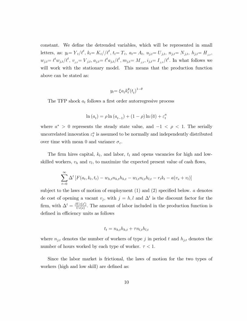
will work with the stationary model. This means that the production function

above can be stated as:

yt= �atk�t (tt)

1��

The TFP shock at follows a �rst order autorregresive process

ln (at) = � ln (at�1) + (1� �) ln (a) + "at

where a� > 0 represents the steady state value, and �1 < � < 1: The serially

uncorrelated innovation "at is assumed to be normally and independently distributed

over time with mean 0 and variance �":

The �rm hires capital, kt; and labor, tt and opens vacancies for high and low-

skilled workers, vh and vl, to maximize the expected present value of cash �ows,

1Xt=0

�t [F (at; kt; tt)� wh;tnh;thh;t � wl;tnl;thl;t � rtkt � a(vs + vl)]

subject to the laws of motion of employment (1) and (2) speci�ed below. a denotes

de cost of opening a vacant vj; with j = h; l and �t is the discount factor for the

�rm, with �t = �Uc(s0)Uc(s)

: The amount of labor included in the production function is

de�ned in e¢ ciency units as follows

tt = nh;thh;t + �nl;thl;t

where nj;t denotes the number of workers of type j in period t and hj;t denotes the

number of hours worked by each type of worker. � < 1:

Since the labor market is frictional, the laws of motion for the two types of

workers (high and low skill) are de�ned as:

10

nh;t+1 = nh;t(1� �s) + qh;tvh;t + �nl;t (1)

nl;t+1 = nl;t(1� �l) + ql;tvl;t � �nl;t (2)

where qj;t represents the perceived probability that a vacancy of type j get matched

with an unemployed worker of the same type. �nl;t represents the fraction of low-

skilled unemployed workers that su¤er an upgrade of skills every period. This move-

ment occurs with exogenous probability �. Thus, upgrading follows a Poisson process

with � rate which is independent of other processes in the model.

The labor market - The labor market is modellized as a frictional market in

which �rms and workers engage in employment relationships. The total number of

matches per unit of time is represented by the following technology

mj;t = m(vj;t , uj;t)

where uj;t represents the total number of type j searchers and vj;t the total number

of vacancies of type j. This matching function is increasing in both arguments,

concave and homogeneous of degree one.

The job vacancies and the unemployed workers that are matched at any point

in time t, are randomly selected from the sets v and u: Therefore, the process that

changes the state of vacant jobs to �lled vacant is a Poisson with rate qj;t=mj;t

vj;t:

Similarly, unemployed workers move into employment with probability �j;t=mj;t

uj;t:

The empirical literature has further found that a log-linear Cobb-Douglas ap-

proximation of the matching function �ts the data well2. So, in our model, the total

number of matches at time t is given by a Cobb-Douglas matching function in the

total number of searchers and vacancies of type j.

2see Pissarides (1990), ch.1 and Petrongolo and Pissarides (2001) for a survey.

11

mj;t = �jv�jj;tu

1��jj;t

�j is called the "e¢ ciency parameter" of the matching function. Under the Cobb-

Douglas speci�cation above, the probability of �nding a job, �j increases with the

tightness ratio ( vu) with elasticity less 1� �j < 1:

Households and Preferences - The economy is populated by identical, in�nitely-

lived households. In each household there are high skilled and low skilled workers.

The measure of type j workers is denoted by ej, for j = h; l and the total measure

of workers is normalize to one. We assume a complete set of insurance markets such

that the worker�s saving choices do not depend on its state on the labor market.

Thus there is a representative household that solves the following problem:

Max E

( 1Xt=0

�tU(ct; ht)

)(3)

where ct denotes consumption and ht denotes time spent at the work place. The

speci�cation of the utility adopted in our model is the following:

U(ct; ht) = log (ct) + nh;t�nht +nl;t�

nlt +uh;t�

uht +ul;t�

nlt

where �nit = �1i(1�hi;t)1��

u

1��u and �uit = �2i(1�et)1��

u

1��u . This function, is the one used

in Andolfatto (1996). Although is not the standard speci�cation in RBC models,

it would allow us to analyze straightforward the implications of introducing the

assumption of loss of skills during unemployment with respect to the "reference

model" in the literature.

The household has to decide how to split current income between consumption

and investment. Its income is made up of capital income, unemployment bene�ts

and the wage bill net of the lump sum, t, they have to pay to the government

to �nance the unemployment insurances, bj;t. Therefore, the household�s budget

constraint in period t is

12

ct+it+t � wh;tnh;thh;t+wl;tnl;thl;t+uh;tbh;t+ul;tbl;t+rtkt+pt

and investment is de�ned as follows:

it= `kt+1�(1� �)kt

Unemployment is a predetermined variable whose laws of motion are given by:

uh;t+1 = uh;t �mh;t + �hnh;t � uh;t

ul;t+1 = ul;t �ml;t + �lnl;t + uh;t

where uj;t denotes the measure of type j searchers, �j is the exogenous rate of

job destruction and �j is the perceived probability that an unemployed worker be

matched in period t: uh;t represents the fraction of workers that su¤er from a loss

of skill while unemployed. As we said, this process follows a Poisson distribution

with parameter : Like we have normalized our population to one, this means that

every period a fraction of the high skilled workers su¤er a "decapitalization" while

becoming long term unemployed.

Optimal contract - Following the standard literature on frictional unemploy-

ment, we assume that wages are the solution to a Nash-bargaining problem. Hence,

if we denote as pj the worker�s bargaining power, the optimal contract is given by

wj;thj;t=argmaxnW pnj;tJ

(1�p)nj;t

o; for j = h; l

where Wnj ;t and Jnj ;t represent the income value of employment of type j to the

household and the �rm respectively. pj will be treated as a constant parameter

strictly between 0 and 1:

The income value of high-skill employment to the household in units of the

consumption good is given by:

13

Wnh(Ht ) = �twh;thh;t+(�

n��u) + �Et�Wnh(

Ht+1)

�(1� �h��h)

+ ��E�Wnl(

Ht+1)

�� Et

�Wnh(

Ht+1)

��and is made up of three components: (i) the household gain in terms of wages be-

cause an additional high-skill agent starts working (ii) the loses in terms of leisure

that this new job generates and (iii) the expected present value of this job in the

future. This expected present value is formed by the continuation value of the job,

that is the net probability of keeping a high-skill employment, minus the probability

that the high-skill worker su¤er from a depreciation of his human capital and

become a low-skilled worker

The minimum wage the worker is going to accept comes fromWnh(Ht ) = 0: No-

tice that the high skilled worker takes into account the possibility of becoming long

term unemployed and with probability loosing some of his skills, therefore he is

willing to accept a lower wage than in the standard case in which = 0:

Similarly, the �rm�s marginal bene�t from employment is made up of the job�s

yields, i.e., the contribution to output of this marginal worker minus the returns to

his work, plus the expected present value of this job in the future.

Jnh(Ft ) = F nh;t�wh;thh;t+�Et

��t+1�tJns(

Ft+1)

�(1� �h)

For low-skill workers, the household�s marginal value of low skill employment is given

by the equation below, which includes the net gain in utility for an additional low

skill worker plus the expected present value of this job in the future.

Wnl(Ht ) = (�

n��u) + �twl;thl;t+�Et�Wnl(

Ht+1)

�(1� �l;t��l)

The �rms�marginal value of low skill employment equals the job�s yields plus

the expected present value of this position in the future.

14

Jnl(Ft ) = Fnl;t�wl;thl;t+�Et

��t+1�tJnl(

Ft+1)

�(1� �l)

+��Et

��t+1�t

�Jns(

Ft+1)� Jnl(Ft+1)

��notice that this expected present value includes the probability � of transforming

the low quality match into a high quality one. Jnh(Ft ) = 0; gives the maximum

compensation that the employer is willing to pay3.

From the �rst order condition of this maximization problem, we can know that

the worker will get a share pj of the total income generated by the match.

(1� pj)1

�tWnj ;t= pjJnj ;t

Therefore, the optimal contract for each type of worker in this economy is given by

the reservation wage and a fraction p of the net surplus they create by accepting the

job o¤er. Net surplus means the product value net of what workers give up in terms

of leisure and reservation wage. These optimal contracts can expressed as follows:

wh;thh;t = phFnh;t+phahvh;tuh;t

+ph

�ahqh;t

� alql;t

�+(1� ph)bh;t

�(1� ph)ct��1;h

(1� hh;t)(1��h)(1� �h)

� �2;h(1� e)(1��h)(1� �h)

�The reservation wage of a high-skilled worker is given by the unemployment in-

surance plus the leisure in terms of utility enjoyed by the potential worker. The

net surplus is given by the contribution of the worker to the output, which is his

marginal productivity plus the savings in terms of posting vacancies�cost and the

opportunity cost for the �rm of not hiring the high skilled worker given that with

3Note that if the �rm o¤ers this maximum compensation to the worker, it would generate

negative pro�ts in the steady state, because it does not take into account the fact that posting

vacancies is a costly activity.

15

probability he can su¤er a depreciation of skills net of what the worker gives up

which is his reservation wage.

Similarly, the optimal contract for the low-skill worker is given by the following

equation:

wl;thl;t = plFnl;t+plalvl;tul;t+pl�

�ahqh;t

� alql;t

�+(1� pl)bl;t

�(1� pl)ct��1;l(1� hl;t)(1��l)(1� �l)

� �2;h(1� e)(1��h)(1� �h)

�The only di¤erence with respect to the optimal contract for the other type of workers

is that now, the �rms takes into account that when it hires a low-skill worker he can

become high-skill type with probability �:

To disentangle wages and hours worked we need two additional equations. We

can compute the optimal number of hours for each type of worker di¤erentiating

the total surplus of each type of match Sj;t= 1�tWnj ;t+Jnj ;t with respect to the hours

@Sj;t@hj;t

; so that the optimal number of hours worked for each type of worker can be

represented as:

�11

�t(1� hj;t)

(��j)= (1� �)ytlt

De�nition of the recursive equilibrium - We can de�ne the equilibrium of

this economy as a set of in�nite sequences for the rental price of capital frtg, wagerates fwh;t; wl;tg, employment and unemployment levels fnh;t; nl;t; uh;t; ul;tg, capitalfktg, consumption fctg; vacancies fvh;t; vl;tg, hazard rates for workers f�h;t; �l;tg andvacancies fqs;t; ql;tg, such that,(i) Taking the rental prices and matching rates as given, fktg, fnh;t; nl;tg and

fvh;t; vl;tg maximize the �rms�pro�ts(ii) Wages are the solution to the Nash bargaining problem

(iii) Taking wages, the rental price of capital and hazard rates, fctg and fktgsolves the household optimization problem

(iv) Hazard rates are given by the matching function

16

4 Estimation of the model

The model presented above has a large number of parameters. This rises the problem

of assigning values to all of them. Standard calibration does not seem the best

technique when the models are richly parameterized given that neither the focus on

a limited set of moments of the model nor the transfer of microeconomics estimates

from one model to another will provide the discipline to quantify the behavior of the

model; so we have to rely in alternative methods that allow us to properly estimate

the parameters of the model. We will estimate the parameters of our model via

Maximum Likelihood.

Maximum Likelihood provides a systematic procedure to give values to all the

parameters of interest. This means that we have to evaluate the likelihood function

of our DSGE model. Except in a few cases, there is no analytical or numerical

procedure to directly do it. But we can transform the theoretical model into a state-

space econometric model and under the assumptions that the shocks to the economy

are normally distributed and the linear approximations of the policy functions of the

model, we can look for a numerical approximation of the likelihood function with

the help of the Kalman �lter. In what follows we explain this in more detail.

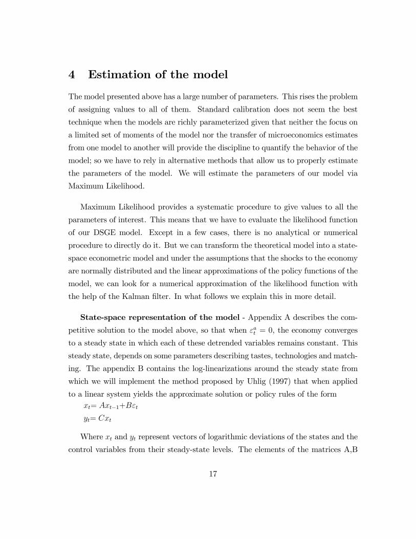
State-space representation of the model - Appendix A describes the com-

petitive solution to the model above, so that when "at = 0, the economy converges

to a steady state in which each of these detrended variables remains constant. This

steady state, depends on some parameters describing tastes, technologies and match-

ing. The appendix B contains the log-linearizations around the steady state from

which we will implement the method proposed by Uhlig (1997) that when applied

to a linear system yields the approximate solution or policy rules of the formxt= Axt�1+B"t

yt= Cxt

Where xt and yt represent vectors of logarithmic deviations of the states and the

control variables from their steady-state levels. The elements of the matrices A,B

17

and C depend on some of the model structural parameters.

The solution above considers that there is only one shock, the technology shock,

driving the business cycle. This makes the model stochastically singular, i.e., the

model predicts that certain combinations of the endogenous variables will hold with

equality, and if in the data these exact relationships do not hold, maximum likelihood

estimation will not be a valid method for the estimation.

Therefore, we should do any transformation in the model that allow us to over-

come this problem. As Ireland (2004) explains, there are two common approaches

to face the stochastic singularity problem. The �rst one consists in increasing the

number of shocks in the model until we have the same number of shocks as number

of time series used in the estimation; whereas the second approach, which is the

one we use here, consists in augmenting last equation of the system above with an

error term or measurement error, met. These errors represent the movements in the

data that the theory does not explain (those movements that are not generated by

the TFP shock, in our case) and are uncorrelated across variables. Then we have a

system of the form:st= Fst�1+V "t

ft= Gst+met

where ft denotes a vector of variables observed at date t, and st is the state vector,

F and G are again matrices of parameters. The �rst equation of the system is

known as the state equation and the second is known as the observation equation.

Vectors "t and met are white noise vectors with E["t"0t] = Q and E[metme

0t] = R:

Also E["tme0t] = 0

The advantage of this approach with respect to the �rst one, in which we have

to include additional shocks relies on the fact that no restrictions are imposed.

Otherwise, as Ireland (2004) says "it would have required to lean even harder in

18

economic theory by making further and speci�c assumptions about the behavior of

the economy".

Thus, once we have included this measurement errors, our theoretical DSGE

model takes the form of a state-space econometric model whose parameters can now

be estimated via maximum likelihood4.

Kalman �lter and approximation of the likelihood function - The em-

pirical model written as a state-space econometric model, allows for the evaluation

of the likelihood function using the Kalman �lter algorithm explained in detail in

Hamilton (1994, Chapter 13).

The ultimate objective is to estimate the values of the unknown parameters

in the system on the basis of these observations f1; f2; :::; fT . The Kalman �lter

works as a recursive estimator that takes initial values for the state-vector bstjt�1and its associate mean squared error Ptjt�1;to calculate linear least square forecast

of the state-vector for subsequent periods t=2,3,... T. This forecasts are of the

form. bstjt�1= bE[st+1j f t]:; where bE[st+1j f t] is the linear projection of st+1 on ft anda constant. The Kalman �lter has two main phases: prediction and update.

In the prediction phase, using the law of iterated projections, it plugs the forecastbstjt�1 into the observable equation to yield a forecasting of ftbftjt�1= Gbstjt�1

the error of this forecast is de�ned as wt= f t�dftjt�1 = Gst+met�Gbstjt�1�met withMSE E[(f t�dftjt�1)(f t�dftjt�1)0] = FP tjt�1F 0+R:In the second phase, the inference about the current value of st is updated on the

basis of the observation of ft to produce bstjt:: Introducing it into the state equationproduces a forecast of bst+1jt

4Ireland (2004) calls it "hybrid model" because it combines the power of the DSGE models with

the �exibility of a VAR.

19

bst+1jt = Fbstjt + 0evaluating bstjt by using the formula of updating a linear projection, and substitutingit above, we get the best forecast of st+1 based on a constant and a linear function

of the observable vector ft

bst+1jt = Fbstjt�1 +Kt(ft � bftjt�1)where Kt is the optimal Kalman gain matrix, which depends on the matrices F, G,

R and the stationary variance �t. Those matrices are not function of the data but

entirely determined by the population parameters of the process. bst+1jt denotes thebest forecast of st+1 based on a constant and a linear function of the observables ftif and only if Kt is the optimal gain matrix.

The application of the Kalman �lter let us calculate the log-likelihood function

of the hybrid model as

ln(L) = �3T2ln (2�)�1

2

TXt=1

ln jG�tG0j �1

2

TXt=1

w0t (G�tG0)�1wt

Using a numerical search algorithm one can �nd the set of parameters contained

in the matrices F, G, Q and R that maximize the likelihood function. Usually,

maximum likelihood estimations of this type are criticized because it is very di¢ cult

to be sure whether we are in the global maximum or on the contrary we are just in

a local one, given that the likelihood function displays a quite sinuous pattern. To

avoid this criticism with our estimations we borrow from physics another algorithm

called "simulated annealing" . This is a generic probabilistic meta-algorithm for

the global optimization problem, i.e. it looks for a good approximation to the

global optimum of a function in a large search space. Each step of the simulated

annealing algorithm replaces the current solution by a random "nearby" solution.

The allowance for these movements saves the method from becoming stuck at a local

minimum.

20

In principle, this numerical algorithm is allowed to select values of the parameters

that lie anywhere between the positive and the negative in�nity. But to ensure

that our parameters satisfy the theoretical restrictions listed in section 2, additional

constraints have been imposed5.

The data - Data is taken from the Federal Reserve Bank of St. Louis�FRED

database. Data for gross domestic income and wages is taken from the Bureau of

Economic Analysis. In the appendix C, we present detailed information about each

series. Monthly data has been transformed into quarterly data using averages. The

period selected goes from 1964-1 to 2005-4.

When the model takes the form of a state-space representation, it can be esti-

mated via maximum likelihood once analogs to the model�s variables are found in

the data. Therefore, Ct is de�ned as real personal consumption on non durables and

services plus government expenditure. Investment, It is de�ned as the sum of con-

sumption on durable goods plus investment. Vacancies, Vt are proxied by a widely

used index which re�ects the number of "help-wanted" advertisement registered in

US newspapers. Nt comes directly from the number of civilian employment, and

thus unemployment can be computed as 1�N t.

All the variables have been divided by the civilian population aged 16 or over,

so as to have them in per capita terms. On top of that we have taken logarithms

of all the variables and calculated the growth rates when necessary. Series have not

been �ltered in any other way.

Finally, to make them comparable with the vectors of logarithmic deviations of

the variables from their steady-state levels, we have to use the de�nitions:

5In particular, some of ours parameters are constrained to be positive, so we constraint the

algorithm to work with absolute values. Many of ours parameters are probabilities that should lie

between zero and one, so we again constraint the algorithm to work with the logistic transformation

of the parameter.

21

bct= log (ct)� log (c)bit= log (it)� log (i)Pr odt= log ( Pr odt)� log (Pr od)� t log (`)

btt= log (tt)� log (t)b�t= log (�t)� log (�)

for all t=1....T. Remember that to solve the problem we have normalized out-

put to 1. Therefore, consumption and investment here are de�ned as bct = d� cd;tyt

�.

and bit = d� id;tyt

�. Productivity is growing at rate ` in steady state. Once those

transformations are made, the vector of observable is given by:

ft=h bct bit btt dPdt b�t i

Parameter estimates - Usually algorithms for computing maximum likelihood

estimates have the drawback that they do not produce standard errors. This means

that we should look numerical approximations of the derivatives of the likelihood

function so as to compute the information matrix and then the standard errors.

Fortunately, we know that if certain regularity conditions hold6, the maximum

likelihood estimates are consistent and asymptotically normal. Under these circum-

stances, the information matrix for a sample of size T can be calculated from the

second derivatives of the maximized log-likelihood function as

6These conditions include that the model must be identi�ed, the eigenvalues of A are inside

the unit circle, the true values of the estimations do not fall on a boundary of the allowable

parameter space and that variables xt behave asymptotically like a full-rank linearly indeterministic

covariance-stationary process

22

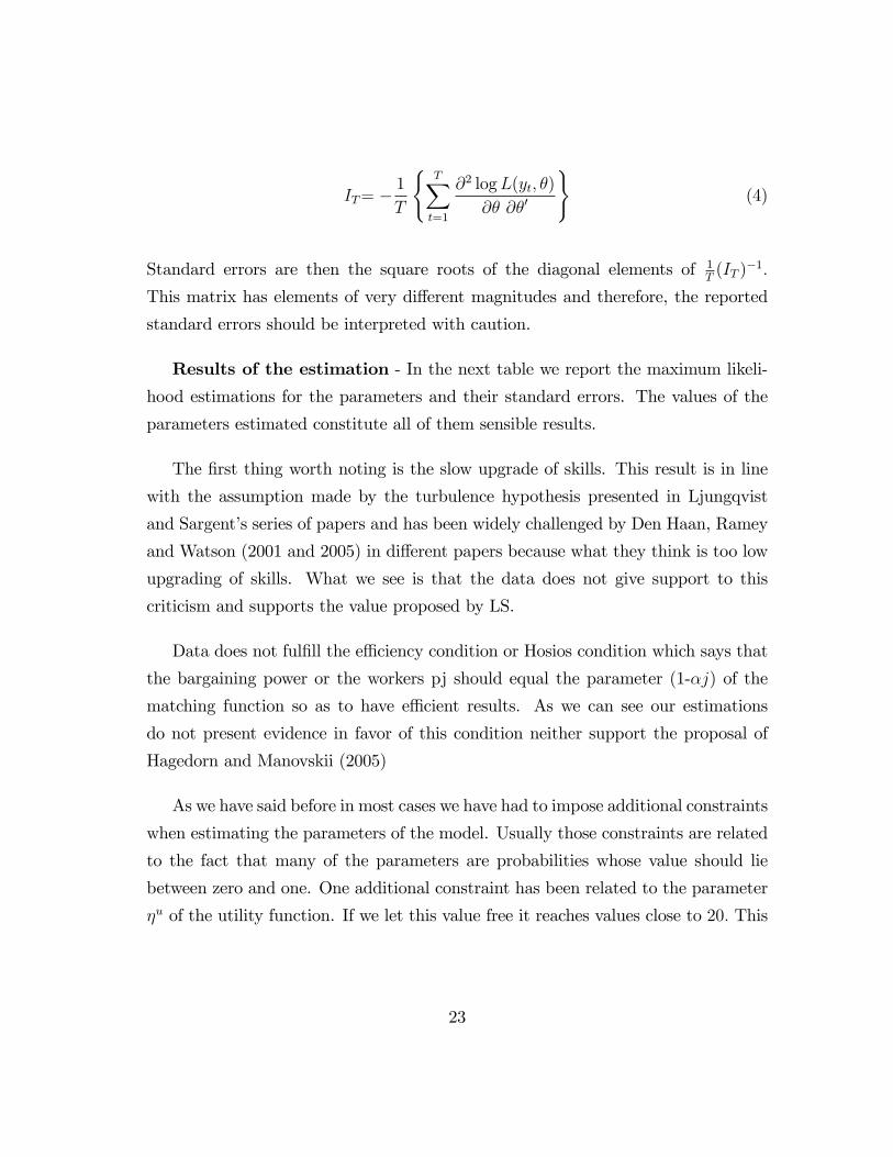
IT= �1

T

(TXt=1

@2 logL(yt; �)

@� @�0

)(4)

Standard errors are then the square roots of the diagonal elements of 1T(IT )

�1:

This matrix has elements of very di¤erent magnitudes and therefore, the reported

standard errors should be interpreted with caution.

Results of the estimation - In the next table we report the maximum likeli-

hood estimations for the parameters and their standard errors. The values of the

parameters estimated constitute all of them sensible results.

The �rst thing worth noting is the slow upgrade of skills. This result is in line

with the assumption made by the turbulence hypothesis presented in Ljungqvist

and Sargent�s series of papers and has been widely challenged by Den Haan, Ramey

and Watson (2001 and 2005) in di¤erent papers because what they think is too low

upgrading of skills. What we see is that the data does not give support to this

criticism and supports the value proposed by LS.

Data does not ful�ll the e¢ ciency condition or Hosios condition which says that

the bargaining power or the workers pj should equal the parameter (1-�j) of the

matching function so as to have e¢ cient results. As we can see our estimations

do not present evidence in favor of this condition neither support the proposal of

Hagedorn and Manovskii (2005)

As we have said before in most cases we have had to impose additional constraints

when estimating the parameters of the model. Usually those constraints are related

to the fact that many of the parameters are probabilities whose value should lie

between zero and one. One additional constraint has been related to the parameter

�u of the utility function. If we let this value free it reaches values close to 20: This

23

value seems extremely large and we have constrained it to lie between 0 and 5.

Table 2: Estimated parameters and standard deviations

Parameter Value Explanation Std. error

�h 0:80 elasticity vacancies type h 0:0010

�l 0:80 elasticity vacancies type l 0:0021

� 0:01 upgrade of skills 0:0040

� 0:95 technology persistence 0:0119

" 0:01 variance 0:0001

ph 0:10 bargaining power workers 0:0009

pl 0:355 bargaining power workers 0:0007

g 1:005 deterministic growth rate 0:0001

� 0:583 elasticity of capital 0:0027

� 0:03 depreciation of capital 0:0059

� 0:90 e¢ ciency units of low product workers 0:0124

�h 0:0781 exog. destruc rate for h 0:0027

�l 0:0897 exog. destruc rate for l 0:0020

�u 3:3341 parameter utility function 0:0009

The deterministic growth rate of the economy takes a value close to one. This

means that we can perfectly work with a stationary model. The less satisfactory

results are for the values driving the investment and capital accumulation of the

economy. We obtain a value of � close to 0.6 whereas the standard value in the

literature is close around 0.4. Also the depreciation of capital, �; takes a higher

value than what is standard. This has led us to estimate a second version of the

model, in which we have constrained the values of those parameters to take the

standard values. The performance of variables such as consumption and investment

improves with this new speci�cation as we will see afterwards.

It is also quite common to obtain low estimates for the discount factor �, showing

the preference of the household for consumption today. What we have done is to

estimate the parameters of the model keeping � �xed and equal to 0.99.

24

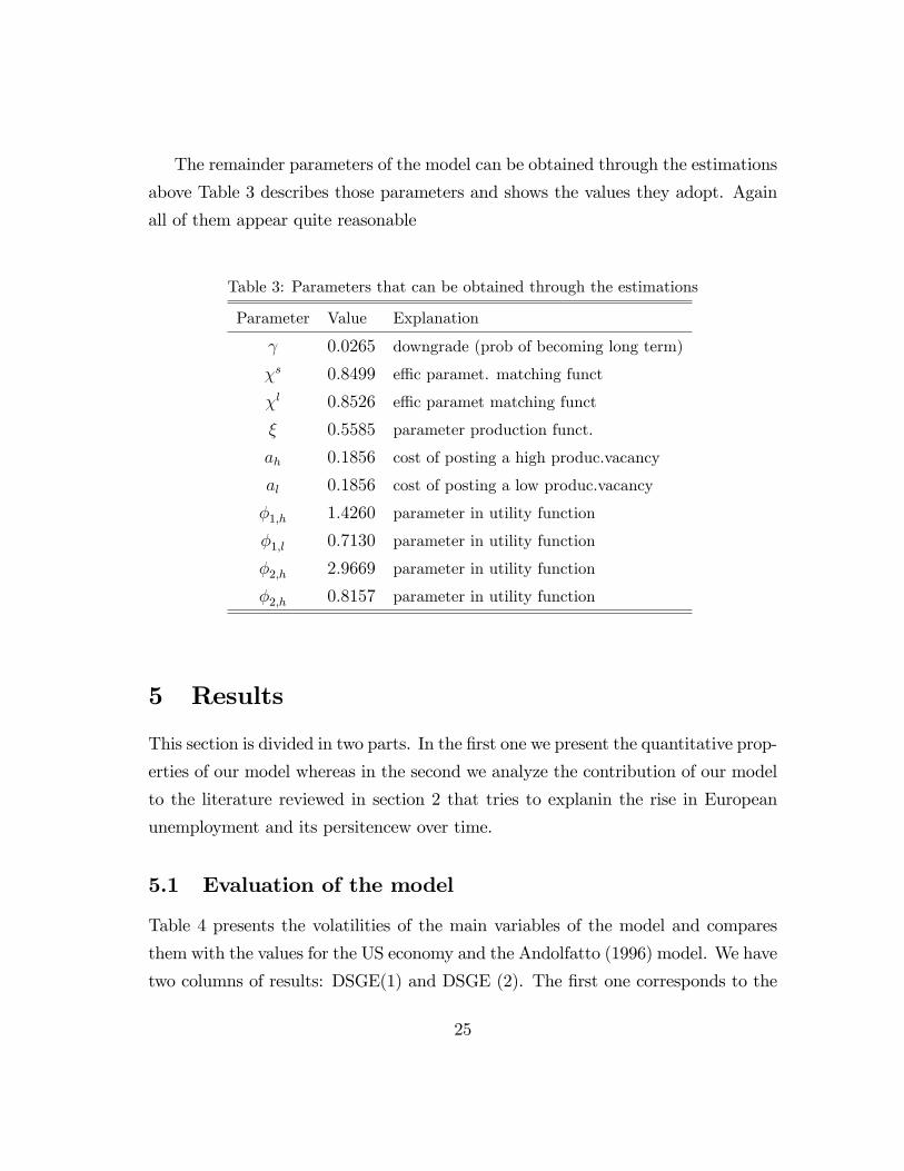
The remainder parameters of the model can be obtained through the estimations

above Table 3 describes those parameters and shows the values they adopt. Again

all of them appear quite reasonable

Table 3: Parameters that can be obtained through the estimations

Parameter Value Explanation

0:0265 downgrade (prob of becoming long term)

�s 0:8499 e¢ c paramet. matching funct

�l 0:8526 e¢ c paramet matching funct

� 0:5585 parameter production funct.

ah 0:1856 cost of posting a high produc.vacancy

al 0:1856 cost of posting a low produc.vacancy

�1;h 1:4260 parameter in utility function

�1;l 0:7130 parameter in utility function

�2;h 2:9669 parameter in utility function

�2;h 0:8157 parameter in utility function

5 Results

This section is divided in two parts. In the �rst one we present the quantitative prop-

erties of our model whereas in the second we analyze the contribution of our model

to the literature reviewed in section 2 that tries to explanin the rise in European

unemployment and its persitencew over time.

5.1 Evaluation of the model

Table 4 presents the volatilities of the main variables of the model and compares

them with the values for the US economy and the Andolfatto (1996) model. We have

two columns of results: DSGE(1) and DSGE (2). The �rst one corresponds to the

25

values of the parameters presented in Table 3 above whereas DSGE(2) represents

the more constrained model explained above. In particular, we have proceed again

with the estimation of the main parameters of the model but keeping the values of

�; � and � �xed.

What we can see from these values is that the volatility of total hours worked,

employment, hours per worker and tightness increase substantially with respect to

the Andolfatto model. Our model increase also the volatility of both unemployment

and vacancies with respect to the search economy or the Andolfatto results. We can

see this as a success given the large literature dealing with it nowadays.

The model has some di¢ culty in explaining the larger volatility of the variable

hours per worker, which results substantially larger in the model than in the data.

Accordingly, the volatilities of the wage bill and the labor share of output also

result more volatile than in the data. This result depends to a great extent on the

parameter �u of the utility function that we have not allow to take larger values than

5. Probably, a more standard speci�cation of the utility function could yield more

satisfactory results concerning the performance of this variable or even allowing for

this parameter to take larger values can partially solve the problem.

The DSGE(2) yields overall better results in terms of volatilities than DSGE(1).

We do not see any inconvenient in dealing with these model instead with the less

restricted one. The performance of the investment, consumption and tightness im-

proves signi�cantly when allowing for those constraints while the remaining values

are pretty similar to those obtained under the DSGE(1).

26

Table 4: Volatilities

Variable US Economy RBC Search DSGE (1) DSGE (2)

Consumption 0:56 0:32 0:27 0:32

Investment 3:14 2:98 2:08 3:12

Total hours 0:93 0:59 0:80 0:75

Employment 0:67 0:51 0:72 0:70

HoursnWorker 0:34 0:22 1:06 1:07

Tightness 3:30 4:61 6:78

Wage bill 0:97 0:94 1:86 1:89

Labor share 0:68 0:10 1:17 1:00

Productivity 0:64 0:46 0:27 0:32

Real Wage 0:44 0:39 0:26 0:27

One of the major interests of the theoretical model presented in this paper is

that if satisfactory, it can be used to analyze European labor markets. One common

characteristic of those markets is the existence of long-term unemployment or, in

other words, high persistence of unemployment. The standard RBC model with

frictional labor markets, although satisfactory in replicating the persistence of US

unemployment, have major problems when replicating the persistence of European

labor markets (see Esteban-Pretel, 2004). When we introduce the assumption of

loss of skills during unemployment in combination with unemployment bene�ts,

the persistence of unemployment increases substantially. For example, under the

reference Andolfatto model, 86 per cent of the unemployed workers that lose their

jobs remain unemployed one quarter apart whereas only 18 per cent of them remain

unemployed within a year. Under our speci�cation almost half of them remain

unemployed within a year, which constitutes almost 70 per cent of the unemployed

27

workers who have su¤ered from a depreciation of skills.

Table 5: Persistence of unemployment

Variable (x) x(t) x(t+ 1) x(t+ 2) x(t+ 3) x(t+ 4)

Search Economy

Total unemployment 1 0:86 0:63 0:39 0:18

Turbulent workers � � � � �DSGE (1)

Total unemployment 1 0:93 0:80 0:63 0:45

Turbulent workers 1 0:98 0:91 0:80 0:67

DSGE (2)

Total unemployment 1 0:94 0:80 0:63 0:45

Turbulent workers 1 0:98 0:91 0:80 0:67

5.2 Implications for the labor market performance

As we have seen at the begining of this paper, the turbulence hypothesis relies

on the combination of microeconomic shocks to the human capital of unemployed

workers and labor market institutions to explain the steadily increase in unemploy-

ment in Europe from the late 1970s onwards. In particular, Ljungqvist and Sargent

(1998) central assumption is that "the last couple of decades saw an increased prob-

ability of human capital loss at the time of an involuntary job displacement". This

increase in the probability of losing skills in combination with generous unemploy-

ment bene�ts, produce high long-term unemployment.

Given that the values of the estimated parameters are in line with the values

proposed by LS, we can split the initial sample into two sub-samples and analyze

whether the data gives support to the hypothesis of an increase in turbulence or

not. Therefore, we split the sample into two disjoint sub-samples. The �rst one

28

covers the period 1964Q1-1980Q1, and the second runs the rest of the sample, i.e.

1980Q2-2005Q1. The breakpoint corresponds to the date around which we consider

the European unemployment started rising7.

Then we re-estimate the parameters and check for their stability. Across the

board, the test reject the null hypothesis of parameter stability. This result is in

line with previous �ndings of Ireland (2004) and Altug (1989) and Stock and Watson

(1996) who also found evidence of instability in parameters in RBC and VAR models

respectively.

But what is more interesting for our analysis, is that the parameter that

measures the probability of human capital loss remains constant along the two sub-

samples and for both speci�cations of the model - without and with constraints on

some of the parameters-.

Period Parameter

t1= 1964Q1� 1980Q1 1=0:0265

t2= 1980Q2� 2005Q4 2=0:0265

Conclusion 1= 2

We see this result very interesting as far as it contributes to the literature on

unemployment in the following way: According to our model and the estimation of

its parameters, we do not observe evidence in favor of an increase in the probability

of human capital loss. This does not mean that we �nd the LS explanation wrong

because, in spite of the fact that we do not observe an increase in the value of this

parameter, the turbulence hypothesis is necessary to improve the performance of

the RBC model and, more important for the understanding of unemployment, it

is able to increase the persistent unemployment and consequently generate long-

term unemployment. This is a characteristic that previous RBC models embedding

matching models in the labor market were unable to produce.7We have tried di¤erent breakpoints running from 1975Q4 to 1982Q4, giving all of them similar

results.

29

Stated in other words, we explain the increase in unemployment in the following

terms: We belive that there is a negative aggregate shock that increases the pool

of unemployed workers. This makes the fraction of turbulent workers increase- not

because the probability of losing skills increases but because the initial pool has

become bigger due to an aggregate shock-. At this point we have an increase in

the number of turbulent unemployed workers who have loss their initial skills but

receive unemployment bene�ts that correspond to the high skill level. The rest of

the story is the LS one.

In a way, our results conciliate the macro and micro explanations proposed in

the literature to explain the increase in unemployment and its persistence over time.

6 Conclusion

In this paper we have proposed a DSGE model in which the labor market is explic-

itly modellized as a frictional market where �rms and workers engage in productive

job matches. We have also introduced the assumption of loss of skills during un-

employment to analyze the hypothesis of turbulence proposed in the literature to

explain the steadily increase in the European unemployment since the late 1970s.

We have then brought the model to the data. We have estimated the parameters

of the model via maximum likelihood and we have seen that the values obtained

are in line with those proposed by LS. In particular, we �nd very low probability of

upgrading skills for the already matched workers and similar value for the turbulence

parameter. We have also analyzed the quantitative properties of our model and we

have studied the stability of the probability of su¤ering from a depreciation of human

capital.

We �nd that the data does not give evidence of an increase of the probability

of losing skills once the match have been dissolved, contrary to the central assump-

tion of LS�s explanation. Nevertheless, allowing for this depreciation of the human

30

capital, generates long-term unemployment or a very strong persistence of the un-

employment for all workers in the economy and mainly for those who have su¤ered

the loss of skills.

Wrapping up, we conclude that according to our model we cannot accept the as-

sumption that an increase in the turbulence occurred at the end of the 70s. Instead

we �nd evidence on the existence of a negative aggregate shock that increased the

pool of unemployed workers. We do not see this as a rejection of subsequent expla-

nation given by LS, i.e. that we need the combination of the loss of skills assumption

and generous unemployment bene�ts to produce long-term unemployment and be

able to explain the steadily increase in unemployment over time.

In a way, our model conciliates the two streams of the literature that have tried to

explain the European unemployment dilemma based on the one hand on the combi-

nation of macroeconomic shocks and labor market institutions and the combination

of micro shocks and those labor market institutions, on the other hand.

31

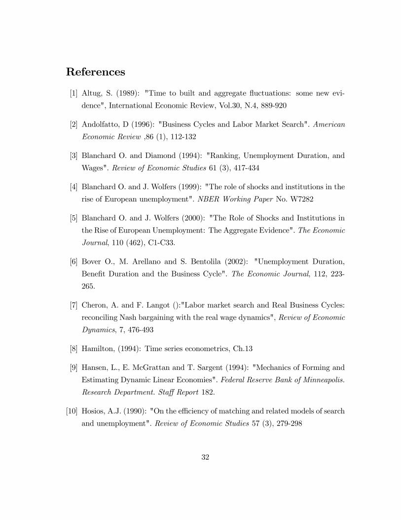
References

[1] Altug, S. (1989): "Time to built and aggregate �uctuations: some new evi-

dence", International Economic Review, Vol.30, N.4, 889-920

[2] Andolfatto, D (1996): "Business Cycles and Labor Market Search". American

Economic Review ,86 (1), 112-132

[3] Blanchard O. and Diamond (1994): "Ranking, Unemployment Duration, and

Wages". Review of Economic Studies 61 (3), 417-434

[4] Blanchard O. and J. Wolfers (1999): "The role of shocks and institutions in the

rise of European unemployment". NBER Working Paper No. W7282

[5] Blanchard O. and J. Wolfers (2000): "The Role of Shocks and Institutions in

the Rise of European Unemployment: The Aggregate Evidence". The Economic

Journal, 110 (462), C1-C33.

[6] Bover O., M. Arellano and S. Bentolila (2002): "Unemployment Duration,

Bene�t Duration and the Business Cycle". The Economic Journal, 112, 223-

265.

[7] Cheron, A. and F. Langot ():"Labor market search and Real Business Cycles:

reconciling Nash bargaining with the real wage dynamics", Review of Economic

Dynamics, 7, 476-493

[8] Hamilton, (1994): Time series econometrics, Ch.13

[9] Hansen, L., E. McGrattan and T. Sargent (1994): "Mechanics of Forming and

Estimating Dynamic Linear Economies". Federal Reserve Bank of Minneapolis.

Research Department. Sta¤ Report 182.

[10] Hosios, A.J. (1990): "On the e¢ ciency of matching and related models of search

and unemployment". Review of Economic Studies 57 (3), 279-298

32

[11] Ireland, P. (2004): "A method for taking models to the data". Journal of Eco-

nomic Dynamics and Control, 28,1205-1226

[12] Jackman, R and R. Layard (1991): "Does long-term Unemployment Reduce a

Person�s Chance of a Job? A Time Series Test", Economica, 58 (229), 93-106

[13] Layard, R., S. Nickell and R. Jackman (1991): Unemployment, Macroeconomic

Performance and the Labour Market, Oxford, Oxford University Press.

[14] Ljungqvist, L. and T. Sargent (1998):"The European Unemployment

Dilemma", Journal of Political Economy, 106, 514-550.

[15] Ljungqvist, L. and T. Sargent (2002): "The European Employment Experi-

ence", CEPR Discussion Paper No. 3543

[16] Ljungqvist, L. and T. Sargent (2004): " European Unemployment and Turbu-

lence revisited in a matching model", CEPR Discussion Paper No. 4183

[17] Ljungqvist, L. and T. Sargent (2005): " Jobs and Unemployment in Macroeco-

nomic Theory: A turbulence laboratory", CEPR Discussion Paper No. 5340

[18] Den Haan, W. G. Ramey and J.Watson (2000):�Job destruction and propaga-

tion of shocks�, American Economic Review, 90(3), 482-498

[19] Den Haan, W, C. Haefke and G. Ramey (2001): "Shocks and Institutions in a

Job Matching Model", NBER Working Papers, No. 8463.

[20] Den Haan, W, C. Haefke and G. Ramey (2005): "Turbulence and unemploy-

ment in a job matching model", NBER Working Papers, No. 8463.

[21] Merz, M (1995):"Search in the labor market and the real business cycle", Jour-

nal of Monetary Economics, 36, 269-300.

[22] Nickel, S. (1979),"Estimating the probability of leaving unemployment" Econo-

metrica 4(5), 1249-1266

33

[23] Petrongolo, B. and C. Pissarides (2001): "Looking into the Black Box: A survey

of the matching function". Journal of Economic Literature 39, 390-431.

[24] Phelps, E. (1994): Structural Slumps. The modern equilibrium theory of unem-

ployment, interest and assets. Cambridge MA. Harvard University Press.

[25] Pissarides, C. (1992): "Loss of skill during unemployment and the persistence

of employment shocks", Quarterly Journal of Economics, 107(4),1371-1391

[26] Pissarides, C. (2000): Equilibrium Unemployment Theory. The MIT Press,

Cambridge. Second Edition

[27] Prescott, E. (2004): Why do Americans work so much more than Europeans?".

Federal Reserve Bank of Minneapolis Quarterly Review, 28 (1), 2-13.

[28] Rebelo, S (2005): "Real Business Cycle Models: Past, Present and Future",

mimeo

[29] Ravn, M (2005): "Labor Market Matching, Labor Market Participation and

Aggregate Business Cycles: Theory and Structural Evidence for the US", Eu-

ropean University Institute, mimeo

[30] Ravn, M (2006): "The Consumption-Tightness Puzzle", European University

Institute, mimeo

[31] Ruge-Murcia, F. (2003): "Methods to Estimate Dynamic Stochastic General

Equilibrium Models", Université de Montréal, cahier 2003-23.

[32] Shimer, R (2005): "The Cyclical Behaviour of Equilibrium Unemployment and

Vacancies", American Economic Review 95(1), 25-49

[33] Uhlig, H. (1997): "A toolkit for Analyzing Nonlinear Dynamic Stochastic Mod-

els Easily"

34

A Appendix: solving for the non-stochastic equi-

librium

A.1 Households

The household maximizes the following problem

W (Ht ) =maxc;k0

(log (ct) + nh;t�1;h

(1�hh;t)(1��h)

(1��h)+uh;t�2;h

(1�e)(1��h)(1��h)

+nl;t�1;l(1�hl;t)

(1��l)

(1��l)+ul;t�2;l

(1�e)(1��l)(1��l)

+�EtW (Ht+1)

)

subject to the budget constraint and the law of motion for capital

ct+it+�t= wh;tnh;thh;t+wl;tnl;thl;t+uh;tbh;t+ul;tbl;t+rtkt+�t

kt+1= (1� �)kt+it

where ul;t= ut;t+ub;t and bl;t=ut;tbh;t+ub;tbb;t

ul;t

The �rst order conditions of the problem and the envelope theorem are presented

below:

w.r.t. consumption 1ct= �t

w.r.t. capital t+1 �Et�Wk(

Ht+1)

�= �t

budget constraint ct+kt+1�(1� �)kt = wh;tnh;thh;t+wl;tnl;thl;t+uh;tbh;t+ul;tbl;t+rtkt+�t

envelope theorem Wk(Ht ) = �t [(1� �) + rt]

35

and yield the optimal behavior of the household. Therefore, the optimal decisions

for the households are fully summarized by the following equations:

1 = �Et

n�t+1�t((1� �) + rt+1)

oct+it+�t= wh;tnh;thh;t+wl;tnl;thl;t+uh;tbh;t+ul;tbl;t+rtkt+�t

kt+1= (1� �)kt+it

A.2 Firms

The Bellman equation that represents the problem of the �rm can be stated as

follows:

J(Ft ) = maxk;n0h;n

0l;vh;vl

F (�atk�tL

(1��)t �wh;tnh;thh;t�wl;tnl;thl;t�rtkt�ahvh;t�alvl;t+�Eh�t+1

�tJ(Ft+1)

isubject to the laws of motion for employment and the AR process de�ning the

technology

nh;t+1= nh;t(1� �h) + qh;tvh;t+�nl;t

nl;t+1= nl;t(1� �l) + ql;tvl;t��nl;t

log at+1= � log at+(1� �) log a+"at+1

The �rst order conditions of the problem are presented below:

36

w.r.t capital (1� �) ytkt= rt

w.r.t vacancies for high-skill workers ah= �h;t qh;t

w.r.t vacancies for low-skill workers al= �l;t ql;t

w.r.t high-skill employment t+1 �h;t= �Et

h�t+1�tJnh(

Ft+1)

iw.r.t low-skill employment t+1 �l;t= �Et

h�t+1�tJnl(

Ft+1)

ilaw of motion for high-skill employment nh;t+1= nh;t(1� �h) + qh;tvh;t+�nl;t

law of motion for high-skill employment nl;t+1= nl;t(1� �l) + ql;tvl;t��nl;t

And applying the envelope theorem we have:

for high-skill employment Jnh(Ft ) = F nh;t�wh;thh;t+�h;t(1� �h)

for low-skill employment Jnl(Ft ) = F nl;t�wl;thl;t+�l;t(1� �l) + �(�h;t��l;t)

Thus, optimal decisions for the �rms are fully summarized by:

37

(1� �) ytkt= rt

ahqh;t= �Et

n�t+1�t

�Fnh;t+1 � wh;t+1hh;t+1 + ah

qh;t+1(1� �h)

�oalql;t= �Et

n�t+1�t

�Fnl;t+1 � wl;t+1hl;t+1 + al

ql;t+1(1� �l) + �

�ah

qh;t+1� al

ql;t+1

��onh;t+1= nh;t(1� �h) + qh;tvh;t+�nl;t

nl;t+1= nl;t(1� �l) + ql;tvl;t��nl;t

A.3 Matching

The standard speci�cation of the matching function is the following:

mj;t = �jv�jj;tu

1��jj;t

and the companion probabilities of matching for workers and vacancies are respec-

tively:

�j;t =mj;t

uj;tand qj;t =

mj;t

vj;t

A.4 Optimal contract:

To compute the optimal contract we just have to apply the �rst order condition of

the Nash bargaining problem, which can be stated as follows

(1� pj)1

�tWnj= pjJnj

38

The marginal value of high-skill and low-skill employment for the household comes

from the following expressions

Wnh(Ht ) =

(�1;h

(1�hh;t)(1��h)(1��h)

� �2;h(1�e)(1��h)(1��h)

+ �twh;tnh;thh;t � �tuh;tbh;t+�Et

�Wnh(

Ht+1)

�(1� �h � �h) + �

�E�Wnl(

Ht+1)

�� Et

�Wnh(

Ht+1)

�� )

Wnl(Ht ) =

(�1;l

(1�hl;t)(1��l)(1��l)

� �2;h(1�e)(1��h)(1��h)

+ �twl;thl;t � �tul;tbl;t+�Et

�Wnl(

Ht+1)

�(1� �l;t � �l)

)

which together with the income values of employment for the �rms, Jnh and Jnl,

yield the following contracts:

wh;thh;t=phFnh;t+phahvh;tuh;t

+ph

�ahqh;t

� alql;t

�+(1�ph)bh;t�(1�ph)ct

�1;h

(1�hh;t)(1��h)

(1��h)��2;h

(1�e)(1��h)(1��h)

!

wl;thl;t=plFnl;t+plalvl;tul;t

+pl�

�ahqh;t

� alql;t

�+(1�pl)bl;t�(1�pl)ct

�1;l

(1�hl;t)(1��l)

(1��l)��2;h

(1�e)(1��h)(1��h)

!

the optimal values for the hours worked of each type of worker are obtained via the

mutual surplus of the match

Sj;t=1

�tWnj ;t+Jnj ;t

and yield the following results

@Sh;t@hh;t

= ��1 1�t (1� hh;t)(��h)+(1� �) Yt

Lt

�1� �nh;thh;t

Lt

�= 0

@Sl;t@hl;t

= ��1 1�t (1� hl;t)(��l)+(1� �) Yt

Lt��1� �� nl;thl;t

Lt

�= 0

39

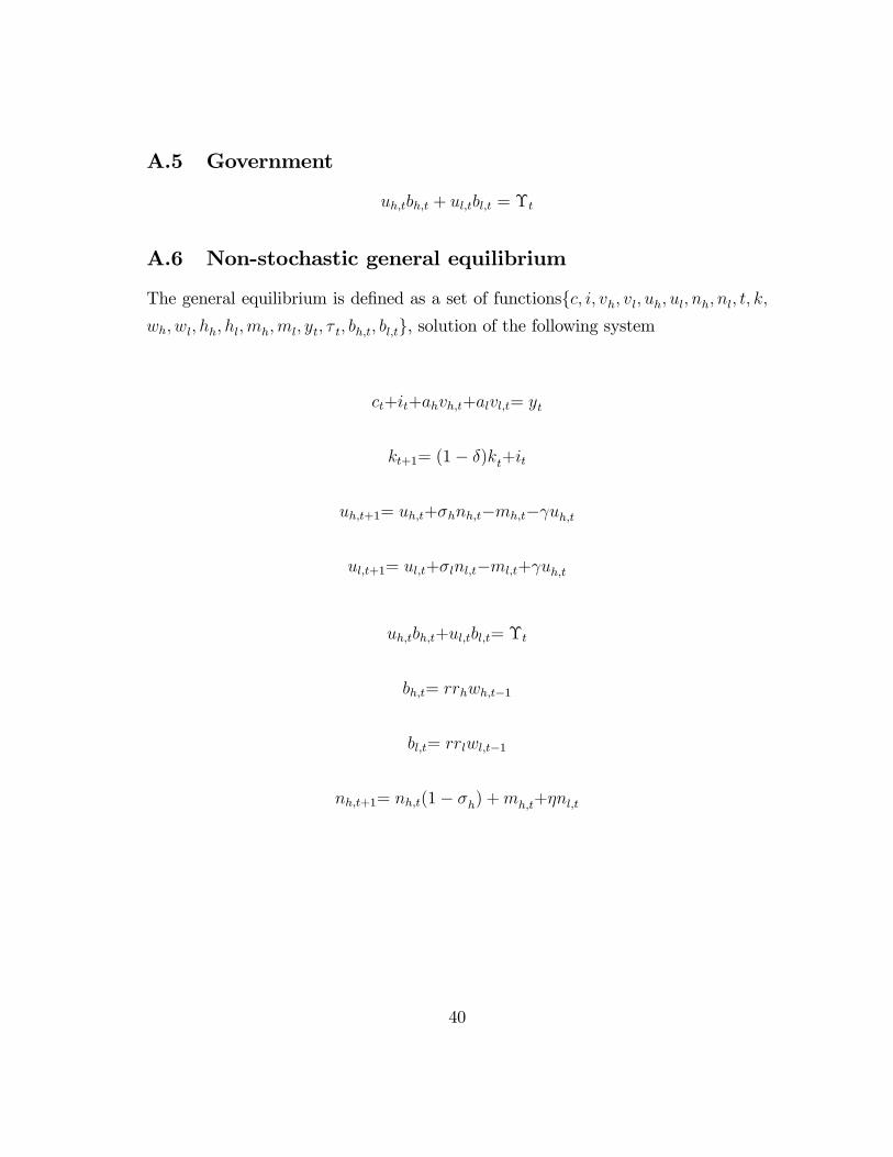
A.5 Government

uh;tbh;t + ul;tbl;t = �t

A.6 Non-stochastic general equilibrium

The general equilibrium is de�ned as a set of functionsfc; i; vh; vl; uh; ul; nh; nl; t; k;wh; wl; hh; hl;mh;ml; yt; � t; bh;t; bl;tg, solution of the following system

ct+it+ahvh;t+alvl;t= yt

kt+1= (1� �)kt+it

uh;t+1= uh;t+�hnh;t�mh;t� uh;t

ul;t+1= ul;t+�lnl;t�ml;t+ uh;t

uh;tbh;t+ul;tbl;t= �t

bh;t= rrhwh;t�1

bl;t= rrlwl;t�1

nh;t+1= nh;t(1� �h) +mh;t+�nl;t

40

nl;t+1= nl;t(1� �l) +ml;t��nl;t

yt= �Ak�(tt)

(1��)

tt= nh;thh;t+�nl;thl;t

mh;t= �hv�hh;tu

1��hh;t

ml;t= �lv�ll;tu

1��ll;t

wh;thh;t=phFnh;t+phahvh;tuh;t

+ph

�ahqh;t

� alql;t

�+(1�ph)bh;t�(1�ph)ct

�1;h

(1�hh;t)(1��h)

(1��h)��2;h

(1�e)(1��h)(1��h)

!

wl;thl;t=plFnl;t+plalvl;tul;t

+pl�

�ahqh;t

� alql;t

�+(1�pl)bl;t(1�pl)ct

�1;h

(1�hl;t)(1��l)

(1��l)��2;h

(1�e)(1��l)(1��l)

!

(1� �) ytLt

�1� �nh;thh;t

tt

�= ct�1(1� hh;t)

(��h)

(1� �) ytLt��1� �� nl;thl;t

tt

�= ct�1(1� hl;t)

(��l)

and the expectational equations

1 = �Et

nctct+1

�(1� �) + (1� �) yt+1

kt+1

�oahvh;tmh;t

= �Et

nctct+1

�Fnh;t+1 � wh;t+1hh;t+1 + ahvh;t+1

mh;t+1(1� �h)

�oalvl;tml;t

= �Et

nctct+1

�Fnl;t+1 � wl;t+1hl;t+1 + alvl;t+1

ml;t+1(1� �l) + �

�ahvh;t+1mh;t+1

� alvl;t+1ml;t+1

��o

41

Given that we also impose that 1 = nh;t + nl;t + uh;t + ul;t one of the laws of motion

above is a linear combination of the others plus the condition above and we have to

take this into account

B Log-linearized equations

B.1 Deterministic equations

0 = c�c(t) + i�i(t) + ahv�hvh(t) + alv

�l vl(t)� y

�y(t)

0 = k�k(t)� (1� �)k�k(t� 1)� i�i(t)

0 = n�l nl(t)� (1� �l��)n�l nl(t� 1)�m

�lml(t)

0 = n�hnh(t)� (1� �h)n�hnh(t� 1)�m

�hmh(t)� �n�l nl(t� 1)

0 = n�hnh(t) + n�l nl(t) + u

�huh(t) + u

�l ul(t)

0 = u�huh(t)� (1� )u�huh(t� 1)� �hn�hnh(t� 1) +m

�hmh(t)

y(t)� a(t)� �k(t� 1)� (1� �)l(t)) = 0

l�l(t) = n�hh�h[nh(t)hh(t)] + �n

�l h�l [nl(t)hl(t)]

mh(t)� �hvh(t)� (1� �h)uh(t) = 0

ml(t)� �lvl(t)� (1� �l)ul(t) = 0

42

0 = ph(1� �)y�

th�hh

� (y(t)� t(t)� hh(t)) + phahv�hu�h(vh(t)� uh(t� 1)) + (1� ph)b�hbh(t)

+ph ahv

�h

m�h

(vh(t)�mh(t))� ph alv

�l

m�l

(vl(t)�ml(t)) + (1� ph)�2;hc�(1� e)(1��h)(1� �h)

c(t)

�(1� ph)�1;hc�(f �h;t)

(1��)

(1� �) (c(t) + (1� �)fh(t))� w�hh

�h(wh(t) + hh(t))

0 = pl(1� �)y�

ll��h�l (y(t)� l(t) + hl(t)) + pl

alv�l

u�l(vl(t)� ul(t� 1)) + (1� pl)b�l bl(t)

+pl�ahv

�h

m�h

(vh(t)�mh(t))� pl�alv

�l

m�l

(vl(t)�ml(t)) + (1� pl)�2;lc�(1� e)(1��l)(1� �l)

c(t)�

�(1� ph)�1;lc�(f �l;t)

(1��l)

(1� �l)(c(t) + (1� �)fl(t))� w�l h�l (wl(t) + hl(t))

0 = u�hb�h(uh(t� 1) + bh(t)) + u

�l b�l (ul(t� 1) + bl(t))��t�(t)

bh(t)� wh(t� 1) = 0

bl(t)� wl(t� 1) = 0

43

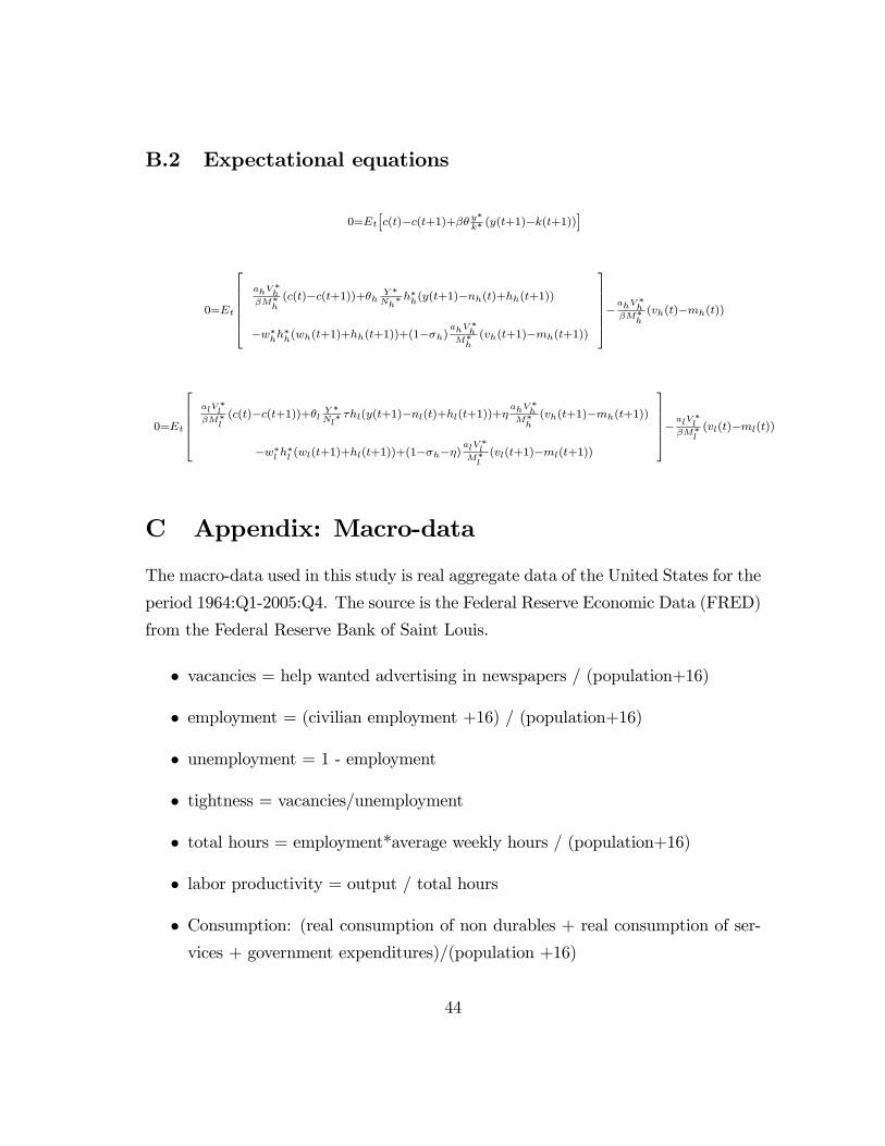
B.2 Expectational equations

0=Et[c(t)�c(t+1)+�� y�k� (y(t+1)�k(t+1))]

0=Et

2666664ahV

�h

�M�h(c(t)�c(t+1))+�h Y �

Nh� h�h(y(t+1)�nh(t)+hh(t+1))

�w�hh�h(wh(t+1)+hh(t+1))+(1��h)ahV

�h

M�h(vh(t+1)�mh(t+1))

3777775�ahV

�h

�M�h(vh(t)�mh(t))

0=Et

266664alV

�l

�M�l(c(t)�c(t+1))+�l Y

�Nl� �hl(y(t+1)�nl(t)+hl(t+1))+�

ahV�h

M�h(vh(t+1)�mh(t+1))

�w�l h�l (wl(t+1)+hl(t+1))+(1��h��)alV

�l

M�l(vl(t+1)�ml(t+1))

377775�alV�l

�M�l(vl(t)�ml(t))

C Appendix: Macro-data

The macro-data used in this study is real aggregate data of the United States for the

period 1964:Q1-2005:Q4. The source is the Federal Reserve Economic Data (FRED)

from the Federal Reserve Bank of Saint Louis.

� vacancies = help wanted advertising in newspapers / (population+16)

� employment = (civilian employment +16) / (population+16)

� unemployment = 1 - employment

� tightness = vacancies/unemployment

� total hours = employment*average weekly hours / (population+16)

� labor productivity = output / total hours

� Consumption: (real consumption of non durables + real consumption of ser-vices + government expenditures)/(population +16)

44

� Investment = (real consumption of durable goods+ real �xed private invest-

ment)/(population +16)

� output = consumption + investment + vacancies*cost per vacancy

� Normalization of output

� output =1

� consumption = Consumption / output

� investment = Investment / output

45