�

�

�

�

�

�

�

�

10

Ray Tracing

Ray tracing is a method to produce realistic images; it determines visible sur-faces in an image at the pixel level (Appel, 1968; Kay & Greenberg, 1979; Whit-ted, 1980). Unlike the z-buffer and BSP tree, ray tracing operates pixel-by-pixelrather than primitive-by-primitive. This tends to make ray tracing relatively slowfor scenes with large objects in screen space. However, it has a variety of nicefeatures which often make it the right choice for batch rendering and even forsome interactive applications.

Ray tracing’s primary benefit is that it is relatively straightforward to com-pute shadows and reflections. In addition, ray tracing is well suited to “walk-throughs” of extremely large models due to advanced ray tracing’s low asymptotictime complexity which makes up for the required preprocessing of the model(Snyder & Barr, 1987; Muuss, 1995; Parker, Martin, et al., 1999; Wald, Slusallek,Benthin, & Wagner, 2001).

In an interactive 3D program implemented in a conventional z-buffer environ-ment, it is often useful to be able to select an object using a mouse. The mouse isclicked in pixel (i, j) and the “picked” object is whatever object is “seen” throughthat pixel. If the rasterization process includes an object identification buffer, thisis just a matter of looking up the value in pixel (i, j) of that buffer. However,if that buffer is not available, we can solve the problem of which object is vis-ible via brute force geometrical computation using a “ray intersection test.” Inthis way, ray tracing is useful also to programmers who use only standardgraphics APIs.

201

�

�

�

�

�

�

�

�

202 10. Ray Tracing

This chapter also discusses distribution ray tracing (Cook, Porter, & Carpen-ter, 1984), where multiple random rays are sent through each pixel in an image tosimultaneously solve the antialiasing, soft shadow, fuzzy reflection, and depth-of-field problems.

10.1 The Basic Ray-Tracing Algorithm

The simplest use of ray tracing is to produce images similar to those producedby the z-buffer and BSP-tree algorithms. Fundamentally, those methods makesure the appropriate object is “seen” through each pixel,and that the pixel color isshaded based on that object’s material properties, the surface normal seen throughthat pixel, and the light geometry.

Figure 10.1. The 3D window we look through is the same as in Chapter 7. The borders ofthe window have simple coordinates in the uvw-coordinate system with respect to origin e.

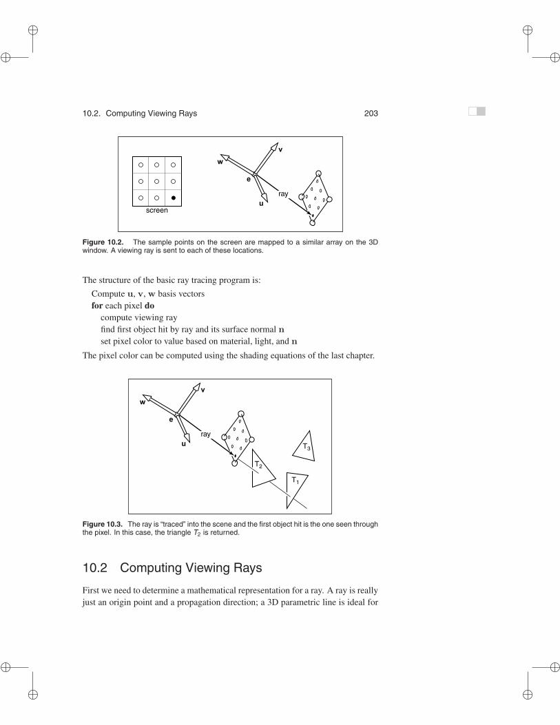
Figure 10.1 shows the basic viewing geometry for ray tracing, which is thesame as we saw earlier in Chapter 7. The geometry is aligned to a uvw coordinatesystem with the origin at the eye location e. The key idea in ray tracing is toidentify locations on the view plane at w = n that correspond to pixel centers, asshown in Figure 10.2. A “ray,” really just a directed 3D line, is then sent frome to that point. We then “gaze” in the direction of the ray to see the first objectseen in that direction. This is shown in Figure 10.3, where the ray intersects twotriangles, but only the first triangle hit, T2, is returned.

�

�

�

�

�

�

�

�

10.2. Computing Viewing Rays 203

Figure 10.2. The sample points on the screen are mapped to a similar array on the 3Dwindow. A viewing ray is sent to each of these locations.

The structure of the basic ray tracing program is:

Compute u, v, w basis vectorsfor each pixel do

compute viewing rayfind first object hit by ray and its surface normal nset pixel color to value based on material, light, and n

The pixel color can be computed using the shading equations of the last chapter.

Figure 10.3. The ray is “traced” into the scene and the first object hit is the one seen throughthe pixel. In this case, the triangle T2 is returned.

10.2 Computing Viewing Rays

First we need to determine a mathematical representation for a ray. A ray is reallyjust an origin point and a propagation direction; a 3D parametric line is ideal for

�

�

�

�

�

�

�

�

204 10. Ray Tracing

this. As discussed in Section 2.8.1, the 3D parametric line from the eye e to apoint s on the screen (see Figure 10.4) is given by

Figure 10.4. The ray fromthe eye to a point on thescreen.

p(t) = e + t(s− e).

This should be interpreted as, “we advance from e along the vector (s − e) afractional distance t to find the point p.” So given t, we can determine a point p.Note that p(0) = e, and p(1) = s. Also note that for positive t, if t1 < t2, thenp(t1) is closer to the eye than p(t2). Also, if t < 0, then p(t) is “behind” the eye.These facts will be useful when we search for the closest object hit by the ray thatis not behind the eye. Note that we are overloading the variable t here which isalso used for the top of the screen’s v-coordinate.

To compute a viewing ray, we need to know e (which is given) and s. Findings may look somewhat difficult. In fact, it is relatively straightforward using thesame transform machinery we used for viewing in the context of projecting linesand triangles.

First, we find the coordinates of s in the uvw-coordinate system with origin e.For all points on the screen, ws = n as shown in Figure 10.2. The uv-coordinatesare found by the windowing transform that takes [−0.5, nx−0.5]×[−0.5, ny−0.5]to [l, r]× [b, t]:

us = l + (r − l)i + 0.5

nx,

vs = b + (t− b)j + 0.5

ny,

where (i, j) are the pixel indices. This gives us s in uvw-coordinates. By defini-tion, we can convert to canonical coordinates:

s = e + usu + vsv + wsw. (10.1)

Alternatively, we could use the matrix form (Equation 6.8):

xs

ys

zs

1

=

1 0 0 xe

0 1 0 ye

0 0 1 ze

0 0 0 1

xu xv xw 0yu yv yw 0zu zv zw 00 0 0 1

us

vs

ws

1

, (10.2)

which is just the matrix form of Equation 10.1. We can compose this with thewindowing transform in matrix form if we wished, but this is probably not worthdoing unless you like the matrix form of equations better.

�

�

�

�

�

�

�

�

10.3. Ray-Object Intersection 205

10.3 Ray-Object Intersection

Given a ray e + td, we want to find the first intersection with any object wheret > 0. It will later prove useful to solve a slightly more general problem offinding the first intersection in the interval [t0, t1], and using [0,∞) for viewingrays. We solve this for both spheres and triangles in this section. In the nextsection, multiple objects are discussed.

10.3.1 Ray-Sphere Intersection

Given a ray p(t) = e + td and an implicit surface f(p) = 0, we’d like to knowwhere they intersect. The intersection points occur when points on the ray satisfythe implicit equation

f(p(t)) = 0.

This is justf(e + td) = 0.

A sphere with center c = (xc, yc, zc) and radius R can be represented by theimplicit equation

(x− xc)2 + (y − yc)2 + (z − zc)2 −R2 = 0.

We can write this same equation in vector form:

(p− c) · (p− c)−R2 = 0.

Any point p that satisfies this equation is on the sphere. If we plug points on theray p(t) = e + td into this equation, we can solve for the values of t on the raythat yield points on the sphere:

(e + td− c) · (e + td− c)−R2 = 0.

Rearranging terms yields

(d · d)t2 + 2d · (e− c)t + (e− c) · (e− c)−R2 = 0.

Here, everything is known except the parameter t, so this is a classic quadraticequation in t, meaning it has the form

At2 + Bt + C = 0.

The solution to this equation is discussed in Section 2.2. The term under thesquare root sign in the quadratic solution, B2 − 4AC, is called the discriminant

�

�

�

�

�

�

�

�

206 10. Ray Tracing

and tells us how many real solutions there are. If the discriminant is negative, itssquare root is imaginary and there are no intersections between the sphere and theline. If the discriminant is positive, there are two solutions: one solution wherethe ray enters the sphere and one where it leaves. If the discriminant is zero, theray grazes the sphere touching it at exactly one point. Plugging in the actual termsfor the sphere and eliminating the common factors of two, we get

t =−d · (e− c)±

√(d · (e− c))2 − (d · d) ((e− c) · (e− c)−R2)

(d · d).

In an actual implementation, you should first check the value of the discriminantbefore computing other terms. If the sphere is used only as a bounding object formore complex objects, then we need only determine whether we hit it; checkingthe discriminant suffices.

As discussed in Section 2.7.1, the normal vector at point p is given by thegradient n = 2(p− c). The unit normal is (p− c)/R.

10.3.2 Ray-Triangle Intersection

There are many algorithms for computing ray-triangle intersections. We will usethe form that uses barycentric coordinates for the parametric plane containing thetriangle, because it requires no long-term storage other than the vertices of thetriangle (Snyder & Barr, 1987).

To intersect a ray with a parametric surface, we set up a system of equationswhere the Cartesian coordinates all match:

xe + txd = f(u, v),

ye + tyd = g(u, v),

ze + tzd = h(u, v).

Here, we have three equations and three unknowns (t, u, and v), so we can solvenumerically for the unknowns. If we are lucky, we can solve for them analytically.

Figure 10.5. The ray hitsthe plane containing the tri-angle at point p.

In the case where the parametric surface is a parametric plane, the parametricequation can be written in vector form as discussed in Section 2.11.2. If thevertices of the triangle are a, b and c, then the intersection will occur when

e + td = a + β(b− a) + γ(c− a). (10.3)

The hitpoint p will be at e + td as shown in Figure 10.5. Again, from Sec-tion 2.11.2, we know the hitpoint is in the triangle if and only if β > 0, γ > 0,

�

�

�

�

�

�

�

�

10.3. Ray-Object Intersection 207

and β + γ < 1. Otherwise, it hits the plane outside the triangle. If there areno solutions, either the triangle is degenerate or the ray is parallel to the planecontaining the triangle.

To solve for t, β, and γ in Equation 10.3, we expand it from its vector forminto the three equations for the three coordinates:

xe + txd = xa + β(xb − xa) + γ(xc − xa),

ye + tyd = ya + β(yb − ya) + γ(yc − ya),

ze + tzd = za + β(zb − za) + γ(zc − za).

This can be rewritten as a standard linear equation:xa − xb xa − xc xd

ya − yb ya − yc yd

za − zb za − zc zd

β

γt

=

xa − xe

ya − ye

za − ze

.

The fastest classic method to solve this 3× 3 linear system is Cramer’s rule. Thisgives us the solutions

β =

∣∣∣∣∣∣xa − xe xa − xc xd

ya − ye ya − yc yd

za − ze za − zc zd

∣∣∣∣∣∣|A| ,

γ =

∣∣∣∣∣∣xa − xb xa − xe xd

ya − yb ya − ye yd

za − zb za − ze zd

∣∣∣∣∣∣|A| ,

t =

∣∣∣∣∣∣xa − xb xa − xc xa − xe

ya − yb ya − yc ya − ye

za − zb za − zc za − ze

∣∣∣∣∣∣|A| ,

where the matrix A is

A =

xa − xb xa − xc xd

ya − yb ya − yc yd

za − zb za − zc zd

,

and |A| denotes the determinant of A. The 3×3 determinants have common sub-terms that can be exploited. Looking at the linear systems with dummy variables

a d gb e hc f i

β

γt

=

j

kl

,

�

�

�

�

�

�

�

�

208 10. Ray Tracing

Cramer’s rule gives us

β =j(ei− hf) + k(gf − di) + l(dh− eg)

M,

γ =i(ak − jb) + h(jc− al) + g(bl − kc)

M,

t = −f(ak − jb) + e(jc− al) + d(bl − kc)M

,

whereM = a(ei− hf) + b(gf − di) + c(dh− eg).

We can reduce the number of operations by reusing numbers such as“ei-minus-hf.”

The algorithm for the ray-triangle intersection for which we need the linear so-lution can have some conditions for early termination. Thus, the function shouldlook something like:

boolean raytri (ray r, vector3 a, vector3 b, vector3 c, interval [t0, t1])compute t

if (t < t0) or (t > t1) thenreturn false

compute γ

if (γ < 0) or (γ > 1) thenreturn false

compute β

if (β < 0) or (β > 1− γ) thenreturn false

return true

10.3.3 Ray-Polygon Intersection

Given a polygon with m vertices p1 through pm and surface normal n, we firstcompute the intersection points between the ray e + td and the plane containingthe polygon with implicit equation

(p− p1) · n = 0.

We do this by setting p = e + td and solving for t to get

t =(p1 − e) · n

d · n .

�

�

�

�

�

�

�

�

10.4. A Ray-Tracing Program 209

This allows us to compute p. If p is inside the polygon, then the ray hits it, andotherwise it does not.

We can answer the question of whether p is inside the polygon by projectingthe point and polygon vertices to the xy plane and answering it there. The easiestway to do this is to send any 2D ray out from p and to count the number ofintersections between that ray and the boundary of the polygon (Sutherland et al.,1974; Glassner, 1989). If the number of intersections is odd, then the point isinside the polygon, and otherwise it is not. This is true, because a ray that goesin must go out, thus creating a pair of intersections. Only a ray that starts insidewill not create such a pair. To make computation simple, the 2D ray may as wellpropagate along the x-axis:

[xy

]=[xp

yp

]+ s

[10

].

It is straightforward to compute the intersection of that ray with the edges such as(x1, y1, x2, y2) for s ∈ (0,∞).

A problem arises, however, for polygons whose projection into the xy planeis a line. To get around this, we can choose among the xy, yz, or zx planes forwhichever is best. If we implement our points to allow an indexing operation,e.g., p(0) = xp then this can be accomplished as follows:

if (abs(zn) > abs(xn)) and (abs(zn) > abs(xn)) thenindex0 = 0index1 = 1

else if (abs(yn) > abs (xn)) thenindex0 = 0index1 = 2

elseindex0 = 1index1 = 2

Now, all computations can use p(index0) rather than xp, and so on.

10.4 A Ray-Tracing Program

We now know how to generate a viewing ray for a given pixel and how to findthe intersection with one object. This can be easily extended to a program thatproduces images similar to the z-buffer or BSP-tree codes of earlier chapters:

�

�

�

�

�

�

�

�

210 10. Ray Tracing

for each pixel docompute viewing rayif (ray hits an object with t ∈ [0,∞)) then

Compute nEvaluate lighting equation and set pixel to that color

elseset pixel color to background color

Here the statement “if ray hits an object...” can be implemented as a function thattests for hits in the interval t ∈ [t0, t1]:

hit = falsefor each object o do

if (object is hit at ray parameter t and t ∈ [t0, t1]) thenhit = truehitobject = ot1 = t

return hit

In an actual implementation, you will need to somehow return either a referenceto the object that is hit or at least its normal vector and material properties. Thisis often done by passing a record/structure with such information. In an object-oriented implementation, it is a good idea to have a class called something likesurface with derived classes triangle, sphere, surface-list, etc. Anything that aray can intersect would be under that class. The ray tracing program would thenhave one reference to a “surface” for the whole model, and new types of objectsand efficiency structures can be added transparently.

10.4.1 Object-Oriented Design for a Ray-Tracing Program

As mentioned earlier, the key class hierarchy in a ray tracer are the geometricobjects that make up the model. These should be subclasses of some geometricobject class, and they should support a hit function (Kirk & Arvo, 1988). Toavoid confusion from use of the word “object,” surface is the class name oftenused. With such a class, you can create a ray tracer that has a general interfacethat assumes little about modeling primitives and debug it using only spheres. Animportant point is that anything that can be “hit” by a ray should be part of thisclass hierarchy, e.g., even a collection of surfaces should be considered a subclassof the surface class. This includes efficiency structures, such as bounding volumehierarchies; they can be hit by a ray, so they are in the class.

�

�

�

�

�

�

�

�

10.5. Shadows 211

For example, the “abstract” or “base” class would specify the hit function aswell as a bounding box function that will prove useful later:

class surfacevirtual bool hit(ray e + td, real t0, real t1, hit-record rec)virtual box bounding-box()

Here (t0, t1) is the interval on the ray where hits will be returned, and rec isa record that is passed by reference; it contains data such as the t at intersectionwhen hit returns true. The type box is a 3D “bounding box”, that is two points thatdefine an axis-aligned box that encloses the surface. For example, for a sphere,the function would be implemented by:

box sphere::bounding-box()vector3 min = center - vector3(radius,radius,radius)vector3 max = center + vector3(radius,radius,radius)return box(min, max)

Another class that is useful is material. This allows you to abstract the materialbehavior and later add materials transparently. A simple way to link objects andmaterials is to add a pointer to a material in the surface class, although moreprogrammable behavior might be desirable. A big question is what to do withtextures; are they part of the material class or do they live outside of the materialclass? This will be discussed more in Chapter 11.

10.5 Shadows

Once you have a basic ray tracing program, shadows can be added very easily.Recall from Chapter 9 that light comes from some direction l. If we imagineourselves at a point p on a surface being shaded, the point is in shadow if we“look” in direction l and see an object. If there are no objects, then the light is notblocked.

This is shown in Figure 10.6, where the ray p + tl does not hit any objectsand is thus not in shadow. The point q is in shadow because the ray q + tl doeshit an object. The vector l is the same for both points because the light is “far”away. This assumption will later be relaxed. The rays that determine in or out ofshadow are called shadow rays to distinguish them from viewing rays.

Figure 10.6. The point pis not in shadow while thepoint q is in shadow.

To get the algorithm for shading, we add an if statement to determine whetherthe point is in shadow. In a naive implementation, the shadow ray will checkfor t ∈ [0,∞), but because of numerical imprecision, this can result in an inter-

�

�

�

�

�

�

�

�

212 10. Ray Tracing

section with the surface on which p lies. Instead, the usual adjustment to avoidthat problem is to test for t ∈ [ε,∞) where ε is some small positive constant(Figure 10.7).

Figure 10.7. By testingin the interval starting at ε,we avoid numerical impre-cision causing the ray to hitthe surface p is on.

If we implement shadow rays for Phong lighting with Equation 9.9 then wehave:

function raycolor( ray e + td, real t0, real t1 )hit-record rec, srecif (scene→hit(e + td, t0, t1, rec)) then

p = e + rec.tdcolor c = rec.cr rec.ca

if (not scene→hit(p + sl, ε,∞, srec)) thenvector3 h = normalized(normalized(l) + normalized(−d))c = c + rec.cr clmax (0, rec.n · l) + clrec.cp(h · rec.n)rec.p

return c

elsereturn background-color

Note that the ambient color is added in either case. If there are multiple lightsources, we can send a shadow ray and evaluate the diffuse/phong terms for eachlight. The code above assumes that d and l are not necessarily unit vectors. Thisis crucial for d, in particular, if we wish to cleanly add instancing later.

10.6 Specular Reflection

It is straightforward to add specular reflection to a ray-tracing program. The keyobservation is shown in Figure 10.8 where a viewer looking from direction esees what is in direction r as seen from the surface. The vector r is found usinga variant of the Phong lighting reflection Equation 9.6. There are sign changesbecause the vector d points toward the surface in this case, so,

r = d + 2(d · n)n, (10.4)

In the real world, some energy is lost when the light reflects from the surface, andFigure 10.8. When look-ing into a perfect mirror, theviewer looking in direction dwill see whatever the viewer“below” the surface wouldsee in direction r.

this loss can be different for different colors. For example, gold reflects yellowmore efficiently than blue, so it shifts the colors of the objects it reflects. This canbe implemented by adding a recursive call in raycolor:

color c = c + csraycolor(p + sr, ε,∞)

where cs is the specular RGB color. We need to make sure we test for s ∈ [ε,∞)

�

�

�

�

�

�

�

�

10.7. Refraction 213

for the same reason as we did with shadow rays; we don’t want the reflection rayto hit the object that generates it.

The problem with the recursive call above is that it may never terminate. Forexample, if a ray starts inside a room, it will bounce forever. This can be fixed byadding a maximum recursion depth. The code will be more efficient if a reflectionray is generated only if cs is not zero (black).

10.7 Refraction

Another type of specular object is a dielectric—a transparent material that refractslight. Diamonds, glass, water, and air are dielectrics. Dielectrics also filter light;some glass filters out more red and blue light than green light, so the glass takeson a green tint. When a ray travels from a medium with refractive index n intoone with a refractive index nt, some of the light is transmitted, and it bends. Thisis shown for nt > n in Figure 10.9. Snell’s law tells us that

n sin θ = nt sin φ.

Computing the sine of an angle between two vectors is usually not as convenientas computing the cosine which is a simple dot product for the unit vectors such aswe have here. Using the trigonometric identity sin2 θ +cos2 θ = 1, we can derivea refraction relationship for cosines:

cos2 φ = 1− n2(1− cos2 θ

)n2

t

.

Note that if n and nt are reversed, then so are θ and φ as shown on the right ofFigure 10.9.

Figure 10.9. Snell’s Law describes how the angle φ depends on the angle θ and therefractive indices of the object and the surrounding medium.

�

�

�

�

�

�

�

�

214 10. Ray Tracing

To convert sinφ and cos φ into a 3D vector, we can set up a 2D orthonormalbasis in the plane of n and d.

From Figure 10.10, we can see that n and b form an orthonormal basis for theplane of refraction. By definition, we can describe t in terms of this basis:

t = sinφb− cos φn.

Since we can describe d in the same basis, and d is known, we can solve for b:

d = sin θb− cos θn,

b =d + n cos θ

sin θ.

This means that we can solve for t with known variables:Figure 10.10. The vectorsn and b form a 2D orthonor-mal basis that is parallel tothe transmission vector t.

t =n (d + n cos θ))

nt− n cos φ

=n (d− n(d · n))

nt− n

√1− n2 (1− (d · n)2)

n2t

.

Note that this equation works regardless of which of n and nt is larger. An im-mediate question is, “What should you do if the number under the square root isnegative?” In this case, there is no refracted ray and all of the energy is reflected.This is known as total internal reflection, and it is responsible for much of therich appearance of glass objects.

The reflectivity of a dielectric varies with the incident angle according to theFresnel equations. A nice way to implement something close to the Fresnel equa-tions is to use the Schlick approximation (Schlick, 1994a),

R(θ) = R0 + (1−R0) (1− cos θ)5 ,

where R0 is the reflectance at normal incidence:

R0 =(

nt − 1nt + 1

)2

.

Note that the cos θ terms above are always for the angle in air (the larger of theinternal and external angles relative to the normal).

For homogeneous impurities, as is found in typical glass, a light-carrying ray’sintensity will be attenuated according to Beer’s Law. As the ray travels throughthe medium it loses intensity according to dI = −CI dx, where dx is distance.Thus, dI/dx = −CI . We can solve this equation and get the exponential I =k exp(−Cx)+k′. The degree of attenuation is described by the RGB attenuation

�

�

�

�

�

�

�

�

10.7. Refraction 215

Figure 10.11. The color of the glass is affected by total internal reflection and Beer’s Law.The amount of light transmitted and reflected is determined by the Fresnel equations. Thecomplex lighting on the ground plane was computed using particle tracing as described inChapter 23. (See also Plate VI.)

constant a, which is the amount of attenuation after one unit of distance. Puttingin boundary conditions, we know that I(0) = I0, and I(1) = aI(0). The formerimplies I(x) = I0 exp(−Cx). The latter implies I0a = I0 exp(−C), so −C =ln(a). Thus, the final formula is

I(s) = I(0)e− ln(a)s,

where I(s) is the intensity of the beam at distance s from the interface. In practice,we reverse-engineer a by eye, because such data is rarely easy to find. The effectof Beer’s Law can be seen in Figure 10.11, where the glass takes on a green tint.

To add transparent materials to our code, we need a way to determine whena ray is going “into” an object. The simplest way to do this is to assume that allobjects are embedded in air with refractive index very close to 1.0, and that surfacenormals point “out” (toward the air). The code segment for rays and dielectricswith these assumptions is:

if (p is on a dielectric) thenr = reflect(d, n )if (d · n < 0) then

refract(d, n,n, t )

�

�

�

�

�

�

�

�

216 10. Ray Tracing

c = −d · nkr = kg = kb = 1

elsekr = exp(−art)kg = exp(−agt)kb = exp(−abt)if refract(d, -n,1/n, t ) then

c = t · nelse

return k∗color(p + tr)R0 = (n− 1)2/(n + 1)2

R = R0 + (1−R0)(1− c)5

return k(R color(p + tr) + (1−R) color(p + tt))

The code above assumes that the natural log has been folded into the constants(ar, ag, ab). The refract function returns false if there is total internal reflection,and otherwise it fills in the last argument of the argument list.

10.8 Instancing

An elegant property of ray tracing is that it allows very natural instancing. Thebasic idea of instancing is to distort all points on an object by a transformationmatrix before the object is displayed. For example, if we transform the unit circle(in 2D) by a scale factor (2, 1) in x and y, respectively, then rotate it by 45◦, andmove one unit in the x-direction, the result is an ellipse with an eccentricity of 2and a long axis along the x = −y-direction centered at (0, 1) (Figure 10.12). Thekey thing that makes that entity an “instance” is that we store the circle and thecomposite transform matrix. Thus, the explicit construction of the ellipse is leftas a future procedure operation at render time.

Figure 10.12. An instanceof a circle with a series ofthree transforms is an el-lipse.

The advantage of instancing in ray tracing is that we can choose the spacein which to do intersection. If the base object is composed of a set of points,one of which is p, then the transformed object is composed of that set of pointstransformed by matrix M, where the example point is transformed to Mp. If wehave a ray a + tb which we want to intersect with the transformed object, we caninstead intersect an inverse-transformed ray with the untransformed object (Fig-ure 10.13). There are two potential advantages to computing in the untransformedspace (i.e., the right-hand side of Figure 10.13):

1. the untransformed object may have a simpler intersection routine, e.g., asphere versus an ellipsoid;

�

�

�

�

�

�

�

�

10.8. Instancing 217

Figure 10.13. The ray intersection problem in the two spaces are just simple transformsof each other. The object is specified as a sphere plus matrix M. The ray is specified in thetransformed (world) space by location a and direction b.

2. many transformed objects can share the same untransformed object thusreducing storage, e.g., a traffic jam of cars, where individual cars are justtransforms of a few base (untransformed) models.

As discussed in Section 6.2.2, surface normal vectors transform differently.With this in mind and using the concepts illustrated in Figure 10.13, we can de-termine the intersection of a ray and an object transformed by matrix M. If wecreate an instance class of type surface, we need to create a hit function:

instance::hit(ray a + tb, real t0, real t1, hit-record rec)ray r′ = M−1a + tM−1bif (base-object→hit(r′, t0, t1, rec)) then

rec.n = (M−1)T rec.nreturn true

elsereturn false

An elegant thing about this function is that the parameter rec.t does not need tobe changed, because it is the same in either space. Also note that we need notcompute or store the matrix M.

�

�

�

�

�

�

�

�

218 10. Ray Tracing

This brings up a very important point: the ray direction b must not be re-stricted to a unit-length vector, or none of the infrastructure above works. For thisreason, it is useful not to restrict ray directions to unit vectors.

For the purpose of solid texturing, you may want to record the local coordi-nates of the hitpoint and return this in the hit-record. This is just ray r′ advancedby parameter rec.t.

To implement the bounding-box function of class instance, we can just takethe eight corners of the bounding box of the base object and transform all ofthem by M, and then take the bounding box of those eight points. That will notnecessarily yield the tightest bounding box, but it is general and straightforwardto implement.

10.9 Sub-Linear Ray-Object Intersection

In the earlier ray-object intersection pseudocode, all objects are looped over,checking for intersections. For N objects, this is an O(N) linear search andis thus slow for large values of N . Like most search problems, the ray-objectintersection can be computed in sub-linear time using “divide and conquer” tech-niques, provided we can create an ordered data structure as a preprocess. Thereare many techniques to do this.

This section discusses three of these techniques in detail: bounding volumehierarchies (Rubin & Whitted, 1980; Whitted, 1980; Goldsmith & Salmon, 1987),uniform spatial subdivision (Cleary, Wyvill, Birtwistle, & Vatti, 1983; Fujimoto,Tanaka, & Iwata, 1986; Amanatides & Woo, 1987), and binary space partition-

Figure 10.14. Left: a uniform partitioning of space. Right: adaptive bounding-box hierarchy.Image courtesy David DeMarle.

�

�

�

�

�

�

�

�

10.9. Sub-Linear Ray-Object Intersection 219

ing (Glassner, 1984; Jansen, 1986; Havran, 2000). An example of the first twostrategies is shown in Figure 10.14.

10.9.1 Bounding Boxes

A key operation in most intersection acceleration schemes is computing the inter-section of a ray with a bounding box (Figure 10.15). This differs from conven-tional intersection tests in that we do not need to know where the ray hits the box;we only need to know whether it hits the box.

To build an algorithm for ray-box intersection, we begin by considering a 2Dray whose direction vector has positive x and y components. We can generalizethis to arbitrary 3D rays later. The 2D bounding box is defined by two horizontaland two vertical lines:

Figure 10.15. The ray isonly tested for intersectionwith the surfaces if it hits thebounding box.

x = xmin,

x = xmax,

y = ymin,

y = ymax.

The points bounded by these lines can be described in interval notation:

(x, y) ∈ [xmin, xmax]× [ymin, ymax].

As shown in Figure 10.16, the intersection test can be phrased in terms of theseintervals. First, we compute the ray parameter where the ray hits the line x =xmin:

txmin =xmin − xe

xd.

We then make similar computations for txmax, tymin, and tymax. The ray hits thebox if and only if the intervals [txmin, txmax] and [tymin, tymax] overlap, i.e., theirintersection is non-empty. In pseudocode this algorithm is:

txmin = (xmin − xe)/xd

txmax = (xmax − xe)/xd

tymin = (ymin − ye)/yd

tymax = (ymax − ye)/yd

if (txmin > tymax) or (tymin > txmax) thenreturn false

elsereturn true

�

�

�

�

�

�

�

�

220 10. Ray Tracing

Figure 10.16. The ray will be inside the interval x ∈ [xmin, xmax] for some interval in itsparameter space t ∈ [txmin, txmax]. A similar interval exists for the y interval. The ray intersectsthe box if it is in both the x interval and y interval at the same time, i.e., the intersection of thetwo one-dimensional intervals is not empty.

The if statement may seem non-obvious. To see the logic of it, note that there isno overlap if the first interval is either entirely to the right or entirely to the left ofthe second interval.

The first thing we must address is the case when xd or yd is negative. If xd isnegative, then the ray will hit xmax before it hits xmin. Thus the code for computingtxmin and txmax expands to:

if (xd ≥ 0) thentxmin = (xmin − xe)/xd

txmax = (xmax − xe)/xd

elsetxmin = (xmax − xe)/xd

txmax = (xmin − xe)/xd

A similar code expansion must be made for the y cases. A major concern is thathorizontal and vertical rays have a zero value for yd and xd, respectively. Thiswill cause divide by zero which may be a problem. However, before addressingthis directly, we check whether IEEE floating point computation handles these

�

�

�

�

�

�

�

�

10.9. Sub-Linear Ray-Object Intersection 221

cases gracefully for us. Recall from Section 1.6 the rules for divide by zero: forany positive real number a,

+a/0 = +∞;

−a/0 = −∞.

Consider the case of a vertical ray where xd = 0 and yd > 0. We can thencalculate

txmin =xmin − xe

0;

txmax =xmax − xe

0.

There are three possibilities of interest:

1. xe ≤ xmin (no hit);

2. xmin < xe < xmax (hit);

3. xmax ≤ xe (no hit).

For the first case we have

txmin =positive number

0;

txmax =positive number

0.

This yields the interval (txmin, txmin) = (∞,∞). That interval will not overlapwith any interval, so there will be no hit, as desired. For the second case, we have

txmin =negative number

0;

txmax =positive number

0.

This yields the interval (txmin, txmin) = (−∞,∞) which will overlap with allintervals and thus will yield a hit as desired. The third case results in the interval(−∞,−∞) which yields no hit, as desired. Because these cases work as desired,we need no special checks for them. As is often the case, IEEE floating pointconventions are our ally. However, there is still a problem with this approach.

�

�

�

�

�

�

�

�

222 10. Ray Tracing

Consider the code segment:

if (xd ≥ 0) thentmin = (xmin − xe)/xd

tmax = (xmax − xe)/xd

elsetmin = (xmax − xe)/xd

tmax = (xmin − xe)/xd

This code breaks down when xd = −0. This can be overcome by testing on thereciprocal of xd (A. Williams, Barrus, Morley, & Shirley, 2005):

a = 1/xd

if (a ≥ 0) thentmin = a(xmin − xe)tmax = a(xmax − xe)

elsetmin = a(xmax − xe)tmax = a(xmin − xe)

10.9.2 Hierarchical Bounding Boxes

The basic idea of hierarchical bounding boxes can be seen by the common tacticof placing an axis-aligned 3D bounding box around all the objects as shown inFigure 10.17. Rays that hit the bounding box will actually be more expensiveto compute than in a brute force search, because testing for intersection with thebox is not free. However, rays that miss the box are cheaper than the brute forcesearch. Such bounding boxes can be made hierarchical by partitioning the set of

Figure 10.17. A 2D ray e+ t d is tested against a 2Dbounding box.

Figure 10.18. The bound-ing boxes can be nested bycreating boxes around sub-sets of the model.

objects in a box and placing a box around each partition as shown in Figure 10.18.The data structure for the hierarchy shown in Figure 10.19 might be a tree withthe large bounding box at the root and the two smaller bounding boxes as left andright subtrees. These would in turn each point to a list of three triangles. Theintersection of a ray with this particular hard-coded tree would be:

if (ray hits root box) thenif (ray hits left subtree box) then

check three triangles for intersectionif (ray intersects right subtree box) then

check other three triangles for intersectionif (an intersections returned from each subtree) then

return the closest of the two hits

�

�

�

�

�

�

�

�

10.9. Sub-Linear Ray-Object Intersection 223

else if (a intersection is returned from exactly one subtree) thenreturn that intersection

elsereturn false

elsereturn false

Some observations related to this algorithm are that there is no geometric orderingbetween the two subtrees, and there is no reason a ray might not hit both subtrees.Indeed, there is no reason that the two subtrees might not overlap.

A key point of such data hierarchies is that a box is guaranteed to bound allobjects that are below it in the hierarchy, but they are not guaranteed to containall objects that overlap it spatially, as shown in Figure 10.19. This makes thisgeometric search somewhat more complicated than a traditional binary search onstrictly ordered one-dimensional data. The reader may note that several possibleoptimizations present themselves. We defer optimizations until we have a fullhierarchical algorithm.

Figure 10.19. Thegrey box is a tree nodethat points to the three greyspheres, and the thick blackbox points to the three blackspheres. Note that not allspheres enclosed by thebox are guaranteed to bepointed to by the corre-sponding tree node.

If we restrict the tree to be binary and require that each node in the tree have abounding box, then this traversal code extends naturally. Further, assume that allnodes are either leaves in the tree and contain a primitive, or that they contain oneor two subtrees.

The bvh-node class should be of type surface, so it should implementsurface::hit. The data it contains should be simple:

class bvh-node subclass of surfacevirtual bool hit(ray e + td, real t0, real t1, hit-record rec)virtual box bounding-box()surface-pointer leftsurface-pointer rightbox bbox

The traversal code can then be called recursively in an object-oriented style:

bool bvh-node::hit(ray a + tb, real t0, real t1, hit-record rec)if (bbox.hitbox(a + tb, t0, t1)) then

hit-record lrec, rrecleft-hit = (left = NULL) and (left→ hit(a + tb, t0, t1, lrec))right-hit = (right = NULL) and (right→ hit(a + tb, t0, t1, rrec))if (left-hit and right-hit) then

if (lrec.t < rrec.t) thenrec = lrec

�

�

�

�

�

�

�

�

224 10. Ray Tracing

elserec = rrec

return trueelse if (left-hit) then

rec = lrecreturn true

else if (right-hit) thenrec = rrecreturn true

elsereturn false

elsereturn false

Note that because left and right point to surfaces rather than bvh-nodes specifi-cally, we can let the virtual functions take care of distinguishing between internaland leaf nodes; the appropriate hit function will be called. Note, that if the treeis built properly, we can eliminate the check for left being NULL. If we want toeliminate the check for right being NULL, we can replace NULL right pointerswith a redundant pointer to left. This will end up checking left twice, but willeliminate the check throughout the tree. Whether that is worth it will depend onthe details of tree construction.

There are many ways to build a tree for a bounding volume hierarchy. It isconvenient to make the tree binary, roughly balanced, and to have the boxes ofsibling subtrees not overlap too much. A heuristic to accomplish this is to sortthe surfaces along an axis before dividing them into two sublists. If the axes aredefined by an integer with x = 0, y = 1, and z = 2 we have:

bvh-node::bvh-node(object-array A, int AXIS)N = A.lengthif (N= 1) then

left = A[0]right = NULLbbox = bounding-box(A[0])

else if (N= 2) thenleft-node = A[0]right-node = A[1]bbox = combine(bounding-box(A[0]), bounding-box(A[1]))

elsesort A by the object center along AXIS

�

�

�

�

�

�

�

�

10.9. Sub-Linear Ray-Object Intersection 225

left= new bvh-node(A[0..N/2− 1], (AXIS +1) mod 3)right = new bvh-node(A[N/2..N−1], (AXIS +1) mod 3)bbox = combine(left-node→ bbox, right-node→ bbox)

The quality of the tree can be improved by carefully choosing AXIS each time.One way to do this is to choose the axis such that the sum of the volumes of thebounding boxes of the two subtrees is minimized. This change compared to ro-tating through the axes will make little difference for scenes composed of isotopi-cally distributed small objects, but it may help significantly in less well-behavedscenes. This code can also be made more efficient by doing just a partition ratherthan a full sort.

Another, and probably better, way to build the tree is to have the subtreescontain about the same amount of space rather than the same number of objects.To do this we partition the list based on space:

bvh-node::bvh-node(object-array A, int AXIS)N = A.lengthif (N = 1) then

left = A[0]right = NULLbbox = bounding-box(A[0])

else if (N = 2) thenleft = A[0]right = A[1]bbox = combine(bounding-box(A[0]), bounding-box(A[1]))

elsefind the midpoint m of the bounding box of A along AXISpartition A into lists with lengths k and (N-k) surrounding m

left = new node(A[0..k], (AXIS +1) mod 3)right = new node(A[k+1..N−1], (AXIS +1) mod 3)bbox = combine(left-node→ bbox, right-node→ bbox)

Although this results in an unbalanced tree, it allows for easy traversal of emptyspace and is cheaper to build because partitioning is cheaper than sorting.

10.9.3 Uniform Spatial Subdivision

Another strategy to reduce intersection tests is to divide space. This is funda-mentally different from dividing objects as was done with hierarchical boundingvolumes:

�

�

�

�

�

�

�

�

226 10. Ray Tracing

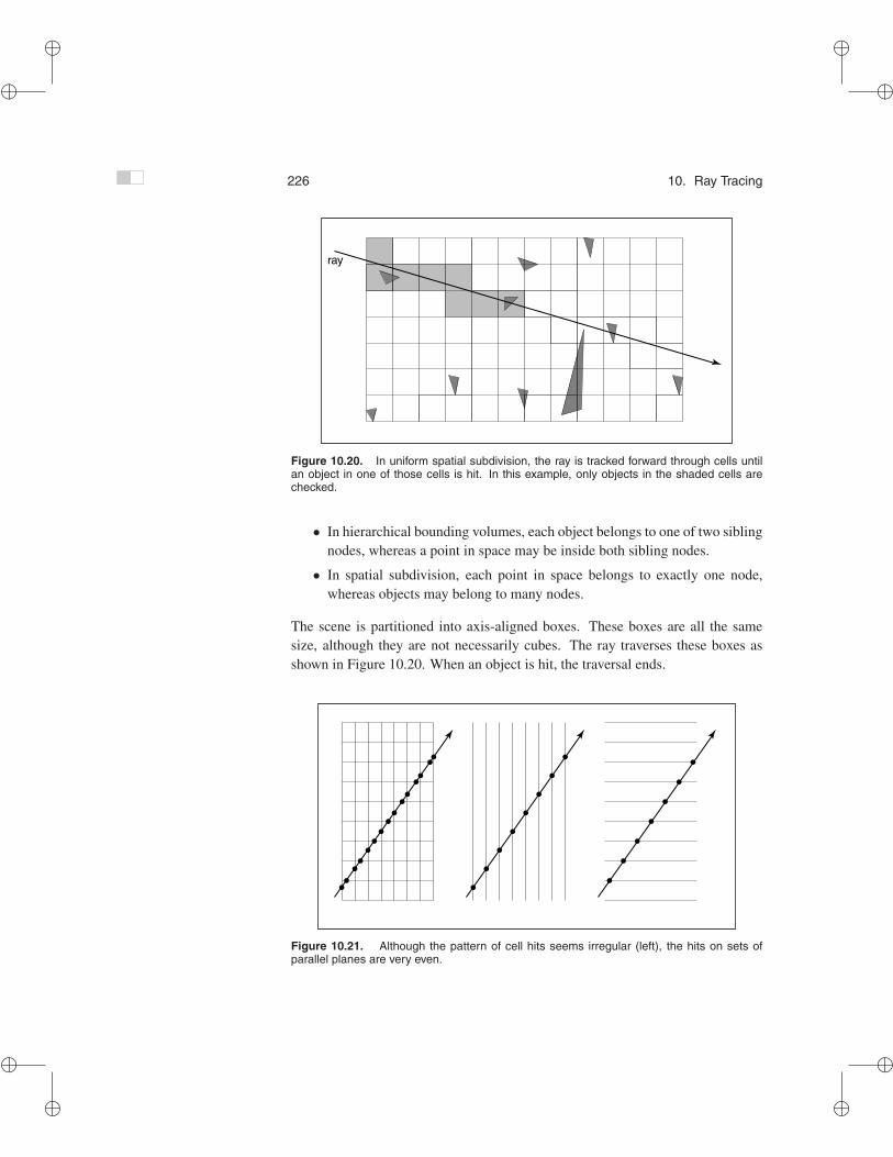
Figure 10.20. In uniform spatial subdivision, the ray is tracked forward through cells untilan object in one of those cells is hit. In this example, only objects in the shaded cells arechecked.

• In hierarchical bounding volumes, each object belongs to one of two siblingnodes, whereas a point in space may be inside both sibling nodes.

• In spatial subdivision, each point in space belongs to exactly one node,whereas objects may belong to many nodes.

The scene is partitioned into axis-aligned boxes. These boxes are all the samesize, although they are not necessarily cubes. The ray traverses these boxes asshown in Figure 10.20. When an object is hit, the traversal ends.

Figure 10.21. Although the pattern of cell hits seems irregular (left), the hits on sets ofparallel planes are very even.

�

�

�

�

�

�

�

�

10.9. Sub-Linear Ray-Object Intersection 227

The grid itself should be a subclass of surface and should be implemented asa 3D array of pointers to surface. For empty cells these pointers are NULL. Forcells with one object, the pointer points to that object. For cells with more thanone object, the pointer can point to a list, another grid, or another data structure,such as a bounding volume hierarchy.

Figure 10.22. To decidewhether we advance rightor upwards, we keep trackof the intersections with thenext vertical and horizontalboundary of the cell.

This traversal is done in an incremental fashion. The regularity comes fromthe way that a ray hits each set of parallel planes, as shown in Figure 10.21. Tosee how this traversal works, first consider the 2D case where the ray directionhas positive x and y components and starts outside the grid. Assume the grid isbounded by points (xmin, ymin) and (xmax, ymax). The grid has nx by ny cells.

Our first order of business is to find the index (i, j) of the first cell hit bythe ray e + td. Then, we need to traverse the cells in an appropriate order. Thekey parts to this algorithm are finding the initial cell (i, j) and deciding whetherto increment i or j (Figure 10.22). Note that when we check for an intersectionwith objects in a cell, we restrict the range of t to be within the cell (Figure 10.23).Most implementations make the 3D array of type “pointer to surface.” To improvethe locality of the traversal, the array can be tiled as discussed in Section 13.4.

10.9.4 Binary-Space Partitioning

Figure 10.23. Only hitswithin the cell should be re-ported. Otherwise the caseabove would cause us to re-port hitting object b ratherthan object a.

We can also partition space in a hierarchical data structure such as a binary-space-partitioning tree (BSP tree). This is similar to the BSP tree used for a painter’salgorithm in Chapter 8, but it usually uses axis-aligned cutting planes for easierray intersection. A node in this structure might contain a single cutting plane anda left and right subtree. These subtrees would contain all objects on either side ofthe cutting plane. Objects that pass through the plane would be in each subtree.If we assume the cutting plane is parallel to the yz plane at x = D, then the nodeclass is:

class bsp-node subclass of surfacevirtual bool hit(ray e + td, real t0, real t1, hit-record rec)virtual box bounding-box()surface-pointer leftsurface-pointer rightreal D

Figure 10.24. The fourcases of how a ray relatesto the BSP cutting planex = D.

We generalize this to y and z cutting planes later. The intersection code can thenbe called recursively in an object-oriented style. The code considers the fourcases shown in Figure 10.24. For our purposes, the origin of these rays is a pointat parameter t0:

p = a + t0b.

�

�

�

�

�

�

�

�

228 10. Ray Tracing

The four cases are:

1. The ray only interacts with the left subtree, and we need not test it forintersection with the cutting plane. It occurs for xp < D and xb < 0.

2. The ray is tested against the left subtree, and if there are no hits, it is thentested against the right subtree. We need to find the ray parameter at x = D,so we can make sure we only test for intersections within the subtree. Thiscase occurs for xp < D and xb > 0.

3. This case is analogous to case 1 and occurs for xp > D and xb > 0.

4. This case is analogous to case 2 and occurs for xp > D and xb < 0.

The resulting traversal code handling these cases in order is:

bool bsp-node::hit( ray a + tb, real t0, real t1, hit-record rec)xp = xa + t0xb

if (xp < D) thenif (xb < 0) then

return (left = NULL) and (left→hit(a + tb, t0, t1, rec))t = (D − xa)/xb

if (t > t1) thenreturn (left = NULL) and (left→hit(a + tb, t0, t1, rec))

if (left = NULL) and (left→hit(a + tb, t0, t, rec)) thenreturn true

return (right = NULL) and (right→hit(a + tb, t, t1, rec))else

analogous code for cases 3 and 4

This is very clean code. However, to get it started, we need to hit some root objectthat includes a bounding box so we can initialize the traversal, t0 and t1. An issuewe have to address is that the cutting plane may be along any axis. We can addan integer index axis to the bsp-node class. If we allow an indexing operatorfor points, this will result in some simple modifications to the code above, forexample,

xp = xa + t0xb

would become

up = a[axis] + t0b[axis]which will result in some additional array indexing, but will not generate morebranches.

�

�

�

�

�

�

�

�

10.10. Constructive Solid Geometry 229

While the processing of a single bsp-node is faster than processing a bvh-node,the fact that a single surface may exist in more than one subtree means there aremore nodes and, potentially, a higher memory use. How “well” the trees are builtdetermines which is faster. Building the tree is similar to building the BVH tree.We can pick axes to split in a cycle, and we can split in half each time, or we cantry to be more sophisticated in how we divide.

10.10 Constructive Solid Geometry

Figure 10.25. The ba-sic CSG operations on a 2Dcircle and square.

One nice thing about ray tracing is that any geometric primitive whose intersectionwith a 3D line can be computed can be seamlessly added to a ray tracer. It turnsout to also be straightforward to add constructive solid geometry (CSG) to a raytracer (Roth, 1982). The basic idea of CSG is to use set operations to combinesolid shapes. These basic operations are shown in Figure 10.25. The operationscan be viewed as set operations. For example, we can consider C the set of allpoints in the circle, and S the set of all points in the square. The intersectionoperation C ∩ S is the set of all points that are both members of C and S. Theother operations are analogous.

Although one can do CSG directly on the model, if all that is desired is animage, we do not need to explicitly change the model. Instead, we perform the setoperations directly on the rays as they interact with a model. To make this natural,we find all the intersections of a ray with a model rather than just the closest. Forexample, a ray a + tb might hit a sphere at t = 1 and t = 2. In the context ofCSG, we think of this as the ray being inside the sphere for t ∈ [1, 2]. We cancompute these “inside intervals” for all of the surfaces and do set operations onthose intervals (recall Section 2.1.2). This is illustrated in Figure 10.26, wherethe hit intervals are processed to indicate that there are two intervals inside thedifference object. The first hit for t > 0 is what the ray actually intersects.

In practice, the CSG intersection routine must maintain a list of intervals.When the first hitpoint is determined, the material property and surface normal isthat associated with the hitpoint. In addition, you must pay attention to precisionissues because there is nothing to prevent the user from taking two objects thatabut and taking an intersection. This can be made robust by eliminating anyinterval whose thickness is below a certain tolerance.

Figure 10.26. Intervalsare processed to indicatehow the ray hits the com-posite object.

10.11 Distribution Ray Tracing

For some applications, ray-traced images are just too “clean.” This effect can bemitigated using distribution ray tracing (Cook et al., 1984) . The conventionally

�

�

�

�

�

�

�

�

230 10. Ray Tracing

ray-traced images look clean, because everything is crisp; the shadows are per-fectly sharp, the reflections have no fuzziness, and everything is in perfect focus.Sometimes we would like to have the shadows be soft (as they are in real life), thereflections be fuzzy as with brushed metal, and the image have variable degrees offocus as in a photograph with a large aperture. While accomplishing these thingsfrom first principles is somewhat involved (as is developed in Chapter 23), wecan get most of the visual impact with some fairly simple changes to the basic raytracing algorithm. In addition, the framework gives us a relatively simple way toantialias (recall Section 3.7) the image.

10.11.1 Antialiasing

Recall that a simple way to antialias an image is to compute the average colorfor the area of the pixel rather than the color at the center point. In ray tracing,our computational primitive is to compute the color at a point on the screen. Ifwe average many of these points across the pixel, we are approximating the trueaverage. If the screen coordinates bounding the pixel are [i, i + 1] × [j, j + 1],then we can replace the loop:

Figure 10.27. Sixteenregular samples for a singlepixel.

for each pixel (i, j) docij = ray-color(i + 0.5, j + 0.5)

with code that samples on a regular n× n grid of samples within each pixel:

for each pixel (i, j) doc = 0for p = 0 to n− 1 do

for q = 0 to n− 1 doc = c + ray-color(i + (p + 0.5)/n, j + (q + 0.5)/n)

cij = c/n2

This is usually called regular sampling. The 16 sample locations in a pixel forn = 4 are shown in Figure 10.27. Note that this produces the same answer asrendering a traditional ray-traced image with one sample per pixel at nxn by nyn

resolution and then averaging blocks of n by n pixels to get a nx by ny image.Figure 10.28. Sixteen ran-dom samples for a singlepixel.

One potential problem with taking samples in a regular pattern within a pixelis that regular artifacts such as moire patterns can arise. These artifacts can beturned into noise by taking samples in a random pattern within each pixel asshown in Figure 10.28. This is usually called random sampling and involves justa small change to the code:

�

�

�

�

�

�

�

�

10.11. Distribution Ray Tracing 231

for each pixel (i, j) doc = 0for p = 1 to n2 do

c = c+ ray-color(i + ξ, j + ξ)cij = c/n2

Here ξ is a call that returns a uniform random number in the range [0, 1). Unfor-tunately, the noise can be quite objectionable unless many samples are taken. Acompromise is to make a hybrid strategy that randomly perturbs a regular grid:

Figure 10.29. Sixteenstratified (jittered) samplesfor a single pixel shown withand without the bins high-lighted. There is exactlyone random sample takenwithin each bin.

for each pixel (i, j) doc = 0for p = 0 to n− 1 do

for q = 0 to n− 1 doc = c + ray-color(i + (p + ξ)/n, j + (q + ξ)/n)

cij = c/n2

That method is usually called jittering or stratified sampling (Figure 10.29).

10.11.2 Soft Shadows

The reason shadows are hard to handle in standard ray tracing is that lights areinfinitesimal points or directions and are thus either visible or invisible. In reallife, lights have non-zero area and can thus be partially visible. This idea is shownin 2D in Figure 10.30. The region where the light is entirely invisible is calledthe umbra. The partially visible region is called the penumbra. There is not acommonly used term for the region not in shadow, but it is sometimes called theanti-umbra.

The key to implementing soft shadows is to somehow account for the lightbeing an area rather than a point. An easy way to do this is to approximate thelight with a distributed set of N point lights each with one N th of the intensityof the base light. This concept is illustrated at the left of Figure 10.31 where nine

Figure 10.30. Asoft shadow has a gradualtransition from the unshad-owed to shadowed region.The transition zone is the“penumbra” denoted by p inthe figure.

lights are used. You can do this in a standard ray tracer, and it is a common trickto get soft shadows in an off-the-shelf renderer. There are two potential problemswith this technique. First, typically dozens of point lights are needed to achievevisually smooth results, which slows down the program a great deal. The secondproblem is that the shadows have sharp transitions inside the penumbra.

Distribution ray tracing introduces a small change in the shadowing code.Instead of representing the area light at a discrete number of point sources, werepresent it as an infinite number and choose one at random for each viewing ray.

�

�

�

�

�

�

�

�

232 10. Ray Tracing

Figure 10.31. Left: an area light can be approximated by some number of point lights; fourof the nine points are visible to p so it is in the penumbra. Right: a random point on the lightis chosen for the shadow ray, and it has some chance of hitting the light or not.

This amounts to choosing a random point on the light for any surface point beinglit as is shown at the right of Figure 10.31.

If the light is a parallelogram specified by a corner point c and two edgevectors a and b (Figure 10.32), then choosing a random point r is straightforward:

r = c + ξ1a + ξ2b,

where ξ1 and ξ2 are uniform random numbers in the range [0, 1).We then send a shadow ray to this point as shown at the right in Figure 10.31.

Note that the direction of this ray is not unit length, which may require somemodification to your basic ray tracer depending upon its assumptions.

Figure 10.32. The geom-etry of a parallelogram lightspecified by a corner pointand two edge vectors.

We would really like to jitter points on the light. However, it can be dangerousto implement this without some thought. We would not want to always have theray in the upper left-hand corner of the pixel generate a shadow ray to the upperleft-hand corner of the light. Instead we would like to scramble the samples, suchthat the pixel samples and the light samples are each themselves jittered, but sothat there is no correlation between pixel samples and light samples. A good wayto accomplish this is to generate two distinct sets of n2 jittered samples and passsamples into the light source routine:

for each pixel (i, j) doc = 0generate N = n2 jittered 2D points and store in array r[ ]generate N = n2 jittered 2D points and store in array s[ ]shuffle the points in array s[ ]for p = 0 to N − 1 do

c = c + ray-color(i + r[p].x(), j + r[p].y(), s[p])cij = c/N

�

�

�

�

�

�

�

�

10.11. Distribution Ray Tracing 233

This shuffle routine eliminates any coherence between arrays r and s. The shadowroutine will just use the 2D random point stored in s[p] rather than calling therandom number generator. A shuffle routine for an array indexed from 0 to N −1is:

for i = N − 1 downto 1 dochoose random integer j between 0 and i inclusiveswap array elements i and j

10.11.3 Depth of Field

The soft focus effects seen in most photos can be simulated by collecting light ata non-zero size “lens” rather than at a point. This is called depth of field. Thelens collects light from a cone of directions that has its apex at a distance whereeverything is in focus (Figure 10.33). We can place the “window” we are samplingon the plane where everything is in focus (rather than at the z = n plane as we didpreviously), and the lens at the eye. The distance to the plane where everything isin focus we call the focus plane, and the distance to it is set by the user, just as thedistance to the focus plane in a real camera is set by the user or range finder.

Figure 10.33. The lensaverages over a cone ofdirections that hit the pixellocation being sampled.

Figure 10.34. An example of depth of field. The caustic in the shadow of the wine glass iscomputed using particle tracing as described in Chapter 23. (See also Plate VII.)

�

�

�

�

�

�

�

�

234 10. Ray Tracing

To be most faithful to a real camera, we should make the lens a disk. However,we will get very similar effects with a square lens (Figure 10.35). So we choosethe side-length of the lens and take random samples on it. The origin of theview rays will be these perturbed positions rather than the eye position. Again, ashuffling routine is used to prevent correlation with the pixel sample positions. Anexample using 25 samples per pixel and a large disk lens is shown in Figure 10.34.

Figure 10.35. To createdepth-of-field effects, theeye is randomly selectedfrom a square region. 10.11.4 Glossy Reflection

Some surfaces, such as brushed metal, are somewhere between an ideal mirrorand a diffuse surface. Some discernible image is visible in the reflection but itis blurred. We can simulate this by randomly perturbing ideal specular reflectionrays as shown in Figure 10.36.

Only two details need to be worked out: how to choose the vector r′, and whatto do when the resulting perturbed ray is below the surface from which the ray isreflected. The latter detail is usually settled by returning a zero color when theray is below the surface.

Figure 10.36. The re-flection ray is perturbed toa random vector r ’.

To choose r′, we again sample a random square. This square is perpendicularto r and has width a which controls the degree of blur. We can set up the square’sorientation by creating an orthonormal basis with w = r using the techniques inSection 2.4.6. Then, we create a random point in the 2D square with side lengtha centered at the origin. If we have 2D sample points (ξ, ξ′) ∈ [0, 1]2, then theanalogous point on the desired square is

u = −a

2+ ξa,

v = −a

2+ ξ′a.

Because the square over which we will perturb is parallel to both the u and vvectors, the ray r′ is just

r′ = r + uu + vv.

Note that r′ is not necessarily a unit vector and should be normalized if your coderequires that for ray directions.

10.11.5 Motion Blur

We can add a blurred appearance to objects as shown in Figure 10.37. This iscalled motion blur and is the result of the image being formed over a non-zero

�

�

�

�

�

�

�

�

10.11. Distribution Ray Tracing 235

Figure 10.37. The bottom right sphere is in motion, and a blurred appearance results.Image courtesy Chad Barb.

span of time. In a real camera, the aperture is open for some time interval duringwhich objects move. We can simulate the open aperture by setting a time variableranging from T0 to T1. For each viewing ray we choose a random time,

T = T0 + ξ(T1 − T0).

We may also need to create some objects to move with time. For example, wemight have a moving sphere whose center travels from c0 to c1 during the interval.Given T , we could compute the actual center and do a ray–intersection with thatsphere. Because each ray is sent at a different time, each will encounter the sphereat a different position, and the final appearance will be blurred. Note that thebounding box for the moving sphere should bound its entire path so an efficiencystructure can be built for the whole time interval (Glassner, 1988).

�

�

�

�

�

�

�

�

236 10. Ray Tracing

Frequently Asked Questions

•Why is there no perspective matrix in ray tracing?

The perspective matrix in a z-buffer exists so that we can turn the perspective pro-jection into a parallel projection. This is not needed in ray tracing, because it iseasy to do the perspective projection implicitly by fanning the rays out from theeye.

•What is the best ray-intersection efficiency structure?

The most popular structures are binary space partitioning trees (BSP trees), uni-form subdivision grids, and bounding volume hierarchies. There is no clear-cutanswer for which is best, but all are much, much better than brute-force searchin practice. If I were to implement only one, it would be the bounding volumehierarchy because of its simplicity and robustness.

•Why do people use bounding boxes rather than spheres or ellipsoids?

Sometimes spheres or ellipsoids are better. However, many models have polyg-onal elements that are tightly bounded by boxes, but they would be difficult totightly bind with an ellipsoid.

• Can ray tracing be made interactive?

For sufficiently small models and images, any modern PC is sufficiently pow-erful for ray tracing to be interactive. In practice, multiple CPUs with a sharedframe buffer are required for a full-screen implementation. Computer power is in-creasing much faster than screen resolution, and it is just a matter of time beforeconventional PCs can ray trace complex scenes at screen resolution.

• Is ray tracing useful in a hardware graphics program?

Ray tracing is frequently used for picking. When the user clicks the mouse on apixel in a 3D graphics program, the program needs to determine which object isvisible within that pixel. Ray tracing is an ideal way to determine that.

�

�

�

�

�

�

�

�

10.11. Distribution Ray Tracing 237

Exercises

1. What are the ray parameters of the intersection points between ray (1, 1, 1)+t(−1,−1,−1) and the sphere centered at the origin with radius 1? Note:this is a good debugging case.

2. What are the barycentric coordinates and ray parameter where the ray(1, 1, 1) + t(−1,−1,−1) hits the triangle with vertices (1, 0, 0), (0, 1, 0),and (0, 0, 1)? Note: this is a good debugging case.

3. Do a back of the envelope computation of the approximate time complexityof ray tracing on “nice” (non-adversarial) models. Split your analysis intothe cases of preprocessing and computing the image, so that you can predictthe behavior of ray tracing multiple frames for a static model.