Low-frequency ray tracing

Ray-tracing and eikonal solutions for low-frequency wavefields

Chad M. Hogan and Gary F. Margrave

ABSTRACT

High-frequency approximations to the wavefield, such as the eikonal equation and ray-tracing, are only valid when the scale of variation in the medium is significantly larger thanthe wavelengths considered. Geology, however, commonly varies on spatial scales thatare comparable to or even smaller than the typical wavelengths used in seismic imaging.We investigate the possible consequences of this effect, and test one simple method forextending the range of validity of eikonal and ray-tracers: a frequency-dependent Gaussiansmoothing of the underlying velocity model.

We show that this smoothing not only leads to eikonal and ray-tracing solutions whichbetter match the kinematics of the full wavefield, but also leads to a convergence of eikonaland ray-tracing solutions. Although there are other methods for treating band-limited ray-paths, the primary advantage of this method is its simplicity.

INTRODUCTION

Many migration algorithms rely on a high-frequency approximation to simplify calcu-lations. One of the most common is the separation of a wave equation into eikonal andtransport equations. This allows the approximate solution of the wave equation via twoseparate steps: first, the solution of the traveltime from source and receiver to a givensubsurface location, and second, these traveltimes are used to derive the approximate am-plitudes of the wavefield at these points.

Previous work (Hogan and Margrave, 2006) has shown that GPSPI (Margrave and Fer-guson, 1999) and related imaging algorithms can benefit from a frequency-dependent smooth-ing of the underlying velocity model. Therefore, it seems natural to test whether or notstandard eikonal and ray-tracing techniques can benefit from smoothing. Other methodsof treating band-limited data exist (e.g. Woodward, 1992, and references therein), but theprimary advantage of this method is its simplicity.

Beginning with a derivation of the eikonal and transport equations, the frequency-dependence of this approximation will be shown. Following this, a demonstration of thefrequency-dependent mismatch of the eikonal solution wavefront with full finite-differencesolutions will given, and then a frequency-dependent smoothing will be shown to improvethe match.

THE EIKONAL EQUATION

This treatment follows one given by Pujol (2003). To derive the eikonal equation, beginwith a scalar wave equation with position coordinate ~x and time t,

(∇2 − 1

v2(~x)∂2

t

)Ψ(~x, t) = 0. (1)

CREWES Research Report — Volume 19 (2007) 1

Hogan and Margrave

Fourier transform t→ ω:

∇2ψ(~x, ω) =ω2

v2(~x)ψ(~x, ω). (2)

Now assume a solution of form:

ψ(~x, ω) = A(~x, ω)eiωφ(~x). (3)

Now we calculate the component of the ∇2 operator for each spatial axis j,

∂2jψ =

(∂2

jA+ 2iA+ iAω∂2jφ− Aω2 (∂jφ)2) eiωφ. (4)

Using trial solutions from equation 3, combining with equation 4, substituting into equation2, cancelling the exponential, dividing by Aω2, and rearranging yields

((∂jφ)2 − 1

v2

)− i

ω

(2

A∂jA∂jφ+ ∂2

jφ

)− 1

ω2A∂2

jA = 0. (5)

This solution can be simplified by noting that in the limit as ω → ∞ the first term inequation 5 dominates. This leads to the eikonal equation,

|∇φ(~x)|2 =1

v2(~x). (6)

This equation is fundamentally valid only in this limit. This implies that the eikonalequation (and many other ray-tracing techniques) may only be used when variations invelocity are negligible on spatial scales that are comparable to the wavelengths of the prop-agating waves. Since seismic data typically contains useful frequencies in the range 5 –100 Hz over media varying between 1500 – 6000 m/s, this implies a wavelength range ofat least 15 – 1200 m. This in turn implies that this “high frequency” approximation will bevalid when the medium variability is only on scales of hundreds of meters or larger.

The transport equation is derived by considering only the second term in equation 5,setting it equal to zero, and multiplying by 2Aω/i:

2∇A · ∇φ+ A∇2φ = 0 (7)

The hypereikonal equation

We will define reference slowness S0(~x) such that

S20(~x) =

1

v2(~x)= |∇φ(~x)|2 . (8)

By inserting this into the full-dimensional version of equation 5 and considering only thereal part, we arrive at the hypereikonal or frequency-dependent eikonal equation,

∣∣∣∇φ̃(~x, ω)∣∣∣2

= S2(~x, ω) = S0(~x)2 +

1

ω2

∇2A(~x, ω)

A(~x, ω). (9)

2 CREWES Research Report — Volume 19 (2007)

Low-frequency ray tracing

m

m

0 200 400 600 800

0

200

400

600

800

FIG. 1. Ray tracing (in red) through a 2000m/s, σ = 500m/s medium. The eikonal solution envelopefor the same propagation time is overlaid in blue.

This reference slowness is the “natural” slowness model of the medium, while this newslowness S(~x, ω) is a frequency-dependent effective slowness. We have also extended φ asdefined in equation 3 to depend upon both ω and ~x.

This hypereikonal equation allows a solution of frequency-dependent traveltimes througha medium. Reference slowness S0 is used to find traveltimes for the limiting case ω →∞,while the frequency-dependent slownesses give traveltimes for finite frequencies. Note thatthe only assumption made in this hypereikonal equation is that solutions of the form givenin equation 3 may be found – this is not another high frequency approximation.

Biondi (1997) has shown that it is feasible to solve numerically for these frequency-dependent slownesses, with some moderate linearization in the equation. The solutionsreveal a sort of frequency-dependent smoothing, with heavy smoothing at low frequen-cies, and very little smoothing at high frequencies. This smoothing allows ray-tracing thatmatches propagation front very well with full-wavefield solutions. Unfortunately, thesesolutions are somewhat complicated to calculate accurately and in a stable fashion.

The physics of the eikonal equation

Physically, the eikonal equation may be thought of as defining an outer envelope whichwould approximately contain all rays traced from the start time t = 0 to the travel timet. Consider a medium consisting of a homogeneous background velocity of 2000 m/sbut with random fluctuations of a nearly-normal distribution with a standard deviation of500 m/s but with velocities outside of 2σ set to 2σ. In Figure 1, ray tracing through thismedium is shown, along with the eikonal solution for the same propagation time. Note howvery few of the rays actually approach the traveltime given by the eikonal solution. If thismedium is lightly smoothed, the rays much more readily agree with the eikonal solution,

CREWES Research Report — Volume 19 (2007) 3

Hogan and Margrave

meters

met

ers

0 200 400 600 800

0

200

400

600

800

FIG. 2. Ray tracing (in red) through a 2000m/s, σ = 500m/s medium with light smoothing. Theeikonal solution envelope for the same propagation time is overlaid in blue.

as in Figure 2. With heavy smoothing, the match is even better (Figure 3). This, however,raises the question, is this better physics?

In a velocity model with extreme random variation, a finite-difference solution as shownin Figure 4 does reveal a wavefront in the expected location. However, a significant portionof the energy of the wavefield is represented by the multiply-scattered waves inside thewavefront. Although the wavefront is distinct, it is not necessarily where the vast majorityof the energy may always be found. Physically, then, perhaps the ray-tracing in Figure 1is an appropriate approximation of the sort of propagation seen in Figure 4 in that the raypath ends proportionally represent the location of the energy of the propagation.

In terms of seismic migration, however, this question is not quite so important. Velocitymodels for ray-tracing are not usually full of random variations, so we would expect thatray-tracing-derived traveltimes and solutions to the eikonal equation would be a closermatch – at least in the case of simple out-going wavefields. Therefore, we will treat theeikonal solution as as limiting case of ray-tracing, valid when ray-tracing through mediafree from extensive local variability.

FREQUENCY-DEPENDENT SMOOTHING OF A BANDED VELOCITY MODEL

Since frequency-dependent smoothing of the velocity model was shown to be effec-tive in improving imaging via GPSPI (Hogan and Margrave, 2006), it is natural to wonderwhether ray-tracing and/or eikonal solutions may benefit from this as well.

To test this, we generated a velocity model consisting of horizontal stripes of alternatinghigh-velocity/low-velocity bands (Figure 5). This original velocity model was smoothedseveral times with Gaussian smoothers σ = 0 – 25m. The variously-smoothed velocity

4 CREWES Research Report — Volume 19 (2007)

Low-frequency ray tracing

meters

met

ers

0 200 400 600 800

0

200

400

600

800

FIG. 3. Ray tracing (in red) through a 2000m/s, σ = 500m/s medium with heavy smoothing. Theeikonal solution envelope for the same propagation time is overlaid in blue.

meters

met

ers

0 200 400 600 800

0

200

400

600

800

FIG. 4. Finite differences solution of a 2000m/s, σ = 200m/s medium. A distinct wavefront is visible.

CREWES Research Report — Volume 19 (2007) 5

Hogan and Margrave

meters

met

ers

200 400 600 800 1000

200

400

600

800

1000 2000

2200

2400

2600

2800

3000

FIG. 5. Striped velocity model, velocity in m/s

models are shown in Figure 6.

A finite-difference solution of the wave equation over this domain with a high-frequency(60 Hz dominant minimum-phase) source at (500,500) was calculated to a final time oft = 0.136s, and a solution of the eikonal equation over the same domain was also calcu-lated. These solutions may be seen in Figure 7. The position of the outgoing wavefrontmay be seen to agree well with the eikonal contour.

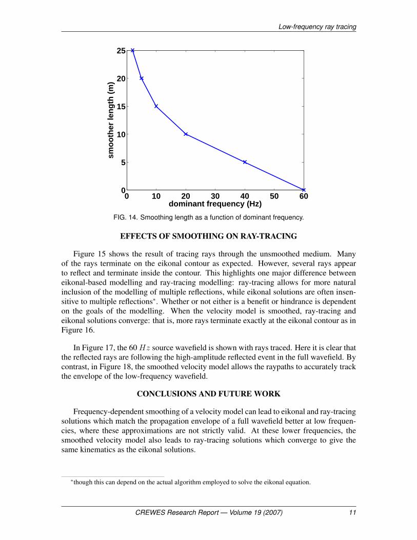
Next, lower-frequency finite-difference wavefields were calculated over the same un-smoothed medium. At the extreme low-frequency end (2 Hz dominant minimum phasesource), the outermost envelope of the wavefield coincides best with an eikonal solutionover the original velocity model smoothed by convolving with a Gaussian smoother withσ=25m, ie a smoothing length of 25m. For comparison, Figure 9 shows eikonal solutionsfor both unsmoothed and smoothed velocity models overlaid on the finite-difference solu-tion with a 2 Hz dominant source. At approximately (500, 800) on Figure 9, it may beseen that the smoothed-model eikonal contour extends farther down in the section than theamplitude of the original wavefield. This may be explained by considering the velocitymodel in Figure 6. The 25m smoother smears the high-velocity band between 800m and900m depth up into the low-velocity band between 700m and 800m. Thus the eikonal con-tour locally out-paces the actual velocity of propagation in this direction. This is purelya local effect, and is corrected upon farther propagation. Similar smoothed-model eikonalsolutions are overlaid on finite-difference solutions for a 5 Hz dominant source (Figure10), 10 Hz dominant source (Figure 11), 20 Hz dominant source (Figure 12), and a 40 Hzdominant source (Figure 13).

Overall results are summarized in Figure 14. At high frequency, the eikonal solutionsmatch the finite difference wavefield well. At lower frequencies, smoothing lengths up toσ =25m become necessary.

6 CREWES Research Report — Volume 19 (2007)

Low-frequency ray tracing

FIG. 6. Vertical sections of the velocity models used for eikonal solutions. On the left is the un-smoothed velocity model, on the right is the most heavily smoothed model.

FIG. 7. 60 Hz dominant source in unsmoothed velocity model, with eikonal solution to the un-smoothed model overlaid in blue.

CREWES Research Report — Volume 19 (2007) 7

Hogan and Margrave

FIG. 8. 2 Hz dominant source, with eikonal solution to the 25 m smoothing length model overlaid inblue.

FIG. 9. 2 Hz dominant source, 25 m smoothing length eikonal solution in white, unsmoothed velocitymodel eikonal solution in blue.

8 CREWES Research Report — Volume 19 (2007)

Low-frequency ray tracing

FIG. 10. 5 Hz dominant source, eikonal solution to 20 m smoothing length model overlaid in blue.

FIG. 11. 10 Hz dominant source, eikonal solution to 15 m smoothing length model overlaid in blue.

CREWES Research Report — Volume 19 (2007) 9

Hogan and Margrave

FIG. 12. 20 Hz dominant source, eikonal solution to 10 m smoothing length model overlaid in blue.

FIG. 13. 40 Hz dominant source, eikonal solution to 5 m smoothing length model overlaid in blue.

10 CREWES Research Report — Volume 19 (2007)

Low-frequency ray tracing

0 10 20 30 40 50 600

5

10

15

20

25

dominant frequency (Hz)

smo

oth

er le

ng

th (

m)

FIG. 14. Smoothing length as a function of dominant frequency.

EFFECTS OF SMOOTHING ON RAY-TRACING

Figure 15 shows the result of tracing rays through the unsmoothed medium. Manyof the rays terminate on the eikonal contour as expected. However, several rays appearto reflect and terminate inside the contour. This highlights one major difference betweeneikonal-based modelling and ray-tracing modelling: ray-tracing allows for more naturalinclusion of the modelling of multiple reflections, while eikonal solutions are often insen-sitive to multiple reflections∗. Whether or not either is a benefit or hindrance is dependenton the goals of the modelling. When the velocity model is smoothed, ray-tracing andeikonal solutions converge: that is, more rays terminate exactly at the eikonal contour as inFigure 16.

In Figure 17, the 60 Hz source wavefield is shown with rays traced. Here it is clear thatthe reflected rays are following the high-amplitude reflected event in the full wavefield. Bycontrast, in Figure 18, the smoothed velocity model allows the raypaths to accurately trackthe envelope of the low-frequency wavefield.

CONCLUSIONS AND FUTURE WORK

Frequency-dependent smoothing of a velocity model can lead to eikonal and ray-tracingsolutions which match the propagation envelope of a full wavefield better at low frequen-cies, where these approximations are not strictly valid. At these lower frequencies, thesmoothed velocity model also leads to ray-tracing solutions which converge to give thesame kinematics as the eikonal solutions.

∗though this can depend on the actual algorithm employed to solve the eikonal equation.

CREWES Research Report — Volume 19 (2007) 11

Hogan and Margrave

m

m

0 200 400 600 800 1000

0

200

400

600

800

1000

FIG. 15. Ray-tracing through the unsmoothed velocity model, with eikonal contour.

0 200 400 600 800 1000

0

200

400

600

800

1000

m

m

FIG. 16. Ray-tracing through the 25m smoothed velocity model, with eikonal contour.

12 CREWES Research Report — Volume 19 (2007)

Low-frequency ray tracing

0 200 400 600 800 1000

0

200

400

600

800

1000

m

m

FIG. 17. Ray-tracing through the unsmoothed velocity model, with 60 Hz dominant finite differencewavefield.

m

m

0 200 400 600 800 1000

0

200

400

600

800

1000

FIG. 18. Ray-tracing through the 25m smoothed velocity model, with 2 Hz dominant finite differencewavefield.

CREWES Research Report — Volume 19 (2007) 13

Hogan and Margrave

In the future, we will continue to investigate the full behaviour of these high-frequencyapproximations at low frequencies. We are currently working towards analytical approachesto determine optimal smoothing length. Additionally, we are considering alternative scale-dependent representations of given velocity models that may be more effective than a sim-ple frequency-dependent smoothing. Specifically, we are looking at extensive lineariza-tions of the hypereikonal equation that may allow for simple but theoretically-justifiablefrequency-dependent velocity models.

REFERENCES

Biondi, B., 1997, Solving the frequency-dependent eikonal equation, Tech. Rep. 73, Stanford ExplorationProject.

Hogan, C. M., and Margrave, G. F., 2006, Frequency-dependent velocity smoothing in GPSPI migration,Tech. rep., CREWES Research Report.

Margrave, G. F., and Ferguson, R. J., 1999, Wavefield extrapolation by nonstationary phase shift: Geophysics,64, 1067–1078.

Pujol, J., 2003, Elastic wave propagation and generation in seismology: Cambridge University Press.

Woodward, M. J., 1992, Wave-equation tomography: Geophysics, 57, No. 1, 15–26.

14 CREWES Research Report — Volume 19 (2007)