
rational pricing of internet companies revisited
31
RATIONAL PRICING OF INTERNET COMPANIES REVISITED* September 2000 Revised June 2001 Eduardo S. Schwartz Anderson School at UCLA Mark Moon Fuller & Thaler Asset Management *We thank Michael Brennan, Stephen Figlewski, Jun Liu, Steven Posner and seminar participants at Harvard, Princeton, Carnegie Mellon and Arizona for helpful comments and suggestions.
Transcript of rational pricing of internet companies revisited

RATIONAL PRICING OF INTERNET COMPANIES
REVISITED*
September 2000
Revised June 2001
Eduardo S. Schwartz
Anderson School at UCLA
Mark Moon
Fuller & Thaler Asset Management
*We thank Michael Brennan, Stephen Figlewski, Jun Liu, Steven Posner and seminar
participants at Harvard, Princeton, Carnegie Mellon and Arizona for helpful comments
and suggestions.

2
RATIONAL PRICING OF INTERNET COMPANIES REVISITED
Eduardo S. Schwartz and Mark Moon
Abstract
In this article we expand and improve the Internet company valuation model ofSchwartz and Moon (2000) in numerous ways. By using techniques from real optionstheory and modern capital budgeting, the earlier paper demonstrated that uncertaintyabout key variables plays a major role in the valuation of high growth Internetcompanies. Presently, we make the model more realistic by providing for stochasticcosts and future financing, and also by including capital expenditures and depreciation inthe analysis.
Perhaps more importantly, we offer insights into the practical implementation themodel. An important challenge to implementing the original model was estimating thevarious parameters of the model. Here, we improve the procedure by setting the speed ofadjustment parameters equal to one another, by tying the implied half-life of the revenuegrowth process to analyst forecasts, and by inferring the risk-adjustment parameter fromthe observed beta of the company’s stock price. We illustrate these extensions in avaluation of the company eBay.

3
RATONAL PRICING OF INTERNET COMPANIES REVISITED
1. INTRODUCTION
In Schwartz and Moon (2000) we develop a model for pricing Internet companies
using real options theory and modern capital budgeting techniques. The novelty of the
approach is that uncertainty about the key variables which determine the value of an
Internet company play a central role in the valuation. In particular, we consider
uncertainty in both the revenues and the rates of growth in revenues.
In this article we expand and improve the model in several directions. First, we
introduce a third stochastic variable to the model, variable costs. These are allowed to
follow a mean reverting process with volatility that also mean reverts deterministically.
This feature is important since many Internet companies have not yet been profitable but,
presumably, are expected to be profitable in the future.
Second, we use the fact that the theoretical framework allows us to compute the
“beta” of the stock as means of inferring the risk premium in the model. The estimation
of the market price of risk in the model, an unobservable parameter, was one of the most
challenging aspects of the approach. We can now use the beta of the Internet stock to
infer this parameter.
Third, we explicitly take into account capital expenditures and depreciation when
calculating the net after tax cash flows. This is done by introducing a third deterministic
path-dependant state variable – Property, Plant and Equipment – which increases with
capital expenditures and decreases with depreciation. This feature of the model is
important for Internet companies that require large investment in fixed assets.

4
Fourth, we attempt to improve the bankruptcy condition in the model by allowing
the cash balances to become negative. This provides for future equity and debt financing,
or for the possible future sale of the company. The optimal financing is that which
maximizes the value of the firm.
Fifth, we suggest a number of simplifying assumptions that considerably facilitate
the practical implementation of the model. One of these is to set all the speeds of
adjustment in the model equal to one another and derive them from the “half-life” of the
company to becoming a “normal” firm. Another simplification is to assume that both the
growth rates in revenues and variable costs are orthogonal to the “market” returns. Then,
only the revenue process has a risk premium associated with it, which must be estimated
to implement the model.
Sixth, we relate the half-life of the deviations to analysts’ (or the evaluator’s)
expectations about future revenues. This is done in recognition of the fact that the speed
of adjustment of the growth rate of revenues is critically important for valuation
purposes.
Seventh, when the market prices of the straight debt issues are available we use
them in the process of computing the value of the stock starting from the total value of
the firm.
The expanded model, then, has six state variables, three of which are stochastic
and three of which are deterministic (although path-dependant). The three stochastic
variables are the revenues, the growth rate in revenues and the variable costs. The three
deterministic path-dependant variables are the amount of cash available, the loss-carry-
forward and the accumulated Property, Plant and Equipment. We solve the problem by
5
Monte Carlo simulation which can easily deal with this number of state variables and the
complex path-dependencies of the problem.
In Section 2 we present the model with all the new features described above in its
continuous-time version. Since the model is solved by simulation using an interval of
time that can be quite long, such as one quarter or one year, Section 3 discusses in detail a
discrete time approximation. Section 4 provides an illustrative example of the approach
by pricing eBay stock and Section 5 presents comparative statics with respect to some of
the key parameters. Section 6 concludes.
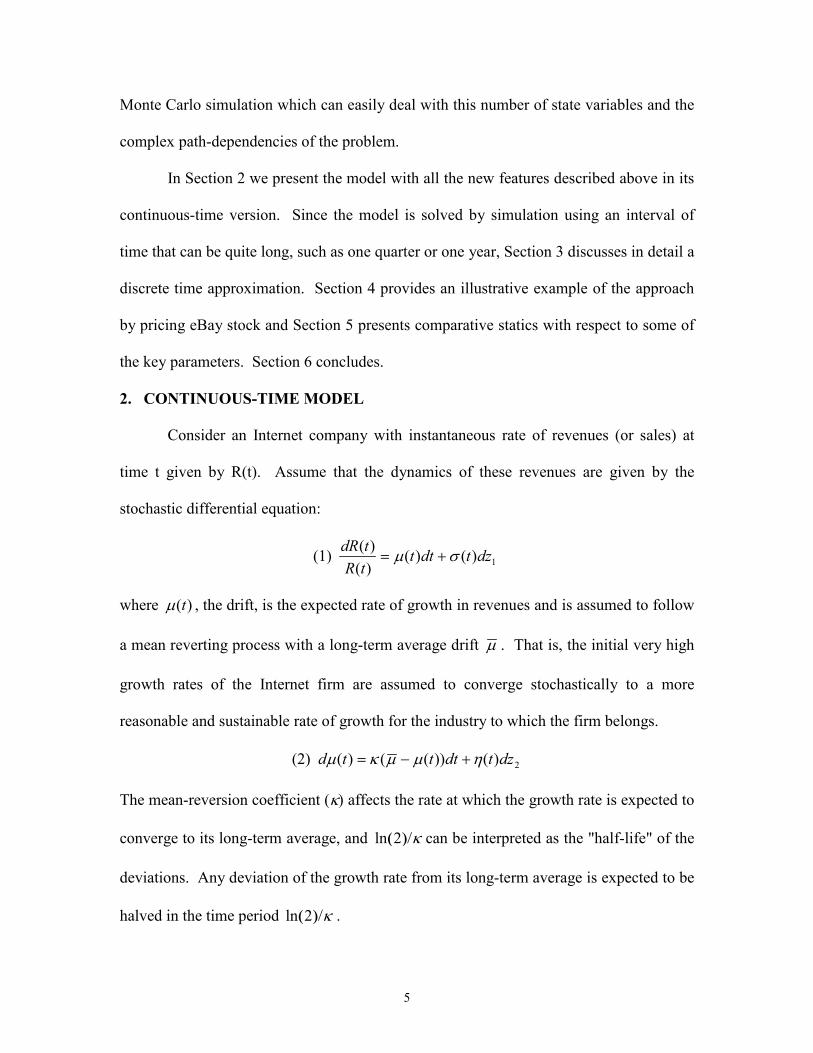
2. CONTINUOUS-TIME MODEL
Consider an Internet company with instantaneous rate of revenues (or sales) at
time t given by R(t). Assume that the dynamics of these revenues are given by the
stochastic differential equation:
(1) 1)()()()( dztdtt
tRtdR
�� ��
where )(t� , the drift, is the expected rate of growth in revenues and is assumed to follow
a mean reverting process with a long-term average drift � . That is, the initial very high
growth rates of the Internet firm are assumed to converge stochastically to a more
reasonable and sustainable rate of growth for the industry to which the firm belongs.
(2) 2)())(()( dztdtttd ����� ���
The mean-reversion coefficient (�) affects the rate at which the growth rate is expected to
converge to its long-term average, and ����2ln can be interpreted as the "half-life" of the
deviations. Any deviation of the growth rate from its long-term average is expected to be
halved in the time period ����2ln �

6
The unanticipated changes in revenues are also assumed to converge
(deterministically) to a more normal level whereas the unanticipated changes in the
expected growth rate are assumed to converge (also deterministically) to zero.
(3) dtttd ))(()( 1 ���� ��
(4) dtttd )()( 2��� ��
The unanticipated changes in the growth rate of revenues and the unanticipated changes
in its drift may be correlated:
(5) dtdzdz 1221 ��
Total costs at time any t have two components.1 The first is a variable
component, which is assumed to be proportional to the revenues. The second is a fixed
component.
(6) FtRttCost �� )()()( �
The variable costs parameter �(t) in the cost function is also assumed to be
stochastic reflecting the uncertainty about future potential competitors, market share, and
technological developments. It follows the stochastic differential equation:
(7) 33 )())(()( dztdtttd ����� ���
The mean-reversion coefficient (��) describes the rate at which the variable costs are
expected to converge to their long-term average, and 32ln ���� can be interpreted as the
"half-life" of the deviations. Any deviation of the variable costs from its long-term
average is expected to be halved in this time period. The unanticipated changes in
variable costs are also assumed to converge (deterministically) to a more normal level
1 More complicated cost functions can easily be incorporated in the analysis since the problem is solved bysimulation.

7
(8) dtttd ))(()( 4 ���� ��
We also allow for correlation between unanticipated changes in variable costs and
both revenues and growth rates in revenues:
(9) dtdzdz 1331 �� (10) dtdzdz 2332 ��
The after tax rate of net income to the firm, Y(t), is then given by
(11) )1))(()()(()( ctDeptCosttRtY �����
The corporate tax rate �c in (11) is only paid if there is no accumulated loss-carry-
forward (i.e. if the loss-carry-forward is positive the tax rate is zero) and the net income is
positive. The dynamics of the loss-carry-forward are given by:
(12) dL(t) = - Y(t)dt if L(t) > 0
dL(t) = Max [- Y(t)dt , 0] if L(t) = 0
The accumulated Property, Plant and Equipment at time t, P(t), depends on the
rate of capital expenditures for the period, Capx(t), and the corresponding rate of
depreciation, Dep(t). Planned capital expenditures, CX(t), are known for an initial
period and after that they are assumed to be a fraction CR of revenues. Depreciation is
assumed to be a fraction DR of the accumulated Property, Plant and Equipment.
(13) dttDeptCapxtdP )}()({)( ��
(14) ttfortCXtCapx �� )()(
ttfortRCRtCapx �� )(*)(
(15) )(*)( tPDRtDep �
Then, the amount of cash available to the firm, given by X(t), evolves according
to:

8
(16) dttCapxtDeptYtrXtdX )}()()()({)( ����
The untaxed interest earned on the cash available is included in the dynamics of the cash
available to make the valuation results insensitive to when the cash flows are distributed
to the security-holders. Since in the risk neutral framework we discount risk adjusted
cash flows at the risk free rate of interest, we also need to accumulate cash flows at the
same risk free rate. For all purposes, except for determining the bankruptcy condition,
this is equivalent to discounting the cash flows generated by the firm when they occur as
opposed to at the horizon T.
To avoid having to define a dividend policy in the model, we assume that the cash
flow generated by the firm’s operations remains in the firm and earns the risk free rate of
interest. This accumulated cash will be available for distribution to the shareholders at an
arbitrary long-term horizon T, by which time the firm will have reverted to a “normal”
firm.
The firm is assumed to go bankrupt when its cash available reaches a
predetermined negative amount, X*. The purpose of this is to allow for future financing.
The optimal amount of new financing in the future is the one which maximizes the
current value of the firm, though we recognize that in many practical situations firms go
bankrupt before their value reaches zero. To obtain the “optimal” amount of new
financing we decrease X* until firm value is maximized. The true optimal amount of new
financing, however, is state-dependant and has to be obtained jointly with the valuation
of the firm using dynamic programming type techniques. Longstaff and Schwartz (2001)
show how to solve this problem using cross-sectional information from the simulation in
least-squares regressions.

9
The objective of the model is to determine the value of the Internet firm at the
current time. According to standard theory this value is obtained by discounting the
expected value of the firm at the horizon under the risk neutral measure (the equivalent
martingale measure) at the risk free rate of interest, which for simplicity is assumed to be
constant2. The value of the firm at the horizon T has two components. First, the cash
balance outstanding and second, the value of the firm as a going concern which is
assumed to be a multiple M of the EBITDA at the horizon T:
(17) rTQ eTCostTRMTXEV �
���� )]}()([)({)0(
The model has three sources of uncertainty. First, there is uncertainty about the
changes in revenues, second, there is uncertainty about the expected rate of growth in
revenues and third, there is uncertainty about the variable costs. We will assume that only
the first source of uncertainty has a risk premium associated with it and later on we will
relate this risk premium to the “beta” of the stock. Under some simplifying assumptions
leading to the Intertemporal Capital Asset Pricing Model of Merton (1973) the risk
adjusted processes for revenues can be obtained from the true processes as in:
(18) *1)()]()([
)()( dztdttt
tRtdR
��� ���
where the risk premium � (t) is related to the covariance between the revenue process
and the return on the market portfolio. Since the processes for the growth rate of
revenues and variable costs do not have risk premiums associated with them, the true and
the risk-adjusted processes are the same.
Most analysts and investors are more interested in the price of a share than in the
value of a whole company. To obtain the price of a share from the total value of the firm
2 It would be easy to incorporate stochastic interest rates into our framework.
10
we need to examine the capital structure of the company in detail. We need to know how
many shares are currently outstanding and how many shares are likely to be issued to
current employee stock option holders and convertible bondholders. We also need to
know how much of the cash flows will be available to the shareholders after coupon and
principal payments to the bondholders.
To simplify the analysis, we assume that if the firm survives options will be
exercised and convertible bonds will be converted into shares.3 This means that in each
of the paths of the simulation where the company does not go bankrupt, we adjust the
number of shares to reflect the exercise of options and convertibles. To obtain the cash
flows available to shareholders from the cash flows available to all security-holders
(which determine the total value of the firm), we subtract the principal and after-tax
coupon payments on the debt4 and add the payments by option holders at the exercise of
the options. Since we are assuming that the firm pays no dividends, the exercise of the
options and convertibles occurs at their maturity. If all option holders exercise their
options optimally, the above procedure overvalues the stock by undervaluing the options
and convertibles, since there might be some states of the world where the firm survives
but it is not optimal to exercise the options or convert the convertibles.
In addition, it is well known, that for diversification purposes, employee stock
options are frequently exercised before maturity, if they are exercisable, to allow for the
sale of the underlying stock. Also, even if they are in the money, not all of the options
will be exercised since many of the employees will leave the firm before their options
vest. However, over time the firm will likely issue additional employee stock options to
3 The Longstaff and Schwartz (2001) approach could be used to obtain a more precise exercise strategy.4 When the market price of bonds is available we subtract it directly from the firm value.
11
existing and new employees. If the number of shares to be issued at exercise and
conversion is small relative to the total number of shares outstanding, the impact of these
issues on the share value is likely to be very small.
Implicit in the model described above is that the value of the firm and the value of
the stock at any point in time are functions of the value of the state variables (revenues,
expected growth in revenues, variable costs, loss-carry-forward, cash balances and
accumulated Property, Plant and Equipment) and time. That is, the value of the stock can
be written as:
(18) ),,,,,,( tPXLRSS ���
Applying Ito’s Lemma to this expression we can obtain the dynamics of the stock value
(19) ������
��
��������
��
ddSdRdSdRdSdSdS
dRSdtSdPSdXSdLSdSdSdRSdS
RR
RRtPXLR
����
���������
2212
21
221
The volatility of the stock can be derived directly from this expression
(20) 2313122222
222 222)()()( �������������������
S
VS
S
SS
S
SSSS
SS
SS
S RRR RRR������
The partial derivatives of the stock value with respect to the level of revenues, to
the expected rate of growth in revenues, and to the variable costs are obtained by
simulation5. Since the initial volatility of the expected growth rate of revenues (�0) is one
of the most critical parameters in the valuation model and is difficult to estimate,
equation (20) is used in the implementation of the model to imply �0 from the observed
volatility of the stock price.
5 The initial value of the revenues (the rate of growth in revenues and the variable costs) is perturbed toobtain new values of the equity from which these derivatives are computed.

12
Using expression (19) and the continuous time return on the market portfolio, and
noting that only the revenue process is correlated with the return on the market, we can
write the “beta” of the stock as a function of the “beta” of the revenues:
(21) RR
M
MRMR
M
SMS S
RStS
RS�
�
���
�
�� ��� 22
)(
From the Intertemporal Capital Asset Pricing Model we can write the expected
return on the stock as:
(22) )()( rrS
RSrrrrr MRR
MSS ������ ��
By equating the expected return on the stock given by (22) with the one obtained
from (19) we can derive the risk premium in the model, �(t):
(23) )()( rrt MR �� ��
Finally, using (21) and (23) we can write the beta of the stock as a function of the
risk premium in the model:
(24) rr
tS
RS
M
RS
�
�
)(��
We can then use (24) to infer the risk premium from the beta of the stock. In the
implementation of the model we set )()( tt ��� � since the volatility of the revenues
changes with time and the risk premium is proportional to the beta of the revenues.
3. DISCRETE-TIME APPROXIMATION OF THE MODEL
The model developed in the previous section is path-dependent. The cash
available at any point in time, which determines when bankruptcy is triggered, depends
on the whole history of past cash flows. Similarly, the loss-carry-forward and the
depreciation tax shields, which determine the timing and amount of corporate taxes the

13
firm has to pay, are also path-dependent. These path-dependencies can easily be taken
into account by using Monte Carlo simulation to solve for the value of the Internet
company.
In the implementation of the model we assume that all the mean reversion
coefficients are equal and their unique value is inferred from the expected half-life of the
deviations in growth rates in revenues. To perform the simulation we use the discrete
version of the risk-adjusted processes:6
(25) })(]
2)(
)()({[ 1
2
)()(��
���� ttt
ttt
etRttR�����
���
(26) 2
2
)(2
1)1()()( ���
���
�
�� teetettt
tt��
���� �������
(27) 3
2
)(2
1)1()()( ���
���
�
�� teetettt
tt��
���� �������
where
(28) )1()( 0tt eet ��
�����
���
(29) tet �
���
� 0)(
(30) )1()( 0tt eet ��
�����
���
Equations (28) - (30) are obtained by integrating (3), (4) and (8) with initial values 0� ,
0� and 0� . These are exact solutions, not approximations. 1� , 2� and 3� are standard
correlated normal variates.
6 Note that there is a typo in the equation corresponding to (26) in Schwartz and Moon (2000).
14
The mean reverting processes for the rate of growth in revenues (Equation (2))
and for the variable costs (Equation (7)) with their respective volatilities decreasing with
time according to (29) and (30) allow for a closed form solution for the future distribution
of these variables. For example, the variable costs at time t are normally distributed with
mean and variance equal to:
(31) )1()]([ 0tt eetE ��
�����
���
(32)�
��
��������
��
��
211)(2)2()]([
222
022
020
tttt eeetetVar
��
���
��
�����
where for simplicity we have assumed that the mean reversion parameter in the variable
cost process and its volatility are the same.
In the limit when t goes to infinity this distribution converges to a normal with
mean and variance:
(33) �� ��)]([E
(34)�
��
2)]([
2
��Var
The distribution of the growth rate of revenues is equivalent, but with the long-
term volatility equal to zero.
Note that as time grows the volatilities in the model converge to:
(35) �� ��)(
(36) 0)( ���
(37) �� ��)(
and the growth rate of revenues converges to
(38) �� ��)(
15
This implies that the revenue process converges to
(39) 1)()( dzdt
RdR
�� ��
�
�
The net income after tax is still given by equation (11) where all variables are
measured over the period t� . Similarly, the discrete versions of the dynamics of the
loss-carry-forward, the accumulated Property, Plant and Equipment, and the amount of
cash available are immediate.
Depending on the situation, the unit of time t� chosen for the analysis is one quarter
or one year. The advantage of using the latter is that it allows for smoothing of seasonal
effects and is more consistent with typically annual longer-term analyst projections.
4. ILLUSTRATIVE EXAMPLE
In this section we apply the model described in previous sections to value eBay.
Ebay is the world’s largest online trading community. Founded in September 1995, it is
a marketplace for the sale of goods and services by a community of individuals and small
businesses. At the beginning of the year 2001 it included 18.9 million registered users.
The results obtained from our valuation approach, like those of any other valuation
approach, depend critically on the assumptions we make about future revenues, rates of
growth in revenues, and costs. In what follows we describe how we estimate the
parameters needed to run the Monte Carlo simulation from the past and present data
available for eBay, and from analysts forecasts relating to the company. Since most
forecasts of capital expenditures, revenues and costs are available on an annual basis, all
of our simulations are done on an annual basis.

16
Revenue Dynamics
As the starting value for the revenue simulation we take the actual revenues for
2000 of $431 million. The initial volatility of revenues is obtained from quarterly data
from the third quarter of 1998 to the fourth quarter of 2000, and annualized to give 0.167.
This volatility is assumed to decrease with time to the long-term volatility of revenues of
0.0837. The half-life of this deviation and of all the others in the model are assumed to be
2.8 years. Later on we explain in more detail how we obtain this value for the half-life.
Growth Rate of Revenues Dynamics
The initial growth rate of revenues is taken to be 43.4% continuously
compounded per year. This represents the average forecast of four analysts for the growth
rate from 2000 to 2001. It is assumed that in the long run, when eBay becomes a
“normal” firm, this growth rate will decrease to 5% per year. The initial annual volatility
of the growth rate, which is one of the critical parameters in the model, is unobservable.
We imply it from the volatility of the stock. Figure 1 shows the daily implied volatility
of eBay options from February 1, 1999 to March 30, 2001. The average implied
volatility of the stock during this period was 91%.
Figure 2 shows distributions of the rate of growth in revenues implied from these
parameters in one, three and ten years. Note that the distribution shrinks and moves left
as time increases; it converges to a constant 0.05 at infinity.
Variable Cost Dynamics
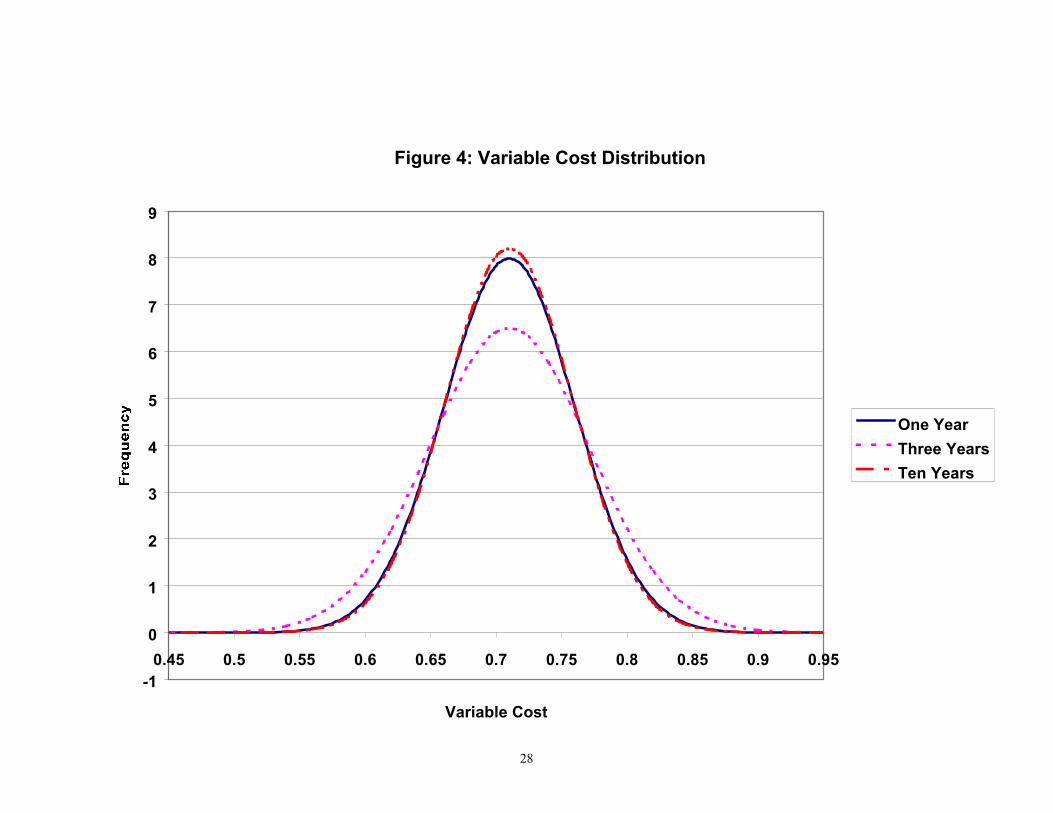
Using actual data for 1999 and 2000, and analyst estimates for 2001, Figure 3
reports the results of regressing cash costs on revenues. From these results we take 0.71
as the initial variable cost as a fraction of revenues, and $43 million as the annual fixed

17
cost. We assume that in the long run variable costs will remain at $0.71 per dollar of
revenue. Finally, we assume that the initial volatility of variable costs of 0.06 will
decrease in the long run to 0.03. With these assumptions the distributions of variable
costs one year, three years and ten years in the future are shown in Figure 4. The mean of
the distribution remains at 0.71, but note that the standard deviation first increases from
one to three years and then decreases from three to ten years.
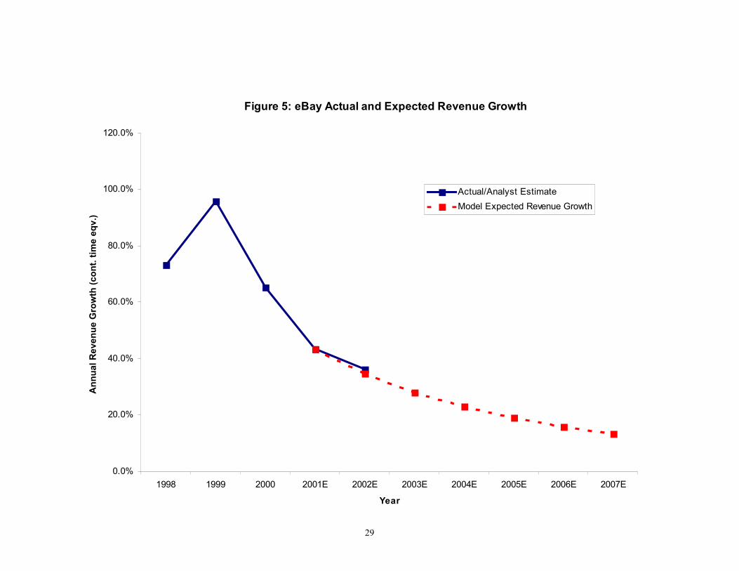
Half-Life of Deviations and Correlations
As mentioned earlier, to simplify the analysis we have assumed that all the mean
reversion processes in the model have the same speed of adjustment coefficient. The
mean reversion parameter that determines how fast the initial growth rate of revenues
reverts to its long-term rate has the most significant effect on valuation. This is not
surprising. If we start with an initial growth rate of 43.4% and we assume that in the long
run it decreases to a more normal 5%, then the speed at which it decreases will have a
tremendous impact on future revenues. Figure 5 shows the actual and expected growth
rate of revenues predicted by analysts and implied by the model parameters. Note that
with a half-life of 2.8 years, the model expected revenue growth closely matches the
analysts revenue growth prediction for 2002.
In this illustration we have assumed that the three stochastic processes are
uncorrelated. In the next section we consider the effect of possible correlations between
the variables.
Balance Sheet Data
7 The valuation results are not sensitive to this parameter.
18
The cash and marketable securities available at the end of the year 2000 was $556
million and the firm had no loss-carry-forward at that point in time. The accumulated
property, plan and equipment was $125.2 million.
The number of shares outstanding was 269.311 million shares. In addition the
company had 26.249 million employee stock options outstanding with a weighted-
average life of 8.4 years and a weighted average exercise price of $38.99.8 Finally, the
firm had only $27 million of mortgage debt outstanding9. This information is used to
determine the price of the stock starting from the total value of the firm.
Capital Expenditures and Depreciation
Analysts have forecasted eBay’s capital expenditures to be $64 million, 13% of
revenues, in the year 2001. So, starting from 2002 we assume that capital expenditures
will be 13% of revenues. In accordance with the firm practice we assume that the annual
depreciation allowance is 33% of the accumulated property, plant and equipment of the
previous year.
Environmental and Risk Parameters
The corporate tax rate is taken to be 35% and the risk free rate of interest 5%.
The risk premium on the market portfolio used in the model to relate the market price of
risk to the beta of the stock is assumed to be 6%.
The market price of risk in the model corresponding to the revenue process is an
unobservable parameter. We imply it from the beta of the stock. Figure 6 shows the
regression used to estimate beta using weekly stock returns for eBay and the S&P 500
8 The computer program actually uses the more detailed employee stock options data.9 Since the amount of debt outstanding was so minimal, it was subtracted from the cash and marketablesecurities outstanding. We then assumed that eBay had no debt in its capital structure.
19
Index from September 25, 1998 to March 30, 2001.10 The estimated beta is 2.67. In the
calculations, however, we use the Bloomberg adjusted beta of 1.76 to take into account
measurement error in the estimation of beta and the fact that in the ten year horizon
considered the beta will tend to revert to 1.
Simulation Parameters
In all cases we use 10,000 simulations with steps of one year and up to a horizon
of 10 years. At the horizon we assume that the terminal value of the firm is a multiple of
ten times earnings before interest, taxes, depreciation and amortization (EBITDA).
Simulation Results
Using the parameters described above, the model stock price for eBay that we
obtain is $22.41, with model volatility and beta that closely match (by construction)
observed volatility and beta of the stock. The model (risk neutral) probability of
bankruptcy is very small (less than 0.1%).
On April 11, 2001 the market price of eBay at the close was $39.17. This is 75%
above the model price!
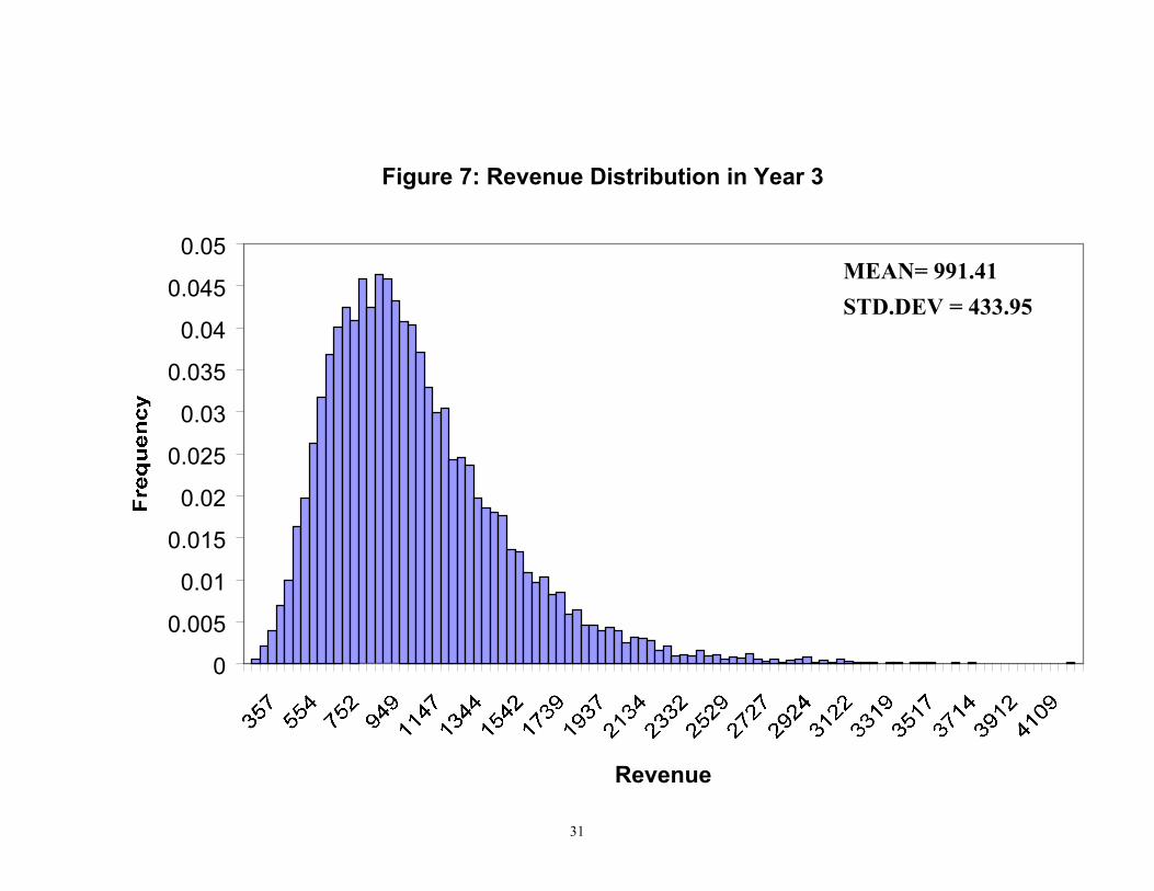
Figure 7 shows the (risk neutral) frequency distribution of revenues at the end of
year 3 implied by the above parameters. As can be seen from the figure there is
substantial uncertainty about the revenues in the model even three years in the future.
(Note that with only 10,000 simulations the frequency distribution does not appear as
smooth as it really is.)
NPV Results
10 A more detailed analysis would probably use a broader market index for this calculation.
20
By setting all the volatilities in the model equal to zero we can obtain the Net
Present Value of the cash flows using exactly the same data as in the previous analysis.11
The only additional parameter we need is the risk-adjusted discount rate. Taking into
account that eBay is an all equity financed firm we use the same parameters for the risk
free rate, the risk premium on the market and the beta of the stock to infer the required
return on equity using the CAPM. The resulting discount rate is 16% and the
corresponding stock value is $11.11.
There is a difference of $11.30 ($22.41-$11.11) between the model price and the
NPV price using exactly the same data. The only parameters not used in the NPV
calculation are the volatilities and correlations. There are two sources for this difference,
both of which are introduced by including in the analysis the whole distributions of the
state variables. The first source of value is the abandonment option that allows the firm
to exit through bankruptcy if outcomes are very poor. The second source of value can be
explained by Jensen’s inequality, which shows that the expected value of a non-linear
convex function of several variables is greater than the function of the expected values of
those variables. This second source of value has not been generally recognized in the real
options literature. In our specific example it is the dominant effect since the probability
of bankruptcy is very small.
5. SENSITIVITY ANALYSIS
In this section we perform some sensitivity analysis on the more critical or
controversial parameters of the model.
Correlations
11 We only need to run one simulation since all of them will be the same in this case.
21
Consider the situation in which the firm is in a competitive environment such that
increases in profit margins (i.e. decreases in variable costs) are associated with decreases
in growth rates in revenues. This implies a positive correlation between variable costs
and growth rates in revenues. We run the program with the same data described above,
but assuming a correlation of 0.5. The market price of risk and the volatility of the
growth rate had to be adjusted slightly to match the volatility and the beta of the stock.
The model price decreased only slightly to $21.89. The effect of this correlation on
prices increases, however, with the volatility of variable costs.
Variable Costs
As expected, long-term variable costs have a big effect on prices. If long-term
variable costs are increased from 0.71 to 0.74, the model stock price goes down to $20.61
and if they are decreased to 0.68, the model stock price goes up to $24.51. In both cases
small adjustments are needed in the market price of risk to match the beta of the stock.
This result is not surprising: a 10% increase or decrease in the profit margin has a similar
effect on model stock prices.
Half-Life of Deviations
The speed of adjustment has an important impact on expected future revenues and
therefore on valuation since it determines how fast the growth rate ofrevenues (and the
other variables) will decrease. If we increase the half-life parameter from 2.8 to 3.0
years, the stock price increases to $24.20. If we decrease the parameter to 2.6 years the
stock price decreases to $20.65.
Horizon and Terminal Value
22
In the illustration we are exploring an increase in the horizon of the simulations
from 10 to 11 years has no effect on the model value of the share. It changes the share
price to $22.65 which is well within the standard error of the simulation. An increase in
the multiple of earnings used to determine the terminal value of the stock, however, has a
significant effect on the share value. An increase of this multiple from 10 to 11, increases
the share value to $23.84.
6. CONCLUSION
In this article we substantially extend the model developed in Schwartz and Moon
(2000) for pricing Internet companies. We introduce uncertainty in costs and we take
into account the tax effects of depreciation. We use the beta and the volatility of the
stock to infer two critical unobservable parameters of the model, the market price of risk
and the volatility of growth rates in revenues. We improve the bankruptcy condition by
allowing future financing by the firm. Finally, we facilitate the implementation of the
model by assuming the half-life of all processes is the same and suggest that it can be
estimated from evaluator’s expectations of future revenues.
An interesting and important issue that has not been explored in this article is the
use of the probabilities of bankruptcy obtained from the model to infer the credit rating of
the firm. Alternatively, the credit ratings of the firm could be used to better estimate some
of the unobservable parameters of the model, in a similar manner as the beta and the
volatility of the stock are used to infer the risk parameter in the model and the volatility
of the growth rate of revenues, respectively.
The discussion in this article has concentrated in the valuation of Internet stocks.
However, any high-growth stock can be analyzed using the techniques developed here.
23
Like any other valuation method, our real options approach to valuing Internet
companies depends critically on the parameters used in the estimation. The next step in
the implementation of the model would be to use cross-sectional data of many Internet
companies to estimate some of the parameters. Finally, since the growth rate of revenues
is not observable “learning models” could be used to update this critical factor in the
model when new information on revenues is revealed.

24
References
Longstaff, F.A. and E.S. Schwartz, (2001), “Valuing American Options by Simulation: A
Simple Least-Square Approach”, Review of Financial Studies 14:1, 113-147 (Spring).
Merton, R.C., (1973), “An Intertemporal Capital Asset Pricing Model”, Econometrica
41:4, 867-888 (February).
Schwartz, E.S. and M. Moon, (2000), “Rational Pricing of Internet Companies”,
Financial Analysts Journal 56:3, 62-75 (May/June).

Figure 1: eBay Daily Implied Volatility (%)February 1, 1999 to March 30, 2001
Average Volatility: 91%
0
20
40
60
80
100
120
140
160
31-Jan-99 1-May-99 30-Jul-99 28-Oct-99 26-Jan-00 25-Apr-00 24-Jul-00 22-Oct-00 20-Jan-01

26
Figure 2: Growth Rate of Revenues Distribution
0
1
2
3
4
5
6
-0.5 -0.3 -0.1 0.1 0.3 0.5 0.7 0.9
Growth Rate of Revenues
One YearThree YearsTen Years

27
Figure 3: eBay Cash Costs vs. RevenuesNot Including CAPX
1999A, 2000A, E[20001]
y = 0.7085x + 42.916R2 = 0.9994
0
100
200
300
400
500
600
0 100 200 300 400 500 600 700
Annual Revenues ($MM)
28
Figure 4: Variable Cost Distribution
-1
0
1
2
3
4
5
6
7
8
9
0.45 0.5 0.55 0.6 0.65 0.7 0.75 0.8 0.85 0.9 0.95
Variable Cost
One YearThree YearsTen Years
29
Figure 5: eBay Actual and Expected Revenue Growth
0.0%
20.0%
40.0%
60.0%
80.0%
100.0%
120.0%
1998 1999 2000 2001E 2002E 2003E 2004E 2005E 2006E 2007E
Year
Ann
ual R
even
ue G
row
th (c
ont.
time
eqv.
)
Actual/Analyst EstimateModel Expected Revenue Growth

30
Figure 6: eBay returns vs. S&P500 returnsWeekly data from September 25, 1998 to March 30, 2001
y = 2.667x + 0.0205R2 = 0.2246
-0.400
-0.300
-0.200
-0.100
0.000
0.100
0.200
0.300
0.400
0.500
-0.150 -0.100 -0.050 0.000 0.050 0.100 0.150
S&P500 Return
Bloomberg Beta 1.76
31
Figure 7: Revenue Distribution in Year 3
0
0.005
0.01
0.015
0.02
0.025
0.03
0.035
0.04
0.045
0.05
Revenue
MEAN= 991.41STD.DEV = 433.95