Economics 504Chris Georges Handout on Rational Expectations

Review of Statistics: Notation and Definitions

Consider two random variables X and Y defined over m distinct possible events. Event i occurs withprobability pi, in which case X and Y take on values xi and yi. Thus the probabilities of the variousevents occurring are p1, p2, ..., pm, and X and Y take on possible values x1, x2, ..., xm and y1, y2, ..., ym

respectively. If we have considered all possible events, then it must be that the sum of the m probabilitiesis one:

∑m

i=1 pi = 1.

For example, consider the following game. We flip a coin once. In the event that it lands heads-up, Bethand Bob each get $1. In the event the coin lands tails-up, Beth gets $2 and Bob gets nothing. Here thereare two possible events (heads and tails), which occur with equal probability p1 = p2 = 0.5. The payoffs toBeth and Bob are each random variables which we could call X and Y .

We will use the following notation

E(X) = The Expected Value of X

Var(X) = The Variance of X

Cov(X, Y ) = The Covariance of X and Y

µX = E(X)

σX = The Standard Deviation of X

ρXY = The Correlation of X and Y

These quantities are defined as follows.

E(X) = p1x1 + p2x2 + ... + pmxm

=

m∑

i=1

pixi

Var(X) = p1(x1 − µX)2 + p2(x2 − µX)2 + ... + pm(xm − µX)2

=

m∑

i=1

pi(xi − µX)2

= E[(X − µX)2]

σX =√

Var(X)

Cov(X, Y ) = p1(x1 − µX)(y1 − µY ) + p2(x2 − µX)(y2 − µY ) + ... + pm(xm − µX)(ym − µY )

=

m∑

i=1

pi(xi − µX)(yi − µY )

= E[(X − µx)(Y − µY )]

ρXY =Cov(X, Y )

σXσY

The expected value of X is an average or mean value of the realizations x which occur with frequenciesp. The variance of X is a measure of the average amount of variation of the realizations x around their meanvalue. The covariance of X and Y is a measure of the degree to which values of X which are larger thanaverage tend to coincide with values of Y which are larger or smaller than average. For example, a negative

1

covariance indicates that when the realization of X is greater than µX , the corresponding realization of Ytends, on average, to be less than µY . The correlation of X and Y is the covariance normalized so that thisvalue falls between −1 and 1. We say that X and Y are perfectly correlated if this correlation is −1 or 1.

Returning to our example of Beth and Bob, above, we have E(X) = $1.50, E(Y ) = $0.50, Var(X) =Var(Y ) = 0.25, σX = σY = 0.5, Cov(X, Y ) = −0.25, and ρXY = −1.

Review of Statistics: Identities

Let a, b, and c be arbitrary constants. The following identities follow from the definitions above.

E(a) = a

E(a + X) = a + E(X)

E(bX) = bE(X)

E(a + bX) = a + bE(X)

E(X + Y ) = E(X) + E(Y )

E(

n∑

i=1

Xi) =

n∑

i=1

E(Xi)

In the last identity, X1, X2, ... Xn are n random variables.

Var(a) = 0

Var(a + X) = Var(X)

Var(bX) = b2Var(X)

Var(X + Y ) = Var(X) + Var(Y ) + 2Cov(X, Y )

Var(

n∑

i=1

Xi) =

n∑

i=1

Var(Xi) +

n∑

i=1

n∑

j=1

j 6=i

Cov(Xi, Xj)

It follows from the last identity that if n random variables are mutually uncorrelated, the variance of theirsum is equal to the sum of their variances.

Cov(X, Y ) = Cov(Y, X)

Cov(X, X) = Var(X)

Cov(a, X) = 0

Cov(a + X, b + Y ) = Cov(X, Y )

Cov(bX, Y ) = bCov(X, Y )

Cov(bX, cY ) = bcCov(X, Y )

Cov(X, Y + Z) = Cov(X, Y ) + Cov(X, Z)

These identities can be proved easily by employing the definitions given above. For example, the identityE(a + X) = a + E(X) can be proved as follows:

2

E(a + X) =

m∑

i=1

pi(a + xi)

=

m∑

i=1

pia +

m∑

i=1

pixi

= (a

m∑

i=1

pi) + E(X)

= a + E(X)

Similarly, the identity Var(a + X) = Var(X) can be proved as follows:

Var(a + X) = E[((a + X) − E(a + X))2]

= E[((a −E(a)) + (X −E(X)))2 ]

= E[(X − E(X))2 ]

= Var(X)

Simple Application: Reducing Risk Through Diversification

We can show that the risk of the return on a financial portfolio can be reduced by diversification amonga large number of securities with risky but mutually uncorrelated returns.

Consider holding a portfolio of N securities with weights si (si is the proportion of the dollar value ofthe portfolio held in security i) and rates of return ri (ri is the rate of return per dollar held in security i).

For a portfolio of dollar value P , the rate of return on the portfolio is

rP =s1Pr1 + s2Pr2 + ... + sNPrN

P

=

N∑

i=1

siri

Each return ri is a random variable (i.e., individual security returns are risky), and consequently so is thereturn on the portfolio rP .

The expected rate of return on the portfolio is

E(rp) = E(

N∑

i=1

siri)

=N∑

i=1

siE(ri)

and if we measure the riskiness of the portfolio as the variance of its return, then this riskiness is

Var(rp) = Var(

N∑

i=1

siri)

= [

N∑

i=1

s2i Var(ri)] + [

N∑

i=1

N∑

j=1

j 6=i

sisjCov(ri, rj)]

3

Further, if the returns of the individual securities are mutually uncorrelated, then all the covariances aboveare zero, so that

Var(rp) =N∑

i=1

s2i Var(ri)

Now suppose that we hold equal shares of each security, so that si = 1/N ∀i, and for simplicity furthersuppose that the variance of each security’s returns is identical: Var(ri) = σ2 ∀i. Then for N independent(uncorrelated) securities

Var(rp) =

N∑

i=1

(1

N)2σ2

= N · (1

N)2σ2

=σ2

N

Thus, as we increase the number of independent securities held in the portfolio (i.e., increase the degreeof diversification of the portfolio), the portfolio’s riskiness becomes smaller and goes to zero in the limit asN → ∞. Intuitively, as the number of securities increases, the likelihood that the all do very well or all dovery poorly falls, and the likelihood that the realized portfolio return is near its expected value increases.

Note that positive covariances of returns across securities would limit our ability to reduce risk throughdiversification, and negative covariances would increase our ability to do this with a small number of secu-rities. Models of asset prices, such as CAPM, usually conclude that securities should only command riskpremia (extranormal expected returns) for non-diversifiable (also called ‘systematic’) risk. Thus, a securitymight have a highly uncertain return, but if its covariation with the rest of the market is small, it may havean expected return close to the rates on relatively riskless assets, since much of its risk can be diversifiedaway.

A central cause of the financial crisis of 2007-2008 was that various financial market participants (AIG,Bear Stearns, Countrywide, etc.) grossly underestimated the systematic risk that they were exposed to.For example, mortgage backed securities were rated and priced on the assumption that housing prices werehighly unlikely to fall and mortgage delinquencies rise nationwide so that packaging mortgages from differentregional markets was effectively diversifying away risk.

Expectations: Rational and Otherwise

The expectations of economic agents concerning the uncertain outcomes of future event often playimportant roles in determining market outcomes, both in the present and in the future. For example, thecurrent demand and supplies of oil, bonds, and other commodities depend on the expectations of their futureprices on the part of buyers and sellers in those markets. Thus, the current prices of these commodities dependon expectations of their future prices. Similarly, expectations of future economy-wide inflation can drive upthe demand for goods and credit today, causing inflation and interest rates to rise today, and expectationsof recession can lead to a fall in demand, creating a self fulfilling prophesy.

Rational Expectations

There are a variety of definitions of rational expectations in the economics literature. Intuitively, a ratio-nal expectation should be a best possible forecast based on all available information. We can operationalizethis by saying that the rational expectation should be a mathematical expectation (expected value). Call

Xe(t)t+j the expectation at time t of the future random variable Xt+j . Then if expectations are rational,

Xe(t)t+j = EtXt+j

4

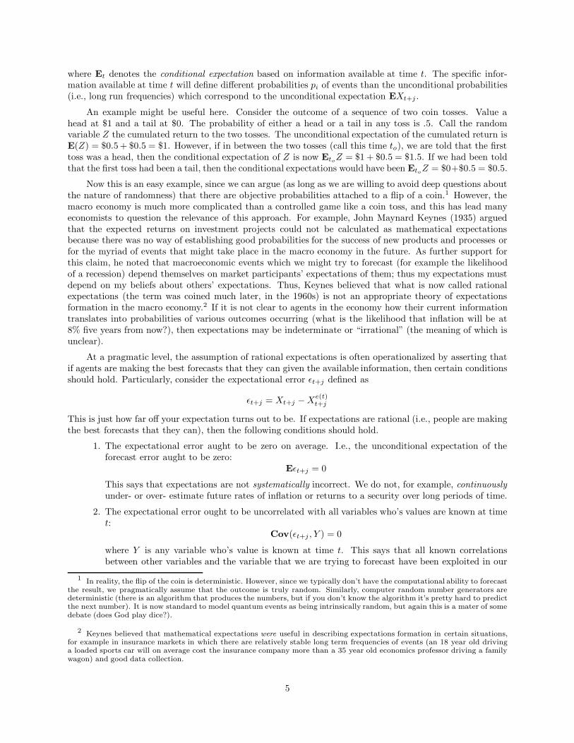
where Et denotes the conditional expectation based on information available at time t. The specific infor-mation available at time t will define different probabilities pi of events than the unconditional probabilities(i.e., long run frequencies) which correspond to the unconditional expectation EXt+j .

An example might be useful here. Consider the outcome of a sequence of two coin tosses. Value ahead at $1 and a tail at $0. The probability of either a head or a tail in any toss is .5. Call the randomvariable Z the cumulated return to the two tosses. The unconditional expectation of the cumulated return isE(Z) = $0.5 + $0.5 = $1. However, if in between the two tosses (call this time to), we are told that the firsttoss was a head, then the conditional expectation of Z is now Eto

Z = $1 + $0.5 = $1.5. If we had been toldthat the first toss had been a tail, then the conditional expectations would have been Eto

Z = $0+$0.5 = $0.5.

Now this is an easy example, since we can argue (as long as we are willing to avoid deep questions aboutthe nature of randomness) that there are objective probabilities attached to a flip of a coin.1 However, themacro economy is much more complicated than a controlled game like a coin toss, and this has lead manyeconomists to question the relevance of this approach. For example, John Maynard Keynes (1935) arguedthat the expected returns on investment projects could not be calculated as mathematical expectationsbecause there was no way of establishing good probabilities for the success of new products and processes orfor the myriad of events that might take place in the macro economy in the future. As further support forthis claim, he noted that macroeconomic events which we might try to forecast (for example the likelihoodof a recession) depend themselves on market participants’ expectations of them; thus my expectations mustdepend on my beliefs about others’ expectations. Thus, Keynes believed that what is now called rationalexpectations (the term was coined much later, in the 1960s) is not an appropriate theory of expectationsformation in the macro economy.2 If it is not clear to agents in the economy how their current informationtranslates into probabilities of various outcomes occurring (what is the likelihood that inflation will be at8% five years from now?), then expectations may be indeterminate or “irrational” (the meaning of which isunclear).

At a pragmatic level, the assumption of rational expectations is often operationalized by asserting thatif agents are making the best forecasts that they can given the available information, then certain conditionsshould hold. Particularly, consider the expectational error εt+j defined as

εt+j = Xt+j − Xe(t)t+j

This is just how far off your expectation turns out to be. If expectations are rational (i.e., people are makingthe best forecasts that they can), then the following conditions should hold.

1. The expectational error aught to be zero on average. I.e., the unconditional expectation of theforecast error aught to be zero:

Eεt+j = 0

This says that expectations are not systematically incorrect. We do not, for example, continuously

under- or over- estimate future rates of inflation or returns to a security over long periods of time.

2. The expectational error ought to be uncorrelated with all variables who’s values are known at timet:

Cov(εt+j , Y ) = 0

where Y is any variable who’s value is known at time t. This says that all known correlationsbetween other variables and the variable that we are trying to forecast have been exploited in our

1 In reality, the flip of the coin is deterministic. However, since we typically don’t have the computational ability to forecastthe result, we pragmatically assume that the outcome is truly random. Similarly, computer random number generators aredeterministic (there is an algorithm that produces the numbers, but if you don’t know the algorithm it’s pretty hard to predictthe next number). It is now standard to model quantum events as being intrinsically random, but again this is a mater of somedebate (does God play dice?).

2 Keynes believed that mathematical expectations were useful in describing expectations formation in certain situations,for example in insurance markets in which there are relatively stable long term frequencies of events (an 18 year old drivinga loaded sports car will on average cost the insurance company more than a 35 year old economics professor driving a familywagon) and good data collection.

5

forecast. If this were not true, then we could improve our forecasts by taking these correlations intoconsideration. For example, if current raw materials prices are correlated with the general pricelevel three months in the future, then information on this “leading indicator” will be exploited in theformation of inflationary expectations. Similarly, if stock prices systematically behave differentlyin January than in other months, this typical behavior will be anticipated by market participants.

These conditions are very powerful and are the foundation of rational expectation econometrics.

To summarize, rational expectations is a formalization that can be used in building and solving economicmodels and can be used as an assumption to econometrically identify economic relationships involvingexpectations. Whether it is more valuable as an ideal benchmark for modeling or is a good empiricalapproximation to the real world is a matter of some debate. The Nobel prize in economics was sharedrecently by Eugene Fama and Robert Shiller who come out on opposite sides of that debate. Fama tendsto see the gyrations of prices in financial markets as reflecting efficient markets in which expectations areresponding rationally to new information about economic fundamentals, while Shiller sees the same gyrationsas reflecting excess volatility and bubbles driven by swings in irrational exuberance.

Below we consider a famous empirical test of Shiller’s for the presence of excess volatility in the data.

Are Stock Prices Excessively Volatile?

Rational expectations is one of the foundations of efficient market theory (EMT) in financial markettheory.

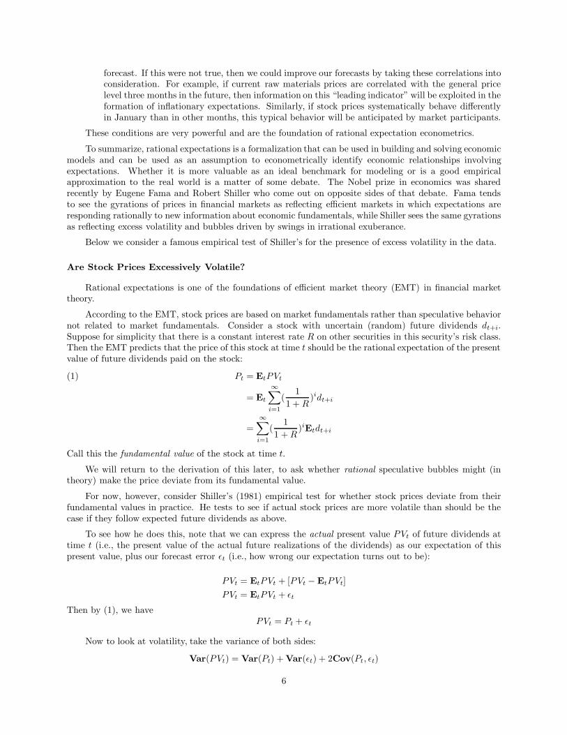
According to the EMT, stock prices are based on market fundamentals rather than speculative behaviornot related to market fundamentals. Consider a stock with uncertain (random) future dividends dt+i.Suppose for simplicity that there is a constant interest rate R on other securities in this security’s risk class.Then the EMT predicts that the price of this stock at time t should be the rational expectation of the presentvalue of future dividends paid on the stock:

Pt = EtPVt(1)

= Et

∞∑

i=1

(1

1 + R)idt+i

=

∞∑

i=1

(1

1 + R)iEtdt+i

Call this the fundamental value of the stock at time t.

We will return to the derivation of this later, to ask whether rational speculative bubbles might (intheory) make the price deviate from its fundamental value.

For now, however, consider Shiller’s (1981) empirical test for whether stock prices deviate from theirfundamental values in practice. He tests to see if actual stock prices are more volatile than should be thecase if they follow expected future dividends as above.

To see how he does this, note that we can express the actual present value PVt of future dividends attime t (i.e., the present value of the actual future realizations of the dividends) as our expectation of thispresent value, plus our forecast error εt (i.e., how wrong our expectation turns out to be):

PVt = EtPVt + [PVt − EtPVt]

PVt = EtPVt + εt

Then by (1), we havePVt = Pt + εt

Now to look at volatility, take the variance of both sides:

Var(PVt) = Var(Pt) + Var(εt) + 2Cov(Pt, εt)

6

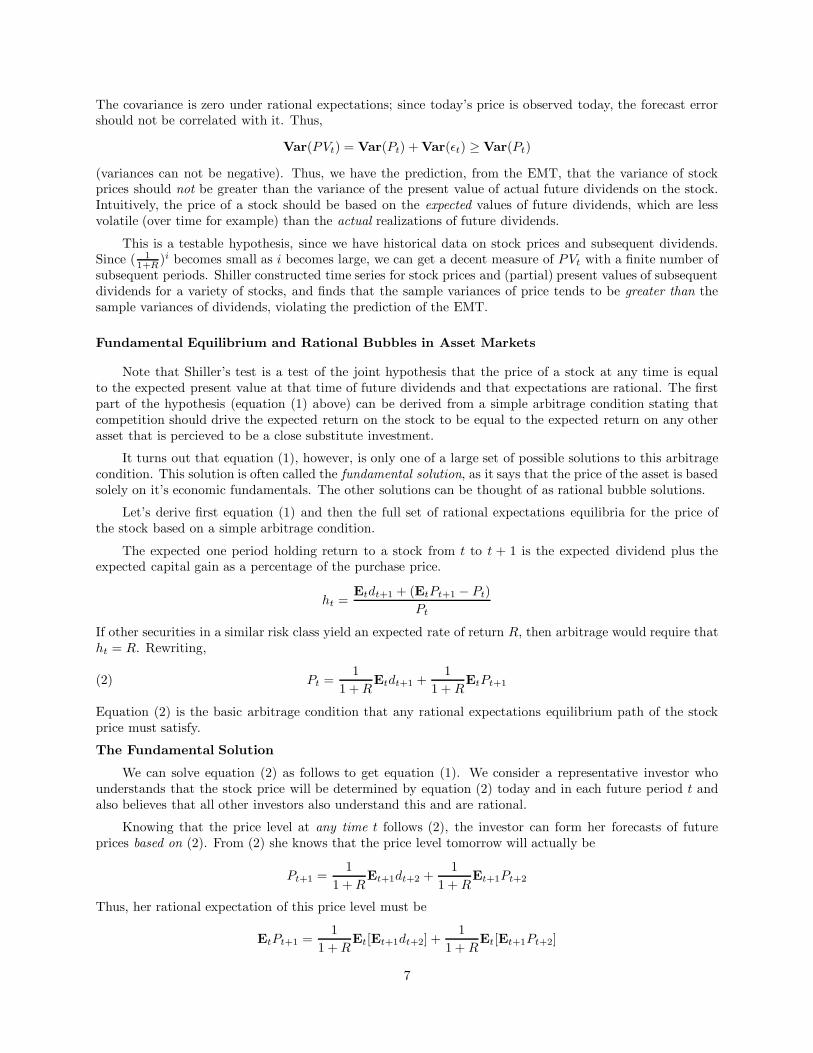
The covariance is zero under rational expectations; since today’s price is observed today, the forecast errorshould not be correlated with it. Thus,

Var(PVt) = Var(Pt) + Var(εt) ≥ Var(Pt)

(variances can not be negative). Thus, we have the prediction, from the EMT, that the variance of stockprices should not be greater than the variance of the present value of actual future dividends on the stock.Intuitively, the price of a stock should be based on the expected values of future dividends, which are lessvolatile (over time for example) than the actual realizations of future dividends.

This is a testable hypothesis, since we have historical data on stock prices and subsequent dividends.Since ( 1

1+R)i becomes small as i becomes large, we can get a decent measure of PVt with a finite number of

subsequent periods. Shiller constructed time series for stock prices and (partial) present values of subsequentdividends for a variety of stocks, and finds that the sample variances of price tends to be greater than thesample variances of dividends, violating the prediction of the EMT.

Fundamental Equilibrium and Rational Bubbles in Asset Markets

Note that Shiller’s test is a test of the joint hypothesis that the price of a stock at any time is equalto the expected present value at that time of future dividends and that expectations are rational. The firstpart of the hypothesis (equation (1) above) can be derived from a simple arbitrage condition stating thatcompetition should drive the expected return on the stock to be equal to the expected return on any otherasset that is percieved to be a close substitute investment.

It turns out that equation (1), however, is only one of a large set of possible solutions to this arbitragecondition. This solution is often called the fundamental solution, as it says that the price of the asset is basedsolely on it’s economic fundamentals. The other solutions can be thought of as rational bubble solutions.

Let’s derive first equation (1) and then the full set of rational expectations equilibria for the price ofthe stock based on a simple arbitrage condition.

The expected one period holding return to a stock from t to t + 1 is the expected dividend plus theexpected capital gain as a percentage of the purchase price.

ht =Etdt+1 + (EtPt+1 − Pt)

Pt

If other securities in a similar risk class yield an expected rate of return R, then arbitrage would require thatht = R. Rewriting,

(2) Pt =1

1 + REtdt+1 +

1

1 + REtPt+1

Equation (2) is the basic arbitrage condition that any rational expectations equilibrium path of the stockprice must satisfy.

The Fundamental Solution

We can solve equation (2) as follows to get equation (1). We consider a representative investor whounderstands that the stock price will be determined by equation (2) today and in each future period t andalso believes that all other investors also understand this and are rational.

Knowing that the price level at any time t follows (2), the investor can form her forecasts of futureprices based on (2). From (2) she knows that the price level tomorrow will actually be

Pt+1 =1

1 + REt+1dt+2 +

1

1 + REt+1Pt+2

Thus, her rational expectation of this price level must be

EtPt+1 =1

1 + REt[Et+1dt+2] +

1

1 + REt[Et+1Pt+2]

7

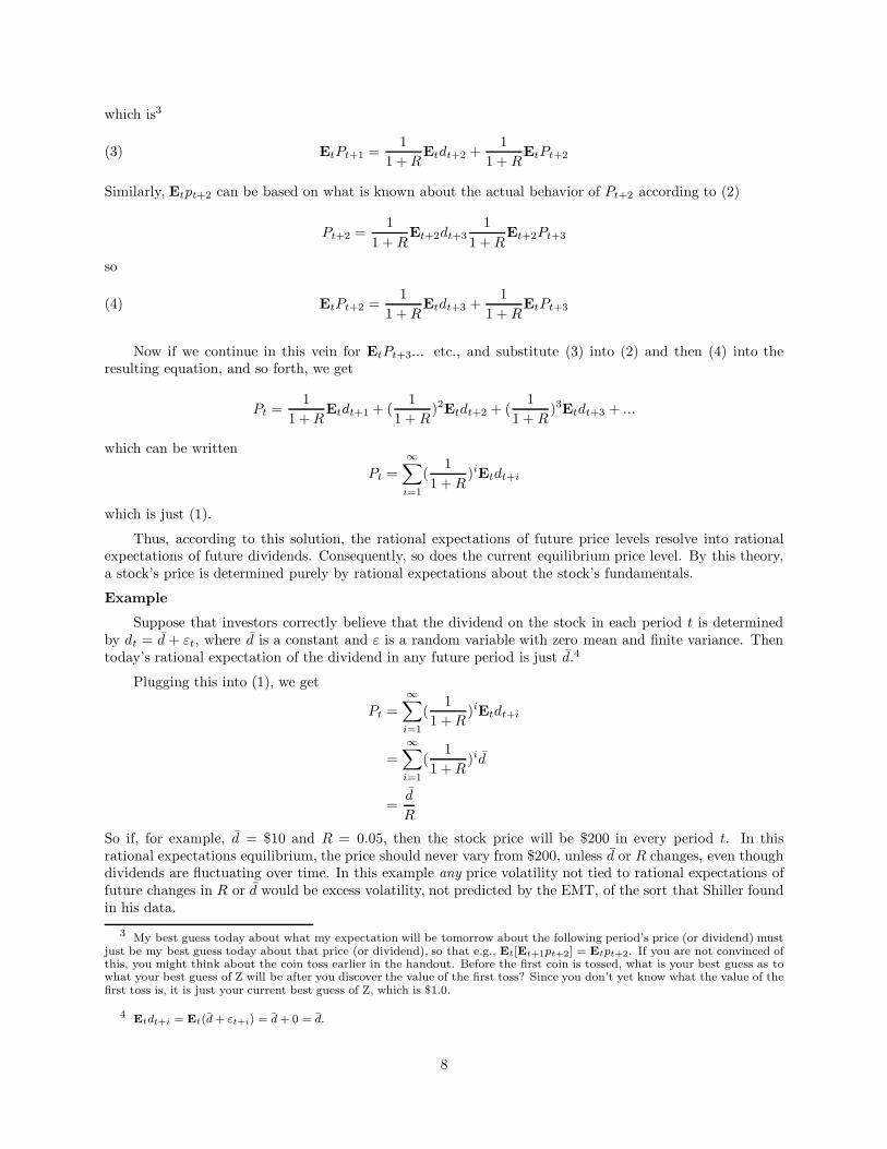
which is3

(3) EtPt+1 =1

1 + REtdt+2 +

1

1 + REtPt+2

Similarly, Etpt+2 can be based on what is known about the actual behavior of Pt+2 according to (2)

Pt+2 =1

1 + REt+2dt+3

1

1 + REt+2Pt+3

so

(4) EtPt+2 =1

1 + REtdt+3 +

1

1 + REtPt+3

Now if we continue in this vein for EtPt+3... etc., and substitute (3) into (2) and then (4) into theresulting equation, and so forth, we get

Pt =1

1 + REtdt+1 + (

1

1 + R)2Etdt+2 + (

1

1 + R)3Etdt+3 + ...

which can be written

Pt =

∞∑

i=1

(1

1 + R)iEtdt+i

which is just (1).

Thus, according to this solution, the rational expectations of future price levels resolve into rationalexpectations of future dividends. Consequently, so does the current equilibrium price level. By this theory,a stock’s price is determined purely by rational expectations about the stock’s fundamentals.

Example

Suppose that investors correctly believe that the dividend on the stock in each period t is determinedby dt = d̄ + εt, where d̄ is a constant and ε is a random variable with zero mean and finite variance. Thentoday’s rational expectation of the dividend in any future period is just d̄.4

Plugging this into (1), we get

Pt =

∞∑

i=1

(1

1 + R)iEtdt+i

=

∞∑

i=1

(1

1 + R)id̄

=d̄

R

So if, for example, d̄ = $10 and R = 0.05, then the stock price will be $200 in every period t. In thisrational expectations equilibrium, the price should never vary from $200, unless d̄ or R changes, even thoughdividends are fluctuating over time. In this example any price volatility not tied to rational expectations offuture changes in R or d̄ would be excess volatility, not predicted by the EMT, of the sort that Shiller foundin his data.

3 My best guess today about what my expectation will be tomorrow about the following period’s price (or dividend) mustjust be my best guess today about that price (or dividend), so that e.g., Et[Et+1pt+2] = Etpt+2. If you are not convinced ofthis, you might think about the coin toss earlier in the handout. Before the first coin is tossed, what is your best guess as towhat your best guess of Z will be after you discover the value of the first toss? Since you don’t yet know what the value of thefirst toss is, it is just your current best guess of Z, which is $1.0.

4Etdt+i = Et(d̄ + εt+i) = d̄ + 0 = d̄.

8

Bubble Solutions

However, (1) is only one solution to (2). To see this, let’s consider (2) under a very simple case.Specifically, simplify things by assuming perfect foresight and setting the actual and expected dividendstream constant over time. Then, rewriting (2) so that Pt+1 is on the left hand side, we have

(5) Pt+1 = −d̄ + (1 + R)Pt

The steady state equilibrium is P ∗ = d̄R

, the fundamental solution. Notice that you can solve for it here bysimply setting Pt = Pt+1.

However, since the coefficient on Pt is (1 + R) which is greater than one, the steady state solution is

unstable. If the price starts at d̄R

it will stay there forever. If it starts above this value, however, the pricelevel will follow a rational speculative bubble diverging from P ∗ over time at rate R. One way to see this isto simply plug a starting value for the price above the fundamental value into equation (12) above, and seethat the price will be even higher in the next period. If we iterate forward, the price will continue to growaway from the fundamental value over time at growth rate R.

The general solution to (5) is

(6) Pt = P ∗ + (1 + R)t(P0 − P ∗)

What is the intuition for these rational bubble solutions? Let’s continue with our example above inwhich d̄ = 10 and R = 0.05, so that P ∗ = 200. Then if you believe that the price will stay constant at$200, then the expected capital gain on the stock is zero, and the expected return is d̄/200 which is exactly0.05. So, in that case, you should be willing to pay up to $200 for the stock, as that is the price that leavesyou indifferent between the stock and other securities. This is indeed the fundamental value of the stock atwhich the EMT predicts that it will be priced.

Now, under what condition would you pay $300 for this stock? If you expected the price to rise by$5 during the period, then this expected capital gain of $5 plus the $10 dividend would yield the requiredexpected holding return of 5%. Therefore, Pt = $300 is a rational expectations equilibrium if EtPt+1 = $305.

And under what condition will the price actually be $305 in t + 1? For that to be the case, we needEtPt+2 = $310.25. I.e., if we expect the price to continue to grow away from $200 at 5% per year, every yearin the future, then this expectation will be self fulfilling, and the price level will follow exactly that path.

Similarly, suppose that you thought that the price may rise next period or the bubble might burst.Suppose for example that you believe that with probability 0.2 the price will fall back to $200 next period(the bubble will burst), and with probability 0.8 the price will rise next period (the bubble will continue).Then, it is rational to pay $300 for the stock today, if you believe that, if the bubble does not burst tomorrow,the price tomorrow will be $331.25. In that case, you believe that there is an 80% chance of getting a $31.25capital gain, and a 20% chance of a $100 capital loss, so that your expected capital gain is $5). Adding theexpected dividend of $10, your expected rate of return on the stock is exactly 5%.

So ‘rational’ bubbles are theoretically possible. Whether they are plausible or empirically relevant is amatter of some controversy.

Among possible objections to these bubble solutions are the following. First, how will a large numberof independent economic actors coordinate on a particular initial value of the price level other than P = P ∗.Of course the same criticism can be levied at the fundamental solution P = P ∗. Second, why should anyoneexpect that the price of the stock can rise indefinitely in the absence of rising dividends? Once a bubblestarts, above, it must continue on forever. If the public does not believe that the price can grow forever,then the only solution to (2) left is the fundamental solution.

However, an alternative to believing that a bubble will last forever is to expect any bubble to bursteventually, but not to know with certainty when it will end. The public might, for example, collectivelycoordinate the timing of bubbles with the outcomes of otherwise irrelevant events. Such equilibria are called

9

sunspot equilibria. Again, skeptics would argue that these rational bubbles are unreasonable in that theyrequire the public to believe that the bubble could continue for a long time (and to act on this belief).

Some skeptics of rational bubbles therefore prefer the fundamental rational expectations solution, whileothers argue that bubbles are indeed relevant, but that they are not grounded in rational behavior, ratherin irrational or boundedly rational behavior. For example, some investors may buy into a bubble becausethey are blindly following the trend, or may believe that the bubble will burst but are optimistic that theywill be among the ones to get out first leaving others to hold the bag. As noted before, Shiller falls into thecategory of economists who believe both that there is widespread excess volatility and that this volatility isdriven by less than fully rational behavior.

Bounded Rationality and Learning

While rational expectations is a very strong modeling assumption, it is considered to be an importantmodeling benchmark (how does the model behave if agents in it have rational expectations).

There may also be a back-door rationale for using rational expectations in macroeconomic modeling.Suppose that in reality, many economic agents have fairly naieve expectations, but learn over time from theirmistakes. Then this learning may cause expectations to converge to rational expectations over time.

To see this, let’s consider condition (2) again, but drop the assumption of rational expectations. Let’salso simplify by assuming that the dividend stream is constant at d̄, and that the investor knows this. Inthis case, (2) is:

(2’) Pt =1

1 + Rd̄ +

1

1 + RP

e(t)t+1

Now let’s assume that the investor has a naive expectation that that the price level in the future will beconstant at some level P̃ . Then, by (2′), the actual price level today will be

(7) Pt =1

1 + Rd̄ +

1

1 + RP̃

which can be written in terms of P ∗ as follows

(8) Pt = P ∗ + (P̃ − P ∗

1 + R)

We can see by (8) that Pt lies between P ∗ and P̃ . So given the expectation that the price in the next

period will be P̃ , arbitrage between the stock and the bond makes the actual equilibrium price lie betweenthis expectation and the fundamental rational expectations equilibrium P ∗. If investors stick to their fixedexpectations, then they will see over time that this expectation is systematically wrong every period. If theyeventually learn to recognize their mistake, they will adjust their expectation toward the actual price, whichis also in the direction of the rational expectations equilibrium price P ∗. Thus, over time, learning will driveboth the expected price P̃ and the actual equilibrium price P toward P ∗.

For example, if d̄ = $10 and R = 0.05, so that P ∗ = 200, suppose that the average investor believedthat the price tomorrow would be $250. Then by arbitrage (2′) the price today will be Pt = 260

1.05 = $247.62.Now suppose that after seeing that the price today was $247.62, investors update their expectations in thefollowing period so that P̃t+1 = $247.62. Then the actual price in period t+1 will be Pt+1 = 257.62

1.05= $245.35.

So as expectations adapt to the actual history of prices, both expected and actual price gravitates in thedirection of P ∗ = 200. Once P̃ reaches 200, then P and P̃ will both stay at $200.

So we see that in this very simple case, learning should eventually drive expectations to be rational.Indeed, in this example, learning selects the fundamental rational expectations equilibrium (not rationalbubble solutions to the model). So at least in this very simple example, learning supports the EMT as alonger run outcome, rather than as a condition that is fulfilled in every period.

10

Before we get too excited about this result however, note that for adaptive expectations to respondrationally in a changing environment, the learning process would have to be substantially more sophisticated.Some economists have argued that we should expect this to be the case, while others (including myself)remain skeptical. See Georges (2008) for a discussion of how learning can fial to converge to rationalexpectations.

References

Georges, Christophre, “Bounded Memory, Overparameterized Forecast Rules, and Instability,” Eco-

nomics Letters, 98, 2008, 129–135.

Keynes, John Maynard, The General Theory of Employment, Interest, and Money, 1935.

Shiller, Robert, “Do Stock Prices Move Too Much to be Justified by Subsequent Changes in Dividends?,”American Economic Review, 71, 1981, 421–436.

11

Appendix (optional)

Digression on Solutions to Difference Equations

Consider a first order linear difference equation in a variable x with constant coefficients a and b:

(9) xt+1 = a + b xt

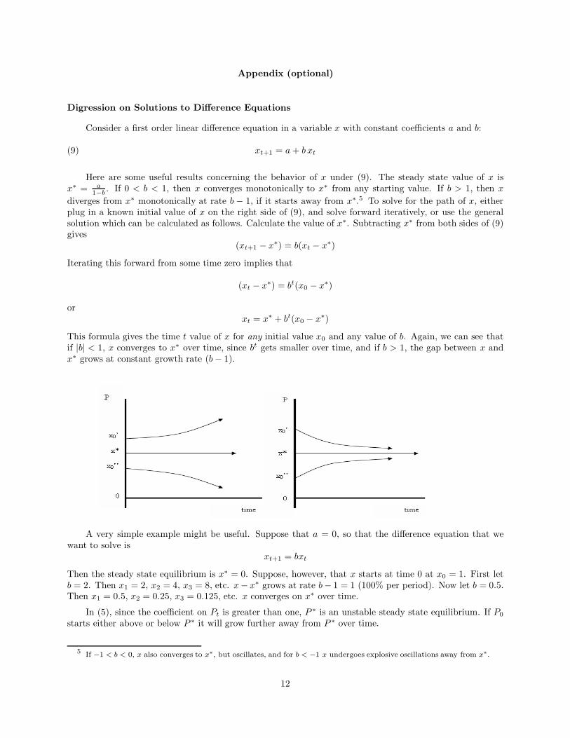
Here are some useful results concerning the behavior of x under (9). The steady state value of x isx∗ = a

1−b. If 0 < b < 1, then x converges monotonically to x∗ from any starting value. If b > 1, then x

diverges from x∗ monotonically at rate b − 1, if it starts away from x∗.5 To solve for the path of x, eitherplug in a known initial value of x on the right side of (9), and solve forward iteratively, or use the generalsolution which can be calculated as follows. Calculate the value of x∗. Subtracting x∗ from both sides of (9)gives

(xt+1 − x∗) = b(xt − x∗)

Iterating this forward from some time zero implies that

(xt − x∗) = bt(x0 − x∗)

orxt = x∗ + bt(x0 − x∗)

This formula gives the time t value of x for any initial value x0 and any value of b. Again, we can see thatif |b| < 1, x converges to x∗ over time, since bt gets smaller over time, and if b > 1, the gap between x andx∗ grows at constant growth rate (b − 1).

A very simple example might be useful. Suppose that a = 0, so that the difference equation that wewant to solve is

xt+1 = bxt

Then the steady state equilibrium is x∗ = 0. Suppose, however, that x starts at time 0 at x0 = 1. First letb = 2. Then x1 = 2, x2 = 4, x3 = 8, etc. x− x∗ grows at rate b− 1 = 1 (100% per period). Now let b = 0.5.Then x1 = 0.5, x2 = 0.25, x3 = 0.125, etc. x converges on x∗ over time.

In (5), since the coefficient on Pt is greater than one, P ∗ is an unstable steady state equilibrium. If P0

starts either above or below P ∗ it will grow further away from P ∗ over time.

5 If −1 < b < 0, x also converges to x∗, but oscillates, and for b < −1 x undergoes explosive oscillations away from x∗.

12