Rate Types for Stream Programs

Thomas W. Bartenstein and Yu David LiuSUNY Binghamton

Binghamton, NY13902, USA{tbarten1, davidL}@binghamton.edu

AbstractWe introduce RATE TYPES, a novel type system to reasonabout and optimize data-intensive programs. Built aroundstream languages, RATE TYPES performs static quantita-tive reasoning about stream rates — the frequency of dataitems in a stream being consumed, processed, and produced.Despite the fact that streams are fundamentally dynamic,we find two essential concepts of stream rate control —throughput ratio and natural rate — are intimately relatedto the program structure itself and can be effectively rea-soned about by a type system. RATE TYPES is proven tocorrespond with a time-aware and parallelism-aware oper-ational semantics. The strong correspondence result toler-ates arbitrary schedules, and does not require any synchro-nization between stream filters. We further implement RATETYPES, demonstrating its effectiveness in predicting streamdata rates in real-world stream programs.

Categories and Subject Descriptors D.3.2 [ProgrammingLanguages]: Language Classifications — Data-flow lan-guages; D.4.8 [Programming Languages]: Performance —Modeling and Prediction; F.3.3 [Theory of Computation]:Studies of Program Constructs — Type structure

Keywords Stream programming; data processing rates;data throughput; performance reasoning; type systems

1. IntroductionBig Data and parallelism are two dominant themes in mod-ern computing, both of which call for language supportoffered naturally by the stream programming model. Astream program consists of data-processing units (called fil-ters) connected by paths to indicate the data flow. At runtime, each such path is occupied by an ordered, potentially

Permission to make digital or hard copies of all or part of this work for personal orclassroom use is granted without fee provided that copies are not made or distributedfor profit or commercial advantage and that copies bear this notice and the full citationon the first page. Copyrights for components of this work owned by others than ACMmust be honored. Abstracting with credit is permitted. To copy otherwise, or republish,to post on servers or to redistribute to lists, requires prior specific permission and/or afee. Request permissions from permissions@acm.org.OOPSLA ’14, October 20–24, 2014, Portland, Oregon, USA.Copyright © 2014 ACM 978-1-4503-2585-1/14/10. . . $15.00.http://dx.doi.org/10.1145/2660193.2660225

Figure 1. Throughput Ratio and Natural Rate

large sequence of data items, called data streams. Streamprogramming — together with its close relatives of signalprogramming and (more generally) dataflow programming— are successful in scientific computing [1], graphics [2],databases [3], GUI design [4, 5], robotics [6], sensor net-works [7], and network switches [8]. Its growing popularityalso generates significant interest in developing theoreticalfoundations for stream programming [9–11].

In this paper, we develop a novel theoretical founda-tion and practical implementation to reason about the datarate aspect of stream programming. The centerpiece of thiswork is RATE TYPES, a type system to reason about streamrates, i.e., how frequently data can be consumed, processed,and produced. Despite the fundamentally dynamic nature ofstreams, we show that two crucial characteristics of streamapplications can be reasoned about:

Throughput Ratio: the relative ratio between the outputstream rate and the input stream rate of a stream program.

Natural Rate: the output stream rate of a stream programgiven an unlimited input stream rate.

We use Figure 1 to illustrate these concepts. Intuitively,as the the rate of data flowing into the stream program (theinput stream rate) increases, the rate of data flowing out thesame program (the output stream rate) should increase. Theproportionality of increase is represented by the throughputratio, with a bound illustrated by the slope of the slanteddotted (green) line in Figure 1. However, the output streamrate cannot grow infinitely even if the input stream rate

keeps increasing, because it takes time to process data, i.e.,taking data from the input stream, performing calculationson that data, and putting the results on the output stream.Eventually, the output stream will reach a “plateau” — thebound of the natural rate — as illustrated by the horizontaldotted (red) line in Figure 1. This phenomenon is supportedby our experiments. The solid (blue) curve in the sameFigure illustrates the experimentally measured output streamrates during a real program execution, as measured for manydifferent input stream rates.

Our key insight is that both throughput ratio and natu-ral rate are closely related to the program structure, whichin turn can be effectively reasoned about by type systems.RATE TYPES models both concepts as types, and provides aunified type checking and inference framework to help an-swer a wide range of performance-related questions, suchas whether a video “decoder” stream program can produce3241 data items (e.g., pixels) a second when being fed with1208 raw data items per second. Make no mistake: it wouldbe unreasonable to expect such performance-focused ques-tions to be answered completely without any knowledgeof the run-time. What is less obvious — and what RATETYPES illuminates — is how little such knowledge is re-quired to enable full-fledged reasoning, so that crucial per-formance questions such as data throughput can largely beanswered analytically rather than experimentally. Along thisline, RATE TYPES is an instance of quantitative reasoningabout performance-related properties, an active area of re-search (e.g., [12–15]), with a focus on data-flow program-ming models. To the best of our knowledge, RATE TYPESis the first result for stream rate reasoning, in a general con-text that requires neither static scheduling [16] nor inter-filtersynchronization [17].

RATE TYPES promotes a type-theoretic approach to rea-son about data rates, bringing benefits long known to typesystem research to the emerging application domain of data-intensive software: (1) type systems excel at relating andpropagating information characteristic of program struc-tures, throughput ratio and natural rate in our system; (2)type systems have strong support for modularity, which inour case spearheads a flavor of compositional performancereasoning; (3) type systems have “standard” and provablycorrect ways to construct and connect a series of algorithms— such as establishing the connection between type check-ing and type inference, and determining principal types —which in RATE TYPES happen to unify many interestingpractical algorithms in stream rate control.

To bring RATE TYPES closer to real-world computing,we implement our type inference system on top of theStreamIt language [18], predicting data throughput underdifferent settings of data input/output stream rates. Our ex-perimental results demonstrate close resemblance betweenthe reasoning results and the measured results.

This paper makes the following contributions:

• It develops a type system to reason about throughputratio and natural rate of stream programs, and formallyestablishes the correlation between the stream rates fromthe reasoning system and those manifest at run time – asa strong correspondence property between the static andthe dynamic.

• It defines a type inference to infer the throughput ratioand the natural rate. The inference is sound and completerelative to type checking, and further enjoys principaltyping — the existence of upper bound for throughputratio and natural rate.

• It describes a prototyped implementation of the type sys-tem, with experimental results demonstrating the effec-tiveness of the formal reasoning in predicting runtimestream program behaviors.

2. Stream Programming and ReasoningWe now outline the basics of stream programming, and in-formally describe how RATE TYPES can help reason aboutstream programs. Our type system can be built around a va-riety of programming languages. Here we choose StreamIt[18] as the host language, and discuss other applicable lan-guages at the end of the section as well as in later sections ofthe paper.

Stream Programming Figure 2 outlines an example streamprogram for simulated annealing [19], a classic optimizationalgorithm that probabilistically finds globally optimal solu-tions using a randomized locally optimal search. Given seedcoordinates as the input stream, this program fragment (en-try at anneal in Line 3) takes each input coordinate, checksits 8 neighbors in the 2D space, and picks the coordinate inthe neighborhood with best benefit (checkNeighbors inLine 10). This coordinate is fed back for the next round ofspace search. The neighborhood-based strategy may trap thesearch to a local, but not global, optimality. Thus, the pro-gram has with a “jump” strategy to allow some coordinatesto be randomly mutated (randomJump in Line 45).

The base processing unit of a stream program is a filter,like getNeighbors in Line 15, whose body is a functionlabeled with keyword work. A filter execution instance,informally called a filter firing, takes in a pre-defined finitenumber of data items from the input stream (through pop)and places a finite number of data items to the output stream(through push). For instance in Lines 17-21, the filter places9 coordinates on the output stream for each coordinate itreads from the input stream. A filter can only be launchedwhen there are enough data items on the input stream, asspecified by the pop declaration in the filter signature (thedeclarations immediately after the keyword work).

A filter such as getNeighbors can execute in parallelwith a different filter, such as evalNeighbors, as longas each filter has sufficient data items in their respectiveinput streams, Similar to other concurrency models such as

1 s t r u c t xy { i n t x ; i n t y ; i n t ben ; }2

3 xy�xy f eedbackloop a n n e a l ( ) {4 j o i n roundrobin ( 1 , 9 9 ) ;5 body c h e c k N e i g h b o r s ;6 loop randomJump ;7 s p l i t roundrobin ( 1 , 9 9 ) ;8 }9

10 xy�xy p i p e l i n e c h e c k N e i g h b o r s ( ) {11 add g e t N e i g h b o r s ;12 add c o m p u t e P r o f i t s ;13 add e v a l N e i g h b o r s ;14 }

15 xy�xy f i l t e r g e t N e i g h b o r s ( ) {16 work push 9 pop 1 {17 xy p = pop ( ) ;18 push ( p ) ;19 push ({p . x +1 , p . y , p . ben } ) ;20 push ({p . x , p . y +1 , p . ben } ) ;21 . . .22 }}23 xy�xy s p l i t j o i n c o m p u t e P r o f i t s ( ) {24 s p l i t roundrobin ( 1 , 1 ) ;25 add g e t P r o f i t ;26 add g e t P r o f i t ;27 j o i n roundrobin ( 1 , 1 ) ;28 }29 xy�xy f i l t e r g e t P r o f i t ( ) {30 work push 1 pop 1 {31 xy l o c =pop ( ) ;32 l o c . ben= . . . ; / / f i n d p r o f i t33 push ( xy ) ;34 }}

35 xy�xy f i l t e r e v a l N e i g h b o r s ( ) {36 work push 1 pop 9 {37 xy p1 = pop ( ) ,38 p2=pop ( ) ,39 . . .40 p9 = pop ( ) ;41 xy b e s t = . . . ; / / b e s t o f 942 push ( b e s t ) ;43 }}44

45 xy�xy f i l t e r randomJump ( ) {46 work push 1 pop 1 {47 xy p = pop ( ) ;48 xy rand = . . . ;49 i f ( . . . ) push ( p )50 e l s e push ( r and ) ;51 }}

Figure 2. A StreamIt Program for Simulated Annealing

actors [20], a filter execution instance abides by a “one firingat a time” rule: the evaluation of each filter function bodyupon application must be completed before the second filterexecution instance can start.

To stay neutral to the terminology of host languages,we name the 3 most commonly used filter combinators asfollows:

• Chain (pipeline in StreamIt): connects the outputstream of one sub-program to the input stream of another.For example, checkNeighbors in Line 10 “chains”the output stream of getNeighbors with the inputstream of computeProfits.

• Diamond (splitjoin in StreamIt): dissembles and as-sembles data streams. For example, computeProfitsin Line 23 says that the data items on the input streamwill be alternatively placed to the input streams of thetwo getProfit execution instances, whose respectiveoutput streams will be alternatively selected to assemblethe output stream of computeProfits. Declarationroundrobin (1,1) indicates a 1:1 alternation.

• Circle (feedbackloop in StreamIt): a combinatorto support data feedback. For example, anneal inLine 3 says that for every 100 coordinates producedby checkNeighbors, 99 are fed back for random-Jump processing. Every time 99 coordinates are pro-duced by randomJump, 1 more new coordinate (addi-tional “seed” coordinates) will be admitted for annealing.

Stream Reasoning For stream applications such as simu-lated annealing, high performance is often a matter of ne-cessity due to copious data volume. High on the wish list ofa data engineer is the ability to reason about performance,with questions such as:

Q1: Is it possible for a program to sustain the production ofn2 data items per second when its input is fed with n1

items per second?

Q2: Is it possible for a program to sustain the productionof n data items per second given unlimited rates for datainputs?

Q3: If a program is targeted at producing n data items persecond, what is the minimal rate of feeding data at itsinput?

Q4: Given the program is fed with n data items per second,what is the expected rate for its data production?

RATE TYPES addresses Q1-2 through type checking, andQ3-4 through type inference. It further demonstrates therelationship among these questions in a unified, provablycorrect framework.

For example, through answering Q4, RATE TYPES iscapable of demonstrating that the output rate is limited bothby the rate at which data items are supplied to the program,and by the inherent limits of the program sub-components.Overall, it provides a rigorous explanation to the shape ofthe curve we introduced in Figure 1. Consider a simple filtersuch as getProfit at line 29 in Figure 2 and assumeit takes three seconds from the pop to the push. If dataarrives at the input stream every five seconds, say at times3, 8, 13, . . . , then the filter will process that data and writeto the output stream once every five seconds as well, forinstance at times 6, 11, 16, . . . . Even though these timesare offset from the input, the rate at which they appear isstill directly proportional to the input rate. If, however, dataarrive at getProfit every two seconds, say at times 5,7, 9, . . . , then the performance of the getProfit filterdominates the output rate, and pushes to the output streamwill occur at times 8, 10, 12, . . . , once every three seconds.RATE TYPES generalizes this simple concept to reason aboutthe stream rates throughout the program, and shows that anentire program can be characterized by the proportion of theinput rate to the output rate, or the throughput ratio, as wellas an internal stream program “speed limit” - the maximumpossible output rate, independent from the input stream rate,which we call the natural rate of the program.

The formal sections of this paper define a stream-orientedlanguage core, and formally define

• an operational semantics (Section 3) where the notion ofstream rates can be established;

• a type checking system (Section 4.1) where throughputratio and natural rate can be reasoned about, e.g., an-swering questions such as if one filter has throughputratio of 1

3 and the other has throughput ratio of 14 , then

the program with the two filters chained together shouldhave throughput ratio of 1

12 . The type checking system isimportant for compositional reasoning, in that through-put ratio and natural rate of a program can still be rea-soned about, even though the implementation of sub-stream graphs of the program may not be known (as longas their types are known).

• a type inference algorithm (Section 4.2) where the de-pendencies between the rates of individual streams ina stream program runtime are abstracted as linear con-straints. The type inference algorithm is important for an-swering questions such as what the maximum throughputratio and natural rate are for a program.

The paper further establishes several important propertiesof RATE TYPES. To highlight a few:

• Static/Dynamic Correspondence (Theorem 1): we showthat RATE TYPES correctly captures the dynamic behav-ior as defined by the operational semantics: specifically,both the throughput ratio and natural rate we reason aboutstatically are a faithful approximation of dynamic streamrates.

• Soundness and Completeness of Inference (Theorem 3and Theorem 4): we show that the inference algorithmcorrectly infers the throughput ratio and natural rate of aprogram, and can infer any throughput ratio and naturalrate for which the type checking algorithm can establisha type derivation.

• Principal Typing of Inference (Theorem 5): the maximumthroughput ratio and natural rate exist.

Assumption Every reasoning framework needs to addressthe base case of reasoning: to type an arithmetic expression,the assumption is that integers are of int type; to verifya program is secure, one needs to know password stringsare properly associated with high security labels. In RATETYPES, the base case is the filter, and the assumption wemake is its execution time can be predetermined and speci-fied.

At a first glance, this assumption may seem counter-intuitive to what is conventionally considered as “static.” Wehowever believe this is reasonable because (a) filter behav-iors are much more predictable than full-fledged programs,thanks to the non-shared memory model they routinely adoptand their lack of side effects often called for in real-world

stream languages [18, 21, 22]; (b) formal systems to rea-son about individual filter behaviors exist [10]; (c) Experi-mentally, filter execution time is known to be stable throughprofiling; Core optimizations of the StreamIt compiler [23]rely on it; (d) real-world software development is iterative.Profiling-guided typing is not new [24]. What ultimatelymatters is to help programmers reason about performanceat some point during the software life cycle.

Applicability RATE TYPES is primarily designed for ex-pressive and general-purpose stream languages. The frame-work may be applied more broadly to systems where dataprocessing is periodic, and/or where rates matter: (a) sensornetwork languages (e.g., [7]), where determining the low-est sensing rate possible is relevant; (b) signal languagessuch as FRP [6]. Even though the input signals are theoret-ically continuous in this context, practical implementationsare still concerned with sampling rate. In addition, even ifall input signals are continuous — a case analogous to Q2— the output signal is still discrete where rates may matter.(c) high-performance-oriented dataflow composition frame-works such as FlumeJava [25] and ParaTimer [26], wheresingle MapReduce-like units are composed together in ex-pressive ways. In Section 6, we will have a more in-depthdiscussion on how RATE TYPES can be mapped to a varietyof existing frameworks.

3. Syntax and Dynamic SemanticsAbstract Syntax The abstract syntax of our language isdefined as follows:

P ::= FL[ni, no] | P �` P ′ | programP3δ,αP ′ | P �`

′,`α,δ P

′

δ ::= 〈n;n′〉 distribution factorα ::= 〈n;n′〉 aggregation factor

The building block of a stream program, a filter, takes thesyntactic form of FL[ni, no], where F is the filter functionbody, and L is a unique program label called a filter label.Filter labels range over the set of FLAB. Each filter is furtherdeclared with two natural numbers: ni for the number ofitems to be consumed by an invocation of the filter, and nofor the number of items to be produced by an invocation. Thetwo numbers correspond to the pop and push declarationsin Figure 2. Let NAT represent natural numbers startingfrom 1. Metavariable n ranges over NAT. For each filter, wefurther require F to be an element of DATAni → DATA

no

where DATA is the set of data items.The remaining syntactic forms of a program P corre-

spond to the three combinators in stream programming: achain composition, a diamond composition, and a circlecomposition; represented in the grammar in that order. If aprogram P takes the form of one of these combinators, weinformally say that PA and PB are sub-programs of P . Forthe circle composition, PA �

`′,`α,δ PB , we further informally

call PA the forward sub-program and PB the feedback sub-program.

For both diamond and circle compositions, metavariablesδ = 〈n;n′〉 and α = 〈n;n′〉 represent the distribution factorand the aggregation factor respectively. They correspond tothe tuples succeeding the split keyword and the joinkeyword in the Figure 2 example respectively. Intuitively,the distribution factor specifies the proportion of splitting adata stream into two, and the aggregation factor specifies thatof joining two data streams into one.

For the purpose of formal development, each chain ex-pression is associated with a distinct stream label, `, andeach circle expression is associated with two stream la-bels. The motivation of representing them in the syntaxwill be made clear later. Metavariable ` ranges over setSLAB. Given a program P , we use flabels (P ) to enu-merate all filter labels in P , and slabels (P ) to enumerateall stream labels in P . The flabels definition is obvious,and slabels is inductively defined as follows:

slabels“FL[ni, no]

”, ∅

slabels“PA �

` PB”, slabels (PA)∪

slabels (PB) ∪ {`}slabels (PA3δ,αPB) , slabels (PA) ∪ slabels (PB)

slabels“PA �

`′,`α,δ PB

”, slabels (PA)∪

slabels (PB) ∪ {`, `′}

In Appendix A, we show the simple syntax core is capa-ble of encoding other programming patterns, such as k-waysplit-join and non-round-robin distribution/aggregation.

The program in Figure 2 can be represented by our syntaxas Panneal where:

Panneal =PcheckNeighbors �`0,`1〈1;99〉,〈1;99〉 PrandomJump

PcheckNeighbors =(PgetNeighbors �`2 PcomputeProfits)

�`3 PevalNeighbors

PgetNeighbors =FL1 [1, 9]

PcomputeProfits =FL2 [1, 1]3〈1;1〉;〈1;1〉FL3 [1, 1]

PevalNeighbors =FL4 [9, 1]

PrandomJump =FL5 [1, 1]

In the rest of the paper, we use notation [X1, . . . , Xn] torepresent a sequence with elements X1, . . . , Xn, or sim-ply X when sequence length does not matter. Furthermore,we define |[X1, . . . , Xn]| def= n and use comma for se-quence concatenation, i.e. [X1, . . . , Xn], [Y1, . . . , Yn′ ]

def=[X1, . . . , Xn, Y1, . . . Yn′ ]. We call a sequence in the formof [X1 7→ Y1, . . . Xn 7→ Yn] a mapping sequence if X1,

|S| < (n+ n′)

S '〈n;n′〉 ∅; ∅

S2 = SA2, SB2

|SA2| = n |SB2| = n′

S1 '〈n,n′〉 SA1, SB1

S1, S2 '〈n;n′〉 SA1, SA2;SB1, SB2

(|SA| < n) ∨ (|SB | < n′)

SA;SB .〈n;n′〉 ∅

|SA2| = n |SB2| = n′

S2 = SA2, SB2

SA1, SB1 .〈n;n′〉 S1

SA1, SA2;SB1, SB2 .〈n;n′〉 S1, S2

Figure 3. Distribution and Aggregation

. . . , Xn are distinct. We equate two mapping sequences ifone is a permutation of elements of the other. Let map-ping sequence M = [X1 7→ Y1, . . . Xn 7→ Yn]. We fur-ther define dom (M) def= {X1, . . . , Xn} and ran (M) def={Y1, . . . , Yn} and use notation M(Xi) to refer Yi for any1 ≤ i ≤ n. Binary operator ] is defined as M1 ] M2 =M1,M2 iff dom (M1) ∩ dom (M2) = ∅. The operator is oth-erwise undefined.

Stream Runtime The following structures are used fordefining the stream runtime:

R ::= ` 7→ S program runtimeS ::= d stream` ∈ SLAB ∪ {`IN, `OUT} stream labelt ∈ TIME ⊆ REAL+ timed ∈ DATA data itemΠ ∈ FLAB 7→ TIME filter time mapping

The runtime,R, consists of a mapping sequence from streamlabels to streams. A stream is defined as a list of data items.Two built-in stream labels, `IN and `OUT are used to facilitatethe semantics development. Given a program P , `IN and `OUTlabels the input stream and the output stream of P . Mappingfunction Π maps each filter (label) to its execution time.

Ternary predicate S 'δ SA, SB holds when S canbe “split” to SA and SB using distribution factor δ, andSA, SB .α S holds when SA and SB can be “joined” to-gether as S with aggregation factor α. Their formal defini-tions are in Figure 3. Some examples should demonstratethe functionality of these predicates.

[1, 2, 3, 4, 5, 6] '〈1;2〉 [1, 4], [2, 3, 5, 6][1, 4], [2, 3, 5, 6] .〈1;2〉 [1, 2, 3, 4, 5, 6]

[1, 2, 3, 4, 5, 6, 7] '〈1;2〉 [1, 4], [2, 3, 5, 6][1, 4, 7], [2, 3, 5, 6] .〈1;2〉 [1, 2, 3, 4, 5, 6]

RP−→tR

[D-Reflex]R

P−→t1

R′ R′P−→t2

R′′ t1 + t2 ≤ t

RP−→tR′′

[D-Trans]

So2 = F (Si1) |Si1| = ni |So2| = no Π(L) ≤ t

[`IN 7→ (Si2, Si1), `OUT 7→ So1]FL[ni,no]−−−−−−→

t[`IN 7→ Si2, `OUT 7→ (So2, So1)]

[D-Filter]

R = RA ]RB ] [`IN 7→ Si, `OUT 7→ So, ` 7→ S]R′ = R′A ]R′B ] [`IN 7→ S′i, `OUT 7→ S′o, ` 7→ S′]S = S2, S1 S′ = S3, S2

RA ] [`IN 7→ Si, `OUT 7→ S2]PA−−→tA

R′A ] [`IN 7→ S′i, `OUT 7→ S′] tA ≤ t

RB ] [`IN 7→ S, `OUT 7→ So]PB−−→tB

R′B ] [`IN 7→ S2, `OUT 7→ S′o] tB ≤ t

RPA�

`PB−−−−−−→t

R′[D-Chain]

R = RA ]RB ] [`IN 7→ Si, `OUT 7→ So]R′ = R′A ]R′B ] [`IN 7→ S′i, `OUT 7→ S′o]

Si 'δ SA, SB S′i 'δ S′A, S′B SC , SD .α So S′C , S′D .α S′o

RA ] [`IN 7→ SA, `OUT 7→ SC ]PA−−→tA

R′A ] [`IN 7→ S′A, `OUT 7→ S′C ] tA ≤ t

RB ] [`IN 7→ SB , `OUT 7→ SD]PB−−→tB

R′B ] [`IN 7→ S′B , `OUT 7→ S′D] tB ≤ t

RPA3δ,αPB−−−−−−−→

tR′

[D-Diamond]

R = RA ]RB ] [`IN 7→ Si, `a 7→ SC0, `b 7→ SD0, `OUT 7→ So]R′ = R′A ]R′B ] [`IN 7→ S′i, `a 7→ S′C0, `b 7→ S′D0, `OUT 7→ S′o]

SC 'δ So, SB Si, SD .α SA S′C 'δ S′o, S′B S′i, S′D .α S′A

RA ] [`IN 7→ SA, `OUT 7→ (SC0, SC)]PA−−→tA

R′A ] [`IN 7→ S′A, `OUT 7→ (S′C0, S′C)] tA ≤ t

RB ] [`IN 7→ SB , `OUT 7→ (SD0, SD)]PB−−→tB

R′B ] [`IN 7→ S′B , `OUT 7→ (S′D0, S′D)] tB ≤ t

RPA�

`a,`bα,δ

PB−−−−−−−−→

tR′

[D-Circle]

Figure 4. Operational Semantics

(a) Chain (b) Diamond (c) Circle

Figure 5. Operational Semantics Illustrations

Operational Semantics Figure 4 defines operational se-mantics, with relation R P−→

tR′ denoting that the runtime

of program P transitions from R to R′ in time t. To modelstream rates explicitly, we need to (1) “count the beans,” i.e.,the number of data items on the input/output streams, and(2) be aware of time. Since parallelism affects how time is

accounted for, we elect to explicitly consider the impact ofparallelism for every expression. (In contrast, standard op-erational semantics for concurrent languages typically em-ploys one single “context” rule to capture non-determinism.)

The reduction relation is reflexive and transitive. [D-Filter] relies on a pre-defined Π to obtain the execution

time of each filter. The reduction takes ni data items fromthe “tail” of the input stream, applies function F to it, andplaces no number of data items on the “head” of the out-put stream. The rest of the rules are illustrated in Figure5, where streams are illustrated as arrows and labeled withmetavariables appearing in rules. By convention, each timewe identify a pre-reduction semantic element with a symbol,we use the same symbol with an apostrophe to indicate itscorresponding element after reduction.

Before we look into the details the last 3 rules, there aretwo important high-level observations. First, the data flowdependency of the two sub-programs PA and PB – be it ina chain, diamond, or circle – does not prevent parallelism.The reduction time for each rule is only bound by the longerreduction of PA and PB . In particular, we wish to stress thateven in the case of chain composition — which is sometimestermed as “serial composition” in existing literature — par-allelism still exists between the two sub-programs. Second,the reduction system does not require synchronization overany sub-programs. For all three composition forms, a non-reflexive reduction can happen to one sub-program indepen-dently, given the other sub-program takes a [D-Reflex] step.In other words, sub-programs of a stream program – includ-ing all filters – can operate asynchronously, and no prede-fined schedules [16] are required.

In [D-Chain], ` represents the stream in between PAand PB , i.e., both the output stream of PA and the inputstream of PB . In [D-Diamond], ' allows one stream tobe “viewed” as two, whereas . allows two streams to be“viewed” as one. This idea of “views” is inspired by lens[27], as demonstrated in Figure 5(b)

As illustrated in Figure 5(c), a circle composition intu-itively looks like a “reverse” diamond composition, in thatthere is a “join” at input, and a “split” at output. The in-put stream (Si) and the output stream of the feedback sub-program (SD) is “joined” to form the input stream of theforward sub-program, whose output stream (SC) is “split”to the output stream (So) and the input stream of the feed-back sub-program (SB). The thorny issue is after reduction,the additional data items produced by PA and PB need to beproperly represented. Unlike [D-Diamond], we cannot fur-ther “lens” them because that would lead to the next iterationof loop reduction. To address this, we introduce an imagi-nary stream between PA and the lensed stream, labeled `A,and represented by SAA in Figure 5(c) — and use this stream“buffer” for the additional data produced by PA reduction.The same scheme is used for treating the post-reduction out-put of PB . The stream labels of the two additional introducedstreams, SAA and SBB , are the two labels associated withthe circle construct, i.e., `a and `b.

Properties The operational semantics enjoys several sim-ple properties, which we state now. The proofs for all lem-mas and theorems throughout this paper can be found in[28].

Lemma 1 (Stream Count Preservation). If R P−→tR′, then

dom (R) = dom (R′) = slabels (P ) ∪ {`IN, `OUT}.Lemma 2 (Monotonicity of Input and Output Streams). IfR

P−→t

R′, then |R(`IN)| ≥ |R′(`IN)|, and |R(`OUT)| ≤|R′(`OUT)|.Stream Rates Our operational semantics is friendly forcalculating stream rates. First, let us formalize the notion ofhow fast the size of a stream changes:

Definition 1 (Stream Rates). Given a reduction from R toR′ over time t, the rate for stream ` is defined by functionrchange():

rchange(R,R′, t, `) def=abs (|R′(`)| − |R(`)|)

t

where unary operator abs () computes the absolute value.

For instance during a reduction of 8 seconds, if the sizeof a stream increases from 25 to 45, then the stream rateis |45−25|

8 = 2.5 data items per second. Stream rates rangeover non-negative floating point numbers, FLOAT+, andfrom this point on, we will use metavariable r to represent astream rate.

Observe that according to Lemma 2, the input stream ofa program through a reduction is monotonically decreasing,whereas the output stream of a program through a reductionis monotonically increasing. Hence we define:

Definition 2 (Input/Output Stream Rates). Given a reduc-tion from R to R′ over time t, we define:

rti (R,R′, t) def= rchange(R,R′, t, `IN)rto (R,R′, t) def= rchange(R,R′, t, `OUT)

Bootstrapping A technical detail for a program with cir-cle compositions is that one needs to prime the loop. Forinstance, the anneal circle composition in Figure 2 can-not start until the output stream of randomJump contains99 items. In practice, most languages allow programmers tospecify the initialization data items to “prime” the loop. Tomodel this, we say R is a primer of P iff dom (R) subsumes`IN and the smallest set of ` where PA �

`′,`α,δ PB is a sub-

program of P , α = 〈n;n′〉 and |R(`)| = n′. Here, streamlabel `′ intuitively identifies the output stream of the for-ward sub-program (SC0 in Figure 5(c)), and ` for the outputstream of the feedback sub-program (SD0 in Figure 5(c)).

Definition 3 (Bootstrapping Runtime). Given program P ,and primer R0, function init (P,R0) computes the initialruntime of P , defined as the smallest R satisfying the fol-lowing conditions: R0 ⊆ R, R(`OUT) = ∅, and R(`) = ∅ forany ` ∈ slabels (P ) ∧ ` 6∈ dom (R0).

4. Rate TypesIn this section, we describe our type system. We first presenta type checking algorithm, followed by a type inference

`t P : τ ′ τ ′ <: τ

`t P : τ[T-Sub]

`t PA : 〈θa; νa〉 `t PB : 〈θb; νb〉`t PA �` PB : 〈θa × θb; min (νa × θb, νb)〉

[T-Chain]

`t FL[ni, no] : 〈no/ni;no/Π(L)〉

[T-Filter]

`t PA : 〈θa; νa〉 `t PB : 〈θb; νb〉θ′a = f1(δ)× θa ×g1(α) ν′a = νa ×g1(α)θ′b = f2(δ)× θb ×g2(α) ν′b = νb ×g2(α)

`t PA3δ,αPB : 〈min (θ′a, θ′b) ; min (ν′a, ν

′b)〉

[T-Diamond]

θ2 ≤ θ1 ν2 ≤ ν1〈θ1; ν1〉 <: 〈θ2; ν2〉

[Sub]

`t PA : 〈θa; νa〉 `t PB : 〈θb; νb〉θ′a = min

`g1(α), θ′b ×g2(α)

´× θa

θ′b = θ′a ×f2(δ)× θbν′a = min

`νa, ν

′b ×g2(α)× θa

´ν′b = min

`νb, ν

′a ×f2(δ)× θb

´`t PA �

`′,`α,δ PB : 〈θ′a ×f1(δ); ν′a ×f1(δ)〉

[T-Circle]

Figure 6. Rate Type Checking Rules

(a) Chain Case I (c) Diamond Case I (e) Circle Case I

(b) Chain Case II (d) Diamond Case II (f) Circle Case II

Figure 7. Reasoning about Throughput Ratios and Natural Rates (For throughput ratio reasoning, follow both the blue/lighterarrows and the red/darker arrows. For natural rate reasoning, follow the red/darker arrows. )

algorithm proven to be sound and complete relative to theformer. Types in our system are defined as follows:

τ ::= 〈θ; ν〉 stream rate typeθ ∈ TR ⊆ FLOAT+ throughput ratioν ∈ FLOAT+ natural rate

The throughput ratio, θ, statically characterizes the ratioof the output stream rate over the input stream rate. Thenatural rate, ν, statically approximates the output streamrate when the program can “naturally” produce output, i.e.,with no limitation on the input stream rate.

The type form here reveals a fundamental phenomenonof stream rate control: the input stream rate and the outputstream rate can be correlated by a ratio θ, but the correlationonly holds when the input stream rate is low enough suchthat its corresponding output stream rate does not reach ν.

Just as we explained in Section 1, each filter execution takestime, and each filter instance can only take “one firing at atime.” The combined effect is that a program simply cannot— in practice or in theory — produce output streams at anunlimited rate.

4.1 Type CheckingJudgment `t P : τ denotes P has type τ . This is directlyrelated to two questions in Section 2. Question Q1 attemptsto determine whether a program P can sustain the produc-tion of n2 data items per second when its input is fed withn1 items per second. That question is tantamount to find-ing out whether a derivation exists for `t P : 〈n2/n1;n2〉.Question Q2 — determining whether the output stream cansustain rate n with no limitation on the input stream rate —

can be answered by finding out whether a derivation existsfor `t P : 〈θ;n〉 for some θ.

The typing rules are summarized in Figure 6. Simplefunctionsf1(δ),f2(δ),g1(α) andg2(α) can be informallyviewed as computing a form of “normalized” distributionand aggregation factors. They are defined as:

f1(δ) def= nn+n′

f2(δ) def= n′

n+n′

where δ = 〈n, n′〉

g1(α) def= n+n′

n

g2(α) def= n+n′

n′

where α = 〈n, n′〉

[T-Sub] introduces subtyping. The <: relation in turn isdefined in [Sub] rule. Intuitively, if a program can sustain athroughput ratio of 0.4, it can sustain throughput ratio 0.3. Inaddition, if a program is known to be capable of producingas much as 300 items a second, it can output 200 items asecond.

In [T-Filter], the throughput ratio of a filter is simplythe ratio between the number of data items placed on theoutput stream through one filter firing and that of data itemsconsumed by the same firing. Following the “one-firing-at-a-time” execution strategy, the natural rate for a filter isachieved when it runs “non-stop”: the filter produces everyn0 items for its execution time Π(L). As a result, the naturalrate of the filter is n0/Π(L).

As revealed by [T-Chain], the throughput ratio of a chaincomposition is the multiplication of the throughput ratios ofthe two chaining sub-programs. Consider an example wherethe throughput ratio of PA is 3 and that of PB is 2 —meaning PA outputs 3 items for each 1 item on the inputwhere as PB outputs 2 times for each 1 item on its input —the composition program indeed has 6 items on the outputfor each item on the input.

There are two cases for reasoning about the natural ratefor chain composition, illustrated in Figure 7(a) and Fig-ure 7(b), respectively. In the first case, the rate of the inputstream to PA (i.e., the rate for feeding data to PA) is higherthan what PA can consume following the “one-firing-at-a-time” strategy. Since we know the rate for the output streamof PA given unlimited input rate is its natural rate νA, theoutput stream rate of PB — and hence also the output streamrate of the entire program — is no higher than νA × θb. Inthe second case, Figure 7(b) shows the rate of feeding theinput stream of PB is high enough that the output stream ofPB reaches its natural rate, νb. In this case, νb becomes thenatural rate for the entire program. Combining the two cases,the natural rate of the program should be the minimal of thetwo, computed by the standard binary function min ().

In the [T-Diamond] rule, observe that throughput ratiocan be viewed as the “normalized” output stream rate rel-ative to the input stream rate, through the two possible pathsfrom input to output. Figures 7(c) and 7(d) demonstrate thesecases. Consider Figures 7(c) for example. For simplicity,let us consider the input stream rate of the composed pro-

gram be 1. Thanks to the simple operators we defined ear-lier, the input stream rate for PA is thus f1(δ), and the cor-responding output stream rate of PA is f1(δ) × θa. If theoutput stream rate of PA determines the output stream rateof the entire program, the throughput ratio thus would bef1(δ)× θa×g1(α). On the other hand, if the output streamrate of PB determines the output stream rate of the entireprogram, the throughput ratio would bef2(δ)×θb×g2(α).Overall, the throughput ratio is the minimum of the two. Thereasoning for the natural rate is simpler. The key insight isthat the natural rate of the program — the upper bound ofoutput stream — depends on the natural rates of PA and PB .

To see how [T-Circle] works, we first focus on the rea-soning of natural rates. First let us consider how the rate atthe output stream of PA and the rate at the output streamof PB are bounded. Let the two be ν′a and ν′b respectively.Observe that if we can determine ν′a, the natural rate of theentire program is simply ν′a × f1(δ). To determine ν′a, thegeneral philosophy we used for [T-Chain] reasoning can stillbe applied, with two cases: (1) Figure 7(e): when PA is fedwith an input stream whose rate is so high that its outputstream is already the natural rate of PA, then ν′a = νa; (2)Figure 7(f): otherwise, ν′a is determined by the input streamrate of PA, which in turn is determined by the natural rate ofPB , i.e., ν′b×g2(α)×θa. In the more general case, ν′a and ν′bare mutually dependent. Let us consider an iterative schemewhere we compute ν′a and ν′b in iterations, with superscriptk on the left to indicate the number of iterations, then:

(k+1)ν′a = min(νa,

(k)ν′b ×g2(α)× θa)

(k+1)ν′b = min(νb,

(k)ν′a ×f2(δ)× θb)

The convergence of such iterations has been well-studiedin control theory as the stability of feedback loop. More gen-eral solutions would determine the existence of — and if socompute — the fix point. [T-Circle] adopts a simple scheme,requiring convergence without iteration. From a type sys-tem perspective, this implies we may conservatively rejectprograms whose natural rate may stabilize after iterations.Nonetheless, the simple rule here sufficiently demonstratesour core philosophy: our type system is stability-aware, andprograms with unstable circle compositions should be re-jected.

The throughput ratio reasoning of [T-Circle] follows sim-ilar logic. Here θ′a intuitively captures the throughput ratiobetween the output stream of PA and the input stream of theentire program, and θ′b intuitively captures the throughputratio between the output stream of PB and the input streamof the entire program. The key insight is that circle compo-sition resembles a “reverse diamond composition,” an anal-ogy we used while introducing the operational semantics.As a result, the particular assumptions related to through-put ratio reasoning in [T-Circle] (those involving θ′a and θ′bin the rule) bear strong resemblance to their counterparts in[T-Diamond].

Meta-Theories RATE TYPES correctly captures the dy-namic behavior as defined by the operational semantics:specifically, both the throughput ratio and natural rate wereason about statically is a faithful approximation of dy-namic stream rates:

Theorem 1 (Static/Dynamic Correspondence from an InitialState). Given a program P

• If R = init (P,R0) for some R0 and RP−→t

R′,then `t P : 〈r1/r2; r1〉 where rto (R,R′, t) = r1 andrti (R,R′, t) = r2.

• If `t P : 〈θ; ν〉, then for any small real numbers, ε1, ε2,there exist some R0 and some reduction R P−→

tR′ such

that θ − r1/r2 ≤ ε1 and ν − r1 ≤ ε2 where R =init (P,R0) and r1 = rto (R,R′, t) and where r2 =rti (R,R′, t).

This theorem relates program dynamic behaviors and typ-ing. The first part of the theorem is analogous to the typesystem completeness property, whereas the second part isanalogous to the soundness property.

The first part of the theorem says that if an execution ex-hibits a particular input/output data rate, we can use the ob-served rates to compute the throughput ratio and natural rate,and the program should typecheck given the computed type.The importance of this part of the theorem is its contrapos-itive: if we cannot type a program given a throughput ratioand natural rate, then no matter how many times the programis executed (e.g., through testing), the same throughput ratioand natural rate will not occur at run time.

The second part of the theorem says if a program is in-deed typable, then at least one execution sequence exists toexhibit a throughput ratio and natural rate “close enough” tothe ones used for typing. The definition indeed says typesare the limitation of the observed executions. Readers mightwonder why we cannot always find an execution sequencewhose throughput ratio and natural rate are equal to theones used by the type system. The root cause lies with thebeginning steps of the stream program execution: it takessteps for a stream program to produce the first data item onthe output. Our theorem says, given the execution sequenceis long enough – also implying the input data stream con-tains enough data items — the (detrimental) effect on outputstream rate during the initial execution stage will be mini-mized, so that the throughput ratio and natural rate can be(nearly) reached.

Theorem 1 is a strong result, but it requires relating aruntime state with the initial state. Will the same theoremhold for two arbitrary runtime states? The answer is nega-tive. Observe that each stream program runtime may contain“intermediate streams,” i.e., streams that are not identified by`IN and `OUT. For instance, in a simple program that only in-volves chaining two filters together, there is an intermediatestream connecting the two filters. Such intermediate streams

may “buffer” data, potentially leading to localized “bursty”behaviors. We now state a stronger result saying that thethroughput ratio and natural rate are effective in character-izing arbitrary reduction steps as well, as long as a steadfastcondition is met:

Theorem 2 (Static/Dynamic Correspondence over ArbitraryReduction Steps). Given a program P

• If R P−→t

R′ then `t P : 〈r1/r2; r1〉 where r1 =rto (R,R′, t), and r2 = rti (R,R′, t), and for any` ∈ dom (R)− {`IN, `OUT}, rchange(R,R′, t, `) = 0

• If `t P : 〈θ; ν〉, then for any small ε1, ε2, there ex-ists a reduction R

P−→t

R′ such that θ − r1/r2 ≤ ε1

and ν − r1 ≤ ε2 where rto (R,R′, t) = r1 andrti (R,R′, t) = r2, and for any ` ∈ dom (R) −{`IN, `OUT}, rchange(R,R′, t, `) = 0 .

Here we call the rchange() assumption in the theo-rem the steadfast condition. The theorem says that a re-duction sequence beginning at any reduction step observesthe throughput ratio and natural rate reasoned about by ourtype system, as long as the size of each intermediate streamat the starting step is the same as its size at the end of thereduction sequence. Since P−→

tis transitive, this theorem does

not require every small step maintain steadfastness: it onlyrequires the end state is “steadfast” relative to the beginningstep. In other words, the theorem is tolerant of temporary“bursty” behaviors during the reduction(s) from R to R′.

4.2 Rate Type InferenceIn this section, we define a constraint-based type inferencefor RATE TYPES. The key element is throughput ratio typevariable p ∈ TVAR and natural rate type variable q ∈NVAR, the type variable counterparts of θ and ν. Each el-ement in the set is either an equality constraint (e .= e) oran inequality one (e � e) over expressions formed by typevariables and arithmetic expressions over them, such as mul-tiplication (•). To avoid confusion, we use different symbolsfor syntactic elements in constraints and those in predicates,whose pairwise relationships should be obvious: .= and =,�and ≤, • and ×. We define a solution, σ, as a mapping fromtype variables to throughput ratios and natural rates. We usepredicate σ ⇓ Σ to indicate that σ is a solution to Σ. For-mally, the predicate holds if every constraint is a tautologyfor a set identical to Σ, except that every occurrence of p issubstituted with σ(p), and q with σ(q).

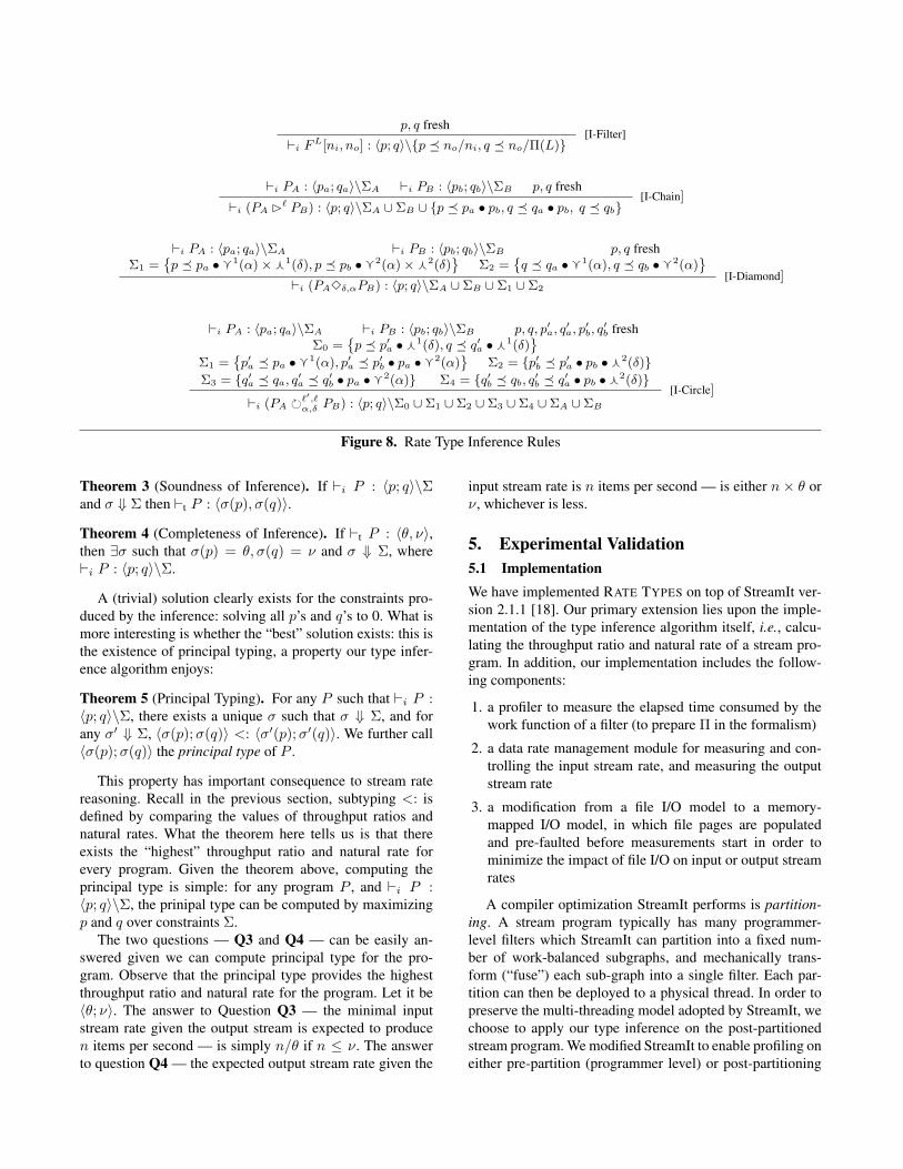
Type inference rules are given in Figure 8. Judgment`i P : 〈p; q〉\Σ says program P is inferred to have through-put ratio represented by type variable p and natural rate rep-resented by type variable q under constraint Σ. The ruleshave a one-to-one correspondence with the type checkingrules we introduced in Figure 6. Indeed, the close relation-ship between the two can be formally established:

p, q fresh

`i FL[ni, no] : 〈p; q〉\{p � no/ni, q � no/Π(L)}[I-Filter]

`i PA : 〈pa; qa〉\ΣA `i PB : 〈pb; qb〉\ΣB p, q fresh

`i (PA �` PB) : 〈p; q〉\ΣA ∪ ΣB ∪ {p � pa • pb, q � qa • pb, q � qb}[I-Chain]

`i PA : 〈pa; qa〉\ΣA `i PB : 〈pb; qb〉\ΣB p, q freshΣ1 =

˘p � pa •g1(α)×f1(δ), p � pb •g2(α)×f2(δ)

¯Σ2 =

˘q � qa •g1(α), q � qb •g2(α)

¯`i (PA3δ,αPB) : 〈p; q〉\ΣA ∪ ΣB ∪ Σ1 ∪ Σ2

[I-Diamond]

`i PA : 〈pa; qa〉\ΣA `i PB : 〈pb; qb〉\ΣB p, q, p′a, q′a, p

′b, q

′b fresh

Σ0 =˘p � p′a •f1(δ), q � q′a •f1(δ)

¯Σ1 =

˘p′a � pa •g1(α), p′a � p′b • pa •g2(α)

¯Σ2 = {p′b � p′a • pb •f2(δ)}

Σ3 = {q′a � qa, q′a � q′b • pa •g2(α)} Σ4 = {q′b � qb, q′b � q′a • pb •f2(δ)}

`i (PA �`′,`α,δ PB) : 〈p; q〉\Σ0 ∪ Σ1 ∪ Σ2 ∪ Σ3 ∪ Σ4 ∪ ΣA ∪ ΣB

[I-Circle]

Figure 8. Rate Type Inference Rules

Theorem 3 (Soundness of Inference). If `i P : 〈p; q〉\Σand σ ⇓ Σ then `t P : 〈σ(p), σ(q)〉.

Theorem 4 (Completeness of Inference). If `t P : 〈θ, ν〉,then ∃σ such that σ(p) = θ, σ(q) = ν and σ ⇓ Σ, where`i P : 〈p; q〉\Σ.

A (trivial) solution clearly exists for the constraints pro-duced by the inference: solving all p’s and q’s to 0. What ismore interesting is whether the “best” solution exists: this isthe existence of principal typing, a property our type infer-ence algorithm enjoys:

Theorem 5 (Principal Typing). For any P such that `i P :〈p; q〉\Σ, there exists a unique σ such that σ ⇓ Σ, and forany σ′ ⇓ Σ, 〈σ(p);σ(q)〉 <: 〈σ′(p);σ′(q)〉. We further call〈σ(p);σ(q)〉 the principal type of P .

This property has important consequence to stream ratereasoning. Recall in the previous section, subtyping <: isdefined by comparing the values of throughput ratios andnatural rates. What the theorem here tells us is that thereexists the “highest” throughput ratio and natural rate forevery program. Given the theorem above, computing theprincipal type is simple: for any program P , and `i P :〈p; q〉\Σ, the prinipal type can be computed by maximizingp and q over constraints Σ.

The two questions — Q3 and Q4 — can be easily an-swered given we can compute principal type for the pro-gram. Observe that the principal type provides the highestthroughput ratio and natural rate for the program. Let it be〈θ; ν〉. The answer to Question Q3 — the minimal inputstream rate given the output stream is expected to producen items per second — is simply n/θ if n ≤ ν. The answerto question Q4 — the expected output stream rate given the

input stream rate is n items per second — is either n× θ orν, whichever is less.

5. Experimental Validation5.1 ImplementationWe have implemented RATE TYPES on top of StreamIt ver-sion 2.1.1 [18]. Our primary extension lies upon the imple-mentation of the type inference algorithm itself, i.e., calcu-lating the throughput ratio and natural rate of a stream pro-gram. In addition, our implementation includes the follow-ing components:

1. a profiler to measure the elapsed time consumed by thework function of a filter (to prepare Π in the formalism)

2. a data rate management module for measuring and con-trolling the input stream rate, and measuring the outputstream rate

3. a modification from a file I/O model to a memory-mapped I/O model, in which file pages are populatedand pre-faulted before measurements start in order tominimize the impact of file I/O on input or output streamrates

A compiler optimization StreamIt performs is partition-ing. A stream program typically has many programmer-level filters which StreamIt can partition into a fixed num-ber of work-balanced subgraphs, and mechanically trans-form (“fuse”) each sub-graph into a single filter. Each par-tition can then be deployed to a physical thread. In order topreserve the multi-threading model adopted by StreamIt, wechoose to apply our type inference on the post-partitionedstream program. We modified StreamIt to enable profiling oneither pre-partition (programmer level) or post-partitioning

(core level) filters. We also ensure each partition is appropri-ately deployed and executed on a unique core. Our experi-ments consider two partitioning scenarios: 8 partitions/coresand 16 partitions/cores.

5.2 Benchmarks and PlatformsOur selection of benchmarks include both micro-benchmarksand a number of existing StreamIt programs [29]. For micro-benchmarking, we focused on demonstrating the effective-ness of reasoning on the four basic stream graph configura-tions:

• TRIV-Filter: a single filter that pops a single valuefor each firing, performs a (parameterized amount of)calculation, and pops a single result

• TRIV-Chain: two TRIV-Filter’s in a chain compo-sition

• TRIV-Diamond: two TRIV-Filter’s in a diamondcomposition

• TRIV-Circle: two TRIV-Filter’s in a circle com-position

The five real-world StreamIt programs we selected are:

• bitonic: an implementation of Batcher’s bitonic sortnetwork for sorting power-of-2 sized key sets

• dct: an implementation of a two-dimensional 8 x 8inverse Discrete Cosine Transfer, which transforms a16 x 16 signal from frequency domain to signal domain

• fft: a streamed implementation of a Fast Fourier Trans-form

• fm: a simulation of an FM radio with a multi-band equal-izer

• vocoder: an implementation of a the speech filter anal-ysis portion of a source-filter model. The analysis in-cludes Fourier analysis, a low-pass filter, a bank of band-pass filters, and a pitch detector

We made minor modifications to these benchmarks, pri-marily to ensure each benchmark reads input data from afile, and writes output data to a file. We equipped our filereader with the capability to provide a constant number ofdata items per second, based on a parameter, to provide acontrollable stream input rate. Our file writer measures thenumber of data items written, and the elapsed time from thefirst to the last write so we can calculate the average streamgraph output rate.

For each benchmark, we perform experiments and re-port results running on two different platforms. The firstwas an 8-core AMD FX-8150 processor (Bulldozer micro-architecture) running Debian 3.2.46-1 Linux (kernel 3.2.0-4-amd64) and 16GB memory. The second was a 32-core AMDOpteron 6378 processor (Piledriver micro-architecture) run-

ning Debian 3.2.46-1 x86-64 Linux (kernel 3.2.0-4-amd64)with 64GB memory.

5.3 Experimental MethodologiesOverall, our experiments for each benchmark are designed todemonstrate the relationship between (1) the throughput ra-tio bound and natural rate bound as computed by our imple-mented type inference algorithm, and (2) the output streamrates measured at various different input stream rates. Forexample, the “throughput ratio bound” line and the “naturalrate bound” line in Figure 1 we showed at the beginning ofthe paper are plotted by applying the type inference algo-rithm on TRIV-Filter. The “measured rate” line in the sameFigure are computed by measuring output stream rates at dif-ferent input stream rates. We now detail several practical is-sues in the experimentation process.

Measurement Point Selection The first issue is to deter-mine the range of input stream rates we wish to measure. Themaximum measurement input rate we benchmark is heuris-tically determined to be the lower of the following two:

• Twice the computed natural rate bound divided by thecomputed throughput ratio bound

• Twice the measured fastest practical output rate di-vided by the computed throughput ratio bound, wherethe fastest practical output rate is measured through a testrun where no restriction is placed on the input stream

We choose 200 measurement points decrementing fromthe maximum measurement input rate down to zero in 200equal steps. In some cases, benchmarks may not reach themaximum measurement input rate due to system-level re-strictions. In these cases, we selected the highest reachableinput rate as maximum measurement input rates.

When given very low input stream rates, the execution ofsome benchmarks may take a long time. We choose to stopmeasurements on a specific benchmark when the executiontime exceeds 5 minutes. Even though we sometimes droppedthe lowest one or two measurement points in some of ourbenchmarks, it had no impact on the trends demonstrated inour results.

Batch Size Selection In a stream program execution, each(post-partition) filter runs in a separate thread, deployed ona separate core. The streams flowing in between filters arethus inter-thread data transfers across cores, via a buffer.This leads to some practical issues: first, there is overheadfor data movement from one core to another, and second,there is a need for synchronization for shared buffer access.To reduce the overhead from data movement and synchro-nization, StreamIt performs batching at data transfer time:an “upstream” filter places a “batch” of data (instead of justone element) in the shared buffer, before it becomes avail-able for consumption by the “downstream” filter.

The effects of this implementation on our experiments aretwofold. On one hand, the effect is similar to the “bursty

behaviors” we described for Theorem 2. Given a long exe-cution where the number of processed data far exceeds thesize of the batch, the “bursty” behavior from batching shouldhave little effect on the average stream rate, and should notaffect our reasoning. On the other hand, the idealized the-oretical model does not consider the data transfer and syn-chronization overhead which will occur in real-world imple-mentations. The selection of batch size in fact has non-trivialeffect on this overhead.

Larger batch sizes (i.e., more data per movement) reducessynchronization overhead, but its bursty nature results indownstream idle time, waiting for a full batch. In somecases, especially for stream graphs with circle constructs,a very large batch size can delay execution of downstreamfilters to the point where the entire stream graph stalls. Largebatch sizes also have the effect of reducing parallel activity.Downstream filters must wait for a full batch before startingexecution. A smaller batch size resolves these problems,but introduces more synchronization overhead, and henceimpacts the ability to achieve theoretical stream rates. Wetuned the batch size for our experiments. All experimentalresults were produced with a batch size of 100 data items.

Overhead and Compensation There are several practicalconsiderations which can cause the measured rates to deviatefrom the theoretical throughput ratio bound and natural ratebound, including the following:

• The idealized model assumes zero time for data transfersacross filters. It further assumes there is no overheadassociated with checking whether there are sufficient dataavailable to invoke a filter.

• The idealized model assumes infinite sized stream buffers,with no overhead for synchronization. In practice, buffersize is fixed, resulting in occasional “back pressure”where a filter must wait for available stream buffer spacein order to push a new data item. There is also lockingand unlocking overhead for synchronizing the transfer ofdata batches.

• There may also be a limit on the fastest rate that an outputstream can be consumed, caused by the mechanics of theoutput stream I/O. In our experiments, the output streamis consumed by memory mapped file output, so is limitedby memory transfer rates.

The impact of these effects are most prominent on filterswhich run very fast. In order to compensate for these effects,we increase the elapsed times for “fast” filters linearly, bya constant compensation ratio. Heuristically, we consider afilter as “fast” if its execution time (per firing) is less than 2microseconds.

We determine the compensation ratio as follows. We firstfind whether the “fast” filter happens to be a “limiting” fil-ter: we consider a filter as limiting if changes in its elapsedtime have direct impact on the output stream rate of the en-tire program. We find limiting filters by re-calculating the

theoretical output rate under the assumption that the filter inquestion has a higher natural rate and determining if such achange would lead the type inference algorithm to compute adifferent output rate. Second, for each filter that is both “fast”and “limiting,” we plot an (x, y) point in a graph where x isthe natural rate (computed through the inverse of the pro-filed elapsed time), and y is the observed data production/-consumption rate, obtained through monitoring the changesin low-level data buffers, both in units of “1/microsecond.”Third, a linear regression is performed to determine the con-stant compensation ratio. As expected, the compensation ra-tio differs from platform to platform, depending factors suchas inter-core latency. Our linear regression resulted in the fit-ting functions y = x×0.686+0.028 on the 8-core machine,and y = x × 1.6734 + 0.045 on the 32-core machine. Ourcompensation only affects filters that are both fast and limit-ing.

5.4 Experimental ResultsDetailed experimental results are in Figure 9. The results ofmicro-benchmarks are demonstrated in Figures 9(a)(b)(c)(d),and the results for StreamIt benchmarks are in the rest of theFigures. Overall, we believe the results experimentally con-firm the effectiveness of our reasoning framework.

Microbenchmarking — Figures 9(a)(b)(c)(d) — showsvery close resemblance between the theoretical result andthe measured result: observe that the (blue) solid line liesalmost exactly on the boundaries carved out by the two dot-ted lines. Since micro-benchmarks all have less than 8 fil-ters, the results on both the 8-core machine and the 32-coremachine are similar, and we only present the 8-core ver-sion. Relatively speaking, TRIV-Circle (and to some extentTRIV-Diamond) experiences more frequent fluctuations, asshown in Figures 9(c)(d). This phenomenon also recurs inreal-world StreamIt benchmarks with the same compositionoperators. Recall that both forms of compositions involveforking and joining of streams. We speculate the fluctuationis related to the behaviors of forking and joining, especiallyin the presence of batching.

For StreamIt benchmarks, Figures 9(e)(f)(g)(h)(i) showthe results when the benchmarks are partitioned into 8partitions and run on the 8-core machine, whereas Fig-ures 9(j)(k)(l)(m)(n) are their counterparts while being par-titioned into 16 partitions and run on the 32-core machine.Even though the 32-core machine has a higher level of par-allelism, the 8-core machine runs at a higher frequency (3.6GhZ) than the 32-core machine (2.4 GhZ), so the outputstream rates were typically higher for the 8-core versions. Inmost cases — the exceptions are perhaps the two vocoderbenchmark results — the measured rates still closely fit thetheoretical results from type inference. For the fm bench-mark, its 8-core execution is unable to consume more than25,000 items per second due to I/O restrictions, so we areunable to select the measurement points far to the right onthe X-axis, as demonstrated in Figure 9(h). We discussed

(a) TRIV-Filter (e) bitonic - 8 filter (j) bitonic - 16 filter

(b) TRIV-Chain (f) dct - 8 filter (k) dct - 16 filter

(c) TRIV-Diamond (g) fft - 8 filter (l) fft - 16 filter

(d) TRIV-Circle (h) fm - 8 filter (m) fm - 16 filter

(i) vocoder - 8 filter (n) vocoder - 16 filter

Figure 9. Benchmark Results (X axis: input stream rate in 1000 items/second; Y axis: output stream rate in 1000 items/second)

this issue in the “measurement point selection” subsection.Note that this issue goes away for its 16-core execution inFigure 9(m). The converse is true for the dct benchmark,which runs at all input rates for the 8-core execution, but islimited for the 16-core execution.

The least satisfying results are from the vocoder bench-mark, in Figures 9(i)(n). We investigated the runtime of thisbenchmark, and found that the filter that limits the over-all output rate is being fed by a very high volume of inputstream data as compared with the other benchmarks. On the16-core version, this filter has 7.5M data items per secondavailable, but can only consume 2.3M data items per second.The computed natural rate says it should be able to consume2.9M data items per second. We surmise that the high streamdata rates incur a higher batching and synchronization coststhan expected.

6. Generality and LimitationsIn this section, we place RATE TYPES in a broader contextby evaluating the potential opportunities and limitations ofbuilding a similar type system on top of several data-orientedprogramming languages other than our current implementa-tion. Our intent is to examine the generality of RATE TYPESby probing how syntactic, semantic, and implementationchoices made by RATE TYPES impact its applicability.

Table 1 summarizes our investigation, where each rowcharacterizes a representative data-oriented programminglanguage based on columns that delineate syntactic or se-mantic design choices of RATE TYPES. These design choicesare:

• Synchronous Input - characterizes the filter firing mecha-nism where filter execution is triggered by the existenceof sufficient input data items for an instance of filter exe-cution.

• Static Items per Firing - identifies the design feature inwhich the number of data items a filter will consumeand produce for each instance of execution is staticallyknown.

• Non-Blocking Memory Access - indicates whether mem-ory access within a filter execution is block-free, i.e.,without waits or locks.

• Graph Composition - explores whether the Chain, Dia-mond, Circle operators that RATE TYPES supports aresufficient to capture the stream graph composition mech-anisms associated with the language.

The languages we investigated, including several lan-guages not traditionally branded as “stream” languages,are selected from a variety of sources from recent liter-ature. The Category column groups these languages intocategories. The “stream” category is closest to our con-text, where high-volume, high-throughput, potentially in-finite data flow through program-defined data processing

units and data paths. The “signal” category is historicallyused in contexts where continuous signals flow throughprogram-defined processing units and paths. Both streamlanguages and signal languages belong to the broader cat-egory of dataflow languages — those characterized by theinvocation of functional units based on the presence of in-put data, rather than an imperative control flow. In dataflowlanguages, data flow through program-defined data process-ing units and data paths, even though data items might befinite, and their volume and throughput may or may not behigh. Toward the end of Section 2, we described why signalor dataflow languages may potentially benefit from RATETYPES.

We next describe the design choices in more detail in or-der to assess their impact on the generality of RATE TYPES.

Impacts of Semantic Choices on Generality Two basic re-quirements of synchronous dataflow (SDF) languages areSynchronous Input and Static Items per Firing. Many lan-guages we studied have not been categorized in the literatureas SDF languages, but as Table 1 shows, most support thesetwo basic semantic requirements.

In most cases, data processing units (i.e., filters in RATETYPES) are modeled as functions, and data read from theinput stream are modeled as function parameters. Further-more, these languages have no capability to access input datastreams other than through parameters. The RATE TYPESSynchronous Input requirement is trivially satisfied by acombination of these two factors. The requirement of StaticItems per Firing is also satisfied thanks to the function-basedfilter design. Most languages align the per-firing input dataitems and the output data items with function parameters andreturn values, whose sizes are statically known through func-tion signatures.

The notable exception is StreamFlex, where input/out-put streams are first-class values (called channels) within thescope of filters. Data stream read is a first-class expressionin StreamFlex, and hence in the most general interpretationof StreamFlex, a programmer can both determine when datashould be read from the input stream, and how many dataitems can be read. In addition, StreamFlex allows program-mers to circumvent the default synchronous input filter fir-ing mechanism by overriding a method called trigger. RATETYPES in its current form cannot support this flexible de-sign. It can be applied in limited cases where the defaulttrigger mechanism is used, and static analysis can determinethe number of channel reads/writes per-firing (e.g., when thedata stream read/write are not in recursions or loops). Theexamples used in the Streamflex paper appear to fit into thesecases.

The majority of the reasoning ability of RATE TYPES —such as the ability to determine the overall data throughputwhen the characteristics of (base case) filters are known —remains intact even when Static Items per Firing does nothold. The primary limitation in a scenario like StreamFlex

Synchronous Static Items Non-Blocking GraphLanguage Category Input per Firing Memory Access Composition

StreamIt [18] stream Yes Yes Yes, except teleporting Chain/Diamond/CircleAurora [3] stream Yes Yes Yes Chain/Diamond

Borealis [30] stream Yes Yes Yes Chain/DiamondSTREAM [31] stream Yes Yes Yes Chain/Diamond

StreamFlex [22] stream No No Yes declarative channelsElm [5] signal Yes Yes Yes function application

FlapJax [32] signal Yes Yes Yes function applicationPig Latin [33] dataflow Yes Yes Yes Chain/DiamondEon/Flux [7] dataflow Yes Yes Yes Chain/Diamond

FlumeJava [25] dataflow Yes Yes Yes Chain/DiamondBamboo [34] dataflow Yes Yes transactional locking typestate-based

Table 1. RATE TYPES Generality and Limitations

lies in when the characteristics of the filters — the leaf nodesin a type derivation — can be known. In the future, we areinterested in developing a dynamic variant of RATE TYPESthat uses lightweight dynamic constraint solving for adaptivestream rate control. We speculate the dynamic variant maybe more suitable for coping with flexible models where thenumber of input/output items per firing fluctuates at runtime.

The Non-Blocking Memory Access column describes thememory access semantics of each language in the presenceof concurrency. RATE TYPES does not place restrictions perse on memory access, but blocking during filter executionmay impact a practical aspect of RATE TYPES: the stabilityof profiling results. Most data-oriented programming mod-els — especially those geared towards high data throughput— either prevent or minimize blocking at the language level,or caution against their common use. The former approach istaken by both languages with a functional core (such as Elmand FlapJax) and languages such as StreamFlex. Indeed, akey design goal of StreamFlex is to implement non-blockingsemantics during filter execution, achieved through a combi-nation of techniques including an ownership type system toreason about memory disjointness, a non-blocking boundedchannel design, and preemptible atomic regions for Javacompatibility. Other languages minimize blocking, such asStreamIt, which defers most blocking needs to an uncom-mon message teleporting mechanism.

The exception here is Bamboo, a language where dataprocessing units (called tasks) can access global memoryand the language enforces atomicity through locks. Bambooacquires all locks required for transactional task executionat the beginning of the task execution. In that sense, non-blocking memory access is still maintained in Bamboo, goodnews for profiling stability. The challenge of applying RATETYPES to Bamboo however is that task firing may not besolely dependent on input data availability, but also lock ac-quisition. Bamboo has a data-oriented programming model,

but its focus is on parallelism support and task scheduling,not stream-like data processing.

Impacts of Syntactic Choices on Generality The GraphComposition column addresses the syntactic choices used tocreate the stream graph common to stream/signal/dataflowprograms: a directed graph in which processing units arenodes and data streams are edges between nodes.

A significant number of languages we studied only al-low acyclic dataflow/stream graphs, a design choice on parwith languages that support Chain and Diamond combina-tors. The scope RATE TYPES considers is more expressive,because it also considers feedbacks. Indeed, the concretegrammar of different languages to construct dataflow/streamgraphs can be diverse, sometimes through algebraic combi-nators like what RATE TYPES uses, or through conventionalnode / edge representations, or simply through a sequence ofassignments (such as in Pig Latin). The difference, however,is largely stylistic, in that though the combinator-based ex-pressions are more friendly for formalization, different syn-tactic styles can be transformed from one to another stati-cally.

In terms of the dataflow graph topology, the flexiblelanguages are StreamFlex, Elm, FlapJax, and Bamboo. InStreamFlex, a filter can declare the channels it interacts with,and the topology of the underlying stream graph may in-volve cycles. Interestingly, since the channels in StreamFlexmust be explicitly declared for each filter, the stream graphcan be statically inferred through a trivial program analy-sis. We speculate RATE TYPES can be applied when thestatic stream graph (which may or may not contain cycles)is known. Elm and FlapJax follow the tradition of FRP lan-guages, where function composition – when two functionswhich take a stream as an argument and produce a streamas a result are composed — can be viewed analogously asa form of Chain, and the typing rule for Chain of RATETYPES can be built analogously for function compositionexpressions. Notably, most signal languages come up withwell-defined combinators, which match well with the syn-

tactic choices of RATE TYPES. For example, mergeE inFlapJax is similar to the joining of Diamond.

Bamboo adopts a syntax conceptually related to tuplespaces, where (in the view of programmers) data live in theglobal space. A Bamboo programmer defines tasks, each ofwhich specifies the types of data (streams) it reads from theglobal space as input and the conditions associated with thatstream to fire the task. Once fired, the task processes the dataitem and places the processed item back to the global space.Since all streams are strongly typed and the conditions aredeclarative similar to typestates, we speculate the task/datadependency explicitly declared in Bamboo programs mayhelp induce the stream graph. Interestingly, Bamboo’s com-piler infers a combined state transition graph for optimiza-tion purposes. This data structure explicitly expresses thedata flows between tasks, which appears to be a refined formof stream graphs.

An orthogonal issue is the expressiveness of the streammanipulation operators themselves. For instance, FlumeJavasupports the groupByKeys operator to compute equiva-lence classes for a finite set of data items, and Pig Latinsupports operators to compute the cross product of multi-ple finite streams, such as the COGROUP operator. To in-vestigate the applicability of RATE TYPES in these cases,there are two separate issues: (1) whether such operatorscan be encoded through the primitives currently in RATETYPES; (2) whether the program analysis enabled by RATETYPES can precisely predict performance over the encod-ings of such operators. We believe (1) can be answered pos-itively (see Appendix), but the answer to (2) relies on howfaithful the encodings are to the internal implementation ofthese operators. For practical adoption of RATE TYPES tothese languages, the more direct route is to consider theseoperators as language primitives, a direction open for fur-ther research. This incompleteness should come as no sur-prise: RATE TYPES considers the more general case of dataprocessing over dataflow graphs, whereas languages such asFlumeJava and Pig Latin further refine/restrict the domain byfocusing on database programming with finite-sized tables.

Finally, even though unseen in formalisms, practical lan-guages often allow multiple output streams, and sometimesmultiple input streams for increased programmability. Inthese cases, RATE TYPES can be extended in a predictablemanner to construct constraints for each of the input/outputstreams independently. In the inference algorithm, each in-put/output stream should be represented by a separate ratetype variable.

Impacts of Implementation Choices on Generality Ourimplementation base, StreamIt, is a relatively optimizedstreaming infrastructure. It should be pointed out however,the effectiveness of RATE TYPES reasoning in practice –such as predicting the throughput of a stream program –is largely orthogonal to whether the base infrastructure ishighly optimized or not. The key insight here is that RATE

TYPES reasoning can be effective as long as the overheadintroduced by the base stream infrastructure can be well ac-counted for. Stream processing overhead can be divided intotwo categories: a small fixed overhead required per firing,and an often larger overhead proportional to the idle timeassociated with a filter, such as the time required for polling.The overhead proportional to idle time does not affect streamrates because it consumes idle time, not the time required toproduce output data. The remaining fixed, per-firing over-head will reduce the output rate only when the per-firingoverhead far exceeds that due to the idle time of a filter. Aslong as the per-firing overhead is sufficiently compensated inthe inference, RATE TYPES will guide real-world systems toproduce experimental results with accuracy. Indeed, even ina relatively optimized system such as StreamIt, the overheadstill needs to be compensated, in a fashion we described inSection 5, and we believe similar overhead compensationstrategies can be constructed for other streaming languagesystems, no matter what level of optimization is present.

Our implementation of RATE TYPES on top of theStreamIt infrastructure interacts with three important fea-tures of StreamIt, namely profiling, partitioning, and streambatching. Among them, only StreamIt’s profiling feature is a“helper” to our implementation, and the other two features infact complicated our implementation as we described in Sec-tion 5. Take partitioning for instance, the feature that refac-tors the stream graph so that the number of filters matchesthe number of cores available on the hardware. Since ouroperational semantics considers each filter as a separatethread, we have to take StreamIt’s partitioning into consid-eration and work with its post-partition graph. The StreamItstream batching feature required significant tuning for RATETYPES, as discussed in the Batch Size Selection paragraph insection 5. We used StreamIt’s profiler only after significantmodification, and surmise that similar modifications couldenable similar capabilities in other languages.

7. Related WorkStream languages have their root in dataflow languages.Earlier examples include Lucid [35], LUSTRE [36], andPtolemy [21], with well-known foundations such as Kahnnetworks [37]. Among them, the operational semantics ofRATE TYPES is closest to the synchronous dataflow (SDF)design of Ptolemy, which later influenced the design ofStreamIt, the system our implementation is built upon. Aclassic static reasoning result on SDF is static scheduling,by Lee and Messerschmitt [16]. The goal of static schedul-ing is to compute a schedule, e.g., AAB to mean filter Ashould be fired twice for every filter B execution. This al-gorithm is influential in the design of stream languages. Forinstance, StreamIt adopts a variant of the algorithm, calledsteady-state scheduling [23]. Our type system is orthogo-nal to static scheduling, both in goals and in methodologies.RATE TYPES finds the best possible output rate, independent

of the firing order of the filters. A good schedule will comeclose to achieving the best possible rate, but even the bestpossible schedule cannot exceed that limit. RATE TYPES isa type-based compositional reasoning framework, whereasLee and Messerschmit is based on graph theory through anotion called a topology matrix.

Clock calculus [17] is based on a restrictive form ofSDF, where different sub-programs (filters) of a stream pro-gram are synchronized. Their type system infers a “clock”to synchronize filters. RATE TYPES does not require anysynchronization between sub-programs. Furthermore, un-like clock calculus where filter execution time is treatedas “unit length,” RATE TYPES illuminates the relationshipbetween filter execution time and stream rates. Thiele andStoimenov [38] studied performance analysis in the presenceof cycles in SDF. They do not define a dynamic semantics toformally relate the runtime and the analysis, and their ap-proach is not type-based.

Some type systems exist to reason about non-quantitativeaspects of stream/dataflow/signal programs. StreamFlex [22]has an ownership type system aimed at enforcing memorysafety, especially non-shared memory access from differ-ent filters. A dependent type system [39] was designed forFRP to enforce productivity: a liveness property to guaran-tee the program continues to deliver output. Krishnaswamiet al. [40] introduced a linear type system to bound resourceusage (especially space) in higher-order FRP. Suenaga etal. [11] designed a type system in the Hoare-style on topof a stream language core as an example to demonstrate theexpressiveness of their discrete-continuous transfer frame-work for verification. Elm [5] as a FRP-family language hasa type system to outlaw higher-order signals. None of the re-lated work above reasons about the rate of data processing.

For control-flow languages, there is a large body of workon qualitative and quantitative reasoning of performance-related properties, e.g., WCET [12], cost semantics [13],resource usage analysis [14], amortized resource analysis[15], and Energy Types [41]. RATE TYPES focuses on thedata rates of data-flow programming models.

Our prior work Green Streams [42] achieves energy ef-ficiency by DVFS through a program analysis on balancingdata rates. The analysis is not type-based, and with a differ-ent goal. The two systems share the high-level observationin analyzing stream programs: data rates can be abstracted.

8. ConclusionThis paper describes a novel type system for performancereasoning over stream programs, focusing on a highly dy-namic aspect – stream rate control. Our experimental resultsshow the reasoning framework can effectively predict streamprogram behaviors in terms of data throughput.

The proofs of theorems and lemmas described in the pa-per can be found in the accompanying technical report [28].

Acknowledgments We thank the anonymous reviewers fortheir useful suggestions, and Amer Diwan and Jens Palsbergfor insightful discussions. This work is partially supportedby NSF CCF-1054515. Any opinions expressed here arefrom the authors and do not necessarily reflect the views ofthe sponsors.

References[1] Thies, W., Amarasinghe, S.: An empirical characterization

of stream programs and its implications for language andcompiler design. In: PACT ’10. (2010) 365–376

[2] Nvidia: Compute unified device architecture programmingguide. NVIDIA: Santa Clara, CA (2007)

[3] Carney, D., Cetintemel, U., Cherniack, M., Convey, C., Lee,S., Seidman, G., Stonebraker, M., Tatbul, N., Zdonik, S.B.:Monitoring streams - a new class of data management appli-cations. In: VLDB. (2002) 215–226

[4] Krishnaswami, N.R., Benton, N.: A semantic model forgraphical user interfaces. In: ICFP ’11. (2011) 45–57

[5] Czaplicki, E., Chong, S.: Asynchronous functional reactiveprogramming for GUIs. In: PLDI’13. (June 2013)

[6] Elliott, C., Hudak, P.: Functional reactive animation. In: ICFP’97. (1997) 263–273

[7] Sorber, J., Kostadinov, A., Garber, M., Brennan, M., Corner,M.D., Berger, E.D.: Eon: a language and runtime system forperpetual systems. In: SenSys ’07. (2007) 161–174

[8] Monsanto, C., Foster, N., Harrison, R., Walker, D.: A compilerand run-time system for network programming languages. In:POPL ’12. (2012) 217–230

[9] Soule, R., Hirzel, M., Grimm, R., Gedik, B., Andrade, H., Ku-mar, V., Wu, K.L.: A universal calculus for stream processinglanguages. In: ESOP’10. (2010) 507–528

[10] Botincan, M., Babic, D.: Sigma*: symbolic learning of input-output specifications. In: POPL ’13. (2013) 443–456

[11] Suenaga, K., Sekine, H., Hasuo, I.: Hyperstream processingsystems: nonstandard modeling of continuous-time signals.In: POPL ’13. (2013) 417–430

[12] Wilhelm, R., Engblom, J., Ermedahl, A., Holsti, N., Thesing,S., Whalley, D., Bernat, G., Ferdinand, C., Heckmann, R., Mi-tra, T., Mueller, F., Puaut, I., Puschner, P., Staschulat, J., Sten-strom, P.: The worst-case execution-time problem – overviewof methods and survey of tools. ACM Trans. Embed. Comput.Syst. 7(3) (May 2008) 36:1–36:53

[13] Blelloch, G.E., Greiner, J.: A provable time and space efficientimplementation of nesl. In: ICFP ’96. (1996) 213–225

[14] Igarashi, A., Kobayashi, N.: Resource usage analysis. In:POPL ’02. (2002) 331–342

[15] Hoffmann, J., Aehlig, K., Hofmann, M.: Multivariate amor-tized resource analysis. In: POPL ’11. (2011) 357–370

[16] Lee, E.A., Messerschmitt, D.G.: Static scheduling of syn-chronous data flow programs for digital signal processing.IEEE Trans. Comput. 36(1) (January 1987) 24–35

[17] Cohen, A., Duranton, M., Eisenbeis, C., Pagetti, C., Plateau,F., Pouzet, M.: N-synchronous kahn networks: a relaxed

model of synchrony for real-time systems. In: POPL ’06.(2006) 180–193

[18] Thies, W., Karczmarek, M., Amarasinghe, S.P.: StreamIt: Alanguage for streaming applications. In: CC’02. (2002) 179–196

[19] Kirkpatrick, S., Gelatt, C.D., Vecchi, M.P.: Optimization bysimulated annealing. Science 220 (1983) 671–680

[20] Agha, G.: ACTORS : A model of Concurrent computationsin Distributed Systems. MITP, Cambridge, Mass. (1990)

[21] Lee, E., Messerschmitt, D.: Synchronous data flow. Proceed-ings of the IEEE 75(9) (Sept 1987) 1235–1245

[22] Spring, J.H., Privat, J., Guerraoui, R., Vitek, J.: StreamFlex:high-throughput stream programming in Java. In: OOPSLA’07. (2007) 211–228

[23] Gordon, M.I., Thies, W., Amarasinghe, S.: Exploiting coarse-grained task, data, and pipeline parallelism in stream pro-grams. In: ASPLOS’06. (2006)

[24] Furr, M., An, J.h.D., Foster, J.S.: Profile-guided static typingfor dynamic scripting languages. In: OOPSLA ’09. (2009)283–300

[25] Chambers, C., Raniwala, A., Perry, F., Adams, S., Henry,R.R., Bradshaw, R., Weizenbaum, N.: FlumeJava: easy, ef-ficient data-parallel pipelines. In: PLDI ’10. (2010) 363–375

[26] Morton, K., Balazinska, M., Grossman, D.: ParaTimer: aprogress indicator for MapReduce DAGs. In: SIGMOD ’10.(2010) 507–518

[27] Bohannon, A., Foster, J.N., Pierce, B.C., Pilkiewicz, A.,Schmitt, A.: Boomerang: resourceful lenses for string data.In: POPL ’08. (2008) 407–419

[28] Bartenstein, T., Liu, Y.D.: Rate Types for Stream Programs- Technical Report. https://www.cs.binghamton.edu/˜tbarten1/RateTypesForStreamPrograms_TechReport.pdf, (2014)

[29] Gordon, M.I.: Compiler Techniques for Scalable Performanceof Stream Programs on Multicore Architectures. PhD thesis,Massachusetts Institute of Technology, Cambridge, MA (May2010)

[30] Abadi, D.J., Ahmad, Y., Balazinska, M., Cetintemel, U., Cher-niack, M., Hwang, J.H., Lindner, W., Maskey, A., Rasin, A.,Ryvkina, E., et al.: The design of the borealis stream process-ing engine. In: CIDR. Volume 5. (2005) 277–289

[31] Motwani, R., Widom, J., Arasu, A., Babcock, B., Babu, S.,Datar, M., Manku, G., Olston, C., Rosenstein, J., Varma, R.:Query processing, resource management, and approximationin a data stream management system, CIDR (2003)

[32] Meyerovich, L.A., Guha, A., Baskin, J., Cooper, G.H., Green-berg, M., Bromfield, A., Krishnamurthi, S.: Flapjax: a pro-gramming language for Ajax applications. In: OOPSLA ’09.(2009) 1–20

[33] Olston, C., Reed, B., Srivastava, U., Kumar, R., Tomkins, A.:Pig latin: A not-so-foreign language for data processing. In:Proceedings of the 2008 ACM SIGMOD International Con-ference on Management of Data. SIGMOD ’08, New York,NY, USA, ACM (2008) 1099–1110

[34] Zhou, J., Demsky, B.: Bamboo: a data-centric, object-orientedapproach to many-core software. In: PLDI’10, ACM (2010)388–399

[35] Ashcroft, E.A., Wadge, W.W.: Lucid, a nonprocedural lan-guage with iteration. Commun. ACM 20(7) (July 1977)

[36] Caspi, P., Pilaud, D., Halbwachs, N., Plaice, J.A.: LUSTRE:a declarative language for real-time programming. In: POPL’87. (1987) 178–188

[37] Kahn, G.: The semantics of a simple language for parallelprogramming. In Rosenfeld, J.L., ed.: Information processing,Stockholm, Sweden, North Holland, Amsterdam (Aug 1974)471–475

[38] Thiele, L., Stoimenov, N.: Modular Performance Analysis ofCyclic Dataflow Graphs. In: Proceedings of the Seventh ACMInternational Conference on Embedded Software. EMSOFT’09, New York, NY, USA, ACM (2009) 127–136

[39] Sculthorpe, N., Nilsson, H.: Safe functional reactive program-ming through dependent types. In: ICFP ’09. (2009) 23–34

[40] Krishnaswami, N.R., Benton, N., Hoffmann, J.: Higher-orderfunctional reactive programming in bounded space. In: POPL’12. (2012) 45–58

[41] Cohen, M., Zhu, H.S., Emgin, S.E., Liu, Y.D.: Energy types.In: OOPSLA ’12. (October 2012)

[42] Bartenstein, T., Liu, Y.D.: Green streams for data-intensivesoftware. In: ICSE’13. (May 2013)

AppendixA. EncodingFirst, a k-way fork-join of programs P1, . . . , Pk with dis-tribution factor δ = 〈n1; . . . ;nk〉 and aggregation factorα = 〈n′1; . . . ;n′k〉 can be encoded as:

P13δ1,α1(P23δ2,α2(. . . (Pk−13δn−1,αn−1Pk)))

where δi = 〈ni;ni+1 + . . .+nk〉 and αi = 〈n′i;n′i+1 + . . .+n′k〉 for i = 1..n− 1.

Round-robin is not the only way the input stream of asplit-join can be divided. Another useful pattern is to du-plicate every input stream element, and feed each dupli-cate to the input stream of the two sub-programs (say P1

and P2) participating the split-join. This can be encoded asFL[1, 2]�(P13〈1;1〉,αP2) where F is function that takes [x]and returns [x, x] with Π(L) = 0.

Similarly, the output stream of a split-join does not needto be aggregated through round-robin either. A useful pat-tern is to aggregate the two output streams of the two sub-programs (say P1 and P2) participating the split-join throughsome binary operators. For example, one may wish to onlyput the greater value of each pair of output elements of P1

and P2 to the output stream of the split-join. This can be en-coded as (P13δ,〈1;1〉P2) � FL[2, 1] where F represents thebinary operator. For the example above, F is the functionthat takes [x, y] and returns [max(x, y)] where max () is thestandard maximum operator.

In a streaming database query language, a database tablejoin operation typically consists of a cross-product of a finitewindow over two input streams. Such a cross product can bemodeled with a round-robin join, followed by a filter whichpops a full window’s worth of input data, and then pushesthe cross-product of that window.

Last, our formal system idealizes the data transfer acrossbuffers. Consider the chain composition P1�P2 for instance.

A real-world implementation would place a buffer betweenthe output stream of P1 and the input stream of P2. Suchbuffer read/write may take time. The time of buffer read-/write can accounted for by encoding P1 � FL[1, 1] � P2

whereF is the identity function, and Π(L) is the time neededfor buffer access.