Rate of Erosion Properties of Rock and Clay€¦ · Final Report Rate of Erosion Properties of Rock...

Final Report

Rate of Erosion Properties of Rock and Clay (CORRELATION OF EROSION RATE-SHEAR STRESS RELATIONSHIPS WITH

GEOTECHNICAL PROPERTIES OF ROCK AND COHESIVE SEDIMENTS)

BD-545, RPWO # 3 UF Project 00030890 (4554013-12)

Submitted by:

D. Max Sheppard David Bloomquist Philip M. Slagle

Department of Civil and Coastal Engineering

University of Florida Gainesville, Florida 32611

Developed for the

Rick Renna, P.E., Project Manager December, 2006

ii

Disclaimer

The opinions, findings, and conclusions expressed in this publication are those of the

author and not necessarily those of the State of Florida Department of Transportation.

SI (MODERN METRIC) CONVERSION FACTORS (from FHWA)

APPROXIMATE CONVERSIONS TO SI UNITS

SYMBOL WHEN YOU KNOW MULTIPLY BY TO FIND SYMBOL LENGTH

in inches 25.4 millimeters mm ft feet 0.305 meters m yd yards 0.914 meters m mi miles 1.61 kilometers km

SYMBOL

WHEN YOU KNOW MULTIPLY BY TO FIND SYMBOL

AREA in2 squareinches 645.2 square millimeters mm2 ft2 squarefeet 0.093 square meters m2 yd2 square yard 0.836 square meters m2 ac acres 0.405 hectares ha

mi2 square miles 2.59 square kilometers km2

SYMBOL WHEN YOU KNOW MULTIPLY BY TO FIND SYMBOL

VOLUME fl oz fluid ounces 29.57 milliliters mL gal gallons 3.785 liters L ft3 cubic feet 0.028 cubic meters m3 yd3 cubic yards 0.765 cubic meters m3

NOTE: volumes greater than 1000 L shall be shown in m3


MASS oz ounces 28.35 grams g lb pounds 0.454 kilograms kg T short tons (2000 lb) 0.907 megagrams (or

"metric ton") Mg (or "t")

SYMBOL


TEMPERATURE (exact degrees) oF Fahrenheit 5 (F-32)/9

or (F-32)/1.8 Celsius oC

SYMBOL


ILLUMINATION fc foot-candles 10.76 lux lx fl foot-Lamberts 3.426 candela/m2 cd/m2


FORCE and PRESSURE or STRESS lbf poundforce 4.45 newtons N

lbf/in2 poundforce per square inch 6.89 kilopascals kPa

ii

APPROXIMATE CONVERSIONS TO ENGLISH UNITS

SYMBOL WHEN YOU KNOW MULTIPLY BY TO FIND SYMBOL LENGTH

mm millimeters 0.039 inches in m meters 3.28 feet ft m meters 1.09 yards yd

km kilometers 0.621 miles mi


AREA mm2 square millimeters 0.0016 square inches in2 m2 square meters 10.764 square feet ft2 m2 square meters 1.195 square yards yd2 ha hectares 2.47 acres ac

km2 square kilometers 0.386 square miles mi2


VOLUME mL milliliters 0.034 fluid ounces fl oz L liters 0.264 gallons gal m3 cubic meters 35.314 cubic feet ft3 m3 cubic meters 1.307 cubic yards yd3

SYMBOL WHEN YOU KNOW MULTIPLY BY TO FIND SYMBOL MASS

g grams 0.035 ounces oz kg kilograms 2.202 pounds lb

Mg (or "t") megagrams (or "metric ton")

1.103 short tons (2000 lb) T

SYMBOL


TEMPERATURE (exact degrees) oC Celsius 1.8C+32 Fahrenheit oF


ILLUMINATION lx lux 0.0929 foot-candles fc

cd/m2 candela/m2 0.2919 foot-Lamberts fl


FORCE and PRESSURE or STRESS N newtons 0.225 poundforce lbf

kPa kilopascals 0.145 poundforce per square inch

lbf/in2

*SI is the symbol for the International System of Units. Appropriate rounding

should be made to comply with Section 4 of ASTM E380.(Revised March 2003)

Technical Report Documentation Page

1. Report No.

2. Government Accession No.

3. Recipient's Catalog No.

4. Title and Subtitle

Rate of Erosion Properties of Rock and Clay

(CORRELATION OF EROSION RATE-SHEAR STRESS RELATIONSHIPS WITH

GEOTECHNICAL PROPERTIES OF ROCK AND COHESIVE SEDIMENTS)

BD-545, RPWO # 3

UF Project 00030890 (4554013-12)

5. Report Date December 2006

6. Performing Organization Code

7. Author(s) D. Max Sheppard, David Bloomquist , Philip Slagle

8. Performing Organization Report No.

9. Performing Organization Name and Address Department of Civil and Coastal Engineering

365 Weil Hall University of Florida

Gainesville, Florida 32611

10. Work Unit No. (TRAIS)

11. Contract or Grant No. BC-545, RPWO #3

12. Sponsoring Agency Name and Address

Florida Department of Transportation 605 Suwannee Street, MS 30

Tallahassee, FL 32399

13. Type of Report and Period Covered

Final Report 8/2003 – 10/2006

14. Sponsoring Agency Code 15. Supplementary Notes

16. Abstract Two novel instruments have been designed for testing the erosional characteristics of rock and clay. Results show good agreement in the rate of erosion and the cohesive

strength of rock. Critical shear stress numerical formulations are also provided. 17. Key Word

Erosion, laboratory testing, flume 18. Distribution Statement

No restrictions.

19. Security Classif. (of this report) Unclassified.

20. Security Classif. (of this page)

Unclassified.

21. No. of Pages 102

22. Price

ii

TABLE OF CONTENTS Section Page

TABLE OF CONTENTS .................................................................................................... ii

LIST OF FIGURES ........................................................................................................... iv

LIST OF TABLES ............................................................................................................. vi

Executive Summary .......................................................................................................... vii

CHAPTER 1 INTRODUCTION ............................................................................. 1 1.1 Definition of Bridge Scour.................................................................................1 1.2 Hydrodynamic Analysis of Local Scour ............................................................3 1.3 Need for Research Verification .........................................................................6 1.4 Research Objectives ...........................................................................................7

1.4.1 Purpose .........................................................................................................7

CHAPTER 2 BACKGROUND AND LITERATURE REVIEW ........................... 9 2.1 Rock Description and Scour Behavior ...............................................................9 2.2 Approaches to Estimating Rock Scour Prior to Design ...................................10 2.3 Cohesive Strength of Limestone ......................................................................12 2.4 Cohesive Sediment Description and Scour Behavior ......................................12 2.5 Methodologies to Estimate Cohesive Sediment Scour Prior to Design ...........14 2.6 Local Scour Research in Non-Cohesive Sediments .........................................16 2.7 Previous Flume Studies of Rock and Cohesive Sediment Scour .....................18

2.7.1 Erosion Function Apparatus (EFA) ...........................................................18 2.7.2 Sediment Erosion at Depth Flume (SEDflume) .........................................19 2.7.3 Adjustable Shear Stress Erosion and Transport Flume (ASSET) ..............19

2.8 Scour in Sediment Mixtures .............................................................................20

CHAPTER 3 REVIEW AND UPDATE TO THE EROSION RATE LABORATORY APPARATUSES ......................................................................... 25

3.1 Rotating Erosion Testing Apparatus (RETA) ..................................................25 3.1.1 Description .................................................................................................25 3.1.2 Testing........................................................................................................27

3.2 Sediment Erosion Rate Flume (SERF) ............................................................29 3.2.1 Equipment Description and Developments ...............................................29 3.2.2 Computerized Control Description and Updates .......................................33 3.2.3 Overview of the Testing Procedure ...........................................................36 3.2.4 Data Analysis .............................................................................................37

CHAPTER 4 DESCRIPTION OF EXPERIMENTS ............................................. 38 4.1 Erosion of Uniform Sand .................................................................................38 4.2 Comparison of Natural Limestone Erosion Rates with Cohesive

Strength ............................................................................................................39 4.3 RETA and SERF Tests with Sediment Samples Produced in the

Laboratory ........................................................................................................39

iii

4.3.1 Background ................................................................................................39 4.3.2 Description of Cemented Sand Erosion Tests ...........................................47

4.4 Erosion of Sand-Clay Mixtures .......................................................................50 4.4.1 Sample Preparation for Clay-Sand Mixtures .............................................51

CHAPTER 5 EXPERIMENTAL RESULTS......................................................... 53 5.1 Uniform Grain Size Sands SERF Results ........................................................53 5.2 “Cohesive” Strength-Erosion Rate Relationships for Natural

Limestone .........................................................................................................55 5.3 RETA and SERF Results Comparisons for Manmade Samples ......................61

5.3.1 Gatorock .....................................................................................................61 5.3.2 Cemented Sands .........................................................................................64 5.3.3 Cohesive Strength-Erosion Rate Relationships for Manmade Samples ....67

CHAPTER 6 DISCUSSION OF RESULTS, CONCLUSIONS, AND RECOMMENDATIONS ......................................................................................... 68

6.1 Tests with Uniform Grain Size Sand in the SERF ...........................................68 6.1.1 Discussion of Results .................................................................................68 6.1.2 Conclusions ................................................................................................70

6.2 Comparison of Erosion Rate Results between the RETA and the SERF ........70 6.2.1 Discussion of Results .................................................................................70 6.2.2 Conclusions ................................................................................................71

6.3 Cohesive Strength-Erosion Rate Relationship Experiment .............................71 6.3.1 Discussion of Results .................................................................................71

6.4 Future Work and Improvements ......................................................................73 6.4.1 Continued Limestone Core Testing ...........................................................73 6.4.2 Sand-Clay Mixtures ...................................................................................73 6.4.3 Conversion to Manometers for Pressure Measurements in the SERF .......73

REFERENCES ................................................................................................................. 74

APPENDIX A PHOTOGRAPHS ............................................................................ 77

APPENDIX B ADDITIONAL EXPERIMENTS .................................................... 84 B.1 Description of Erosion of Expansive Clay Samples ........................................84

B.1.1 Data ............................................................................................................84 B.1.2 Results ........................................................................................................86 B.1.3 Conclusions ................................................................................................87

B.2 Description of Dissolution of Limerock Experiment .......................................88 B.2.1 Experimental Procedures ...........................................................................88

B.2.1.1 Determination of CaCO3 in Limerock ............................................ 89 B.2.1.2 Measurement of Lime Dissolution in Static Sulfuric Acid .............. 89 B.2.1.3 Measurement of Lime Dissolution in Dynamic Sulfuric Acid ........ 89 B.2.1.4 Measurement of Lime Dissolution in Static Carbonic Acid ............ 90 B.2.1.5 Measurement of Lime Dissolution in Dynamic Carbonic Acid ...... 90

iv

LIST OF FIGURES Figure 1-1 Profile view of a circular pile structure in a steady flow prior to

local scour. ...................................................................................................4

Figure 1-2 Profile view of local scour in a steady flow at a circular pile structure with local scour. ............................................................................5

Figure 1-3 Plan view of a circular pile structure and the separation of flow, forming a horseshoe vortex and wake vortices. ...........................................5

Figure 5-1 Linear Trend lines Fit to Erosion Rate Data Points for Uniform Sand Grains. ...............................................................................................54

Figure 5-2 Power Curve Trend lines Fit to Erosion Rate Data Points for Uniform Grains. .........................................................................................54

Figure 5-3 Power Curve Fit for the RETA Erosion Rate Results on Limestone Cores. Note: the colors of the sample points denote individual rock core runs from the site. That is to say, the yellow points represent 3 rock core samples from the same borehole, etc. Information regarding depths taken was not available. .............................56

Figure 5-4 RETA Erosion Rate Results versus Cohesive Strengths for Natural Limestone Cores for a Range of Shear Stresses. The highest and lowest curves represent 80 Pa and 30 Pa of shear stress, respectively. ...............................................................................................58

Figure 5-5 Graph for the Calculation of Trend Line Coefficients for Erosion Rate-Cohesive Strength Relationships Based on Expected Shear Stress. .........................................................................................................60

Figure 5-6 Graph for the Calculation of Trend Line Powers for Erosion Rate- Cohesive Strength Relationships Based on Expected Shear Stress. (Equation for the trend line is y = -0.32 Ln(x) + 0.52) ..............................61

Figure 5-7 Shear Stress - Erosion Rate Relationship for Gatorock Sample 3. ............62

Figure 5-8 Shear Stress - Erosion Rate Relationship for Gatorock Sample 5 .............62


Figure 5-10 Shear Stress - Erosion Rate Relationship for Gatorock Sample 10 ...........63




v


Figure A-1 Photograph of the SERF at the University of Florida. ....................................77

SERF control office is in the background. .........................................................................77

Figure A-2 Photograph of the SERF pumps and valves. ..............................................78

Figure A-3 Front view of the SERF test cylinder with a sample raised into the flume. .........................................................................................................79

Figure A-4 Photograph of the video camera and window at the back side of the SERF flume. ...............................................................................................79

Figure A-5 Photograph of the RETA. ..........................................................................80

Figure A-6 Front View of the RETA Cylinder with Sample and Torque-Measuring Load Cell. .................................................................................81

Figure A-7 Gatorock molds secured to the rotating shaft device. ................................81

Figure A-8 Extracted Gatorock sample and mold for the RETA. ................................82

Figure A-9 From left to right: cemented sand molds for the RETA, the SERF, and an empty mold. ....................................................................................82

Figure A-10 From front left to right: cemented sand molds for the SERF, the RETA, and an empty mold. Extracted samples are seen at the back. ...........................................................................................................83

Figure A-11 Cemented sand sample failure in the RETA ..............................................83

Figure C-1 Shear Stress-Erosion Rate Relationships for Similar Jackson County Clay Samples. ................................................................................85

Figure C-2 Erosion Rate Behavior for Expansive Clay. ..............................................86

vi

LIST OF TABLES Table 4-1. Gatorock Batch Mix Designs .....................................................................45

Table 5-1 Critical Shear Stresses and Sample Sizes for Uniform Sand Erosion .......................................................................................................53

Table 5-2 Erosion Rate-Shear Stress Relationship Equations for Uniform Sand Grains ................................................................................................55

Table 5-3 Natural Limestone Erosion Rate Equations and Strength Results .............57

Table 5-4 Coefficient and Power Calculated for Cohesive Strength-Erosion Rate Equations over a Range of Shear Stress Values ................................59

Table 5-5 Erosion Coefficient and Power with Strength Data for Manmade Samples ......................................................................................................67

Table 6-1 Critical Shear Stresses for Uniform Sand Diameters .................................69

vii

Executive Summary

The inability to accurately predict bed elevation changes, particularly in

sediments other than sand, has necessitated the use of very conservative bridge

foundation penetration depths which translates into excessive construction costs. The

current FHWA method for estimating scour in rock or cohesive materials treats the

material as if it were non-cohesive under the assumption that the maximum depth of

scour at piers in cohesive soil is the same as in non-cohesive soils. Florida DOT

methodology assumes that, knowing the rate at which the sediment erodes as a function

of bed shear stress, one can accurately estimate scour of the bridge over the lifespan of

the structure life.

Two apparatuses developed by the University of Florida, the Rotating Erosion

Testing Apparatus (RETA) and the Sediment Erosion Rate Flume (SERF), are used to

measure the relationships between water flow-induced shear stress and the erosion rate of

rock, cohesive sediment, and non-cohesive sediment specimens. The purpose of these

devices is to test acquired field cores to determine the expected rate of contraction and

local scour at a bridge pier over the life of the structure.

Three primary objectives of this research were (1) to develop a set of equations

for the relation between cohesive sediment erosion behavior to that of uniform sands (for

median grain sizes of 0.1 mm, 0.2 mm, 0.4 mm, 0.8 mm, and 2.0 mm), (2) to develop a

method for determining erosion rate-shear stress relationships of limestone through

correlations involving the level of cohesion in a sample (as a function of splittingting

tensile and unconfined compression strengths), and (3) to compare erosion rate-shear

stress relationships as determined by the RETA and the SERF using laboratory-made

rock samples. In addition, procedures were created for making several types of cohesive

sediment samples.

The erosion rate as a function of shear stress curves for the uniform sand grain

sizes were developed for use with field samples composed of sand clay mixtures. The

impact of the cohesive materials in the mixture will alter the erosion rate of the sample.

The results from the SERF tests for the mixture can be compared with the uniform sand

tests to obtain the ‘equivalent sediment grain size’ for the mixture with regard to its rate

of erosion properties. This can be helpful is estimating design scour depths in mixtures

viii

of sands, clays, silts, etc. From testing natural limestone cores in the RETA and from

measuring core strengths, relationships between cohesive strengths and erosion rates

were determined for a range of shear stress values. In addition, laboratory-prepared

erodible reconstituted limestone samples and cemented sand samples were tested in both

the SERF and the RETA to show reliability and precision of shear stress measurements in

both instruments.

1

CHAPTER 1 INTRODUCTION

Bridges that span water bodies usually rely on several vertical column supports

that extend through the water column and into the bed. For many bridges, these piers are

complex in shape and are composed of a column, a pile cap or footer, and a pile group.

An important component of the pier’s ability to withstand the static and dynamic loads

placed on it by the superstructure, wind, and hydraulics is the depth of embedment in the

stream or channel bed. The bed elevation at a bridge site can change in time for a

number of reasons, some of which are due to the presence of the bridge foundation. The

inability to accurately predict bed elevation changes, particularly in sediments other than

sand, has necessitated the use of very conservative foundation penetration depths which

translates into excessive construction costs. Bridge piers are typically designed for a

specified probability storm event (e.g. an event with a one percent probability of

exceedence each year, sometimes referred to as a one-in-one hundred year event). While

this approach is appropriate non-cohesive sediments, such as sand, it may not be for

cohesive soils and erodable rock.

1.1 Definition of Bridge Scour

Sediment scour at bridges, or bridge scour, is a term generally used in reference to

the removal of sediment at or near bridge piers and/or bridge abutments as a result of

flowing water. Bridge scour is usually classified according to the mechanism causing the

scour. The U.S. Federal Highway Administration (FHWA) Hydraulic Engineering

Circular No. 18 (HEC-18) divides scour into general scour, aggradation/degradation,

contraction scour, and local scour.

General scour is a term used to describe channel migration, river meander, or tidal

inlet instability. General scour is different from the other types of scour in that it may not

2

produce a net reduction in sediment at the bridge section. The bed elevation at a

particular location, however, can be lowered due to a deeper portion of the channel

migrating past pier. The rate at which general scour occurs is generally much slower than

contraction or local scour, and this rate is dependent on the bonding strength of sediments

in the channel bed in addition to the structural and flow parameters. Manmade

disruptions in the channel, such as the construction of a water containment or redirection

structure, may also contribute to general scour or lateral channel repositioning (Melville

& Coleman, 2000).

Aggradation and degradation are long-term elevation changes due to either natural

or unnatural changes in the sediment system and these alterations may occur at the bridge

site. Aggradation is the deposition of sediment previously eroded from an upstream

location, and degradation is the lowering of the bed due to a deficit in upstream sediment

supply. Degradation is dependent on a larger amount of outgoing sediment transport

compared to the amount of incoming sediment accumulation and replacement.

Contraction scour is the decrease in bed elevation in a channel caused by a

reduction in the cross-sectional area due to narrowing of the channel or obstruction of

flow. To maintain a constant flow rate, the water must accelerate through the reduced

cross-sectional area, and this increase in water velocity results in heavier erosive forces

working against the sediment in the section to deepen the channel across its entire width.

Any reduction in a channel’s cross-sectional area can cause contraction scour due to

streamline convergence and the increased flow velocities. In order to achieve

equilibrium, the bed elevation will continue to lower until the bed shear stress either

reduces to sub-critical levels to halt further sediment transport or reduces to the point

where the sediment leaving is equal to that entering the section (Richardson and Davis,

1995).

Local scour is the term for erosion that occurs at the base of a spur, embankment

or structure, such as a pier or an abutment. In supplication to bed lowering due to

contraction scour, the development of bed indentations surrounding the base of a bridge

pier or abutment may be attributed to local scour (Melville and Chiew, 1999). Also, local

scour is similar to contraction scour in that local scour occurs due to an area reduction in

3

the channel and is caused by accelerated flows around the structure itself. Unlike

contraction scour, local scour surrounds the object obstructing the flow, such as a column

or pier (Melville and Coleman, 2000).

A general assumption regarding scour is that initial bed elevation is in a state of

equilibrium, and with the addition or subtraction of some element in the system, the

system must re-equilibrate itself to compensate for the change. In reality, according to

conservation of energy, the forces in flowing water must be redirected with any alteration

in the channel. The equilibrium depth of scour is defined as the increase in depth at the

point which the maximum scour occurs and maintains elevation (Melville and Chiew,

1999).

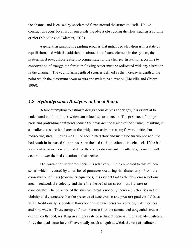
1.2 Hydrodynamic Analysis of Local Scour

Before attempting to estimate design scour depths at bridges, it is essential to

understand the fluid forces which cause local scour to occur. The presence of bridge

piers and protruding abutments reduce the cross-sectional area of the channel, resulting in

a smaller cross-sectional area at the bridge, not only increasing flow velocities but

redirecting streamlines as well. The accelerated flow and increased turbulence near the

bed result in increased shear stresses on the bed at this section of the channel. If the bed

sediment is prone to scour, and if the flow velocities are sufficiently large, erosion will

occur to lower the bed elevation at that section.

The contraction scour mechanism is relatively simple compared to that of local

scour, which is caused by a number of processes occurring simultaneously. From the

conservation of mass (continuity equation), it is evident that as the flow cross-sectional

area is reduced, the velocity and therefore the bed shear stress must increase to

compensate. The presence of the structure creates not only increased velocities in the

vicinity of the structure, but the presence of acceleration and pressure gradient fields as

well. Additionally, secondary flows form to spawn horseshoe vortices, wake vortices,

and bow waves. These complex flows increase both the normal and tangential stresses

exerted on the bed, resulting in a higher rate of sediment removal. For a steady upstream

flow, the local scour hole will eventually reach a depth at which the rate of sediment

4

transport out of the system equals the inflow rate. When this state of equilibrium is

reached, the scour hole depth is known as the local equilibrium scour depth. Figures 1-1

through 1-3 illustrate the flow patterns in the vicinity of a bridge pier.

Pier

VelocityProfile

Bed

Water Level

HorseshoeVortices

Downflow

Figure 1-1 Profile view of a circular pile structure in a steady flow prior to local

scour.

5

VelocityProfile

Pier

Water Level

Bed

HorseshoeVortices

Scour Hole

Surface Roller (Bow Wave)

Downflow

Figure 1-2 Profile view of local scour in a steady flow at a circular pile structure with

local scour.

Flow Separation

HorseshoeVortices

Pier Wake Vortices

Figure 1-3 Plan view of a circular pile structure and the separation of flow, forming a

horseshoe vortex and wake vortices.

Chapter 2 discusses earlier experiments conducted at the University of Florida

and by others to determine how pier design parameters affect local scour.

6

1.3 Need for Research Verification

The discussion above has thus far focused primarily on the scour of non-cohesive

sediments. As the bonding forces in cohesive sediments and rock are significantly

different from those in non-cohesive soils, the forces required to erode these materials are

different. Most sediment scour research to date has focused on non-cohesive sediment

erosion, and as such, the methodologies for estimating design scour depths in rock and

cohesive material have only been developed during the last few years. In the case of rock

scour, in the FHWA Hydraulic Engineering Circular No.18, “Evaluating Scour at

Bridges,” the Federal Highway Administration approached the uncertainty of previous

predictive methods by requiring that all but the hardest of rock be treated as non-cohesive

sediment when computing design scour depths (Richardson and Davis, 2001). That is,

HEC-18 treats all sediment as if it were non-cohesive under the assumption that the bed

materials will erode to the same maximum depths as that of a non-cohesive material,

although the time period required to reach this depth is much longer. This approach

disregards particle bonding and the ability of the material, such as rock or cohesive

sediments, to offer more scour resistance than non-cohesive sediments (Annandale et al.,

1996). This inability to accurately predict design scour depths has cost millions of

dollars in unnecessary construction costs. In response, the Florida Department of

Transportation began sponsoring research programs at the University of Florida with a

primary focus on cohesive sediments and erodable rock. These sediments include clays,

silts, clayey sands, and continuous rock strata which exhibit particle erosion (as opposed

to the removal of rock fragments). Annandale (1996) has developed methods for

estimating scour depths in channel beds composed of hard, fragmented rock. Research

conducted by Sheppard, and others over the past decade have uncovered several

relationships between physical parameters and scour depth that should be accounted for

in bridge design when predicting equilibrium scour depths and calculating pier

embedment in non-cohesive sediments. The results from this more recent research have

been applied to bridge design in Florida by the Florida Department of Transportation.

The University of Florida is a research leader in the field of cohesive sediment

scour. Over the past few years, erosion rate apparatuses have been designed and built

7

and studies conducted for the purpose of measuring the rate at which these sediments

erode as a function of applied shear stress. This information can be used to estimate

contraction and local scour depths over the life of the structure. This research involves

collecting cohesive sediment and rock field samples or creating “manmade” samples,

subjecting them to a range of shear stresses and measuring their rates of erosion. The

information along with predicted flow information at the site can be used to estimate

design scour depths. These apparatus and their use are discussed in Chapters 3 and 4.

1.4 Research Objectives

The University of Florida designed and constructed apparatus capable of

measuring the rate of erosion versus bed shear stress for a wide variety of sediments. The

long-term objective of this research is to obtain a greater understanding of the rates at

which sediments erode and how this property relates to other geotechnical properties.

Due to the complex composition of cohesive sediments and rock a considerable number

of experiments must be performed before these relationships can be established. The

long-term goals of this research include 1) obtaining the ability eliminate the need for rate

of erosion testing for the more scour resistant materials based on the results of standard

geotechnical tests and 2) accurately predicting design scour depths using rate of erosion

test results, and bridge foundation and flow information.

1.4.1 Purpose

The specific objectives of the research described in this report are as follows:

• The continued use of newly developed laboratory apparatus to add to the measured rate of erosion versus applied shear stress database.

• The enhancement and improvement of the hardware and software associated with the rate of erosion apparatus and procedures utilized in reducing and analyzing the data.

• The construction of “manmade” rock and cohesive sediment samples for testing in the erosion rate apparatuses

• The performance of rate of erosion tests with non-cohesive sediments and comparison results with various commonly used total sediment transport formulas.

8

• The development of preliminary models for predicting the relationship between rate of erosion properties and other geotechnical properties.

• The development of models for relating rates of erosion of mixtures of non-cohesive and cohesive sediments to that of non-cohesive sediments.

Chapter 2 of this report provides a brief description of cohesive and rock

materials, presents previous research conducted at the University of Florida pertaining to

local scour in non-cohesive sediments, discusses the current state of knowledge of the

erosive properties of cohesive sediments and rock, and summarizes previously performed

experimental and engineering work. Chapter 3 describes the apparatuses developed at

the University of Florida for measuring rates of erosion, presents recent updates to these

apparatuses, and reviews previous experiments conducted. Chapter 4 describes the

experiments performed as part of this current phase of research work. Chapter 5 presents

the actual data collected from the different experiments listed, and Chapter 6 provides

analysis of the test results, conclusions, and a discussion of future work and

recommendations for improving the erosion rate testing methods and experiments

conducted at the University of Florida.

9

CHAPTER 2 BACKGROUND AND LITERATURE REVIEW

This chapter presents a review of the rock and cohesive sediment erosion process

and discusses research projects that have been conducted in this field. Included are

general descriptions of rock and cohesive sediments, their erosion processes, and current

methods used by practicing engineers to estimate scour of these materials. In addition, a

brief description of the geology of Florida is provided for a general understanding of the

rock and cohesive materials that were evaluated at the University of Florida.

Supplemental resources are also cited in the following sections so that the reader may

better understand the complex nature of Florida’s geology. This is followed by

descriptions of the apparatuses developed and utilized at the University of Florida. At the

end of this chapter an outline of previous rock and cohesive material erosion rate

experiments is given. A discussion of the motivation for the research, the devices used to

conduct the experiments, and the methodology developed to obtain the erosion rates is

presented along with a brief summary of the advantages and limitations of each device

and methodology.

2.1 Rock Description and Scour Behavior

Geotechnical engineering applications require an understanding of the strength

and bearing capacity of rock along with numerous other physical properties. In practice,

rock materials are considered homogeneous and isotropic, although rock is actually

heterogeneous and anisotropic and exhibits a complex and unique particle orientation

specific to the type of rock (Jumikis, 1983). In addition to solid particle composition,

rock samples contain microscopic voids and cracks that result in strength reductions

when subjected to loading tests (Cristescu, 1989). Rocks are classified based on certain

parameters including genesis, geological or lithological classification, and engineering

10

classification based on the strength of intact rock (Henderson 1999; Randazzo and Jones,

1997).

As rock is subjected to high flow rates, a complex erosion process ensues and is

cultivated by a variety of factors. Over time, the forces transferred from the moving fluid

to the rock surface particles weaken the particle bonding between grain particles. Once

the bonds are sufficiently weakened, the particles are separated from the bulk and

transported downstream. The required amount of energy to incite scour in a certain

material of rock or other cohesive sediment is expressed in terms of a critical shear stress

(Henderson, 1999). The skin friction force on a stationary non-cohesive sediment

particle consists of viscous shear stresses that act on the particle surface. Additional drag

and lift forces are produced by differential pressures along the surface of the particle.

With respect to the point of contact, particle movement and separation from the bed will

occur when the moments of the fluid forces are greater than the stabilizing moment from

the submerged particle weight (Van Rijn 1993). Likewise, the particle will move towards

the direction of the least pressure forcing. Further information on the erosion process, the

hydraulic fracturing of rock and alternative rock erosion predictive methods is available

in reports by Henderson (1999), Kerr (2001), and Trammell (2004).

2.2 Approaches to Estimating Rock Scour Prior to Design

• With repeat failures of bridge foundations due to the scour of rock, the FHWA developed a preliminary guide to gauge the susceptibility of rocks to scour by using empirically derived formulas. This preliminary guide, or the “Scourability of Rock Formations” memorandum, is not set up as a permanent set of principles but is instead a document pending the results from research that will improve the ability to evaluate rock for vulnerability to scour (Gordon, 1991). In general, since there is no direct relationships between the scour rates in rock and one single property or condition, engineers should use several different bearing capacity and rock quality calculation methods to find a reasonable idea of scour rates. These methods include subsurface investigation, geologic discontinuities, rock quality designation, unconfined compression strength, the slake durability index, and soundness, and abrasion testing. Further information describing these methods is available in the HEC-18.

11

Before beginning a bridge foundation design in rock, Chapter 2 of the HEC-18

manual states that consultation with local geologists is mandatory in order to understand

what qualities of the base material can impact or limit the design. A geologist or

geotechnical engineer should take rock core samples at the bridge site to determine the

composition of the bed and to perform geotechnical testing. After comparing the

capabilities of the rock along with the expected lifespan of the structure and the expected

hydraulic conditions, a decision can then be made whether the site is appropriate for

construction. A scour competence analysis must first be performed before declaring a

rock material to be susceptible or resistant to scour. Competency depends on the

restrictions set by the “Scourability of Rock Formations” memorandum, geotechnical and

stream stability analysis, hydraulic flume tests, and Erodibility Index testing (Richardson

and Davis, 2001). Geotechnical analysis involves coring the site, performing standard

field classification and soil mechanics tests, followed by mapping the geologic formation

and scour resistance of the immediate environment at the potential structure. Stream

stability analysis requires predictions of changes in flow areas, lateral movement,

directional shifts, etc. due to scour or sediment aggregation (Richardson and Davis,

2001). Annandale’s Erodibility Index quantifies the relative ability of non-uniform earth

material to resist erosion and is defined by multiplying the intact mass strength number,

block size number, inter-particle bond shear strength, and the orientation shape number.

This value is compared with stream power at a pier to determine erosion, where stream

power is defined as the product of the unit weight of water, the unit discharge of water,

and the slope of the energy grade line.

When calculating the pier embedment depth required for the bridge, the HEC-18

states that it is crucial to begin calculating the maximum scour depth according to the

accepted formulas beneath any layers of weathered or erosive rock. The HEC-18 also

stresses the careful removal of any loose or weathered rock layers with minimal blasting

and states that concrete should be poured over the newly exposed area to replace any

removed rock while ensuring maximum contact to prevent water intrusion beneath the

footing (Richardson and Davis, 2001, p. 2.3).

12

2.3 Cohesive Strength of Limestone

In 1992, a study was conducted by McVay, et. al., to investigate rock/shaft

friction values as a response to the increased practice of socketing drilled shafts into

bedrock in order to laterally transmit the enormous loads from foundations. The

experiment involved 14 field-load tests that could be compared with lab experiments to

estimate the socket friction of a shaft in bedrock, and the main question for the

researchers was what magnitude of skin friction was allowable in Florida limestone. The

researchers argued that if the strength in a rock (referring to splitting tensile and

unconfined compression strengths) can be considered a Coulombic material, or having

electrochemical particle interaction, and if the interface skin friction can be used to

approximate the cohesion properties of the rock, then a constant relationship exists

between cohesion and the rock strength. Through numerical analysis, the socket friction

(or “cohesive” strength) can be calculated from the equation below.

tusu qqf21

=

Here, uq represents the unconfined compression strength of a core sample, and

tq represents the splitting tensile strength of a core sample (McVay 1992).

Although the focus of this report is not related to foundation design or drilling

shafts into bedrock, the premise is the same for installing bridge piers into a rock-

bottomed channel. Correlations between rates of erosion and the cohesive strength in

rock will be investigated.

2.4 Cohesive Sediment Description and Scour Behavior

Cohesion occurs as electrochemical, magnetic, or other attractive forces connect

the surfaces of two or more similar bodies. As cohesion is dependent on the ratio of body

surface area to body weight, or the specific surface area, particles with a large surface

area compared to its weight are more likely to develop stronger bonds. A cohesive

sediment is a material in which these inter-particle attractive forces are stronger than the

13

force of gravity drawing them to the bed. Salinity may also play a role in increasing

bonding strength between particles. Cohesion is dependent on mineralogy and water

chemistry qualities, and although particle size and shape greatly impact cohesiveness,

other factors involved require a cohesive sediment to be characterized by its behavior

instead of its size. Cohesive sediments may flocculate in suspension, and once the weight

exceeds the buoyant forces, settling occurs and a mud or fluid mud layer is formed along

the bed. As further particles accumulate and as fluid forces are applied to the bed,

consolidation occurs and the bed material drains and stiffens over a long period of time

(Mehta, 1989).

Difficulties arise when attempting to characterize the behavior of a cohesive

sediment by simply examining individual particle properties. Flocculation of cohesive

sediments is dependent on quantities of organic matter and salinity, where these

additional particles help to provide a base for particles to accumulate and bond together

while in suspension. The flocculated particles are rarely able to maintain a constant

effective particle size as the sediments expand with accumulated sediments and break

apart under hydraulic forces. Because of this variability, the sediment transport

mechanics of cohesive particles are difficult to compare with sand or non-cohesive

sediment scour behavior (Toorman, 2004). With countless parameters influencing the

behavior of fine cohesive sediments, and with the cost inefficiency in testing each of

these qualities, only the properties and conditions that primarily affect scour resistance

should be focused on. These properties include organic and inorganic material content,

mineral composition, gradation, flocculation size and orientation, strength, permeability,

and water temperature, salinity, pH and ion concentrations. The concentration of ions in

water along with the presence of non-sediment compounds interacting with the

suspended sediments greatly impact the corresponding resistive force to bed shear

stresses induced by water flow, while acidic pH levels tend to aid the sediment ability to

flocculate (Mehta, 1989). Another important property for a cohesive sediment’s ability to

flocculate is the cation exchange capacity. As the cation exchange capacity increases, the

ability of particles to cohesively bond to other particles increases, and flocculation results

as the effective particle diameter increases. Also, as voids are trapped between particles

14

during the bonding process and allowed to settle, the particles may be able to erode more

rapidly than if the mixture was completely solid.

Scour may be observed in cohesive sediments through aggregate-by-aggregate

surface erosion, mass erosion of a bed, or re-entrainment of suspension. Aggregate-by-

aggregate erosion occurs as flocculated particles are removed individually from the

channel bed and is typically observed under minimal flows around the sediment critical

shear stress. The mass erosion of a bed is typical for higher fluid velocities and much

higher bed shear stresses than the sediment shear resistance, where relatively large pieces

of sediment are pulled from the bed and removed from the system. Sediment re-

entrainment is caused by variations in the bed shear stress and fluid velocities, which can

cause the flocculated particles to cycle between suspension and settling.

As expected, the best way to determine the bed critical shear stress and erosion

rates for a cohesive sediment is through the use of physical models and flume studies that

measure scour rates directly. While some uncertainty in testing samples exists due to

inflicted disturbances to the sample during collection, and although the water utilized for

experimentation does not match the makeup of the water at the actual bridge site,

valuable predictions can still be obtained for cohesive sediment scour through normal

flume testing (Mehta 1989).

2.5 Methodologies to Estimate Cohesive Sediment Scour Prior to Design

According to the HEC-18, time for maximum scour to occur is the only

differentiating factor in design for cohesive sediments and non-cohesive sediments. The

data on which this assumption is made is, however, extremely limited. If a bridge is

constructed on scour resistant cohesive bed, and the design life of the bridge is short in

comparison to the expected number of scouring floods, scour depth estimates may be too

conservative. Substantial cost savings can be achieved through the use of alternative

scour prediction methods under these conditions and a cohesive bed environment

(Richardson and Davis, 2001).

15

In cohesive sediment beds, it is important to factor in the time rate of scour when

calculating scour depth. In non-cohesive soils, one major flood event may allow for

absolute equilibrium to be reached, where the maximum scour depth is achieved and no

further scour can occur. However, in cohesive sediments, the maximum scour depth is

dependent on many years of flood history, and the amount of scour experienced in a

similar flood event could only be a small fraction of the depth achieved in the non-

cohesive sediment scour example. Thus, knowing the time rate of scour in relation to a

given shear stress is crucial, as this relationship can then be used to calculate the

maximum scour depth of the cohesive sediment (Richardson and Davis, 2001).

One method of calculating erosion rates is through the Scour Rate in Cohesive

Soils (SRICOS) method. This method requires the collection and laboratory testing of

several sub-surface cored samples taken from a site of interest. The method calculates

the applied shear stress on a sample as

τmax = 0.0094ρ⋅ V2 1log Re( )

110

−⎛⎜⎝

⎞⎟⎠

⋅,

where ρ is the density of water, V is the mean approach velocity, and Re is the pier

Reynolds number. The initial scour rate corresponding to τmax is then read from the rate

of erosion vs. shear stress curve and the maximum scour depth, zmax is calculated using

the HEC-18 pier scour equations. The total amount of scour can be predicted by applying

a history of shear stress values over the design life of the bridge and finding the

subsequent periodic scour assuming no aggregation or sedimentation. This method is

limited to circular bridge piers and for water depth to pier ratios greater than 2, but

correction factors can be applied for some alternative cases (Richardson and Davis,

2001).

16

2.6 Local Scour Research in Non-Cohesive Sediments

One objective of the current research is to discuss comparisons between erosion

rate-shear stress relationships for cohesive and non-cohesive sediments. Additionally, as

the experiments of this report do not directly focus on local scour experimentation. The

erosion rate results from the apparatuses at the University of Florida can, however, be

used to estimate design contraction and local scour depths. Before addressing this further,

it is important to present pier scour studies and laboratory experiments conducted in non-

cohesive beds.

In 1988, Bruce Melville at the University of Auckland presented a design method

for local pier scour which allowed the designer to follow flow charts in order to calculate

the limiting armor velocity (the minimum velocity at which armoring of a non-uniform

channel bed is impossible) and the local scour depth. According to Melville, the

maximum scour depth that will occur in non-cohesive sediment beds is equal to 2.4 times

the pier diameter, but that under certain conditions, the scour depth can be reduced. It

was noted that in shallow depths, the surface roller or bow wave can interfere with the

scouring action of the horseshoe vortices since the two have opposite rotation. For

shallow water depths, larger sediment grain sizes, and clear water scour conditions,

Melville argued that pier scour depths could be reduced with the reduction of the 2.4

multiplying factor. Melville presented the local scour depth as a function of

dimensionless flow intensity (V/Vc), the ratio of flow depth to the pier diameter (y0 /D),

the ratio of pier diameter to sediment grain size (D/D50 or b/D50), and shape and

alignment factors. Data was compiled relating these parameters and others to

dimensionless scour depth parameters in order to develop a design method for bridges

(Melville and Sutherland, 1988).

More recently, Sheppard at the University of Florida conducted a number of

clear-water and live-bed local scour experiments in several laboratories in the U.S and in

New Zealand. Based on his data and that of a number of other researchers he developed a

normalized local equilibrium scour depth equation that depends on three quantities,

0yD *⎛ ⎞⎜ ⎟⎝ ⎠

, c

VV

⎛ ⎞⎜ ⎟⎝ ⎠

, and 50

D *D⎛ ⎞⎜ ⎟⎝ ⎠

. The equation has the following form:

17

⎟⎟⎠

⎞⎜⎜⎝

⎛⎟⎟⎠

⎞⎜⎜⎝

⎛⎟⎠⎞

⎜⎝⎛=

5032

01

**

5.2* D

DfVVf

Dy

fDd

c

se ,

where dse is the equilibrium scour depth, and D* is the effective pier diameter,

which is equal to the actual diameter for circular piers, y0 is the water depth, V the depth

averaged velocity, Vc the sediment critical velocity and D50 the median sediment diameter

(Sheppard, Odeh, and Glasser 2004).

The equations for clear-water and live-bed conditions are given below:

Clear-water scour range (0.47≤ V/Vc ≤ 1):

⎪⎭

⎪⎬⎫

⎪⎩

⎪⎨⎧

⎥⎦

⎤⎢⎣

⎡⎟⎟⎠

⎞⎜⎜⎝

⎛−⎟⎟

⎠

⎞⎜⎜⎝

⎛⎟⎠⎞

⎜⎝⎛=

2

502

01 ln75.11*

*5.2

* c

se

VV

DDf

Dy

fDd

Live-bed scour range up to the live-bed peak (1≤ V/Vc ≤ Vlp/Vc):

⎥⎥⎦

⎤

⎢⎢⎣

⎡⎟⎟⎠

⎞⎜⎜⎝

⎛

−

−⎟⎟⎠

⎞⎜⎜⎝

⎛+⎟

⎟⎠

⎞⎜⎜⎝

⎛

−−

⎟⎠⎞

⎜⎝⎛=

1///*5.2

1/1/

2.2** 50

20

1clp

cclp

clp

cse

VVVVVV

DDf

VVVV

Dy

fDd

Live-bed scour range above the live-bed peak (V/Vc > Vlp/Vc):

⎟⎠⎞

⎜⎝⎛=

*2.2

*0

1 Dy

fDd se

where

⎥⎥⎦

⎤

⎢⎢⎣

⎡⎟⎠⎞

⎜⎝⎛=⎟

⎠⎞

⎜⎝⎛

4.000

1 *tanh

* Dy

Dy

f

and

( ) ( ) 13.050

2.150

50

502 /*6.10/*4.0

/**−+

=⎟⎟⎠

⎞⎜⎜⎝

⎛

DDDDDD

DDf

A possible explanation for the scour depth dependence on 50

D *D

is given in

Sheppard (2004), ascribing this D*/D50 dependence to the pressure gradient field in the

vicinity of the structure created by the structure.

18

2.7 Previous Flume Studies of Rock and Cohesive Sediment Scour

In addition to the flume developed at the University of Florida, which will be

discussed in Chapter 3, several researchers have developed laboratory flumes in order to

test scour rates in cohesive soils. These include the Erosion Function Apparatus (EFA),

the Sediment Erosion at Depth Flume (SEDFlume), and the Adjustable Shear Stress

Erosion and Transport Flume (ASSET).

2.7.1 Erosion Function Apparatus (EFA)

The EFA was developed by Briaud et al. for measuring the scour rate in cohesive

sediments and is used to calculate rate of scour and maximum scour depths. The EFA is

a rectangular flume, 101.6 mm x 50.8 mm in cross section and 1.22 m allowing for 0.1 to

6.0 m/sec flow velocities. A Shelby tube containing a sediment sample may be inserted

through bottom of the flume to expose the sample surface to flow (Briaud, 1999). For

testing in the flume, once the sample is inserted and allowed to saturate in the flume, the

velocity is initially set to 0.3 m/s. The sample is projected 1 mm into the channel, and the

time to erode this 1 mm length of sample indicates the rate at which scour occurs. The

test is repeated for a full range of increasing flow velocities, maximum shear stresses are

calculated, and the SRICOS method and chapter 6 of the HEC-18 is used to determine a

maximum scour depth (Briaud, 1999).

With the setup of the EFA, in addition to bed shear stresses, normal

stresses are introduced to the sample with a protruded length. Stronger forcing would

result in higher erosion rate observed for the given flow velocity, leading to a more

conservative relationship between shear stress and rate of scour. Also, calculating the

shear stress in terms of flow velocity may not be appropriate due to accuracy issues

concerning the paddle-wheel flow meters, leading to an incorrect estimation of the shear

stress. The 1 mm protrusion length can be difficult to measure visually. The EFA is

heavily dependent on operator judgment for advancing the sample, which reduces

experiment repeatability and increases opportunity for human error. The EFA has been

useful, however, in providing foundational relationships between shear stress and the

19

erosion rates of rock and cohesive sediments; the results from these experiments have

been employed in bridge construction to save construction and material costs.

2.7.2 Sediment Erosion at Depth Flume (SEDflume)

The SEDflume was developed by Wilbert Lick at the University of Santa Barbara

and was designed to track the transport and suspension rate of contaminants with fine-

grained sediments during large flood events. The flume is designed as a rectangular

flume 2 cm in height, 10 cm in width, and 120 cm in length, and water is pumped into the

flume and through a 10 cm wide, 15 cm long, and 1 m deep test section. A portable field

unit version of the SEDFlume has since been in design and implementation. To test a

sample in the flume, a coring test container is filled with either reconstructed or

undisturbed sediments and inserted through the bottom of the test section. An operator

manually advances the sample using a piston with a variable speed screw-jack motor to a

point where sample surface is flush with the flume bed. The flume is filled with water,

and when a constant flow is reached, the shear stress exerted results in sediment erosion.

As the test continues, the operator uses visual inspection to continuously advance the

sample, maintaining a level sediment-water interface with the channel bed surface. The

shear stress on the bed surface is calculated based on the average flow velocity, and the

rate of erosion observed is equal to the amount of sediment advanced over the experiment

duration at a specific flow velocity (McNeil et al., 1996).

2.7.3 Adjustable Shear Stress Erosion and Transport Flume (ASSET)

As an updated and larger version of the SEDflume, the ASSET Flume is used to

directly measure erosion rates as a function of applied shear stress while quantifying the

sediment transport in terms of depth. In order to minimize the effects of the flume wall

on the development of flow and its subsequent response to the sample surface, the

ASSET Flume was constructed larger than the SEDFlume. Three bedload traps with

baffles were included to collect and quantify the amount of sediment transported due to

shear stress. Samples are advanced using a manual screw-jack to where the sample

surface is flush with the bed of the flume, where visual inspection is required to set the

20

surface elevation. Unlike the SEDFlume, the sediment collected in the bedload traps

must be oven-dried and weighed to calculate the bedload fraction and the suspended load

fraction. These factors are used to calculate the rate of erosion based on the ability of the

hydraulic conditions to transport sediment away from the test section (Roberts et al.,

2003).

The ASSET Flume and SEDFlume share the same disadvantages of the EFA in

that the calculation of shear stress is dependent on the channel mean velocity, and the

paddle-wheel flow meters may provide inaccurate velocity readings, leading to an

incorrect shear stress measurement. Also, as the distance a sample is advanced is based

on visual inspection, it may be difficult to determine when the sample elevation is flush

with the flume bed. Because of the transition of the bed roughness from smooth metal to

rough grains of weaker resistance, uneven erosion may be evident which create operator

difficulties when trying to determine a mean elevation. Thus, repeatability of

experimentation would be difficult to achieve, and this creates concerns if there is a

limited number of samples available for testing.

On the other hand, the SEDFlume allows for direct correlation of applied shear

stress and indirect correlations of bulk density, water content, and organic particle size

and content to erosion rates and critical shear stress as functions of depth. Another very

useful aspect of the portable SEDFlume is that the water from the site of implementation

can be used directly, and so the results of testing are more meaningful and realistic to the

unique conditions of the area. By using water from the site of interest, it may be more

difficult to obtain generalized solutions without first knowing the chemistry and physical

properties of the water, and another concern would be inconsistencies in water quality

and unknown sediment suspension concentrations. In any case, the results from testing in

the field would give different results than what would be seen for clear water scour

testing from laboratory studies.

2.8 Scour in Sediment Mixtures

Procuring field samples can be a costly ordeal, and ensuring that the samples

reach a laboratory flume device without disturbing the integrity of the core can be

21

difficult. Also, since testing specimens for rates of scour requires the destruction of the

core, multitude samples are needed in order to confidently establish an accurate

relationship between applied shear stresses and erosion rates. For flume studies that

examine a larger section of a channel bed for pier scour, obviously an actual channel bed

cannot be transplanted into a laboratory flume. Historically, most pier scour flume

studies have been conducted using beds composed of non-cohesive sands of different

gradations. Realistically, however, most channel beds are composed of non-

homogeneous sediment mixtures, and rarely could one find a bridge site consisting of

pure sands or non-cohesive soils. Since the HEC-18 sets the procedure for evaluating

scour depths in cohesive sediment environments as the same for sand (except for an

extended duration for maximum scour to occur), and since testing cohesive sediments

requires controlling several additional experimental variables, the problem of measuring

scour rates in cohesive mixtures historically has not been a priority for many researchers.

From 1991 to 1996, experiments were designed and conducted to tackle the

problem of estimating scour depths at bridge piers and abutments in channels with

cohesive and non-cohesive sediments at Colorado State University. The primary focus of

this study was to test the effects of sediment gradation and cohesion on scour

development, and experimentation involved testing 20 non-cohesive sediments and 10

cohesive sediment mixtures in five different flumes of various sizes with nine different

cylindrical pier sizes and seven different abutment protrusion lengths. The overall

experiment was grouped into four sections which involved the study of the effects of

gradation and coarse bed material fraction on pier scour, the effects of grain size fraction

on abutment scour, the effects of bed clay content on pier scour, and the effects of

cohesion on pier scour with a bed composed completely of clay (Molinas 2003).

Of particular interest to this research is the study involving heterogeneous channel

beds with cohesive sands, or sands mixed with clay. For several different scenarios of

various clay/sand ratios, flume types, and flow conditions, pier scour was observed and

visually measured in terms of the flow velocity. Three flumes were utilized in this

experiment: a river mechanics flume (5 m x 30 m), a sediment transport flume (2.4 m x

60 m), and a steep flume (1.2 m x 12 m). To maintain the integrity of the experiment,

only the flow velocity and clay content were permitted to vary, while the circular pier

22

maintained a diameter of 0.15 m, and the approach depth was equal to 0.24 m. The

sediments used in the study were Montmorillonite clay and sand with a median diameter

of 0.55 mm with a gradation coefficient of 2.43. Clay contents were allowed to vary

from 0 to 11 percent, and the scour observed was compared to that observed in beds

exclusively composed of sand. The procedure for conducting scour tests is similar to

other scour experiments; flow is initiated by specifying a low frequency pump speed, and

the pump speed is slowly increased until the desired flow velocity is reached.

According to the results of the experiment, as the percent of clay content

increased, the maximum scour depth decreased. An expression that best matches the data

was given as:

9.0

111

1

⎟⎠⎞

⎜⎝⎛+

=CC

KCC ; 110 ≤≤ CC

CC represents the percent clay content in the sediment mixture, and CCK is a

scour reduction factor comparing the scour depth observed in pure sand and the scour

depth observed in the clayey sand. CCK ranges from 0 to 1, where 1 equals the scour rate

observed in sand under the same flow conditions. Scour depths for clay contents higher

than 11 percent were shown to be dominated by the initial water content and

consolidation, and since these factors were not controlled in the experiment, data for

these samples was not included when determining a formula.

While this study has exhibited a very thorough approach to examining the scour at

bridge structures in cohesive material, and although the authors expressed that the

formulas produced were not intended for general application, there are a few problems in

the design of this experiment that could negatively affect the formula produced. The

issue of most concern is the gradation range used in every experiment. The grain size

standard deviation for sand, gσ , was maintained at 2.43, which is probably too large of a

spread for accurate testing. The grain size standard deviation was calculated using the

following equation.

23

⎟⎟⎠

⎞⎜⎜⎝

⎛+=

16

50

50

84

21

DD

DD

gσ .

Larger sand grain particles naturally require larger forces to initiate transport than

smaller particles. At slower pump speeds, the fine grains near the surface are transported

away while larger grains are left in place. As larger grains settle in to fill the voids

created by the escaping finer grains, a scour resistant armor layer is developed that

protects deeper fine sediments from erosion. If velocities increase in the channel, the

armor layer will scour away which will expose the fine particles underneath, resulting in

a high rate of erosion. As there is a reduction in scour depth as the clay content

percentage increases, with a large spread over the range of grain sizes, there is question

of whether the scour resistance observed is due to cohesion alone or due to the armoring

effect of the largest sand particles. Surely, the strengthening of the bed is due to a

combination of these two properties. To provide a more meaningful analysis of the

impact of clay content on bridge scour, it would be more practical to use a uniform grain

size to eliminate the occurrence of armoring. This observation will play a role in the

design of sediment samples tested in the erosion measurement apparatuses at the

University of Florida.

Another issue of concern involves the use of recirculating sediment flumes. The

sedimentation flume (used in both the clayey sand study and the exclusively sand study)

and the hydrodynamics flume (used in the sand experiment) allow sediment to erode

from the study area and remain in the flow. The introduction of sediments to the

approach flow change the clear water scour condition to a live bed scour condition, which

would compromise the experiment. The duration of time required for the formation of a

scour hole is longer in cohesive sediments, and even as the experiment could be halted at

the first sign of sediment recirculation, there can be no assurance that the scour hole has

been allowed to develop to completion.

In a University of Florida thesis investigating the effect of suspended fine

sediment on the development of local scour depths, a similar experiment involving pier

scour was set up in a natural channel and observed for several days. Storm events during

testing would loosen upstream sediment and change the suspended sediment

24

concentration in the approach flow to the pier. During and after these storm events, the

scour hole in development would halt formation until the flow conditions returned to

normal. It was observed that fine sediments entrained in the flow may dampen the

turbulence and reduce the Reynolds stresses and consequent bed shear stresses. Thus, it

is crucial to avoid the introduction of suspended sediment into the upstream water supply

as the scour hole may not develop to completion as it would under clear water conditions.

25

CHAPTER 3 REVIEW AND UPDATE TO THE EROSION RATE LABORATORY APPARATUSES

This chapter discusses the laboratory apparatuses constructed at the University of

Florida for measuring the rates of erosion in rocks, cohesive sediments, and non-cohesive

sediments. The two apparatuses are known as the Rotating Erosion Rate Test Apparatus

(RETA) and the Sediment Erosion Rate Flume (SERF). Five RETA units have been

constructed and are maintained and operated at the FDOT State Materials Laboratory in

Gainesville, Florida, while one SERF unit is available and located at the University of

Florida. Both the RETA and the SERF units are unique in that they measure the rate of

erosion of a specimen with regard to the shear stress exerted instead of the flow velocity.

3.1 Rotating Erosion Testing Apparatus (RETA)

3.1.1 Description

In order to estimate the rate at which sediment erodes due to shear stress applied

by the flowing water, the Rotating Erosion Test Apparatus (RETA) was developed. As

the RETA is not a flume-based apparatus, its function is to provide erosion rate as a

function of applied shear stress information for sediments with sufficient bonding

strength to support their weight. Sediments that qualify for testing in the RETA include

stiff clays, sandstone, limestone, coquina, and any other rock or self-supporting material.

The RETA is designed to house a cylindrical specimen, and a rotating outer cylinder

initiates the flow of water around the full longitudinal surface of the sample. The shear

stress exerted on the sample from the flow is designated for each test, and the rate of

erosion is based on a loss of mass and is calculated for a range of shear stress values.

Considering the slow rate at which rock may scour, the apparatus is capable of testing

samples at very high shear stresses for extended durations on the order of several days.

26

Five RETA units have been made available for use with the intent of testing several

similar specimens simultaneously so that the repeatability of testing may be confirmed

(Kerr, 2001).

The RETA is available in two sizes for testing either a 2.4 inch or 4 inch diameter

cylindrical specimen of 4 inches length. For securing a sample into the RETA and to

provide a connection between the bottom and top plates which cap the ends of the core, a

¼ inch diameter hole is drilled through the longitudinal central axis of the sample for the

insertion of a support shaft. The upper end of the support shaft connects to a torque-

measuring load cell with a slip clutch, while the lower end of the shaft is connected to the

motor. A motor control system allows the user to specify the torque to exert on the outer

rotating cylinder. The outer cylinder, which is connected to an electric motor by pulleys

and a belt, is rotated in order to create a shear stress on the surface of the sample. The

shear stress increases with increasing angular speed of the outer cylinder.

The torque cell is comprised of a moment arm attached to the support shaft the

end of which rests against a load cell. Two mechanical stops are used to apply a slight

pre-torque to the load cell and to prevent the applied torque from exceeding the limiting

force on the load cell. An adjustable torque clutch is located between the sample and the

torque cell. The purpose of the clutch is to prevent damage to the system in the event that

a fragment of the sample separates and lodges in the annulus between the specimen and

the outer cylinder. The slip torque is set at slightly higher than the maximum anticipated

torque value under normal operation. If the torque exceeds the maximum anticipated

value, the clutch will slip, and the control system turns off the outer cylinder drive motor.

Earlier versions of the RETA used a torque cell instead of a load cell in order to measure

the torque on the sample. In addition to the torque cell, a spring was used in the unit that

would slightly turn with increasing torque, and this extension of the spring would be

registered by the torque cell. The RETA was redesigned to remove these components

due to the tendency of the torque cells to malfunction or break during testing, while

working with a spring constant was not preferred as it may give unreliable results and

change over the lifespan of the unit. The updated RETA, which employs the moment

arm and load cell, is a design which reduces the complexity and size of the torque

27

measurement unit. Drawings for the components of the RETA system are given in

Appendix A.

A control system was developed for the RETA that allows either the torque or a

rotational speed to be specified. When the torque is specified, the control system

increases the rotational speed of the outer cylinder until the torque applied to the sample

reaches the target level. It then maintains this torque until the unit is either stopped or the

desired torque is changed. In this mode, if there is a change in anything that would

impact the torque (such as a water temperature rise) the rotating speed will be adjusted so

as to maintain the prescribed shear stress. In the rotating speed mode, the rotating speed

is simply held at the desired constant value.

Since tests can run for more than 24 hours at a time, friction develops due to the

rapid flow of water through the annulus, resulting in an increase in temperature. The

friction creates a significant amount of heat which previously resulted in some

evaporation, and consequentially there was a change in the shear stress exerted on the

sample. To compensate for this, a water cooling system has been added to provide a cool

water drip to the system, replacing the evaporated water and better controlling the water

temperature.

3.1.2 Testing

Some sample preparation is required before testing in the RETA. This may

require shortening the sample or turning down the sample in a lathe in order to smooth

down the outer edge. After drilling the hole through the central axis and installing the

support shaft and end plates, the oven-dried mass of the sample is recorded, and the

sample is allowed to saturate inside the RETA unit. To do this, the sample is placed

inside the RETA cylinder, connecting the support shaft to the load cell and the motor, and

the annulus is filled with water. First, a small torque is set to initiate a gentle spin that

will remove any loose or weakened particles on the sample edges. It is important to

allow this initial spin to last at least 12 hours to ensure that all loose particles are

removed, or otherwise the first RETA test will indicate an abnormally higher rate of

erosion. The sample is then removed from the unit, the water is drained, and the outer

28

cylinder and sample are gently rinsed. As the RETA calculates rates of erosion based on

the mass lost from a specimen, the physical properties of the specimen must first be

gauged before testing commences. In addition to the dry mass, sample dimensions and

saturated mass of the sample are recorded in order to calculate surface area, density, and

volume (Kerr, 2001).

To begin testing, the specimen is placed into the slightly larger RETA cylinder

with a sleeve insert, the annulus is refilled with water, and the lowest desired torque or

rotational speed is set. The duration of testing depends on the scour resistance of the

sample, and can be determined as the operator visually observes the rate of erosion. For a

rock core, each test may require a minimum of 72 hours. After testing, the sleeve with

the water and eroded sediment is placed in an oven and the water is evaporated. The

dried sediment and sleeve are weighed, and the combined weight subtracted from the

known weight of the sleeve to determine the mass of eroded material. The average shear

stress is calculated using the formula:

2

T Average Shear Stress = 2 R L

τ ≡π

,

where T represents the specified torque measured by the load cell, R represents

the radius of the core, and L is the length of the sample. The rate of erosion is calculated

as

r mt RLD

,Δ Δ=

Δ πρ2

where Δr is the average change in radius of the sample during the test (calculated

from the eroded mass), Δt and D represent the duration of the test, Δm represents the

mass removed from the specimen during testing, and ρ equals the dry mass density of the

sample. When conducting erosion rate tests in the RETA, a minimum of three (and

preferably five) tests should be performed. With more data points from testing similar

samples at the same location, a relationship between erosion rate and shear stress may be

determined.

Examples of the advantages of the RETA include 1) it provides a direct

measurement of torque (shear stress), 2) higher shear stress levels can be obtained, and 3)

29

long duration tests do not present problems. Disadvantage of the RETA include 1) the

shear stress is exerted along the vertical plane of the sample (instead of the horizontal

plane as in nature), 2) the ability to test only self-supporting samples, and 3) the effort

and time required to measure the eroded material.

3.2 Sediment Erosion Rate Flume (SERF)

3.2.1 Equipment Description and Developments

The second and most recent rate or erosion apparatus designed and constructed at

the University of Florida, the Sediment Erosion Rate Flume (SERF), is capable of

directly measuring sediment erosion rates while subjected a water flow-induced shear

stress. The shear stress is, however, obtained indirectly from measurements of pressure

drop in the flume. The computed shear stress is thus the average shear stress on the four

sides of the flume over the distance between the pressure taps.

The test area of the SERF is a flume with a rectangular cross-section. The SERF

system consists of the flume, an 1100 gallon reservoir, two parallel pumps and the

connecting plumbing. The flume is mounted on 5.5 ft high supports. Water is supplied to

the flume from an 1100 gallon reservoir. The reservoir is equipped with a series of

baffles to reduce the amount of turbulence in the tank and aid in the settling out of any

suspended sediment. The tank is also equipped with a 2 ft port on the top and a drain

valve for ease of cleaning between tests. The piping between the tank and the two pumps

is 6 inch schedule 80 CPVC, and the piping between the pumps to the flume is 4 inch

schedule. 80 CPVC.

Flexible couplings are located at the discharges of the two 500 gpm pumps in an

effort to mechanically isolate the pumps from the flume. There are shut off valves at the

discharges of the reservoir and pumps to provide increased flow control and prevent any

backflow of water into the pumps. Water discharged through the pumps is carried

through the 4 inch pipe to the circular to rectangular transition section.

As water enters the flume, it first passes through a 1 ft long flow straightener.

This reduces the scale of turbulence or vortices which may be present in the flow and aids

30

in the transition to a hydraulically smooth, fully developed flow. The flow passes

through a 3 ft length of flume before reaching the 1 ft test section. The flow then passes

over the sediment sample centered in the bottom of the test section, then through 4

additional feet of flume before reaching the rectangle to circular transition to the flexible

pipe to the reservoir.

The test sample housing is mounted to the bottom of the test section. The test

housing consists of an acrylic cylinder secured by two compression plates. The top plate

is mounted to the bottom of the test section of the flume, while the bottom plate is

attached to the top plate through four bolts which support and secure the cylinder in a

compressive manner, permitting sample removal without disassembling the entire test

section. In addition, the top of the test section is equipped with a port through which the

SeaTek ultrasonic transducer is mounted. Located on the side of the test section is a 1.4

inch diameter window through which a camera is able to display a real-time image of the

sample eroding via a closed circuit television system. The stepper motor is bolted to a

variable elevation stand mounted to the floor underneath the test section and is easily

positioned directly under the test cylinder. The sample is driven up by the motorized lead

screw and plunger inside of the test cylinder. Refer to Trammell, 2004 for review of the

schematic drawings of the flume and components.

While the experiment is underway, a camera positioned at the test section window

displays the erosion process as it progresses. This is viewed via a television in the

control office, which also records the video image to a high-8 video recorder. Although

the program is capable of running continuously without input from the user, there is still

need for human control to ensure proper testing. In particular, if large chunks of

sediment break off from the sample, and the sample consequentially protrudes into the

flow, the test should be stopped and restarted. Also, the ability to have each test backed

up on video is a very useful advantage. This allows for future researchers or designers to

see exactly how a certain material will erode under the specified conditions.

The two pumps used for the erosion rate and critical shear stress testing are each

controlled separately by the lab technician running the test. If a “soft” sample, such as a

soft clay or sand, is being tested, the use of only one pump is required and the variable

31

frequency drive pump is used. This pump is controlled using a keypad in the control

room, and its speed is increased by slowly increasing its frequency. The full range of the

frequency drive pump is 60 Hz, and the incremental steps may be set as low as 0.01 Hz.

For “hard” samples such as rock or stiff clay, both pumps may be used. First the variable

speed pump is slowly brought up to full speed. Once it begins operating at 60 Hz, the

variable speed motor is shut down and the on/off pump is started. The variable speed

motor is then slowly stepped up until the desired velocity and shear stress is achieved.

The differential pressure measurement system has been significantly updated over

the past year. Originally, one Sensotec pressure transducer bracketed to the motor stand

was connected by clear plastic tubing to two pressure ports located on the underside of

the flume. These pressure ports are positioned 2 ft from the center of the test section and

connected to the transducer through the use of brass compression fittings and clear plastic

tubing. As the differential pressure was measured over 4 ft for a 2.3 inch sample,

questions arose over whether the pressure drop observed was due to the sample and not

the flume walls. Also, because the connective tubing was connected to the underside of

the flume, when testing with small shear stresses, sediments would erode and

subsequently clog the downstream pressure port. This will naturally result in erroneous

shear stress reading. To compensate for these concerns, two new sets of pressure ports

were installed into the side walls of the flume. Currently, there are additional sets spaced

2 feet from the test section and 2 inches from the test section, each located on the side

wall at half the channel height. The set of pressure ports spaced 4 inches apart is

connected to a more sensitive transducer capable of reading much smaller differences in

shear stress. This specific transducer has the ability to measure a maximum pressure

difference of ten inches of water. With this transducer, the pressure drop observed

directly across the sample can be measured, and these readings can be compared with

pressure readings from the longer spanned pressure ports. The pressure taps were

installed on the side wall of the flume opposite of the camera instead of from the bottom

of the flume so as to not come into contact or interfere with the specimen itself.

Positioning the pressure taps from the side wall is advantageous in that it does not allow

eroded sediment particles to fill the plastic tubing which lead to the pressure transducer

and return faulty pressure readings. In the past, most SERF testing required the pressure

32

tap lines to be flushed periodically in order to remove any sediment build up or clogging,

and this often limited the duration for testing, especially when testing finer sands and

clays. The set of pressure ports spaced 4 ft apart is currently connected by tubing to a

manometer. In order to read the differential pressure under heavy pump flows,

compressed air should be pumped into the air space separating the two water columns.

The difference in water height is measured directly from the manometer in order to

calculate the pressure difference. These other pressure monitoring systems allow the

operator to compare shear stress readings and improve precision in testing.

Previously in the SERF, it was observed that some clays are guilty of absorbing or

scattering some of the signal sent by the SeaTek. Since the signal was penetrating deeper

into the sample, the SeaTek returned faulty, inconsistent data and either protruded the

sample into the channel or caused the sample to oscillate. This is problematic since

sample protrusion into the flow introduces normal stresses that can contribute more

strongly to scour than direct bed shear stresses. Several measures have been taken that

would increase signal strength and reduce outside noise. The primary change was

attaching the SeaTek’s power unit and electrical system to the downstream flume support

instead of being housed in an adjacent office. By reducing cable length, the system

would be less affected by electrical noise in the area.

Replaced components of the SERF include a new stepper motor unit and a new

primary differential pressure transducer. As the stepper motor is set beneath an opening

in the flume through which the sample is advanced, exchanging a sample or taking the

apparatus apart usually results in some water drainage from the flume. Over time, as the

stepper motor gradually became further exposed to water, the motor lost functionality and

resisted or limited signals from the computer to advance the specimen. The stepper

motor was replaced and supplemented with a clear plastic sheet to shield the unit from

water exposure. The shield attaches to the top of the lead screw and is pinned into the

plunger along with the lead screw, and the cover drapes down the sides of the motor to

guide all water away from the system. New inline valves were installed in the pressure

tube lines, as well as a camera mounting bar attached to the flume supports in order to

keep the camera in place and resistant to vibration from the flume. To prevent the

stepper motor from advancing a sample too far or too low (where water may exit the

33

flume through the test section), a housing for limit switches was installed. If desired,

limit switches may be added which will turn off the stepper motor in the event of an out-

of-range descending or ascending signal from the LabVIEW program. The housing unit

consists of two threaded rods extending beneath the stepper motor mount, and as the

motor lead screw passes either a high or low specified elevation, the switch will be

activated and abort the test before the system is damaged or the lab environment is

flooded.

3.2.2 Computerized Control Description and Updates

In order to minimize operator input and reduce subsequent human error factors,

the SERF is managed through LabView software on a computer control station. Using

the SeaTek ultrasonic transducer, elevations of the sample and of the test section bed are

determined. Of the twelve transducers contained within the SeaTek, four measure the

outside bed elevation, and eight measure the inner bed elevation. The control station

houses the computer unit running the software, the control system for the SeaTek unit, a

closed-circuit television for visual monitoring, and a pump frequency control system

(Trammell, 2004).

The output data from the SeaTek control is typically averaged over twenty sample

readings (user defined). That is, the output value for a particular channel is the average

of twenty return signals for that channel. These distances are inputted into a LabView

program, and an average of the sample surface elevation is calculated and compared

against an average of the flume bed surface elevation. If the difference is greater than 0.5

mm, the program signals the stepper motor to move the sample to where it is flush with

the bed. Once completed, a new set of numbers is retrieved from the SeaTek and the

process repeats. If the stepper motor oversteps the desired amount, (due to erroneous

SeaTek data or particle stacking), the LabView program will step the sample down to

where it is flush with the bed. For samples expected to erode in large pieces or behave

irregularly, the program averages the sample elevations excluding the highest and lowest

values. In addition, signals from potentially faulty transducers can be easily removed

from the data set.

34

Once the program obtains the elevations and moves the motor (if required), the

program records the shear stress, elapsed time, distance stepped, average pressure, and

average temperature to a text file. The pressure and temperature are recorded using a

data acquisition PCI card and a signal conditioning terminal block. The signal

conditioning reduces the amount of noise in the signal and allows for a more accurate

average. The data from these two instruments is constantly streaming; however, when a

data file is written it takes 100-500 readings (user specified), determines the mean of

these readings, and then records this value into the data file. If motion is not initiated

within a user defined time increment, a data file is written recording the same parameters

from above, allowing the user to review data to ensure that all of the measurements

recorded remain constant.

The SERF computer operating system has recently been upgraded to focus on

and improved averaging techniques used to determine the average depth of the sample in

the channel. Previously in the LabVIEW program, the SeaTek would send a string of

data to the computer, consisting of a date, time, the values of the eight inner transducers,

and the value of the four outer transducers. From the string, the first section was

removed in order to separate the date and time from actual data, and a search was done in

the string for any values that equaled zero (indicating an invalid reading from the

SeaTek). All zeroes were removed from the string using a while loop. The remaining

values were then organized into an array and averaged, and the difference in average

between the inner and outer transducers determined the distance required by the stepper

motor to advance, achieving a level bed surface. However, it was observed that the

SeaTek frequently sends some faulty numerical data through the system in addition to

zero values which can negatively impact sample advancement, where some values may

return as extremely high or low. Also, as the SeaTek acoustic sonar has been thoroughly

used and as exposed to high speed flow velocities in the flume, some damage to the

transducer crystals has occurred. This wear on the system causes the unit to also send

faulty numerical data to the operating control system.

To tackle these problems in the SERF data processing system, the first measure

was to improve the averaging techniques by removing the maximum and minimum

values sent by the SeaTek if there is a sufficient amount of valid numerical data. If at

35

least 5 inner transducers return a good signal on the vertical position of the sample in the

test section, then the program will remove the highest and lowest values in case one of

the transducers is sending oscillating, unreliable data. If the oscillation in a signal return

reaches an extreme or unrealistic value in comparison to the other returned values, it will

be removed from the array. Also, in order to reduce the time required to run one program

sweep, the string-search code was replaced with a more practical array-search. Instead of

repeatedly sweeping the string for zero values and then placing the resulting values into

an array, the string is first placed into an array, and if any values return as zero, the

program drops the cell from the array. In addition, the user has the ability now to remove

specific transducers that he or she suspects may be returning faulty data by simply

selecting which transducer to ignore. The program allows for a maximum of four values

to be eliminated from the array if necessary.

Also, where SERF operation implemented one general program suited to testing

every type of sample, customized programs have been written that will adapt more to the

type of sediment being tested. The program variability suits higher and lower ranges of

expected scourability. The program best suited for sands or other highly erosive

sediments runs based on the original code with exception to the new averaging

techniques previously mentioned. For clays that absorb some of the acoustic signal from

the SeaTek, the transducer difference value may be adjusted to compensate for the

amount of absorption. Another program is now available that is more suitable for testing

rocks at high pump frequencies or any erosive samples at lower pump frequencies. This

program operates by taking two data strings from the SeaTek unit, processing the

transducer averages individually, and then allowing the two values to be compared with

each other before sending a signal to the stepper motor to advance the specimen. If the

transducer values are within ten percent of each other, the program is allowed to continue

as normal. Otherwise, the program sends a zero value to the rest of the code, prohibiting

any sample position changes. With slowly eroding samples, there should be only slight

changes over time in bed elevation which will allow the program to be slowed down in

order to achieve more accurate data returns. Alternatively, a slimmed down erosion

program was created which allows the user to bypass shear stress and temperature data

processing. These modules slow down the programs ability to take in new readings from

36

the SeaTek, and with the ability to send commands to the stepper motor more quickly,

highly erosive samples may be tested more accurately and efficiently. Another SERF

program was written to accommodate data from the secondary pressure transducer

connected to the 4 inch span at the test section, although processing the module increases

the time duration required for the program to make one sweep. To use both transducers

simultaneously, it is suggested that the erosion rate be maintained at a minimum so the

stepper motor is not required to advance the piston before the computer has time to

process the data from the SeaTek and send out a new command.

3.2.3 Overview of the Testing Procedure

Insert the sample (already extracted into the test cylinder) into the test section, and

move the motor stand into place. Fill the flume with water and run the pumps at a slow

speed until the flume has been cleared of the air bubbles. Move the top of the sample to a

position flush with or slightly below the bed elevation and adjust the pump speed to the

desired value (the slowest speed for the test). Start video recording and open the control

program and create a data file. This data file will record parameters such as shear stress,

time, distance eroded, and temperature. Next, start the specific program for the sample

being tested and log the data.

Once the erosion rate has reached an equilibrium value, the program is stopped,

and the pump speeds are increased. A new data file is created, the program restarted and

test start time noted. These tests are repeated until a full range of shear stresses have

been examined. Once the complete test is over, the erosion rates are plotted versus their

corresponding shear stresses.

To perform a critical shear stress experiment, the sample setup is as described

above. Once the test sample is in place, the flume should then be filled slowly so as not

to disturb the sample surface.. With the flume is full, move the sample up to the point

where it is flush with the bed and start the video recording. Start the pumps at a speed

that is significantly lower than that required to initiate sediment motion. Increase the

speed slowly and in small steps until sediment movement is observed. Record the

velocity, shear stress, and type of movement as well as the time at which movement was

37

observed to correlate with the video file. Refer to Appendix C for a detailed and updated

operating procedure and program descriptions for the SERF.

3.2.4 Data Analysis

To obtain the average erosion rate sum the incremental distance stepped by the

motor and divide by the elapsed time of the test. If the incremental rate of erosion is

desired, the incremental steps should simply be divided by the incremental elapsed times.

Once the erosion rate has been checked for obvious problems (extreme variations) the

entire column displaying the shear stress should be averaged and a standard deviation

found along with the mode. If the standard deviation is large and there is poor agreement

with the average and the mode, the test should be repeated. If a sample is not available

for a second test, then either the shear stress corresponding to the mode should be used or

the highest approximately 20% of the known shear stress should be averaged and this

plotted against the corresponding erosion rate. The percent to be averaged will, however,

vary with each circumstance and be a function of the spatial variability of the sediment.

A plot of shear stress versus rate of erosion should then be created using at least five data

points. Along with this plot, the lab notes and video file of the tests should be included in

the final report.

If a critical shear stress test was performed, the final data is simply the value of

shear stress at which the sediment motion was first initiated. However, the data file

recording the shear stress and the video file should be included in the final report.

38

CHAPTER 4 DESCRIPTION OF EXPERIMENTS

4.1 Erosion of Uniform Sand

As pointed out earlier in this report, measurement of the applied shear stress in the

SERF is indirect. That is to say, it is computed based on the pressure drop in the flume

between two points adjacent to the test sample. This computation produces an average

shear stress on the walls of the flume (and the surface of the test sample) between the

pressure taps. Critical shear stress (shear stress required to initiate sediment motion) tests

were performed with uniform diameter sand and compared with published data to test the

validity of this method for estimating the shear stress acting on the sediment sample. The

results of these tests were compared with Shields diagram which has upper and lower

bands representing the scatter in his data. The tests performed in the SERF produced

results that fell within this band. It was therefore concluded that the accuracy of the

method used to obtain the applied shear stress in the SERF is consistent with or better

than the accuracy of the other aspects of these tests (disturbance to the sample during the

process of obtaining, shipping, and processing, etc.).

Rate of erosion tests of uniform diameter sand samples were also conducted. The

purpose of these tests was to create a set of erosion rate versus shear stress curves with

which SERF test results for other sediments could be compared. For example, sand-clay

mixtures can be tested and their rate of erosion compared to that of uniform, pure sand.

The equilibrium scour depths are most likely that of the sand in the mixture but the rate at

which it erodes is that of an “equivalent diameter” pure, uniform diameter sand. The

assumption being that the cohesive forces in the mixture will reduce the rate of erosion in

a manner similar to that of increasing the sediment size. This information can be used in

estimating design scour depths in these materials until accurate laboratory tests with these

mixtures have been performed and properly analyzed.

39

The median grain sizes tested as part of this work were 0.1 mm, 0.2 mm, 0.4 mm,

0.8 mm, and 2.0mm, and the respective grain size standard deviations were 1.16, 1.16,

1.22, 1.26, and 1.14. Full procedures for preparing sand samples and testing sand in the

SERF can be obtained from the report by Trammell (2004) or the SERF Operations

Manual.

4.2 Comparison of Natural Limestone Erosion Rates with Cohesive Strength

At the US-1 bridge site over Jewfish Creek in Monroe County, Florida, several

natural limestone rock cores were extracted by the FDOT from the channel bed and tested

in the RETA and the SERF. In addition, splitting tensile strength and unconfined

compressive strength tests were performed on these samples, and these data used to

calculate cohesive strengths for comparison with erosion rates. The initial objective of

this experiment was simply to provide erosion rate-shear stress relationships for each

sample, but that objective was expanded in an attempt to find approximate methods for

estimating rates of erosion in limestone cores based on the results of standard

geotechnical tests. If such a method can be established it will assist in the decision

regarding the need for rate of erosion tests. The results of these tests are presented in the

following chapter.

4.3 RETA and SERF Tests with Sediment Samples Produced in the Laboratory

4.3.1 Background

As previously mentioned, one advantage of testing samples in the RETA is the

ability to have long duration tests. This is important when testing the more scour

resistant rock core samples. The larger surface area over which the shear stress is being

applied is also a benefit in these cases. The SERF in its present configuration (without

water temperature controls in the reservoir) is not suitable for testing sediment that

40

require long duration tests on the order of several hours (i.e. scour resistant rock

samples). The long duration tests result in significant increases in water temperature.

One disadvantage of the RETA as compared to the SERF, as also previously

mentioned, is that the RETA erodes a specimen over vertical surfaces (contrary to

horizontal surfaces eroded in nature). Therefore the difference between the erosion rates

for horizontal and vertical surfaces of sedimentary rock needs to be established (if

possible). The particles in sedimentary rock bond together as sediments accumulate over

time on the exposed surface of the bed. A bottom to top accumulation and bonding

would be expected due to the role of gravity. Therefore, if bonding should occur in such

a vertical fashion, it is possible that the particle cohesive strength is greater in the vertical

plane than in any other. If this is true, then this means that the shear stress required to

scour a sample will be less in the RETA than in the SERF and in nature. The range of

sediment types that can be accurately tested in both apparatus is relatively small. Rock

tested in the SERF has to be one of the softer, more erodible rocks and this has proven to

be difficult to obtain. The FDOT State Materials Office has provided a number of rock

samples for testing but none have been suitable for both apparatus. There are other

problems with testing samples in both apparatus such as the differences in homogeneity

of two adjacent samples and therefore differences in their rates of erosion.

Having encountered the above described problems of finding the appropriate rock

samples for testing in both apparatus the decision was made to create samples in the

laboratory with a range of rate erosion properties. This would not answer the question

regarding the differences in erosion rates for horizontal and vertical planes but it would

allow a comparison of test results from the two apparatus for homogeneous samples.

Originally, Gatorock was created and studied in the geotechnical engineering

department to investigate the behavior and strength of natural limestone in Florida while

dramatically reducing any heterogeneous characteristics that would normally be apparent.

Gatorock is essentially a weak concrete, made from limestone, cement, and water. In

addition to being relatively homogeneous and isotropic, the strength and stiffness of

Gatorock can be altered by changing the water and cement content of the mix. A large

aspect of this previous work was creating samples with maximum unconfined

41

compression and splitting tensile strengths. The effect of the mix proportions on the

properties of Gatorock was studied and trial batches with various cement and water

contents were mixed and cast in plastic molds. More information on original Gatorock

experimentation may be found in Cepero (2002). Gatorock’s primary component is

crushed limestone sifted through a No. 10 standard sieve to achieve a maximum particle

diameter of 2 mm. The other components are Type I Portland Cement (also a limestone

product) and water. For the current study, weak limestone cores were necessary in order

to achieve sufficient scourability. By increasing the water cement ratio of a Gatorock

mixture, a soft limestone rock sample can be formed that is suitable for testing in both the

RETA and the SERF.

4.3.1.1 Gatorock Mold Design and Assembly

For each batch of Gatorock, four samples are made in different cylindrical molds.

Each mold is designed as a hollow cylinder splitting vertically in half. Two circular discs

fit onto the ends of the assembled cylinder, and two hose clamps are used to secure the

pieces together. The mold is designed to splitting apart so as to extract a specimen

without having to apply force, which could fracture or disturb the rock. In addition to

making one RETA and one SERF specimen, a third specimen is made for the unconfined

compression strength test, and a fourth is made for the splitting tensile strength test. The

SERF mold creates a sample 2.25 inches in diameter and 6 inches long, the RETA and

unconfined compression molds create specimens of 2.4 inches in diameter and 4 inches

long, and the splitting tensile strength mold creates a specimen 2 inches in diameter by

2.5 inches long. For the SERF sample, a rubber spacer is used to prevent water from

leaking past the specimen. Given the common dimensions for the splitting tensile

specimen, this mold was alternatively created from a 2 inch PVC pipe and sealed with

two pipe caps and hose clamps. The dimensions for the RETA and the SERF molds were

chosen based on what size samples would best fit into each apparatus. The molds for

strength testing were designed to conserve a limited supply of limestone while still

meeting the requirements for successful testing. Under standard preparation procedure

for testing a core in the RETA, a 3/8 inch diameter hole must be drilled vertically through

the center of the specimen so the core and its top and bottom plates can be secured on a

42

shaft. However, as the Gatorock samples are so weak, drilling through the core would

destroy the sample, and so the RETA Gatorock cores must be made with the spacer

through the center. Therefore, the mold for the RETA specimen houses a 3/8 inch

aluminum rod that passes through the center of the cylinder which solves this problem.

During setting, the samples are secured to a horizontal, rotating shaft. Rotation of

the sample during the curing process was necessary to maintain a uniform water

concentration. The shaft is powered by a single-phase subfractional-hp AC gearmotor

capable of supporting 50 in-lb of torque and steadily turning at 3 revolutions per minute.

Photographs of the Gatorock molds and rotating shaft setup are shown in Appendix A.

4.3.1.2 Gatorock Preparation Procedure

The procedure for one example Gatorock mix design is provided in this section.

This example may be used to determine the mass of ingredients needed for a batch mix

containing 5% cement and 20% water. After several experiments, it was determined that

the ideal water-cement ratios for observing scour in the SERF ranged from 3.5 to 5.5.

4.3.1.2.1 Mix Design Procedure

Limestone cores collected from the field should be crushed, dried, and sifted

through a No. 10 sieve. Finer sieving is recommended if crushers are available to reduce

the size of the limestone particles further, as this increases the density and homogeneity

of the sample, reducing voids.

Calculate the combined total volume of the molds. The molds used in this

experiment have a combined total volume of 67.17 cubic inches.

Multiply the combined total volume with the unit weight of aggregate to

determine the weight of the aggregate. This experiment assumes a unit weight of 0.0723

pounds per cubic inch (125 pcf) for limestone, and this gives an aggregate weight of 4.86

lbs (or 2203.9 grams). The same unit weight was used in the preliminary Gatorock

experiments.

Add 10% to the aggregate weight to compensate for wastage (2424.3 grams).

43

Multiply this increased aggregate weight by the cement percentage to determine

the mass of cement necessary. For this example, 5% cement gives 121.2 grams.

Multiply the water percentage desired with the sum of the increased aggregate

weight and the weight of the cement to determine the volume of water necessary. For

this example, 20% water gives 509 grams, or 509 milliliters.

From the increased aggregate weight, subtract the mass of water and cement to

find the amount of crushed limestone required (1794.0 grams).

4.3.1.2.2 Sample Preparation Procedure

• Lightly lubricate the inside of all the molds. This is necessary so that the specimens will separate from the curved surfaces easily without breaking apart during extraction. Also, it is important to lubricate the joints of the molds so as to minimize any water leakage during the setting process.

• Grease the aluminum center rod so that it can be removed easily after the rock has set. An alternative is to wrap the rod in a thin plastic sleeve.

• Measure out the calculated mass for the crushed limestone and the cement.

• Combine the crushed lime aggregate and the cement into a bowl and stir the batch with a powered mixer until the mixture appears homogeneous.

• Add the measured amount of water to the bowl and continue mixing.

• Assemble the molds by attaching the side walls to the bottom base disc and tighten the lower hose clamp at the base of the mold with a screwdriver. Lightly tighten the upper hose clamp without adding the top lid. For the RETA mold, place the greased (or wrapped) aluminum center rod through the hole in the bottom lid so that the rod protrudes through the center of the mold. For the splitting tensile strength mold, the caps should be placed over the ends of the PVC pipe section and secured with hose clamps.

• Once the mixture is homogeneous, stop the mixer and fill each mold one-thirds full, then resume the mixer.

• Compact the wet concrete by dropping a metal rod on the molded sample 10 to 15 times. Lightly shake the molds to force entrapped air bubbles to the surface.

• Stop the mixer and fill each mold to two-thirds full, then resume the mixer. Repeat the above step.

• Stop the mixer and fill each mold completely. Repeat two steps above.

44

• Clean off any of the stray mix from the upper grooves of the mold where the top lid is attached. Prior to capping the sample, wet the surface of the sample to prevent the sample from adhering to the lid.

• Place the top lid on the mold and tighten the upper hose clamp. For the RETA mold, ensure that the rod is securely positioned by the top and bottom lids.

• Wipe off the outside of the molds with any wet concrete, and attach the cylinders to the rotating shaft device so that the rod rotates around the central longitudinal axis of each cylinder. This is important so the torque required by the motor to rotate the samples is minimized.

• The samples should be allowed to rotate for at least seven days in a temperature-controlled room. Since the water-cement ratio is so high for these sample mixes, a constant, slow rotation is necessary to prevent an unbalanced distribution of strength in the specimen.

• After a minimum of seven days, loosen all of the hose clamps with a screw driver and disassemble the molds by first removing the lids. Carefully pull the curved side walls of the mold apart from the sample. For the RETA core, use pliers to grip the central rod, and carefully twist the rod until the rod slides out of the rock. If lubricated sufficiently during setup, extracting the rod should not require force. Caution should be taken here so as to not fracture the sample.

• Scrub the molds clean with water to prepare for another batch.

One important note is that the dimensions of the molds for the SERF and RETA

are set so that the specimens are ready to be placed into their respective apparatus. In

some cases, extraction of the specimen from the mold may reveal the presence of trapped

air bubbles due to incomplete compaction or filling of the mold. As the samples are

allowed to rotate on a rotating shaft device, these air bubbles and filling gaps are shifted

around the outer edge of the rock along its entire vertical axis during its early stage of

setting. Improved methods of preparing specimens to avoid this type of problem include

crushing the limestone into finer particles to fill the molds more accurately and utilizing

molds with larger sample diameters than required so that the blemished outer edge may

be reduced by a lathe or a belt sander. However, due to the weak nature of these

specimens, re-sculpting the Gatorock could result in a reduction of sample integrity.

Another advantage of testing with Gatorock is the ability to crush and reconstitute

previously tested specimens. When the supply of crushed, natural limestone is

45

exhausted, Gatorock may be crushed again and reused to make new specimens. Since the

amount of cement added to each batch is small, the properties of the new cores have been

consistent with their predecessors.

4.3.1.2.3 Mix Designs

In this experiment up to its current stage, 10 different batches of Gatorock were

developed using an array of mix designs. Table 4-1 presents all mix designs used to

prepare each Gatorock batch.

Table 4-1. Gatorock Batch Mix Designs

GR Mix Design GR 3, 4:

Cement% 5 w/c ratio Water% 19 3.800

Weight of Aggregate, Wa

4.859 lbs (dry cement) Add 10% Wastage 5.345 lbs 2424.268 g Weight of Cement 0.267 lbs 121.213 g Weight of Water 1.066 lbs 483.858 mL

Weight of Aggregate

4.011 Lbs 1819.413 g

GR Mix Design GR 5, 6:

Cement% 3 w/c ratio Water% 14.6 4.867

Weight of Aggregate, Wa 4.859 Lbs (dry cement)

Add 10% Wastage 5.345 lbs 2424.268 g

Weight of Cement 0.160 lbs 72.728 g Weight of Water 0.804 lbs 364.725 mL

Weight of Aggregate

4.381 lbs 1986.979 g

46

Table 4.1 (cont.)

GR Mix Design 7, 8:

Cement% 4 w/c ratio Water% 17.3 4.325


4.859 lbs (dry cement) Add 10% Wastage

5.345 lbs 2424.268 g Weight of Cement

0.214 lbs 96.971 g Weight of Water 0.962 lbs 436.369 mL

Weight of Aggregate

4.169 lbs 1891.123 g

GR Mix Design 9, 10:

Cement% 3.3 w/c ratio Water% 17.4 5.273


4.859 lbs (dry cement) Add 10% Wastage

5.345 lbs 2424.268 g Weight of Cement

0.176 lbs 80.001 g Weight of Water 0.961 lbs 435.938 mL

Weight of Aggregate

4.208 lbs 1908.525 g

4.3.1.2.4 Alteration in the SERF Normal Testing Procedure

According to the published procedure for testing natural rock cores in the SERF, a 9/64

inch diameter hole should be drilled 1.5 inch into the deeper end of the core. Typically, the hold

is filled with epoxy, and a screw attached to the plunger and stepper motor is drilled into the

epoxy. This secures the rock sample and helps the core to resist any uplift forces from the high

velocities in the flume. Since the cohesive strength in the rock samples is much weaker for

Gatorock cores, this procedure is insufficient. During testing with large shear stresses, water is

forced downward along the small spaces around the edge of the rock core. These forces are

stronger than the cohesive bonds in the rock, which causes the specimen to shear, break free of

the center screw, and project into the flume. To complicate matters, as the SeaTek acoustic

sensor detects that the sample is no longer flush with the bed, the program will order the stepper

motor to descend. Eventually, the plunger could be lowered completely past the bottom of the

flume floor. This would create a path for water to exit the flume (similar to a bathtub drain)

allowing the flume to drain through the sample opening.

To compensate for this problem, a cylindrical aluminum seat was machined to be

screwed into the plunger. The deeper end of the core is secured in the seat using a silicone glue.

47

While this increases the secured surface area of the specimen, this method is still not sufficient

for the weakest samples. For these cases, the deeper end of the core should be coated with spray

paint or a similar agent that will allow a middle layer of bonding between the seat and the rock

specimen. It should be noted that this section of the core cannot be tested for scour, and testing

should come to a halt if and when the seated end approaches the channel bed.

4.3.2 Description of Cemented Sand Erosion Tests

Another conceived experiment to compare erosion rate results between the RETA and the

SERF involved creating “consolidated sand” samples with sufficient bonding strength to support

their weight and maintain their integrity in the RETA. The cementing of sands occurs naturally

in nature due to inter-particle chemical reactions occurring in a given flow as sediment

accumulates. Here, cemented sands were created using a sand supply of uniform grain size,

water, and Type 1 Portland Cement. The primary advantage to using cemented sands in place of

crushed limestone is availability of material. In addition, the equipment for crushing limestone

typically reduced the limestone to either a fine powder or to a 1 to 2 mm grain size. With sands,

there is a large enough supply available to create bonded samples of any desired median grain

size with a small standard deviation. Also, when testing some Gatorock cores in the RETA,

erosion sometimes occurred unevenly due to the lack of homogeneity of strength. With higher

rigidity of sand grains in comparison to crushed limestone particles, erosion in the RETA would

take place as the removal of individual particles instead of the removal of larger bonded portions.

As with the Gatorock experiment, the cemented sand experiment requires the

development of four samples per batch for testing erosion rates in the RETA and the SERF and

for measuring unconfined compression strengths and splitting tensile strengths. By comparing

sample strengths with erosion rate results, a relationship may be determined for a range of shear

stresses. In addition, by comparing the erosion rate-shear stress relationships determined by the

RETA and the SERF, the apparatuses can be compared for precision of results.

The procedure for preparing cemented sand samples was adapted from an earlier report

by Bloomquist, et. al. The objective of the earlier study was to approach the problem of under-

designing pile lengths because of overestimated strength measurements from the cone

penetrometer test (CPT) in cemented sands. In cemented sands, the strength determined by the

48

CPT is larger as it also incorporates the strength required to break inter-particle bonds, and once

broken, this extra strength is lost. Laboratory testing included creating cemented sand samples

and testing these samples for stress and strain failure in addition to several other geotechnical

parameters. During sample preparation, maintaining homogeneity and well distributed strength

of material was difficult, because with the addition of water to the samples, cement particles

would flush to the bottom of the core due to gravity. After testing several procedures, the

method selected was to thoroughly mix dry sand with cement and to place the mixture into a

permeable mold lined with filter paper. The dry sample was to be submersed in water, and the

filter paper would help to distribute the inflow of water so that the sample would saturate and

strengthen evenly. For these samples, cement percentage by weight ranged from 0.5% to 4%

(Hand, 1998).

4.3.2.1 Cemented Sand Mold Design and Sample Preparation

The molds for the cemented sand samples were created from a clear pipe with an inner

diameter of 2.5 inches. The pipe was cut into twelve 4.25 inch segments, and a drill press was

used to perforate each cylinder across its entire surface area. Filter paper 0.8 inches in width is

used to line the inside of each cylinder, and two square pieces of filter paper and two square

pieces of clear plastic sheets are secured over and around the cylinder ends of the mold using

hose clamps. Small holes were punched into the clear plastic sheets in order to allow some

inflow of water. RETA testing requires 2.4 inch diameter samples of 4 inches length, and SERF

testing requires a 2.3 inch diameter sample (when a sample requires bracing), so with the

addition of filter paper, the appropriate diameter can be met. For the RETA mold, a 5 inch long

and 3/8 inch diameter rod was covered in a clear plastic sleeve and positioned in the center of the

mold, and the rod was positioned so the ends pass through small holes in the covered ends.

Photographs of the cemented sand molds and setup are located in Appendix A.

• Before being placed into molds, cemented samples were prepared using fine sands of uniform grain size with Type 1 Portland Cement. Median grain sizes (d50) were selected as 0.18 mm and 0.25 mm with standard deviations ( gσ ) of 1.09 and 1.15,

respectively, where 1684 / ddg =σ . This ratio is used frequently in erosion prediction equations. In geotechnical engineering, Cu or Cc are typically used as particle assemblage attributes, and these ratios will likely be adopted in the future. The procedure for sample preparation is as follows:

49

• Weigh out a sufficient quantity of dry sand to fill at least four cylinder molds.

• Weigh out cement to a mass equal to a fixed percentage of the total weight of the mixture. In these experiments, 5% cement was added.

• Combine sand and cement in a powered mixer, and turn on the mixer for 3 minutes.

• Prepare each mold to hold the sample by covering the bottom end of each cylinder with a piece of filter paper and a piece of perforated plastic sheet. Secure the ends by placing tightening a hose clamp at the base of the cylinder. For the RETA sample, the rod and sleeve should be positioned in the cylinder before the mixture is added.

• Turn off the mixer and carefully pour the mixture into the cylinder molds while making sure the sediment is well mixed and no cement grouping is apparent.

• After filling each cylinder 1/3 full, compact the dry sand by dropping a metal rod on the molded sample 10 to 15 times. Lightly shake the molds to minimize any air voids.

• Fill molds to 2/3 full and compact the samples again according to step 5. Fill the mold completely, and compact the samples again.

• Place the second filter paper square and perforated plastic sheet over the exposed end of each mold and secure with a hose clamp.

• Label each sample and submerge molds in a bucket of water. Turn molds upside down twice to help remove air bubbles from the mold. Allow samples to set for at least 72 hours.

• Remove molds from water and allow samples one week to dry and finish setting.

• Remove samples from molds by removing the hose clamps and lightly pushing on the top surface of the sample. The sample is easy to remove as it is wrapped in filter paper.

• Carefully remove the central rod from the RETA mold, and for all samples, unwrap the sample and begin RETA, SERF, and strength testing. Note: No torque or force should be applied to remove the central rod from the RETA sample as this will result in immediate fracture. Also, it is not imperative to remove the sleeve inside of the sample if this could result in a reduction of sample integrity.

For comparison of sample preparation procedures, one cemented sand sample was

created using the procedure for developing Gatorock samples. Using a uniform sand mixture

with a water-cement ratio of 3.8 according to the mix design for GR 3 and GR 4, the sand and

cement were first mixed with water and placed in the molds used for Gatorock. After one week

of rotating on the rotating shaft device, the sample was extracted from the molds. For reference,

this sample was the first in the series of cemented sand samples (catalogued as CS 1).

50

4.3.2.2 Alteration to the SERF Normal Testing Procedure

Again, according to the procedure for testing hardened cores in the SERF, a 9/64 inch

diameter hole should be drilled 1.5 inch into the deeper end of the core and secured with a screw

and epoxy and attached to the plunger. As Gatorock samples were prone to fracture under this

procedure, the cemented sands were even more vulnerable to fracture. Also, as Gatorock

samples would exhibit localized or manageable fracturing, fracturing in the cemented sands

behaved as a chain reaction, resulting in full sample destruction. For testing in the SERF, it is

first advised to avoid applying any bracing to the core. Tests should be conducted using minimal

shear stresses.

If the sample shows sufficient scour resistance that would allow for heavier flow

velocities, thereby creating larger bed shear stresses on the sample, first start logging a new data

file on the computer (in case of experimental failure) and slowly increase the pump frequency

until the desired shear stress is achieved. While doing so, care should be taken to observe any

lowering of the plunger by the stepper motor. As discussed previously, if unsecured, samples

with sufficient cohesion will rise slightly into the path of the flow due to uplift forces in the

flume due to higher flow velocities. As the sample appears to levitate in place, the SeaTek will

continuously order the stepper motor to lower the plunger in order to restore a balance between

the sample surface and bed elevation. At this point, abort the test, drain the flume and remove

the sample. Before restarting the test, the sand sample should be dried, placed in the aluminum

brace, and sealed securely with caulk. At this point, higher shear stresses may be attainable, but

caution should be taken as the sample may lose integrity and fracture if uplift forces rip the core

from its brace. Because of the risk of sample destruction, it is wise to use this method as a last

resort and first determine the maximum shear stress attainable (where uplifting begins to occur).

4.4 Erosion of Sand-Clay Mixtures

Rarely is a bridge constructed over an ideal channel of homogeneous bed material. In

Florida, most beds with cohesive sediment mixtures are composed of fine sands and clay, where

the quantity of clay can compose as much as 20% of the channel bed. In lieu of collecting

samples from every Florida bridge site in such cohesive environments and testing these samples

for strengths and rates of erosion in the SERF, it is more economical to create samples of clay-

51

sand mixtures. Instead of acquiring samples and determining all geotechnical and geological

properties before conducting erosion tests, this experiment would allow testing of a large number

of constructed samples of known physical properties and composition. With a catalog of sand-

clay mixtures, erosion rate-shear stress relationships can be determined based on measurable

field variables including clay content, saturation, duration and weight loading for consolidation,

cohesive strength, median grain size and grain size distribution, and type of clay. Creating such

a database would be a difficult and lengthy task due to the amount of samples needed to be

produced, the number of variables to control, and the time required to perform erosion testing.

Also, if samples were produced with high enough clay concentrations so as to maintain self-

support, these samples could be tested in the RETA and compared with results from SERF

testing. Such a database would be invaluable and produce a stronger understanding of the degree

of magnitude specific physical properties and compositions in clay-sand mixtures impact

scourability in channel beds. This section of the report will discuss preliminary procedures and

sample preparation.

One very important variable that should be controlled is the grain size distribution of

sands added to the mixture. As previously discussed, small shear stresses will erode finer grain

sizes more quickly, leaving behind an armoring layer. If sands are not uniform in size, erosion

rate results will be invalid as uncertainty will exist over whether reduced scour rates are

dominated by cohesion in the sample or the grain size distribution. When testing samples in the

SERF to correlate geotechnical parameters with erosion rate- shear stress relationships, the

objective is to determine the rate at which scour occurs and not the depth, so it is imperative that

samples are able to erode steadily and evenly over the length of the sample.

4.4.1 Sample Preparation for Clay-Sand Mixtures

Due to time constraints, the focus of the project at the current phase was to prepare an

adequate testing procedure, and preliminary erosion rate-shear stress relationships have yet to be

determined. The procedure for preparing a clay-sand mixture for SERF testing is provided

below.

• Select a uniform grain size of sand, a type of clay, and a clay-sand composition ratio. For each sample, weigh out enough of each material to fill a SERF test cylinder by 4 to 6 inches in length, allowing for 10% wastage.

52

• Combine the clay and sand in a powered mixer. Slowly pour a pre-determined volume of water to the mix. Note: initial water concentration at this stage should act as a significant variable, and thus the amount of water added should be held constant for samples of the same composition.

• Prepare a SERF test cylinder by placing the plunger in the bottom of the cylinder.

• After mixing the batch for 3 minutes, turn off the mixer and scoop the mixture into the test cylinder. The sample must be prepared in the same cylinder to be used to insert the mixture into the SERF. Because of the tendency of the wet clay to seep up to the surface and separate from the sand grains, the sample should not be compacted at this stage.

• Once the cylinder is full to the specified level, use a second plunger to press down on the exposed surface of the sample. This will evenly compact the sample and result in a stronger bonding strength so that the plungers can be removed without sacrificing sample integrity.

• Remove both plungers from the cylinder. With clear plastic tubing, connect a vacuum pump to the lower end of the cylinder. Cap the end of the cylinder with plastic or metal, connect the plastic tubing through the center of the cap. Note: For experimentation trials, the aluminum seat used in Gatorock testing was reversed and caulked into place to serve as a cylinder cap. The center hole normally used to screw-tighten the seat to the plunger was a perfect fit for the tubing connections. Adhesive tape was supplemented to hold the tubing in place.

• The sample should then be loaded with a predetermined weight for consolidation. Since sample consolidation occurs as sediments are forced to occupy any voids in the sample, forcing water to evacuate, the combination of a vacuum pump and loaded weight will decrease time required for consolidation. Duration of consolidation should depend on either the amount of water initially added to the sample or a predetermined length of time.

Once the sample is consolidated to a controlled and predetermined degree, the cap, the

weight, and the vacuum pump connection should be removed, the plunger should be replaced in

the cylinder, and the cylinder should be loaded into the SERF.

53

CHAPTER 5 EXPERIMENTAL RESULTS

This section of the report presents the results obtained from the experiments described in

Chapter 4. The data presented here will be briefly discussed as it is presented, and a full

interpretation and discussion presented in Chapter 6.

5.1 Uniform Grain Size Sands SERF Results

Several sand samples of uniform grain size were tested in the SERF. The following

tables and graphs present critical shear stresses for each grain size tested. This is followed by

erosion rate versus shear stress plots, first with linear curve fits and second with power curve fits

for a range of shear stress between 0 and 5 Pa.

Table 5-1 Critical Shear Stresses and Sample Sizes for Uniform Sand Erosion

d50 (mm) σg Critical shear

stress (Pa) No. ofTests

0.1 1.16 0.08 10

0.2 1.16 0.11 12

0.4 1.22 0.2 18

0.8 1.26 0.45 16

2 1.14 0.75 10

54

Erosion Rate vs Shear Stress (Linear Trends)

0.000

0.050

0.100

0.150

0.200

0.250

0.300

0.350

0.00 1.00 2.00 3.00 4.00 5.00

Shear Stress (Pa)

Eros

ion

Rat

e (c

m/s

)

0.1 mm Sand0.2 mm Sand0.4 mm Sand0.8 mm Sand2.0 mm SandLinear (0.1 mm Sand)Linear (0.2 mm Sand)Linear (0.4 mm Sand)Linear (0.8 mm Sand)

Figure 5-1 Linear Trend lines Fit to Erosion Rate Data Points for Uniform Sand Grains.

Erosion Rate vs Shear Stress (Power Trends)

0.000

0.050

0.100

0.150

0.200

0.250

0.300

0.350

0.400

0.00 1.00 2.00 3.00 4.00 5.00

Shear Stress (Pa)

Eros

ion

Rat

e (c

m/s

) 0.1 mm Sand0.2 mm Sand0.4 mm Sand0.8 mm Sand2.0 mm Sand

Power (0.1 mm Sand)Power (0.2 mm Sand)Power (0.4 mm Sand)Power (0.8 mm Sand)Power (2.0 mm Sand)

Figure 5-2 Power Curve Trend lines Fit to Erosion Rate Data Points for Uniform Grains.

55

Table 5-2 Erosion Rate-Shear Stress Relationship Equations for Uniform Sand Grains

d50 (mm)

Linear Equation Power Equation Best-Fit

0.1 030.0)(079.0 −−= cE ττ ,

cττ − > 0.030 Pa ( ) 12.2021.0 cE ττ −= Linear

0.2 ( ) 038.0072.0 −−= cE ττ ,

cττ − > 0.038 Pa ( ) 68.1028.0 cE ττ −= Power

0.4 ( ) 013.0047.0 −−= cE ττ ,


0.8 ( ) 014.0037.0 −−= cE ττ ,


2.0 N/A ( ) 94.1012.0 cE ττ −= Power

A linear equation for the 2.0 mm diameter tests is not provided as the erosion rate-shear

stress relationship is clearly non-linear. The Best-Fit column in Table 5-2 specifies which

equation best suits the observed data.

5.2 “Cohesive” Strength-Erosion Rate Relationships for Natural Limestone

This section presents results from the experiments which focused on comparing

commonly measured geotechnical parameters in natural samples with erosion rate behavior.

This section will first present the relationships between shear stress and rate of erosion and the

relationship between the “cohesive strength” ( tc qq .2/1 ) and the rate of erosion. The term

“cohesive” strength denotes the strength of the rock matrix determined from the y-intercept

(shear strength) versus the tensile/compressive strength’s x-axis. Numerous conversations with

Dr. McVay, the developer of this relationship has confirmed the term’s descriptor, albeit, is

normally reserved for cohesive materials. His explanation of why he uses this term is outlined in

his 1992 paper. Thus, until a better descriptor is forthcoming, this term will be used in this report

to identify the cohesion (gluing) attraction of the rock’s discrete particles. (Please refer to

McVay, et. al., 1992)

56

The US 1 bridge over Jewfish Creek is in the process of being replaced. Core samples

from locations of the new piers were obtained, and tested for their rate of erosion properties and

other geotechnical properties. Eight limestone cores were tested in the RETA, and one core

tested in the SERF. The SERF measured zero erosion over the duration of the test as the SERF

is limited to shorter experiment durations. Figure 5-3 presents the rate of erosion data measured

in the RETA for these samples as well as the power curve fits to the data. Table 5-3 presents the

corresponding power curve coefficient and power (where the equations are in the form baE τ⋅= ) along with strength testing results (where qt is the splitting tensile strength, qc is the

unconfined compression strength, and qcohesive is the “cohesive” strength or cohesive u t1q q q2

= .

Jewfish Creek Limestone SamplesErosion Rate vs Shear Stress

0.0

0.1

0.2

0.3

0.4

0.5

0.6

0.7

0 10 20 30 40 50 60 70 80

Shear Stress (Pa)

Eros

ion

Rat

e (c

m/y

r)

Figure 5-3 Power Curve Fit for the RETA Erosion Rate Results on Limestone Cores. Note:

the colors of the sample points denote individual rock core runs from the site. That is to say, the yellow points represent 3 rock core samples from the same

borehole, etc. Information regarding depths taken was not available.

57

Table 5-3 Natural Limestone Erosion Rate Equations and Strength Results

Sample Coefficient Power qt (kPa)

qu (kPa)

qcohesive (kPa)

SC1 E1 7.00E-10 4.79 699 2,070 601

SC1 E3 3.00E-11 5.23 699 2,070 601

SC2 E2 0.0084 0.79 2,690 1,280 2,940

SC3 E1 9.00E-09 3.84 2,510 11,200 2,650

SC3 E2 3.00E-08 3.58 2,510 11,200 2,650

SC4 E2 2.00E-10 4.65 2160 21,300 3,400

SC5 E1 3.00E-07 3.12 949 1,230 5,390

SC6 E5 4.00E-09 4.20 2,830 786 746

SC6 E7 2.00E-06 2.52 2,830 786 746

Note: Strength testing was conducted on similar cores taken from the same location, and

this is the reason for some repetition of strength values in this table (as multiple cores from the

same location were tested in the RETA).

Using the coefficient and power from the power fit curve generated for each sample’s

shear stress-erosion rate relationship, a set of curves was developed comparing the erosion rate

results and the cohesive strengths measured for these samples. The values were only taken to 2

significant figures – due to the uncertainty of the erosion measurements themselves. More data

will allow for higher statistical confidence and perhaps greater precision. To generate the plot of

curves in Figure 5-4, first, each sample’s power relationship between shear stress and erosion

rate shown above was utilized to determine the erosion rates for a shear stress values ranging

from 30-80 Pa. With several erosion rate points for each shear stress value, these measurements

were matched with each sample’s corresponding cohesive strength in psi. For each shear stress

value, a new power curve was generated using the equation, pcohesiveqCE ⋅= . Table 5-4 displays

the values for the coefficient, C, and exponent, p, determined for each curve in Figure 5-4.

58

Figure 5-4 RETA Erosion Rate Results versus Cohesive Strengths for Limestone Cores for a Range of Shear Stresses. The highest and lowest curves represent 80Pa and 30Pa of shear stress, respectively. The variables used in generating the various curves are given in Table 5-4. on the following page.

59

Table 5-4 Coefficient and Power Calculated for Cohesive Strength-Erosion Rate Equations over a Range of Shear Stress Values

General form of the equation: p

cohesiveqCE ⋅=

Shear Stress (Pa) Coefficient Power

30 1.25E+01 -0.56

35 4.78E+01 -0.60

40 1.53E+02 -0.65

45 4.27E+02 -0.68

50 1.07E+03 -0.72

55 2.45E+03 -0.75

60 5.22E+03 -0.78

65 1.05E+04 -0.80

70 2.00E+04 -0.82

75 3.65E+04 -0.85

80 6.39E+04 -0.87

60

Figures 5-5 and 5-6 present the relationship between the coefficients and exponents

calculated for each shear stress point.

Erosion Rate Equation Coefficient vs Shear Stress

y = 2E-12x8.7

0

10

20

30

40

50

60

70

0 20 40 60 80 100

Thou

sand

s

Shear Stress (Pa)

Coe

ffici

ent o

f Tre

nd E

quat

ion

for

Eros

ion

(cm

/yr)

vs

Coh

esiv

e St

reng

th

(Pa)

Figure 5-5 Graph for the Calculation of Trend Line Coefficients for Erosion Rate-Cohesive

Strength Relationships Based on Expected Shear Stress.

61

‐1‐0.95‐0.9

‐0.85‐0.8

‐0.75‐0.7

‐0.65

‐0.6‐0.55‐0.5

20 30 40 50 60 70 80 90

Tren

d Line

Pow

ers for Erosion (cm/yr) vs.

Cohe

sive

Stren

gth (Pa)

Shear Stress (Pa)

Erosion Rate Equation Power vs. Shear Stress

Figure 5-6 Graph for the Calculation of Trend Line Powers for Erosion Rate- Cohesive

Strength Relationships Based on Expected Shear Stress. (Equation for the trend line is y = -0.32 Ln(x) + 0.52)

5.3 RETA and SERF Results Comparisons for Manmade Samples

The manmade Gatorock and cemented sand sample test results are presented in this

section. In every figure presented, distinguishable data points collected by both apparatuses are

combined in the same graph.

5.3.1 Gatorock

Ten Gatorock batches (catalogued as GR 1-10) were constructed from the Jewfish creek

limestone cores for testing in the RETA and SERF. GR 1 and 2 were mixed too weak; resulting

in sample fracture during sample placement into the SERF testing cylinder and the erosion was

uneven in the RETA indicating weak bonding and inhomogeneous samples. GR 4, 8, and 9

failed prior to testing due to improper setting or suspected unevenly distributed strength.

Strength data and erosion rate data from the SERF and RETA were available for Gatorock

samples GR 3, 5, 7, and 10. The erosion rate versus shear stress data for core samples GR3, 5,7

and 10 are presented in Figures 5-7 through 5-10.

62

Figure 5-7 Shear Stress - Erosion Rate Relationship for Gatorock Sample 3.

Figure 5-8 Shear Stress - Erosion Rate Relationship for Gatorock Sample 5

63


Erosion Rate vs Shear Stress Gatorock Sample 10

y = 0.033x1.23

0

2

4

6

8

10

12

0 20 40 60 80 100 120

Shear Stress (Pa)

Eros

ion

Rat

e (m

/yr)

GR 10GR 10 SERFPower (GR 10)


64

5.3.2 Cemented Sands

Seven cemented sample batches were constructed for cohesive strength and rate of

erosion testing. Several RETA samples fractured during removal from the molds (samples CS 2,

3, 4, and 6) and CS 5 and CS 7 quickly lost integrity in the RETA before any data could be

obtained. SERF samples CS 2 and 3 fractured while securing the sample to the aluminum seat

attached to the plunger, and CS 5 lost integrity while loading the sample. Data collection in the

SERF for CS 1 was limited due to test duration limitations. Figures 5-11 through 5-14 display

the erosion rate versus shear stress results for samples 1, 4, 6, and 7.

65



66



67

5.3.3 Cohesive Strength-Erosion Rate Relationships for Manmade Samples

Unconfined compression and splitting tensile strength tests were also performed on the

laboratory generated Gatorock and cemented sand samples. The erosion rate relationships were

compared with the cohesive strength of the samples. This information was combined with the

limited natural limestone test results. Table 5-5 lists the strength measurement of each sample

and lists coefficients and powers for the measured erosion rate relationships. The data are

generated by the previously obtained empirical equation.

Table 5-5 Erosion Coefficient and Power with Strength Data for Manmade Samples

Sample Coefficient Power qt (kPa)

qu (kPa)

qcohesive (kPa)

GR 3 3.E-06 2.75 110 834 151

GR 4 N/A N/A 77.2 673 114

GR 5 N/A * N/A * 78.6 792 125

GR 6 N/A N/A 51.0 587 86.5

GR 7 N/A * N/A * 150 1150 207

GR 10 0.033 1.23 35.9 352 56.1

CS 1 2.E-04 1.78 35.9 269 49.0

CS 2 N/A N/A 23.4 54.5 17.9

CS 3 N/A N/A 40.0 170 41.1

CS 4 0.0057 3.63 66.9 219 60.4

CS 5 N/A N/A 27.6 163 33.4

CS 6 0.039 3.29 56.5 167 48.6

CS 7 0.065 3.23 47.6 84.8 31.8 * indicates suspect data

68

CHAPTER 6 DISCUSSION OF RESULTS, CONCLUSIONS, AND RECOMMENDATIONS

This chapter of the report reviews the results obtained from the erosion rate experiments

conducted in the Rotating Erosion Testing Apparatus (RETA) and the Sediment Erosion Rate

Flume (SERF). Due to the diversity of the experiments, discussion of results and conclusions

will be presented separately for each set of experiments. Recommendations for additional work

and possible improvements to the testing apparatuses will be presented in the final section of this

report.

6.1 Tests with Uniform Grain Size Sand in the SERF

6.1.1 Discussion of Results

The uniform grain sizes selected for testing erosion rate-shear stress relationships in the

SERF were selected to provide a practical, realistic range for which to compare the erosion rate

relationships of cohesive sediments. The number of tests for the smallest and largest diameter

sand grains was limited due to the smaller available quantity of these grain sizes. However,

based on the tests conducted, the critical shear stress values for sand of uniform grain size

closely match the relationships first established by the Highway Research Board in 1970 (Julien,

1995). This comparison of interpolated values from this resource is presented in Table 6.1. This

reaffirms results of earlier SERF experiments which calculated the critical shear stress for sands

of different median grain size. The main purpose of all critical shear stress testing was to check

the accuracy of the method for computing bed shear stress in the SERF using the measured

pressure drop in the test section in the flume. This method yields the average shear stress on all

four walls of the flume, and so a comparable agreement in critical shear stress values would

mean that the shear stress applied to the sample is close to the average shear stress that section of

69

the flume, in spite of the differences in surface roughness between the flume walls and the

sample surface.

Table 6-1 Critical Shear Stresses for Uniform Sand Diameters

d50 (mm)

Published Critical shear

stress (Pa)

Measured Critical shear

stress (Pa) 0.1 0.11 0.08

0.2 0.15 0.11

0.4 0.28 0.20

0.8 0.39 0.45

2 0.87 0.75

Upon completion of the critical shear stress tests with the uniform sand grain size

samples they were tests for their rate of erosion as a function of the applied shear stress. Both

linear and power curves were used to fit the data. The fact that the data appears to be linear in

some cases is most likely due to the relatively small range of shear stresses used in the

experiments. The upper limits of shear stress were determined by current limitations on the rate

at which the sample can be advanced. For shear stress values above 5 Pa, erosion rates exceeded

the data collecting and processing rates of the SERF. Also, the length of the sample was a

limiting factor in some higher shear stress tests as the sample was exhausted rapidly. Several

things can be done to increase the rate at which the sample can be advanced including a

modification of the data acquisition and feedback control software code. Information regarding

programming enhancements to the SERF software is presented in Appendix B.

After obtaining the results of this experiment, an additional investigation was conducted

to compare commonly used sediment transport equations with the erosion rates determined in

this study. Descriptions, methods, and comparison results are presented in Appendix C.

70

6.1.2 Conclusions

The critical shear stress tests conducted as part of this work gave further positive

verification of the method used to compute the shear stress applied to the sediment sample in the

SERF. In addition, the rate of erosion versus shear stress data for the uniform sand size samples

provide information that can be used, in future studies, to estimate design scour depths in

mixtures of sands, clays, and silts. SERF testing was conducted on multiple sand-clay mixtures

obtained from a field site. Although the sand grains in the mixture were very fine, the erosion

rate was that of coarser sand. This information was used to assist in the establishment of design

scour depths at that site.

While the speed of sample advancement and maximum sample length limited the ability

of the SERF to test at higher shear stress values, the range of shear stresses investigated are of

the range typically observed in nature.

The information obtained in these tests can also be used to gain insight into the rate at

which natural bed armoring occurs. That is, by computing the relative rates at which the various

grain sizes are removed, for a given shear stress, estimates of the change in bed surface sediment

size distribution as a function of time can be made. More experiments are needed to test for

repeatability and to extend the upper bounds on the shear stress.

6.2 Comparison of Erosion Rate Results between the RETA and the SERF

As discussed in Chapter 4, the range of sediments that can be accurately tested in both the

RETA and the SERF is somewhat limited. This has made it extremely difficult to find field

samples that fit into this overlapping range. As a result attempts were made to create man-made

samples of a lime-rock, cement and water mixture (Gatorrock) and sand, cement, water mixtures

(sand stone). This also proved to be difficult and only limited success was achieved.


Four Gatorock batches were successfully tested in both the RETA and the SERF (as seen

in Figures 5-7 through 5-10). The range shear stresses covered by each apparatus were,

71

however, different for the reasons previously discussed (primarily due to the test duration limits

of the SERF). There were also obvious problems with some of the RETA samples in that their

rate of erosion decreased with increasing shear stress (see e.g. Figure 5-10). This is most likely

due to an insufficient conditioning run prior to the tests. It could, however, be an indication of

spatial variations in the sample due to the coring process. For the cases where there were no

obvious problems with the sediment samples there is a smooth transition between the rate of

erosion data obtained in the RETA and that from the SERF (see e.g. Figures 5-7 and 5-11). This

is by no means conclusive evidence that the two apparatus produce the same results for identical

homogenous samples. It does however indicate that this is likely the case.

Only one cemented sand sample achieved erosion in both the RETA and the SERF (CS

1). By using the Gatorock method for sample creation instead of the alternative submerged

permeable molds, the sample was able to develop a significantly higher strength and scour

resistance. For this sample, an uneven strength distribution was not evident in either the RETA

or the SERF testing.

6.2.2 Conclusions

The objective of determining if the RETA and SERF produce the same results for

homogenous erobible rock samples was at partially achieved. More tests are needed before

definite conclusions can be made but the limited data obtained in this study indicate that the two

apparatus produce the same results within experimental error. Producing homogenous manmade

soft rock samples proved to difficult due to the high water content and its even distribution

during the curing process.

6.3 Cohesive Strength-Erosion Rate Relationship Experiment


Figures 5-4 thru 5-6 are very important in that they show the relationship between rate of

erosion and cohesive strength. The cohesive strength is a function of two routinely performed

geotechnical tests, namely the splitting tensile and the unconfined compression tests. In order to

make the information in these plots easier to use the following equations were developed.

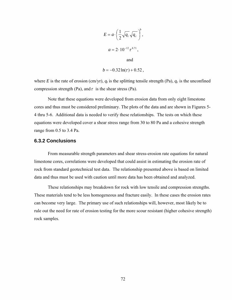
72

b

ct qqaE ⎟⎠⎞

⎜⎝⎛⋅=

21 ,

71.812102 τ−⋅=a ,

and

52.0)ln(32.0 +−= τb ,

where E is the rate of erosion (cm/yr), qt is the splitting tensile strength (Pa), qc is the unconfined

compression strength (Pa), andτ is the shear stress (Pa).

Note that these equations were developed from erosion data from only eight limestone

cores and thus must be considered preliminary. The plots of the data and are shown in Figures 5-

4 thru 5-6. Additional data is needed to verify these relationships. The tests on which these

equations were developed cover a shear stress range from 30 to 80 Pa and a cohesive strength

range from 0.5 to 3.4 Pa.

6.3.2 Conclusions

From measurable strength parameters and shear stress-erosion rate equations for natural

limestone cores, correlations were developed that could assist in estimating the erosion rate of

rock from standard geotechnical test data. The relationship presented above is based on limited

data and thus must be used with caution until more data has been obtained and analyzed.

These relationships may breakdown for rock with low tensile and compression strengths.

These materials tend to be less homogeneous and fracture easily. In these cases the erosion rates

can become very large. The primary use of such relationships will, however, most likely be to

rule out the need for rate of erosion testing for the more scour resistant (higher cohesive strength)

rock samples.

73

6.4 Future Work and Improvements

6.4.1 Continued Limestone Core Testing

Establishing the relationships between tensile and compressive rock strength parameters

and rates of erosion is a critical step towards developing methods for easily estimating erosion

rates in rock channel beds. By procuring more natural limerock cores from channel beds

throughout Florida, and testing these cores in the RETA, the curves for estimating erosion can be

enhanced. In the future, if there is significant variability between erosion rates and cohesive

strengths, a mean curve and standard deviation curves can be developed that will help to isolate

the expected erosion rates to a small range.

It would also be helpful to create Gatorock samples of high cohesive strength, and these

samples could be more efficiently compared to the existing curves. This would be useful in

quantifying any strength or erosion differences between naturally occurring rock particle

bonding and using cement to simulate this natural bonding.

6.4.2 Sand-Clay Mixtures

As described in Chapter 4 of this report, studying the erosion of sand-clay mixtures can

be useful for estimating erosion rate properties of sand clay mixtures. Sand –clay mixture

samples should be created using the procedure provided (or a variation thereof) and these

samples tested in the SERF to provide additional data.

6.4.3 Conversion to Manometers for Pressure Measurements in the SERF

One possible improvement to the SERF would be to replace or supplement the

differential pressure transducers with high resolution manometers. As a relatively inexpensive

and accurate method of pressure measurement, manometer tubes can be combined with computer

scanner technology to convert the monometer fluid elevations to voltages that can be read by the

data acquisition system.

74

REFERENCES

Annandale G.W., Smith S.P., Nairn R., Jones J.S., 1996. “Scour Power.” Journal of Civil Engineering, July, pp. 58-60.

Briaud, J., 1999. “Scour and Erosion Prediction,” p.1, http://tti.tamu.edu/geotech/scour/, last accessed July 7, 2006.

Cepero, C., 2002. “Insitu Rock Modulus.” Master’s Thesis, University of Florida.

Department of Natural Resources, Florida Gelogical Survey, Dept. of Environmental Regulation,1992. Florida’s Ground Water Quality Monitoring Program Background Geochemistry. pp. 13, 66, 69.

Gordon, S., 1991. “Scourability of Rock Formations.” Federal Highway Administration Memorandum, July 19, Washington, DC.

Hand, Randall S., 1998. “Development of a Cemented Sand Module for the Electronic Cone Penetrometer.” M.S. Report, University of Florida, Gainesville, Florida.

Henderson, M.R., 1999. “A Laboratory Method to Evaluate the Rates of Water Erosion of Natural Rock Materials.” M.S. Thesis, University of Florida, Gainesville, Florida.

Julien, Pierre Y., 1998. Erosion and Sedimentation. Cambridge University Press, pp. 213-221

Jumikis, A.R., 1983. Rock Mechanics. 2nd ed., TRANS TECH Publications, Clausthal-Zellerfeld, Federal Republic of Germany, pp. 37-45, 51-53.

Kerr, K.R., 2001. “A Laboratory Apparatus and Methodology for Testing Water Erosion in Rock Materials.” M.E. Thesis, University of Florida, Gainesville, Florida.

McNiel, J., Taylor, C., Lick, W., 1996. “Measurement of Erosion of Undisturbed Bottom Sedimnets with Depth.” ASCE Journal of Hydraulic Engineering, Vol. 122, Issue 6, pp. 316-324.

McVay, M.C., Townsend, F.C., Williams, R.C., October 1992. “Design Of Socketed Drilled Shafts In Limestone.” Journal of Geotechnical Engineering, Vol. 118, No. 10. pp. 1626-1637.

Mehta, A.J., In Press. “Sedimentation Engineering.” American Society of Civil Engineers Manuals on Enginering Practice #54. American Society of Civil Engineers, Reston, VA.

Mehta, A.J., McAnally, W.H., Hayter, E.J., Teeter, A.M., Schoellhamer, D., Heltzel, S.B., Carey, W.P., 1989. “Cohesive Sediment Transport.” ASCE Journal of HydraulicEngineering, Vol. 115, Issue 8, pp. 1076-1092.

75

Melville, B.W. and Chiew, Y.M., 1999. “Time Scale for Local Scour at Bridge Piers”, Journal of Hydraulic Engineering, ASCE, 125 (1), pp. 59-65.

Melville B.W., Coleman S.E., 2000. Bridge Scour. Water Resources Publications, LLC, Highlands Ranch, Colorado, USA.

Melville, B.W. and Sutherland, A.J., 1988. “Design Method for Local Scour at Bridge Piers”, Journal of Hydraulic Engineering, ASCE, 144 (10), pp. 1210-1226.

Ocean Engineering Associates, Inc., 2001. “Rock Scour Analysis for the I-10 Bridge Crossing of the Chipola River.” Report Submittal to the Florida Department of Transportation.

Pagan-Ortiz, J.E., 1998. “Status of the Scour Evaluation of Bridges over Waterways in the United States.” Proceedings of the International Water Resources Engineering Conference, Vol. 1, Water Resources Engineering 98, American Society of Civil Engineers, Memphis, TN, p.2.

Randazzo, A.F., Jones, D.S., 1997. The Geology of Florida. University Press of Florida, Gainesville, FL.

Richardson, E.V., Davis, S.R., 2001. “Evaluating Scour at Bridges.” 4th ed., Hydraulic Engineering Circular No. 18, Publication No. FHWA NHI 01-001, Office of Bridge Technology, Washington, DC.

Richardson, E.V., Davis, S.R., 1995. “Evaluating Scour at Bridges.” 3rd ed., Hydraulic Engineering Circular No. 18, Publication No. FHWA-IP-90-017, Office of Technology Applications, HTA-22, Washington, DC.

Roberts, J.D., James, S.C., Jepsen, R.A., 2003. “Measurements of Sediment Erosion and Transport with the ASSET Flume.” ASCE Journal of Hydraulic Engineering, Vol. 129, Issue 11, pp. 862-871.

Rokni, M., Olsson, C., Sunden, B., 1998. “Numerical and Experimental Investigation of Turbulent Flow in a Rectangular Duct.” International Journal for Numerical Methods in Fluids, Vol. 28, pp. 225-242.

Shepard, J.D., Frost, R., 1995. Failures in Civil Engineering: Structural, Foundation, and Geoenvironmental Case Studies. ASCE, New York, p.9.

Sheppard, D. Max, 2004. “Overlooked Local Sediment Scour Mechanism”, Transportation Research Record: Journal of the Transportation Research Board, No. 1890, TRB, National Research Council, Washington, D.C., 2004, pp. 107-111.

Sheppard, D. Max and Miller, William, July 1, 2006. “Live-Bed Local Pier Scour Experiments”, Journal of Hydraulic Engineering, ASCE, 132 (7), pp. 635-642.

76

Sheppard, D. Max; Odeh, Mufeed; Glasser, Tom, October 1, 2004. “Large Scale Clear-Water Local Pier Scour Experiments”, Journal of Hydraulic Engineering, ASCE, 130 (10), pp. 957-963.

Sleath, J.F.A., 1984. Sea Bed Mechanics. John Wiley & Sons, Inc., Cambridge., pp. 30-39, 260.

Van Rijn, L.C., 1993. Principles of Sediment Transport in Rivers, Estuaries, and Coastal Seas, Aqua Publications, Amsterdam. p. 4.1.

77

APPENDIX A PHOTOGRAPHS

Figure A-1 Photograph of the SERF at the University of Florida.

SERF control office is in the background.

78

Figure A-2 Photograph of the SERF pumps and valves.

79

Figure A-3 Front view of the SERF test cylinder with a sample raised into the flume.

Figure A-4 Photograph of the video camera and window at the back side of the SERF flume.

80

Figure A-5 Photograph of the RETA.

Figure A-5 Photograph of the RETA

81

Figure A-6 Front View of the RETA Cylinder with Sample and Torque-Measuring Load Cell.

Figure A-7 Gatorock molds secured to the rotating shaft device.

82

Figure A-8 Extracted Gatorock sample and mold for the RETA.

Figure A-9 From left to right: cemented sand molds for the RETA, the SERF, and an empty

mold.

83

Figure A-10 From front left to right: cemented sand molds for the SERF, the RETA, and an

empty mold. Extracted samples are seen at the back.

Figure A-11 Cemented sand sample failure in the RETA

84

APPENDIX B ADDITIONAL EXPERIMENTS

B.1 Description of Erosion of Expansive Clay Samples

Expansive clay samples were provided by the Florida Department of Transportation for

testing in the SERF. These samples were obtained from the intersection of Florida State Road 8

and Interstate 10, located in Jackson County, Florida. These samples were not taken from a

channel bed. The samples had a very high plasticity index and significantly increased in volume

when saturated. The procedure for extracting clay from Shelby tubes and testing cohesive

sediments in the SERF can be obtained from the SERF Operations Manual. The results and

observations for testing these expansive clays are presented later in this report.

B.1.1 Data

Figure C-1 presents the shear stress-erosion rate relationships observed in four expansive

clay cores from Jackson County. These samples were delivered sealed in Shelby tubes, and the

samples were extracted and tested in the SERF. Figure C-2 shows the automated advancement

behavior of the clay in the SERF over two tests at two shear stress values.

85

I-10 Jackson County Clay Erosion Rates vs Shear Stress

0.00

200.00

400.00

600.00

800.00

1000.00

1200.00

1400.00

1600.00

3.00 3.50 4.00 4.50 5.00 5.50 6.00 6.50

Shear Stress (Pa)

Eros

ion

Rat

e (m

/yr)

26-May

27-May

31-May

8-Jun

Linear (27-May)Power (26-May)

Power (31-May)

Power (8-Jun)

Figure C-1 Shear Stress-Erosion Rate Relationships for Similar Jackson County Clay

Samples.

86

I-10 Jackson County Clay Erosion Rate (2 Trials)

0

1

2

3

4

5

6

7

0 50 100 150 200 250

Time (min)

Sam

ple

Adv

ance

men

t (cm

)

4.2 Pa4.75 Pa

Figure C-2 Erosion Rate Behavior for Expansive Clay.

B.1.2 Results

This section addresses the portions of Chapter 4 and 5 pertaining to the erosion of an

expansive clay sample in the SERF. Although the clay material from the Jackson County site

appeared homogeneous to the naked eye, the erosion rate results from the SERF imply that these

materials are anything but consistent in composition. After testing the sample, it was discovered

that the clay samples provided were not extracted from a submersed location (from a channel

bed). From Figure 5-17, one can see the somewhat erratic behavior of sample at two different

shear stresses. During the beginning of a test at a specific shear stress, there was always an

initially large amount of erosion as the finer clay particles were transported from the test section.

Eventually, visual monitoring of the sample inside the SERF would reveal the exposure of a

large mass of harder clay. The larger mass acts as a clay particle with a large effective diameter.

Erosion rates would slow to a halt as all the fine clay particles surrounding the mass evacuate the

sample, and the acoustic sonar maintains the bed elevation because the chunk of clay maintains

an average elevation that is flush with the flume bed. As shown in Figure 5-17, by slightly

87

increasing the shear stress in the SERF, the large clay mass is able to lift into flow, indicating an

immediate large decrease in bed elevation to the SeaTek. The result is a return to drastic scour

of the finer particles with coarser particles occasionally being lifted into the flow and carried

downstream. Ultimately, the presence of durable clay masses of large effective particle diameter

will inhibit the SERF’s ability to advance the sample and accurately measure erosion rates.

Also, as expansive clays are subjected to saturation for any period of time, the expansion in the

clay reduces the shear stress required to initiate particle movement.

Also, the same figure reveals some sporadic bed elevation adjustments while attempting

to stabilize. In expansive clays, it has often been observed that the SERF raises the sample into

the line of flow. This occurs because the acoustic signal sent by the SeaTek is either scattered by

suspended clay particles or absorbed by the clay to a small degree before the signal bounces back

and returns to the SeaTek (indicating a deeper than actual bed elevation). In order to compensate

for this, the operator must apply an offset in the LabVIEW program to increase the depth of the

channel so as to maintain the sample surface flushness. That is, the program must be changed to

maintain the “effective surface” of the sample below the flume bed since the acoustic pulse is

penetrating the surface of the sample.

B.1.3 Conclusions

Because of the erratic behavior observed, testing heterogeneous or expansive clays in the

SERF can lead to subjective erosion rate results as the user must try to salvage any shear stress-

erosion rate relationship possible from a limited duration of adequate testing. Patches of stronger

cohesion or inter-particle bonding within the sample easily disrupt erosion testing and results in

wasted, untested lengths of valuable sample cores. Also, as the sample is exposed and given

time to saturate, the expansion reduces the shear stress required to initiate particle movement.

As these particular samples were not extracted directly from a channel bed, and given the

sensitive erosion and expansion behaviors observed in the samples, it is likely that these types of

clays are unable to stably exist in submerged environments where bridge piers may be placed.

There may, however, be situations where the channel is dry a high percentage of the time and

flood conditions only exist for a short duration and this information would be helpful For

88

example a highway overpass on an interstate highway that is only flooded during a 50 year event

and is dry otherwise.

B.2 Description of Dissolution of Limerock Experiment

One additional concern when measuring erosion rates at a bridge founded in limestone

rock is the potential for a natural chemical to influence the rate of scour. As many streams in

Florida and across the country are brown in color due to the presence of tannic acid, and as

rainfall and runoff may introduce acidic water into streams, it was hypothesized that this

chemical presence would increase the rate of limestone scour in a channel at some rate to be

determined. With an approximately known rate at which either lime molecules could be

expected to dissolve in dilute acids or as the bonds between limestone particles would weaken

and sever, a factor could be determined which could account for an increase in depth in a channel

bed. Referencing the Florida Geological Survey, it was determined that sulfuric acid and

carbonic acid from rainfall were the primary acids that could contribute to low pH levels in

streams in Florida. The maximum observed sulfate concentration in Florida rainwater is 22.8

mg/L with a median of 1.75 mg/L, and the drinking water limit is 250 mg/L. Carbonic acid, on

the other hand, has a stronger tendency to dissociate into bicarbonates. Although the

concentration of acid in rainfall is low and is not strong enough to play any significant role in

bed elevation lowering, a procedure for measuring the relationship between limerock erosion and

acid concentration is provided below (Department of Natural Resources, 1992).

B.2.1 Experimental Procedures

Five experimental procedures were developed for the determination of calcium carbonate

in limerock and the dissolution of limerock in carbonic and sulfuric acids under static and

dynamic conditions.

89

B.2.1.1 Determination of CaCO3 in Limerock

Mix solution of 2 M HCl by adding 166.66 ml of 12 molar HCl to one liter of deionized

water. Mix thoroughly and let sit for 5 minutes.

Weigh out 30 g of the 0.074 mm rock and place in a 750 ml beaker. Add 500 ml of the 1

M HCl and let reaction go to completion by allowing complete dissolution of the rock with the

use of a spin bar.

Take three 50 ml aliquots of the solution and transfer to 3 separate 150 ml Erlenmeyer

flask. Add 4 drops of phenolphthalein and back titrate with 2 M NaOH. The number of reacted

moles of HCl is assumed to be directly proportional to the percent of the CaCO3 in the rock.

This process should be repeated 2-3 times for accuracy.

B.2.1.2 Measurement of Lime Dissolution in Static Sulfuric Acid

Prepare a three liter solution of 1 M sulphuric acid.

Weigh out 30 grams of the 20 mm, 2 mm, 0.2 mm, and 0.074 mm rock and place in

separate 750 ml beakers. Add 500 ml of the 1 M sulfuric acid to all of the beakers in 5 min

intervals.

Take 25 ml aliquots every 15 minutes for back titration testing on a time scale. Add 2

drops of phenolphthalein and use the corresponding molarity for the NaOH back titration.

Repeat this process for the 0.1, 0.01, 0.001, 0.0001 molar solutions.

B.2.1.3 Measurement of Lime Dissolution in Dynamic Sulfuric Acid

Repeat the procedure listed above and add a spin bar to each beaker to keep the acid

flowing around the rock.

90

B.2.1.4 Measurement of Lime Dissolution in Static Carbonic Acid

Preparation of carbonic acid must be made in a pressure chamber of five or more

atmospheres. This is necessary in order to keep the carbonic acid from coming out of solution.

The experiment itself will also proceed inside a pressure chamber to determine the acidic effects

on the rock.

Weigh out 30 grams of the 20 mm, 2 mm, 0.2 mm, and 0.074 mm rock and place them in

different 750 ml beakers. Add 500 ml of the 1 M carbonic acid to all of the beakers in 5 min

intervals (if applicable determined by number of pressure chambers).

Take 25 ml aliquots every 15 minutes for back titration testing on a time scale. Add a

known amount of NaOH immediately to the aliquot as well as 2 drops of phenolphthalein and

use the corresponding molarity for the HCl for back titration.

Repeat this process for the 0.1, 0.01, 0.001, 0.0001 molar solutions.

B.2.1.5 Measurement of Lime Dissolution in Dynamic Carbonic Acid

Repeat the procedure listed above and add a spin bar to each beaker to keep the acid

flowing around the rock.

Information from the literature regarding the rates of limerock desolution in sulfuric and

carbonic acid in the concentrations found in Florida streams indicates that this may not be a

problem for durations of the normal like of a bridge (on the order of 75 to 100 years).

Experiments such as those described above, which are beyond the scope of this study, are needed

to answer these questions with confidence.

Rate of Erosion Properties of Rock and Clay€¦ · Final Report Rate of Erosion Properties of Rock...

Documents

Transcript of Rate of Erosion Properties of Rock and Clay€¦ · Final Report Rate of Erosion Properties of Rock...