Rapid Training of Information Extraction with Local and

Global Data Views

by

Ang Sun

A dissertation submitted in partial fulfillment

of the requirements for the degree of

Doctor of Philosophy

Department of Computer Science

New York University

May 2012

Professor Ralph Grishman

c© Ang Sun

All Rights Reserved, 2012

Dedicated to my wife and our son

iii

Acknowledgements

I would like to thank the following named entities: Ralph Grishman, Satoshi

Sekine, Heng Ji, Ernest Davis, Lakshminarayanan Subramanian, the Proteus Group,

and the Intelligence Advanced Research Projects Activity (IARPA). I would also

like to thank the following nominals: my wife, my parents, and my parents-in-law.

I would like to thank my advisor, Ralph Grishman, for his support throughout

of my PhD study at New York University. I thank Ralph for many hours of

discussions we had, for guiding me to separate the good ideas from the bad ones,

and for all the comments and suggestions he had for my papers including this

thesis. Without Ralph, this dissertation would not be possible. I especially thank

him for the Proteus T-shirt he gave as a gift to my baby son, Steven.

I thank Satoshi for being very supportive for my PhD study. I owe him a big

thanks for designing the awesome n-gram search tool that I used extensively at

NYU.

I would like to thank Heng for being willing to serve as an outside reader for

my thesis and for her constructive suggestions. Many thanks to the other two

members of my defense committee as well, Ernie and Lakshimi.

I would like to thank members of the Proteus Group. I enjoyed and benefited

a lot from the weekly group meeting.

This work is supported in part by the IARPA via Air Force Research Laboratory

(AFRL) contract number FA8650-10-C-7058. The U.S. Government is authorized

to reproduce and distribute reprints for Governmental purposes notwithstanding

any copy-right annotation thereon. The views and conclusions contained herein

are those of the author and should not be interpreted as necessarily representing

the official policies or endorsements, either expressed or implied, of IARPA, AFRL,

iv

or the U.S. Government.

I thank my parents and my parents-in-law for their selfless support of my PhD

study.

Lastly, I would like to thank my wife for her support and love, and for taking

care of our son, Steven.

v

Abstract

This dissertation focuses on fast system development for Information Extrac-

tion (IE). State-of-the-art systems heavily rely on extensively annotated corpora,

which are slow to build for a new domain or task. Moreover, previous systems

are mostly built with local evidence such as words in a short context window or

features that are extracted at the sentence level. They usually generalize poorly

on new domains.

This dissertation presents novel approaches for rapidly training an IE system

for a new domain or task based on both local and global evidence. Specifically, we

present three systems: a relation type extension system based on active learning,

a relation type extension system based on semi-supervised learning, and a cross-

domain bootstrapping system for domain adaptive named entity extraction.

The active learning procedure adopts features extracted at the sentence level as

the local view and distributional similarities between relational phrases as the global

view. It builds two classifiers based on these two views to find the most informative

contention data points to request human labels so as to reduce annotation cost.

The semi-supervised system aims to learn a large set of accurate patterns for

extracting relations between names from only a few seed patterns. It estimates

the confidence of a name pair both locally and globally : locally by looking at the

patterns that connect the pair in isolation; globally by incorporating the evidence

from the clusters of patterns that connect the pair. The use of pattern clusters

can prevent semantic drift and contribute to a natural stopping criterion for semi-

supervised relation pattern discovery.

For adapting a named entity recognition system to a new domain, we propose

a cross-domain bootstrapping algorithm, which iteratively learns a model for the

vi

new domain with labeled data from the original domain and unlabeled data from

the new domain. We first use word clusters as global evidence to generalize fea-

tures that are extracted from a local context window. We then select self-learned

instances as additional training examples using multiple criteria, including some

based on global evidence.

vii

Contents

Dedication . . . . . . . . . . . . . . . . . . . . . . . . . . . . . . . . . . . iii

Acknowledgements . . . . . . . . . . . . . . . . . . . . . . . . . . . . . . iv

Abstract . . . . . . . . . . . . . . . . . . . . . . . . . . . . . . . . . . . . vi

List of Figures . . . . . . . . . . . . . . . . . . . . . . . . . . . . . . . . . xii

List of Tables . . . . . . . . . . . . . . . . . . . . . . . . . . . . . . . . . xiii

1 Introduction 1

1.1 Named Entity Recognition . . . . . . . . . . . . . . . . . . . . . . . 2

1.1.1 Task . . . . . . . . . . . . . . . . . . . . . . . . . . . . . . . 2

1.1.2 Prior Work . . . . . . . . . . . . . . . . . . . . . . . . . . . 3

1.1.3 Cross-domain Bootstrapping for Named Entity Recognition . 8

1.2 Relation Extraction . . . . . . . . . . . . . . . . . . . . . . . . . . . 10

1.2.1 Task . . . . . . . . . . . . . . . . . . . . . . . . . . . . . . . 10

1.2.2 Prior Work . . . . . . . . . . . . . . . . . . . . . . . . . . . 11

1.2.3 Active and Semi-supervised Learning for Relation Type Ex-

tension . . . . . . . . . . . . . . . . . . . . . . . . . . . . . . 17

1.3 Outline of Thesis . . . . . . . . . . . . . . . . . . . . . . . . . . . . 20

2 Relation Type Extension: Active Learning with Local and Global

viii

Data Views 21

2.1 Introduction . . . . . . . . . . . . . . . . . . . . . . . . . . . . . . . 21

2.2 Task Definition . . . . . . . . . . . . . . . . . . . . . . . . . . . . . 24

2.3 The Local View Classifier . . . . . . . . . . . . . . . . . . . . . . . 25

2.4 The Global View Classifier . . . . . . . . . . . . . . . . . . . . . . . 27

2.5 LGCo-Testing . . . . . . . . . . . . . . . . . . . . . . . . . . . . . . 29

2.6 Baselines . . . . . . . . . . . . . . . . . . . . . . . . . . . . . . . . . 32

2.7 Experiments . . . . . . . . . . . . . . . . . . . . . . . . . . . . . . . 34

2.7.1 Experimental Setting . . . . . . . . . . . . . . . . . . . . . . 34

2.7.2 Results . . . . . . . . . . . . . . . . . . . . . . . . . . . . . . 35

2.7.3 Analyses . . . . . . . . . . . . . . . . . . . . . . . . . . . . . 37

2.8 Related Work . . . . . . . . . . . . . . . . . . . . . . . . . . . . . . 40

2.9 Conclusion . . . . . . . . . . . . . . . . . . . . . . . . . . . . . . . . 41

3 Relation Type Extension: Bootstrapping with Local and Global

Data Views 42

3.1 Introduction . . . . . . . . . . . . . . . . . . . . . . . . . . . . . . . 42

3.2 Pattern Clusters . . . . . . . . . . . . . . . . . . . . . . . . . . . . . 45

3.2.1 Distributional Hypothesis . . . . . . . . . . . . . . . . . . . 45

3.2.2 Pattern Representation - Shortest Dependency Path . . . . . 45

3.2.3 Pre-processing . . . . . . . . . . . . . . . . . . . . . . . . . . 46

3.2.4 Clustering Algorithm . . . . . . . . . . . . . . . . . . . . . . 47

3.3 Semi-supervised Relation Pattern Discovery . . . . . . . . . . . . . 48

3.3.1 Unguided Bootstrapping . . . . . . . . . . . . . . . . . . . . 48

3.3.2 Guided Bootstrapping . . . . . . . . . . . . . . . . . . . . . 51

3.4 Experiments . . . . . . . . . . . . . . . . . . . . . . . . . . . . . . . 53

ix

3.4.1 Corpus . . . . . . . . . . . . . . . . . . . . . . . . . . . . . . 53

3.4.2 Seeds . . . . . . . . . . . . . . . . . . . . . . . . . . . . . . . 54

3.4.3 Unsupervised Experiments . . . . . . . . . . . . . . . . . . . 55

3.4.4 Semi-supervised Experiments . . . . . . . . . . . . . . . . . 55

3.4.5 Evaluation . . . . . . . . . . . . . . . . . . . . . . . . . . . . 56

3.4.6 Results and Analyses . . . . . . . . . . . . . . . . . . . . . . 57

3.5 Related Work . . . . . . . . . . . . . . . . . . . . . . . . . . . . . . 59

3.6 Conclusions and Future Work . . . . . . . . . . . . . . . . . . . . . 60

4 Cross-Domain Bootstrapping for Named Entity Recognition 62

4.1 Introduction . . . . . . . . . . . . . . . . . . . . . . . . . . . . . . . 62

4.2 Related Work . . . . . . . . . . . . . . . . . . . . . . . . . . . . . . 65

4.3 Task and Domains . . . . . . . . . . . . . . . . . . . . . . . . . . . 66

4.4 Cross-Domain Bootstrapping . . . . . . . . . . . . . . . . . . . . . . 67

4.4.1 Overview of the CDB Algorithm . . . . . . . . . . . . . . . . 67

4.4.2 Seed Model Generalization . . . . . . . . . . . . . . . . . . . 68

4.4.3 Multi-Criteria-based Instance Selection . . . . . . . . . . . . 71

4.5 Experiments . . . . . . . . . . . . . . . . . . . . . . . . . . . . . . . 76

4.5.1 Data, Evaluation and Parameters . . . . . . . . . . . . . . . 76

4.5.2 Performance of the source Domain Model . . . . . . . . . . 78

4.5.3 Performance of the Generalized Model . . . . . . . . . . . . 79

4.5.4 Performance of CDB . . . . . . . . . . . . . . . . . . . . . . 80

4.6 Conclusion . . . . . . . . . . . . . . . . . . . . . . . . . . . . . . . . 82

5 Conclusion and Future Work 84

5.1 Conclusion . . . . . . . . . . . . . . . . . . . . . . . . . . . . . . . . 84

x

5.2 Future Work . . . . . . . . . . . . . . . . . . . . . . . . . . . . . . . 85

Bibliography 87

xi

List of Figures

1.1 NER Example in SGML format. . . . . . . . . . . . . . . . . . . . . 2

1.2 Example of un-supervised relation discovery. . . . . . . . . . . . . . 16

1.3 Example of the local view of a name pair. . . . . . . . . . . . . . . 19

1.4 Example of the global view of a name pair. Ci means the pattern

cluster i . . . . . . . . . . . . . . . . . . . . . . . . . . . . . . . . . 19

2.1 Precision-recall curve of LGCo-Testing. . . . . . . . . . . . . . . . . 38

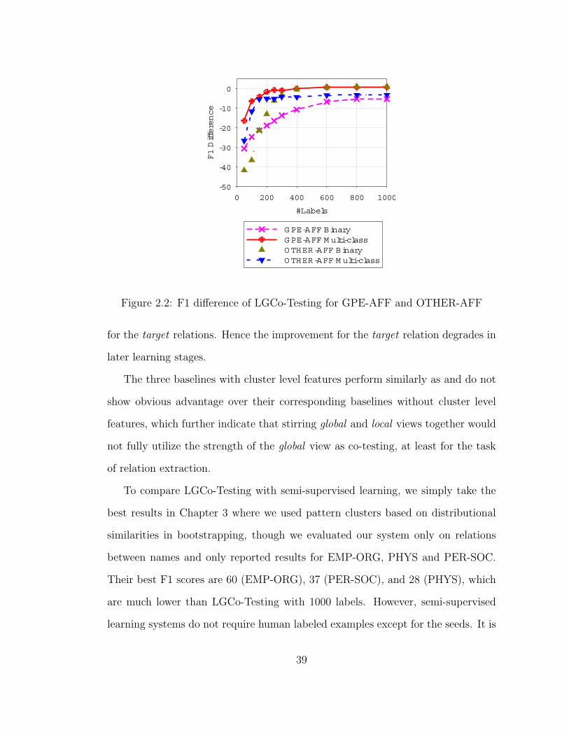
2.2 F1 difference of LGCo-Testing for GPE-AFF and OTHER-AFF . . 39

3.1 Shortest Dependency Path. . . . . . . . . . . . . . . . . . . . . . . 46

3.2 Precision-recall curve and Drift Rate for EMP/Located-in/SOC . . 58

4.1 Examples of NER task and domains . . . . . . . . . . . . . . . . . . 66

4.2 Performance of CDB . . . . . . . . . . . . . . . . . . . . . . . . . . 81

xii

List of Tables

1.1 NER Examples with BIO decoding scheme . . . . . . . . . . . . . . 4

1.2 Sample patterns that connect Bill Gates and Microsoft . . . . . . . 13

1.3 Sample name pairs that are connected by “, the chairman of ” . . . 14

1.4 Example of a pair of names that have multiple relation. . . . . . . . 15

2.1 ACE relation examples from the annotation guideline. Heads of

entity mentions are marked. . . . . . . . . . . . . . . . . . . . . . . 24

2.2 Sample local features for “<ei>President Clinton</ei> traveled to

<ej>the Irish border</ej> for an ... ” . . . . . . . . . . . . . . . . 26

2.3 7-gram queries for traveled to. . . . . . . . . . . . . . . . . . . . . . 28

2.4 Sample of similar relational phrases. . . . . . . . . . . . . . . . . . . 28

2.5 F1 difference (in percentage) = F1 of active learning minus F1 of

supervised learining. Bold numbers indicate the best performance.

UN := UncertaintyAL. SP := SPCo-Testing. LG := LGCo-Testing 36

3.1 Sample features for “X visited Y” as in “Jordan visited China” . . . 47

3.2 Seed patterns. . . . . . . . . . . . . . . . . . . . . . . . . . . . . . . 54

3.3 Top 15 patterns in the Located-in Cluster. . . . . . . . . . . . . . . 56

xiii

4.1 An example of words and their bit string representations. Bold ones

are transliterated Arabic words. . . . . . . . . . . . . . . . . . . . . 70

4.2 source domain data. . . . . . . . . . . . . . . . . . . . . . . . . . . 76

4.3 target domain data. . . . . . . . . . . . . . . . . . . . . . . . . . . . 77

4.4 Corpora for generating word clusters. . . . . . . . . . . . . . . . . . 77

4.5 Parameters for CDB. . . . . . . . . . . . . . . . . . . . . . . . . . . 78

4.6 Performance of source models over the 3 name types. . . . . . . . . 78

4.7 Performance of the generalized source model. . . . . . . . . . . . . . 79

xiv

Chapter 1

Introduction

Information Extraction (IE) is the task of extracting from texts instances of

predefined types of entities and relations involving these entities. This dissertation

studies the problem of rapid training of IE systems. We focus on two well-defined

IE tasks: Named Entity Recognition (NER) and Relation Extraction (RE). Pre-

vious state-of-the-art systems for these two tasks are typically trained with exten-

sively annotated corpora, making them hard to adapt to a new domain or extend

to a new task. These systems are categorized as supervised systems.

In contrast to the supervised approach, both semi-supervised and active learn-

ing approaches aim to reduce the amount of annotated data so as to speed up

the training of IE systems for new domains and new tasks. However, this brings

many new challenges. For example, how to prevent the well-known semantic drift

problem for the iterative process of semi-supervised learning? Can we find a good

and natural stopping criterion? What would be the most effective sample selection

method for active learning?

In the next two sections, we describe the two IE tasks, review the most relevant

1

previous work with emphasis on analyzing their shortcomings when applied to

new domains and tasks. And then we briefly introduce our solutions for domain

adaptation for NER and type extension for RE. The last section presents the

outline of this dissertation.

1.1 Named Entity Recognition

1.1.1 Task

NER, as an evaluation task, was first introduced in the Sixth Message Un-

derstanding Conference (MUC-6)[34]. Given a raw English text, the goal is to

identify names in it and classify them into one of the three categories: PERSON,

ORGANIZATION and LOCATION. For the example sentence in Figure1.1, an

NER system needs to extract Bill Gates as a PERSON, Seattle as a LOCATION,

and Microsoft as an ORGANIZATION. Other evaluations such as CoNLL[20], fol-

lowed MUC and extended it to many other languages other than English.

<PERSON>Bill Gates</PERSON>, born October 28, 1955 in <LOCATION>Seattle</LOCATION>, is the former chief executive officer (CEO) and currentchairman of <ORGANIZATION>Microsoft</ORGANIZATION>.

Figure 1.1: NER Example in SGML format.

Evaluation of NER performance is done by comparing system output against

answer keys prepared by a human annotator. We count as: correct if the NE tags

agree in both extent and type; spurious if a system tag does not match the tag

of the answer key; missing if a tag in the answer key has no matching tag in the

system output. We then compute recall, precision and F1 scores as follows:

2

recall =correct

correct+missing(1.1)

precision =correct

correct+ spurious(1.2)

F1 =2× recall × precision

recall + precision(1.3)

Note that the MUC evaluation gives partial credit to cases where a system NE

tag matched the answer key in extent but not in type, while the CoNLL scores

give no such partial credit. Following most previous work, we will use the CoNLL

evaluation metric instead of the MUC metric.

1.1.2 Prior Work

A comprehensive survey of NER is given by [61]. Here we only review the

classical NER models and other most relevant work of this dissertation.

1.1.2.1 Supervised NER

NER is well recognized as a sequence labeling task. Given a sequence of to-

kens/words of a sentence, T = (t1...tn), the goal is to assign it the most likely

sequence of name classes c1...cn. As a name may contain multiple tokens, it is

necessary and convenient to break a name class into a few subclasses. Table 1.1

shows an example using the BIO scheme, which splits a name type into B (begin-

ning of the name type) and I (continuation of the name type). A O tag is used to

represent a non-name token.

3

Bill Gates , born October 28 , 1955 in Seattle .B-person I-person O O O O O O O B-location O

Table 1.1: NER Examples with BIO decoding scheme

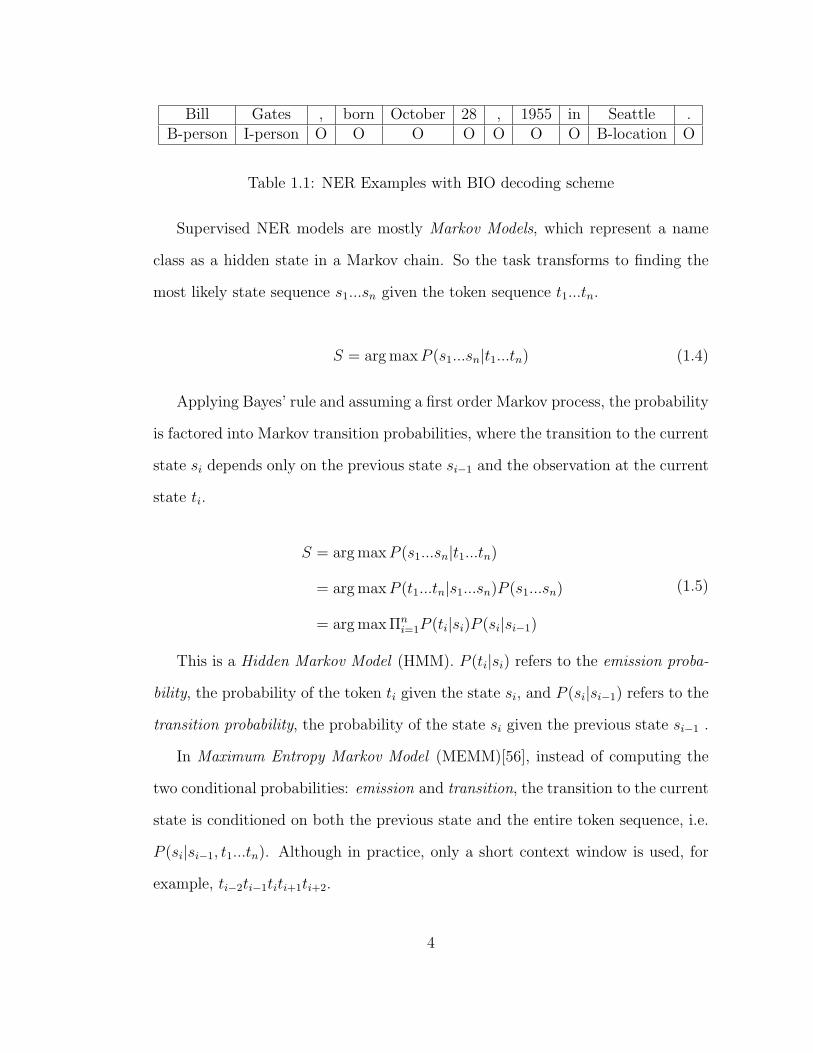
Supervised NER models are mostly Markov Models, which represent a name

class as a hidden state in a Markov chain. So the task transforms to finding the

most likely state sequence s1...sn given the token sequence t1...tn.

S = argmaxP (s1...sn|t1...tn) (1.4)

Applying Bayes’ rule and assuming a first order Markov process, the probability

is factored into Markov transition probabilities, where the transition to the current

state si depends only on the previous state si−1 and the observation at the current

state ti.

S = argmaxP (s1...sn|t1...tn)

= argmaxP (t1...tn|s1...sn)P (s1...sn)

= argmaxΠni=1P (ti|si)P (si|si−1)

(1.5)

This is a Hidden Markov Model (HMM). P (ti|si) refers to the emission proba-

bility, the probability of the token ti given the state si, and P (si|si−1) refers to the

transition probability, the probability of the state si given the previous state si−1 .

In Maximum Entropy Markov Model (MEMM)[56], instead of computing the

two conditional probabilities: emission and transition, the transition to the current

state is conditioned on both the previous state and the entire token sequence, i.e.

P (si|si−1, t1...tn). Although in practice, only a short context window is used, for

example, ti−2ti−1titi+1ti+2.

4

S = argmaxP (s1...sn|t1...tn)

= argmaxΠni=1P (si|si−1, t1...tn)

≈ argmaxΠni=1P (si|si−1, ti−2ti−1titi+1ti+2)

(1.6)

HMM and MEMM models can be quite effective when they are tested on the

same domain of texts as the training domain. However, they usually perform

poorly on a domain that is different or slightly different from the training domain.

For example, [21] reported that a system trained on the CoNLL 2003 Reuters

dataset achieved an F-measure of 0.908 when it was tested on a similar Reuters

corpus but only 0.643 on a Wall Street Journal dataset.

Looking closer at the domain effect problem, we observe that the models’ pa-

rameters (the transition probabilities of both the HMM and MEMM models and

the emission probability of the HMM model) are trained to optimize the perfor-

mance on domains that are similar to the training domain. A new domain may

contain many names and contexts that have not been observed by the models. An

unobserved token ti has poor parameter estimation, for example, the probability

that a state emits that token in an HMM model, P (ti|s). The transition from one

state to another will be poorly estimated as well, which is true for both HMM

and MEMM models. For example, using the BIO scheme, if the training domain

contains typical English person names (1 to 3 tokens) and the testing domain con-

tains many transliterated foreign names (more than 3 tokens), then the transition

probability from the state I-person to itself would be underestimated for the test-

ing domain, given that this type of transition is more frequent in the testing than

in the training domain.

To remedy this, supervised models would have to design sophisticated back-

5

off strategies[5]. Alternatively, one can annotate texts of the testing domain and

re-train the models. This however, is a time consuming process and may not be

reusable for other domains.

1.1.2.2 Semi-supervised NER

The portability of supervised NER models is limited by the availability of

annotated data of a new domain. Semi-supervised learning aims to build a model

for a new domain with only small amounts of labeled data and large amounts of

unlabeled data.

Semi-supervised NER is feasible because one can usually identify and classify

a name by either the name string itself (e.g., New York City), or by the context

in which the name appears (e.g., He arrived in <>). A bootstrapping procedure

based on the co-training [7] idea utilizes the name string itself and the context as

two views of a data point in NER. Starting with a few seed names of a particular

category, it first identifies and evaluates the contexts in which these names occur.

It then uses selected predictive and confident contexts to match new names which

are further used to learn new contexts.

Bootstrapping systems mostly focus on semantic lexicon acquisition [67][57][86],

building a dictionary of a specific semantic class from a few seed examples. The

evaluation is typically done by manually judging the correctness of the extracted

terms, usually only for the top ranked extractions. This accuracy-based evaluation

is quite different from the MUC and CoNLL evaluations. Only a few bootstrapping

systems used the MUC and CoNLL evaluation metrics[86]. Customizing these

systems for the MUC and CoNLL style within document NER is worth further

exploration.

6

A second problem with semi-supervised NER is semantic drift. While a name

typically belongs to just one class, there are names that belong to multiple classes

when they are separated from contexts (e.g., Washington can be a person or a

location). So bootstrapping for one class of names may extract names of other

classes. To alleviate this problem, seeds of multiple categories are introduced to

serve as negative categories to provide competition among categories[86]. However,

these negative categories are usually identified by hand, which undermines the

intention of semi-supervised learning which is to reduce human supervision.

More recently, [75] and [57] proposed to use unsupervised learning to discover

these negative classes. They cluster either words or contexts based on distributional

similarity and use identified clusters as negative classes so as to avoid the manual

construction of these classes.

A third problem with bootstrapping-based systems is the lack of a natural

stopping criterion. Most systems either use a fixed number of iterations or use a

labeled development set to detect the right stopping point. We propose to stop

bootstrapping by detecting semantic drift in Chapter 3. It is straightforward to

detect semantic drift if the bootstrapping process tends to accept more members

of the negative classes instead of the positive class.

1.1.2.3 Active Learning for NER

Active learning reduces annotation cost by selecting the most informative ex-

amples for requesting human labels. The most informative example can be the

most uncertain example tagged by the underlying NER model. However, selecting

uncertain examples may include a lot of outliers which are rare examples and may

not necessarily improve NER performance. [71] proposed a multiple-criteria-based

7

selection method, including informativeness, representativeness, density, and di-

versity, so as to maximize the performance gain one can achieve in a single round

of active learning by providing a good balance between selecting common instances

and rare instances.

Committee-based selection has also been applied to active learning for NER[47][4].

[4] builds two Markov models based on different feature sets ,uses KL-divergence to

quantify the disagreement between the two models, and select the most disagreed

examples to request human labels.

1.1.3 Cross-domain Bootstrapping for Named Entity Recog-

nition

Millions of dollars have already been spent on annotating news domain data and

state-of-the-art NER systems are typically trained with news data. However, these

supervised models perform poorly on non-news domains. Moreover, when building

a NER model for a new target domain, both semi-supervised and active learning

tend to work on the target domain directly and ignore the potential benefits one

can get from existing annotated news data.

We propose a cross-domain bootstrapping (CDB) algorithm to adapt a NER

model trained on a news domain to a terrorism report domain without annotating

examples on the latter. CDB first builds a MEMM model on the news domain,

iteratively tags a large unlabeled terrorism report corpus to select self-learned

labeled instances, and finally upgrades the model with these new instances. There

are two major components of CDB: feature generalization and instance selection.

Feature generalization. The news-trained model is based on English language

names, such as “John Smith” but is much less confident in extracting names from

8

other languages, such as “Abdul al-Fatah al-Jayusi”, which are more common in

US terrorism reports. To use the words from the names as features, our CDB algo-

rithm moves one level up to build word clusters and extracts clusters as features.

Specifically, words are clustered in a hierarchical way based on distributional sim-

ilarity. Words in terrorism reports may share the same cluster membership with

those in news articles. So even if the news-trained model does not include a specific

word of the terrorism report domain, the cluster level features may still fire for the

terrorism report domain.

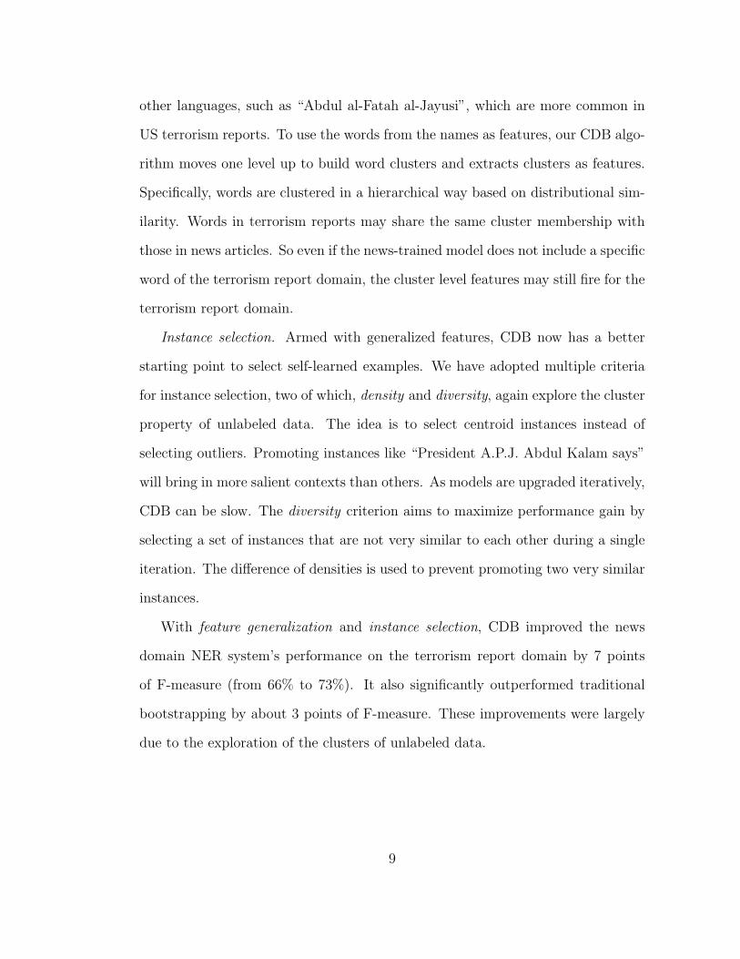
Instance selection. Armed with generalized features, CDB now has a better

starting point to select self-learned examples. We have adopted multiple criteria

for instance selection, two of which, density and diversity, again explore the cluster

property of unlabeled data. The idea is to select centroid instances instead of

selecting outliers. Promoting instances like “President A.P.J. Abdul Kalam says”

will bring in more salient contexts than others. As models are upgraded iteratively,

CDB can be slow. The diversity criterion aims to maximize performance gain by

selecting a set of instances that are not very similar to each other during a single

iteration. The difference of densities is used to prevent promoting two very similar

instances.

With feature generalization and instance selection, CDB improved the news

domain NER system’s performance on the terrorism report domain by 7 points

of F-measure (from 66% to 73%). It also significantly outperformed traditional

bootstrapping by about 3 points of F-measure. These improvements were largely

due to the exploration of the clusters of unlabeled data.

9

1.2 Relation Extraction

1.2.1 Task

Names and entities are isolated information. Connecting related entities and

labeling them with the right semantic relation type is the task of relation extrac-

tion, which would provide a more useful resource for IE-based applications. There

are two types of relation extraction tasks that have been extensively studied.

Relation mention extraction. The US government sponsored Automatic

Content Extraction (ACE) program introduced relation extraction in 2002 which

was continued until 2008. Table 2.1 shows the relation types and examples defined

in ACE 2004. ACE defines a relation over a pair of entities. And a relation mention

is defined over a pair of entity mentions in the same sentence. Assuming that the

sentence is “Adam, a data analyst for ABC Inc.”, there are two entities {Adam, a

data analyst} and {ABC Inc.} in it. Adam and a data analyst are two mentions

of the entity {Adam, a data analyst}. Relation mention is defined over the two

closest entity mentions in a sentence. So according to the ACE definition, an

EMPLOYMENT relation mention should be established between a data analyst

and ABC Inc. One needs to rely on coreference information to determine the

relation between Adam and ABC Inc.

Relation extraction between names. A large body of relation extraction

work concerns extracting relations between a pair of names, again in the same

sentence. So for the previous example, one needs to extract an EMPLOYMENT

relation between the two names Adam and ABC Inc. More recently, the Knowl-

edge Base Population (KBP) evaluation[42] introduces the task of slot filling, find-

ing attributes for PERSON and ORGANIZATION in about 1 million documents.

10

KBP does not constrain a relation to hold in a single sentence. In fact, for some

hard cases, one would have to do cross-sentence relation extraction to find certain

attributes.

Evaluation. As a relation extraction system relies on the output of an en-

tity extraction model, evaluating the performance of relation extraction is more

complicated than that of entity extraction. To make performance comparable

among different systems developed by different sites, researchers usually separate

the evaluation of entity extraction from relation extraction. For example, instead

of relying on system output of entity mentions, most reported ACE systems use

the hand annotated entity mentions as the input of a relation extraction system.

As for NER, relation extraction are usually evaluated based on precision, recall,

and f-measure.

1.2.2 Prior Work

1.2.2.1 Supervised relation extraction

A supervised approach casts relation extraction as a classification task. Given

a collection of documents that have been annotated with entities and relations, one

will build a positive example for a pair of entity mentions if the pair is annotated

with a type of relation, and build a negative example if the pair is not labeled with

any predefined relation types.

There are two standard learning strategies for relation extraction, flat and

hierarchical. The flat strategy simply trains a n+1 -way classifier for n classes

of relations and the non-relation class (no predefined relation holds for a pair

of entity mentions). The hierarchical strategy separates relation detection from

11

relation classification. It first trains a binary classifier which detects whether a

pair of entity mentions has a relation or not. Then a n-way classifier is trained to

distinguish among the n relation classes. This hierarchical strategy was proposed

based on the observation from the ACE corpora that the number of non-relation

instances is usually 8 to 10 times larger than that of relation instances. The

intention was to group all relation instances into one single class so as to alleviate

the effect of unbalanced class distribution between the relation and non-relation

classes and improve recall for relation instances.

Both feature-based and kernel-based classification apporaches have been ap-

plied to relation extraction.

A feature-based classifier starts with multiple level analyses, including tok-

enization, syntactic, and dependency parsing of the sentence that contains a pair

of entity mentions[48][93]. It then extracts a feature vector for the pair which con-

tains various entity, sequence, syntactic, and semantic features. Table 2.2 shows

an example feature set.

Pairs of entities that have the same relation type are usually connected by simi-

lar token sequences, the shortest paths in dependency trees, or have similar subtree

structures in syntactic parsing trees. These structures can be modeled as features

in a feature-based system but would be much more powerful if a kernel function

can be defined over them. In fact, kernel functions at the token sequence[14], de-

pendency path[13] and syntactic parsing tree[95] levels have all been proposed to

extract relations, with tree kernels working as effectively as or even better than a

feature-based system.

Both feature-based and kernel-based supervised relation extraction systems can

give state-of-the-art performance. However, extending such systems to a new type

12

of relation would require annotating data for this new type of relation from scratch.

This greatly impedes the application of such systems to extract a new type of

relation.

1.2.2.2 Semi-supervised relation extraction

Language is redundant. A pair of names may be connected by multiple patterns

(e.g., a sequence of tokens) that actually express the same relation. Table 1.2 shows

sample patterns that are all indicating that there is an EMPLOYMENT relation

between Bill Gates and Microsoft. Similarly, a single pattern may connect many

pairs of names. See the examples in Table 1.3.

Table 1.2: Sample patterns that connect Bill Gates and Microsoft

Using the pair of names as one view and the patterns connecting the pair as

another view, semi-supervised relation extraction usually adopts a co-training style

bootstrapping procedure[2]. It starts with a few seed patterns that indicate the

target relation to match name pairs and evaluate the confidence of these extracted

name pairs. Then in the next step it uses these name pairs to search for additional

patterns that are connecting these pairs. These newly discovered patterns are

13

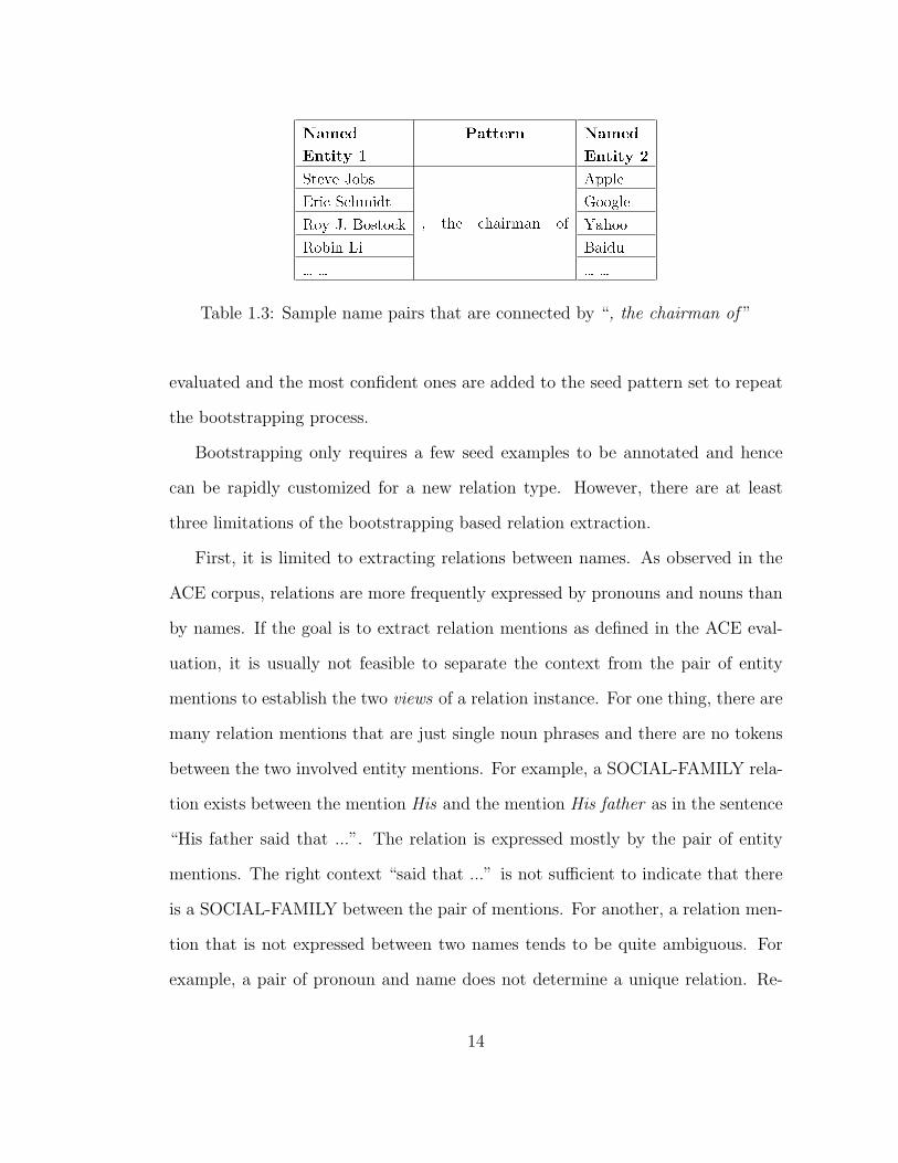
Table 1.3: Sample name pairs that are connected by “, the chairman of ”

evaluated and the most confident ones are added to the seed pattern set to repeat

the bootstrapping process.

Bootstrapping only requires a few seed examples to be annotated and hence

can be rapidly customized for a new relation type. However, there are at least

three limitations of the bootstrapping based relation extraction.

First, it is limited to extracting relations between names. As observed in the

ACE corpus, relations are more frequently expressed by pronouns and nouns than

by names. If the goal is to extract relation mentions as defined in the ACE eval-

uation, it is usually not feasible to separate the context from the pair of entity

mentions to establish the two views of a relation instance. For one thing, there are

many relation mentions that are just single noun phrases and there are no tokens

between the two involved entity mentions. For example, a SOCIAL-FAMILY rela-

tion exists between the mention His and the mention His father as in the sentence

“His father said that ...”. The relation is expressed mostly by the pair of entity

mentions. The right context “said that ...” is not sufficient to indicate that there

is a SOCIAL-FAMILY between the pair of mentions. For another, a relation men-

tion that is not expressed between two names tends to be quite ambiguous. For

example, a pair of pronoun and name does not determine a unique relation. Re-

14

placing the wild cards in “He * New York” with the pattern “lives in” will produce

a residence relation while with “drove to the city of” will give a locatedIn relation.

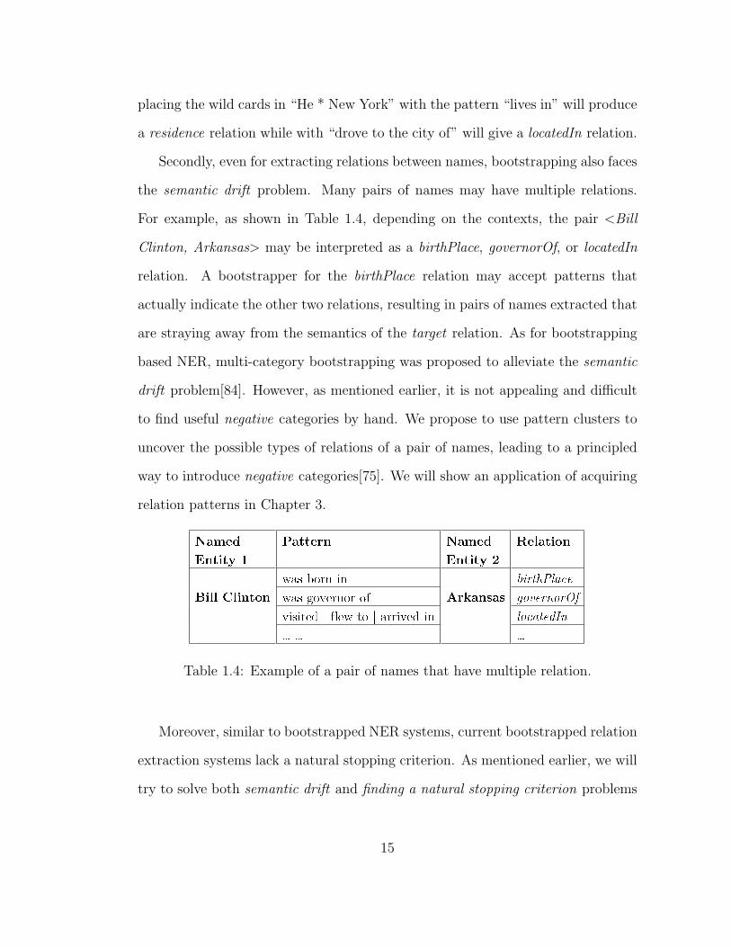
Secondly, even for extracting relations between names, bootstrapping also faces

the semantic drift problem. Many pairs of names may have multiple relations.

For example, as shown in Table 1.4, depending on the contexts, the pair <Bill

Clinton, Arkansas> may be interpreted as a birthPlace, governorOf, or locatedIn

relation. A bootstrapper for the birthPlace relation may accept patterns that

actually indicate the other two relations, resulting in pairs of names extracted that

are straying away from the semantics of the target relation. As for bootstrapping

based NER, multi-category bootstrapping was proposed to alleviate the semantic

drift problem[84]. However, as mentioned earlier, it is not appealing and difficult

to find useful negative categories by hand. We propose to use pattern clusters to

uncover the possible types of relations of a pair of names, leading to a principled

way to introduce negative categories[75]. We will show an application of acquiring

relation patterns in Chapter 3.

Table 1.4: Example of a pair of names that have multiple relation.

Moreover, similar to bootstrapped NER systems, current bootstrapped relation

extraction systems lack a natural stopping criterion. As mentioned earlier, we will

try to solve both semantic drift and finding a natural stopping criterion problems

15

at the same time.

1.2.2.3 Un-supervised relation extraction

Both supervised and semi-supervised approaches extract instances of relations

of predefined types. Relations can be also discovered in an un-supervised way. The

main idea is to cluster pairs of names based on the similarity of context words that

are intervening between the names. Figure 1.2 shows one example from [37]. Like

semi-supervised learning, it also utilizes the linguistic intuition that name pairs

that have the same relation usually share similar contexts.

�������������� ������� ���������� ������

���� ��������������������

������ �����

�����������������

������� �� ���� ��

��������������

�

������� ������������������������

�� ������

����� ���� ��

���� �����

�

������ �������� ���� ��!������� ������"

#����������

������

Figure 1.2: Example of un-supervised relation discovery.

The relation discovery procedure begins with named entity tagging. Then the

contexts of a pair of names are gathered together to generate a feature vector.

The similarity between pairs of names is calculated using the cosine measure,

which is used as the distance measure of Complete Linkage, a type of Hierarchical

Agglomerative Clustering, to cluster pairs of names.

Un-supervised relation discovery can discover meaningful relations with zero

annotation cost. However, it faces a few challenges to be more beneficial to poten-

16

tial applications. First of all, as mentioned earlier in this chapter, a pair of names

may actually exhibit multiple relation types. This might affect the consistency of

the labels of some of the generated relation clusters. Secondly, further improve-

ments are needed for better alignment between generated clusters and a specific

application. For example, one application might need the governor relation while

another might need all relations that are related to government officials. Generat-

ing clusters at the right level of granularity with respect to the specific underlying

application need further exploration.

1.2.3 Active and Semi-supervised Learning for Relation

Type Extension

This dissertation studies how to rapidly and accurately extend a system for a

new type of relation. To reduce annotation cost, we apply two learning algorithms

for fast training of relation extraction systems: active learning and semi-supervised

learning. In both approaches, we show that one can benefit from using both the

local view and the global view of a relation instance to reduce annotation cost

without degrading the performance of relation extraction. We briefly introduce

our approaches below and will present their details in Chapter 2 and 3.

1.2.3.1 Active learning for relation type extension

We apply active learning to extract relation mentions, as defined in the ACE

program. The local view involves the features extracted at the sentence level (from

a sentence that contains a pair of entity mentions). As it is not reasonable to

separate the pair of entity mentions and their context to establish two data views,

we represent each relation instance as a relational phrase. Roughly speaking, we

17

define a relational phrase as the following: if there are no context tokens between

the two mentions, we treat the two mentions together as a relational phrase. If

there are tokens in between, we then use the middle token sequence as the rela-

tional phrase. We will give a formal definition of relational phrase in Chapter 2.

The global view involves the distributional similarity between relational phrases

computed from a 2-billion-token text corpus.

We build a feature-based relation classifier based on the local view. We also

build a k-nearest neighbor classifier based on the global view, classifying an unla-

beled instance based on its closest labeled examples. We then measure the degree

of disagreement between the two classifiers using KL-divergence. The instances

with the largest degree of deviation between the two classifiers are treated as the

most informative examples to request human labels.

1.2.3.2 Semi-supervised learning for relation type extension

We apply semi-supervised learning to extract relations between names. Specif-

ically, we develop a bootstrapping procedure for acquiring semantic patterns for

extracting a target relation.

The procedure begins with a small set of patterns of the target relation to match

name pairs. These name pairs should be evaluated based on their confidence of

indicating the target relation. Traditional bootstrapping evaluates the confidence

of a newly matched name pair by looking at the confidence of each individual

pattern that connects the name pair in isolation. We call this type of confidence

the local view confidence. This dissertation moves one level up to build pattern

clusters and estimates the confidence of a name pair based on the clusters of

patterns that connect the name pair as well. We call it the global view confidence.

18

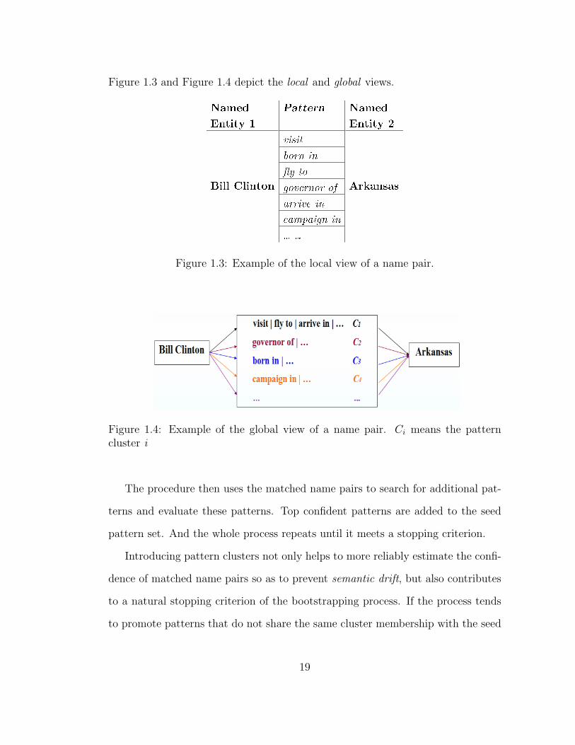
Figure 1.3 and Figure 1.4 depict the local and global views.

Figure 1.3: Example of the local view of a name pair.

Figure 1.4: Example of the global view of a name pair. Ci means the patterncluster i

The procedure then uses the matched name pairs to search for additional pat-

terns and evaluate these patterns. Top confident patterns are added to the seed

pattern set. And the whole process repeats until it meets a stopping criterion.

Introducing pattern clusters not only helps to more reliably estimate the confi-

dence of matched name pairs so as to prevent semantic drift, but also contributes

to a natural stopping criterion of the bootstrapping process. If the process tends

to promote patterns that do not share the same cluster membership with the seed

19

patterns, then it is likely that patterns being accepted are actually indicating other

types of relations other than the target relation. Hence semantic drift occurs and

the process should be stopped.

1.3 Outline of Thesis

The rest of the dissertation is organized as follows: Chapter 2 presents in

detail the proposed active learning based relation type extension with local and

global data views. Chapter 3 focuses on the bootstrapping based relation type

extension with local and global data views[75]. We then present the cross-domain

bootstrapping algorithm for domain adaptive NER in Chapter 4[77]. We conclude

and point to future work in Chapter 5.

20

Chapter 2

Relation Type Extension: Active

Learning with Local and Global

Data Views

2.1 Introduction

Relation extraction aims to connect related entities and label them with the

right semantic relationship. For example, a relation extraction system needs to

detect an Employment relation between the entities He and Arkansas in the sen-

tence He was the governor of Arkansas. The task of relation type extension is to

extend an existing relation extraction system to be able to extract a new type of

relation, often called the target relation, preferably in a fast, cheap and accurate

way.

A supervised approach can tackle this problem in an accurate way. But it

is slow and expensive as it relies on human annotation of a large quantity of

21

examples. Semi-supervised learning, in contrast, does not require much human

effort by automatically bootstrapping a system for the target relation from only a

few labeled examples and a large unlabeled corpus. However, a large gap still exists

between the performance of semi-supervised and supervised systems. Moreover,

their performance largely depends on the choice of seeds[81][50].

Another attractive alternative is active learning, which reduces annotation cost

by requesting labels of only the most informative examples while maintaining high

learning performance. It is also shown to be robust to the choice of the seeds[47].

Specifically, we focus on relation type extension with co-testing[60], an active learn-

ing approach in the co-training[7] setting. It minimizes human annotation effort

by building two classifiers based on two different views of the data and asking for

human labels only for contention data points, points on which the two classifiers

disagree about their labels. The key to the success of co-testing is to find a natural

way of splitting a data point into two views that are uncorrelated and compatible

(each view is sufficient in labeling the data point).

To date, there is limited work on applying co-testing to relation type extension.

The main difficulty, as we believe, is the lack of a natural way of partitioning the

data into two uncorrelated and compatible views. Unlike named entity classification

where one can rely on either the name string itself (Arkansas) or the context (was

the governor of <>) to determine the type of the named entity[23][47], the type of

a relation is mostly determined by the context in which the two entities appear. For

example, it is not possible to decide the type of relation between He and Arkansas

without the local context was the governor of. If the context was traveled to, then

the relation of the two entities would change entirely. Thus it is not desirable to

separate the entities from their context to establish two views. Instead, we treat

22

them together as a single view, the local view.

Motivated by the idea of distributional similarity, we move beyond the local

view to interpret the relation between two entities. Specifically, we compute from

a 2 billion token corpus the distributional similarities between relational phrases.

We take these similarities as the global view upon which we build a classifier which

classifies new examples based on the k−nearestneighbor algorithm. For example,

if the phrase arrived in is more similar to traveled to than to was the governor

of, the global view classifier classifies entities connected by arrived in as the same

relation as those connected by traveled to. Armed with this global view classifier

and a classifier trained with features extracted from the local view, applying co-

testing to relation type extension becomes feasible.

The main contributions of active learning with local and global views are: it

indeed introduces two uncorrelated and compatible views for relation extraction. It

provides substantial reduction of annotation effort as compared to various baselines

based on an extensive experimental study on the ACE 2004 corpus. Furthermore,

it leads to faster convergence of learning.

The next section introduces our task. Section 2.3 and 2.4 describes the local

and global view classifiers in detail. We present LGCo-Testing and baseline systems

in Section 2.5 and 2.6, and evaluate them in Section 2.7. We discuss related work

in Section 2.8 and conclude this chapter in Section 2.9.

23

2.2 Task Definition

We choose to work on the well defined relation extraction task of the ACE1

program in 2004, mostly driven by the purpose of system comparison as many

published results on this data set are available. A relation is defined over a pair

of entities within a single sentence. ACE 2004 defined 7 major relation types.

Some examples from the annotation guideline2 are shown in Table 2.1. Following

previous work, we only deal with relation mentions.

Table 2.1: ACE relation examples from the annotation guideline. Heads of entitymentions are marked.

We consider two experimental settings to simulate real world settings when we

build a system for a target relation.

1. Binary setting where we treat one of the ACE relation types as the target

relation. We use as labeled data a few labeled examples of the target relation

(possibly by random selection). And all other examples in the ACE corpus

are treated as unlabeled data.

2. Multi-class setting where we treat one of the ACE relations as the target rela-

1Task definition: http://www.itl.nist.gov/iad/894.01/tests/ace/ ACE guidelines:http://projects.ldc.upenn.edu/ace/

2http://projects.ldc.upenn.edu/ace/docs/EnglishRDCV4-3-2.PDF

24

tion and all others as auxiliary relations. We use as labeled data a few labeled

examples of the target relation and all labeled auxiliary relation examples.

All other examples in the ACE corpus are treated as unlabeled data. This

multi-class setting simulates a common training scenario where one wants to

extend a system trained with the extensive annotation of the ACE relation

types to additional types of relations.

2.3 The Local View Classifier

There are two common learning approaches for building a classifier based on

the local view: feature based[48][93][45] and kernel based[88][13][14][92][95]. As we

want to compare LGCo-Testing with co-testing based on a feature split at the local

level, we choose to build a feature based local classifier.

Given a relation instance x = (s, ei, ej), where ei and ej are a pair of entities

and s is the sentence containing the pair, the local classifier starts with multiple

level analyses of the sentence such as tokenization, syntactic parsing, and depen-

dency parsing. It then extracts a feature vector v which contains a variety of

lexical, syntactic and semantic features for each relation instance. Our features

are cherrypicked from previous feature based systems. Table 2.2 shows the feature

set with examples.

After feature engineering, the local classifier applies machine learning algo-

rithms to learn a function which can estimate the conditional probability p(c|v),the probability of the type c given the feature vector v of the instance x. We used

maximum entropy (MaxEnt) to build a binary classifier (for the binary setting)

and a multi-class classifier (for the multi-class setting) because the training is fast,

25

Table 2.2: Sample local features for “<ei>President Clinton</ei> traveled to<ej>the Irish border</ej> for an ... ”

26

which is crucial for active learning as it is not desirable to keep the annotator

waiting because of slow training.

2.4 The Global View Classifier

Building a classifier based on the global view involves three stages of process:

extracting relational phrases, computing distributional similarities, and building

the classifier based on similarities. We describe these stages in detail below.

Extracting relational phrases. Given a relation instance x = (s, ei, ej) and

assuming that ei appears before ej, we represent it as a relational phrase px, which

is defined as the n-gram that spans the head3 of ei and that of ej. Formally,

px=[head ei,head ej]. For example, we extract Clinton traveled to the Irish border

as the phrase for the example in Table 2.2. As our goal is to collect the tokens

before and after a phrase as features to capture the similarity between phrases and

long phrases are too sparse to be useful, we instead use the definition px = (ei, ej)

(tokens between ei and ej) when the phrase contains more than 5 tokens. Thus

for the example in Table 2.2, because the previously extracted phrase contains 6

tokens, we will instead use the phrase “traveled to” to represent that instance.

Computing distributional similarities. We first compile our 2 billion token

text corpus to a database of 7-grams[70] and then form 7-gram queries to extract

features for a phrase. Example queries for the phrase “traveled to” are shown in

Table 2.3.

We then collect the tokens that could instantiate the wild cards in the queries

as features. Note that tokens are coupled with their positions. For example, if the

3The last token of a noun group.

27

Table 2.3: 7-gram queries for traveled to.

matched 7-gram is President Clinton traveled to the Irish border, we will extract

from it the following five features: President -2, Clinton -1, the +1, Irish +2 and

border +3.

Each phrase P is represented as a feature vector of contextual tokens. To weight

the importance of each feature f, we first collect its counts, and then compute an

analogue of tf-idf : tf as the number of corpus instances of P having feature f

divided by the number of instances of P ; idf as the total number of phrases in the

corpus divided by the number of phrases with at least one instance with feature

f. Now the token feature vector is transformed into a tf-idf feature vector. We

compute the similarity between two vectors using Cosine similarity. The most

similar phrases of traveled to and his family are shown in Table 2.4.

Table 2.4: Sample of similar relational phrases.

Building the classifier. We build the global view classifier based on the k-

28

nearest neighbor idea, classifying an unlabeled example based on closest labeled

examples. The similarity between an unlabeled instance u and a labeled instance

l is measured by the similarity between their phrases, pu and pl. Note that we

also incorporate the entity type constraints into the similarity computation. The

similarity is defined to be zero if the entity types of u and l do not match. The

similarity between u and a relation type c, sim(u, c), is estimated by the similarity

between u and its k closest instances in the labeled instance set of c (we take the

averaged similarity if k > 1; we will report results with k = 3 as it works slightly

better than 1, 2, 4 and 5). Let h(u) be the classification function, we define it as

follows:

h(u) = argmaxc

sim(u, c) (2.1)

2.5 LGCo-Testing

We first introduce a general co-testing procedure, then describe the details of

the proposed LGCo-Testing.

Let DU denote unlabeled data, and DL denote labeled data, the co-testing

procedure repeats the following steps until it converges:

1. Train two classifiers h1 and h2 based on two data views with DL

2. Label DU with h1 and h2 and build a contention set S

3. Select S̄ ⊆ S based on informativeness and request human labels

4. Update: DL = DL ∪ S̄ and DU = DU\S̄

Initialization. Initialization first concerns the choice of the seeds. For the

multi-class setting, it also needs to effectively introduce the instances of auxiliary

29

relations.

For the choice of the seeds, as we are doing simulated experiments on the ACE

corpus, we take a random selection strategy and hope multiple runs of our exper-

iments can approximate what will actually happen in real world active learning.

Moreover, it was empirically found that active learning is able to rectify itself from

bad seeds[47]. In all experiments for both the binary and the multi-class settings,

we use as seeds 5 randomly selected target relation instances and 5 randomly se-

lected non-relation instances (entity pairs in a sentence not connected by an ACE

relation).

For the multi-class setting, we use a stratified strategy to introduce the auxil-

iary relation instances: the number of selected instances of a type is proportional

to that of the total number of instances in the labeled data. We also make the

assumption that our target relation is as important as the most frequent auxil-

iary relation and select these two types equally. For example, assuming that we

only have two auxiliary types with 100 and 20 labeled instances respectively, we

will randomly select 5 instances for the first type and 1 instance for the second

type, given that we initialized our active learning with 5 target relation seeds. We

also experimented with several other ways in introducing the auxiliary relation

instances and none of them were as effective as the stratified strategy. For one ex-

ample, using all the auxiliary instances to train the initial classifiers unfortunately

generates an extremely unbalanced class distribution and tends to be biased to-

wards the auxiliary relations. For another, selecting the same number of instances

for the target relation type and all the auxiliary types does not take full advantage

of the class distribution of the auxiliary types, which can be estimated with the

labeled data pool.

30

Informativeness measurement. It is straightforward to get the hard labels

of an instance from both the local and global view classifiers. As the local classifier

uses MaxEnt which is essentially logistic regression, we take the class with the

highest probability as the hard label. The hard label of the global classifier is the

relation type to which the instance is most similar. As long as the two classifiers

disagree about an instance’s hard label and one of the labels is our target relation,

we add it to the contention set.

Quantifying the disagreement between the two classifiers is not as straightfor-

ward as getting the hard labels because the local classifier produces a probability

distribution over the relation types while the global classifier produces a similar-

ity distribution. So we first use the following formula to transform similarities to

probabilities.

p(c|u) = exp(sim(u, c))∑i exp(sim(u, ci))

(2.2)

Here u is an instance that needs to be labeled, c is a specific relation type, and

sim(u, ci) is the similarity between u and one of the relation types ci.

We then use KL-divergence to quantify the degree of deviation between the

two probability distributions. KL-divergence measures the divergence between

two probability distributions p and q over the same event space χ:

D(p||q) =∑

x∈χp(x) log

p(x)

q(x)(2.3)

It is non-negative. It is zero for identical distributions and achieves its max-

imum value when distributions are peaked and prefer different labels. We rank

the contention instances by descending order of KL-divergence and pick the top 5

31

instances to request human labels during a single iteration.

It is worth mentioning that, for each iteration in the multi-class setting, aux-

iliary instances are introduced using the stratified strategy as in the initialization

step.

Convergence detection. We stop LGCo-Testing when we could not find

contention instances.

2.6 Baselines

We compare our approach to a variety of baselines, including six active learning

baselines, one supervised system and one semi-supervised system. We present the

details of active learning baselines below, and refer the reader to the experiment

section to learn more about other baselines.

SPCo-Testing. One of the many competitive active learning approaches is

to build two classifiers based on a feature split at the local level. As reported

by[45], either the sequence features or the parsing features are generally sufficient

to achieve state-of-the-art performance for relation extraction. So we build one

classifier based on the sequence view and the other based on the parsing view. More

precisely, one classifier is built with the feature set based on {entity, sequence} and

the other based on {entity, syntactic parsing, dependency parsing}. We build these

two classifiers with MaxEnt. The initialization is the same as in LGCo-Testing.

KL-divergence is used to quantify the disagreement between the two probability

distributions returned by the two MaxEnt classifiers. Contention points are ranked

in descending order of KL-divergence and the top 5 ones are used to query the

annotator in one iteration. Like LGCo-Testing, SPCo-Testing stops when the

32

contention set is empty.

UncertaintyAL. This is an uncertainty-based active learning baseline. We

build a single MaxEnt classifier based on the full feature set in Table 2.2 at the

local level. It uses the same initialization as in LGCo-Testing. Informativeness

measurement is based on uncertainty, which is approximated by the entropy h(p)

of the probability distribution of the MaxEnt classifier over all the relation types

ci.

h(p) = −∑

i

p(ci) log p(ci) (2.4)

It is also non-negative. It is zero when one relation type is predicted with a

probability of 1. It attains its maximum value when the distribution is a uniform

one. So the higher the entropy, the more uncertain the classifier is. So we rank

instances in descending order of entropy and pick the top 5 ones to request human

labels. Stopping UncertaintyAL cannot be naturally done as with co-testing. A

less appealing solution is to set a threshold based on the uncertainty measure.

RandomAL. This is a random selection based active leaning baseline. 5 in-

stances are selected randomly during a single iteration. There is no obvious way to

stop RandomAL although one can use a fixed number of instances as a threshold,

a number that might be related to the budget of a project.

The next three baselines aim to investigate the benefits of incorporating fea-

tures from the global view into the local classifier. They are inspired by recent

advances in using cluster level features to compensate for the sparseness of lexi-

cal features[59][76]. Specifically, we use the distributional similarity as a distance

measure to build a phrase hierarchy using Complete Linkage. The threshold for

cutting the hierarchy into clusters is determined by its ability to place the initial

33

seeds into a single cluster. We will revisit how the threshold is selected in Chapter

3. For extracting cluster level features, take traveled to as an example, if its cluster

membership is c, we will extract a cluster feature phraseCluster = c.

UncertaintyAL+. The only difference between UncertaintyAL+ and Uncer-

taintyAL is its incorporation of cluster features in building its classifier. This is

essentially the active learning approach presented by [59].

SPCo-Testing+. It differs from SPCo-Testing only in its sequence view clas-

sifier, which is trained with additional phrase cluster features.

LGCo-Testing+. It differs from LGCo-Testing only in its local view classifier,

which is trained with additional phrase cluster features.

2.7 Experiments

2.7.1 Experimental Setting

We experiment with the nwire and bnews genres of the ACE 2004 data set,

which are benchmark evaluation data for relation extraction. There are 4374 rela-

tion instances and about 45K non-relation instances. Documents are preprocessed

with the Stanford parser4 and chunklink5 to facilitate feature extraction. Note

that following most previous work, we use the hand labeled entities in all our

experiments.

We do 5-fold cross-validation as most previous supervised systems do. Each

round of cross-validation is repeated 10 times with randomly selected seeds. So,

a total of 50 runs are performed (5 subsets times 10 experiments). We report

4http://nlp.stanford.edu/software/lex-parser.shtml5http://ilk.uvt.nl/team/sabine/chunklink/README.html

34

average results of these 50 runs. Note that we do not experiment with the DISC

(discourse) relation type which is syntactically different from other relations and

was removed from ACE after 2004.

The size of unlabeled data is approximately 36K instances (45K ÷ 5 × 4).

Each iteration selects 5 instances to request human labels and 200 iterations are

performed. So a total of 1,000 instances are presented to our annotator. This

setting simulates satisfying a customer’s demand for an adaptive relation extractor

in a few hours. Assuming two entities and their contexts (the annotation unit) are

highlighted and an annotator only needs to mark it as a target relation or not, 4

instances per minute should be a reasonable or underestimated annotation speed.

And assuming that our annotator takes a 10-minute break in every hour, he or she

can annotate 200 instances per hour. We are now ready to test the feasibility and

quality of relation type extension in a few hours.

2.7.2 Results

We evaluate active learning on the target relation. Penalty will be given to

cases where we predict target as auxiliary or non-relation, and vice versa. To

measure the reduction of annotation cost, we compare active learning with the

results of [76], which is a state-of-the-art feature-based supervised system. We

use the number of labeled instances to approximate the cost of active learning.

So we list in Table 2.5 the F1 difference between an active learning system with

different number of labeled instances and the supervised system trained on the

entire corpus.

The results of LGCo-Testing are simply based on the local classifier’s predic-

tions on the test set. For the SPCo-Testing system, a third classifier is trained with

35

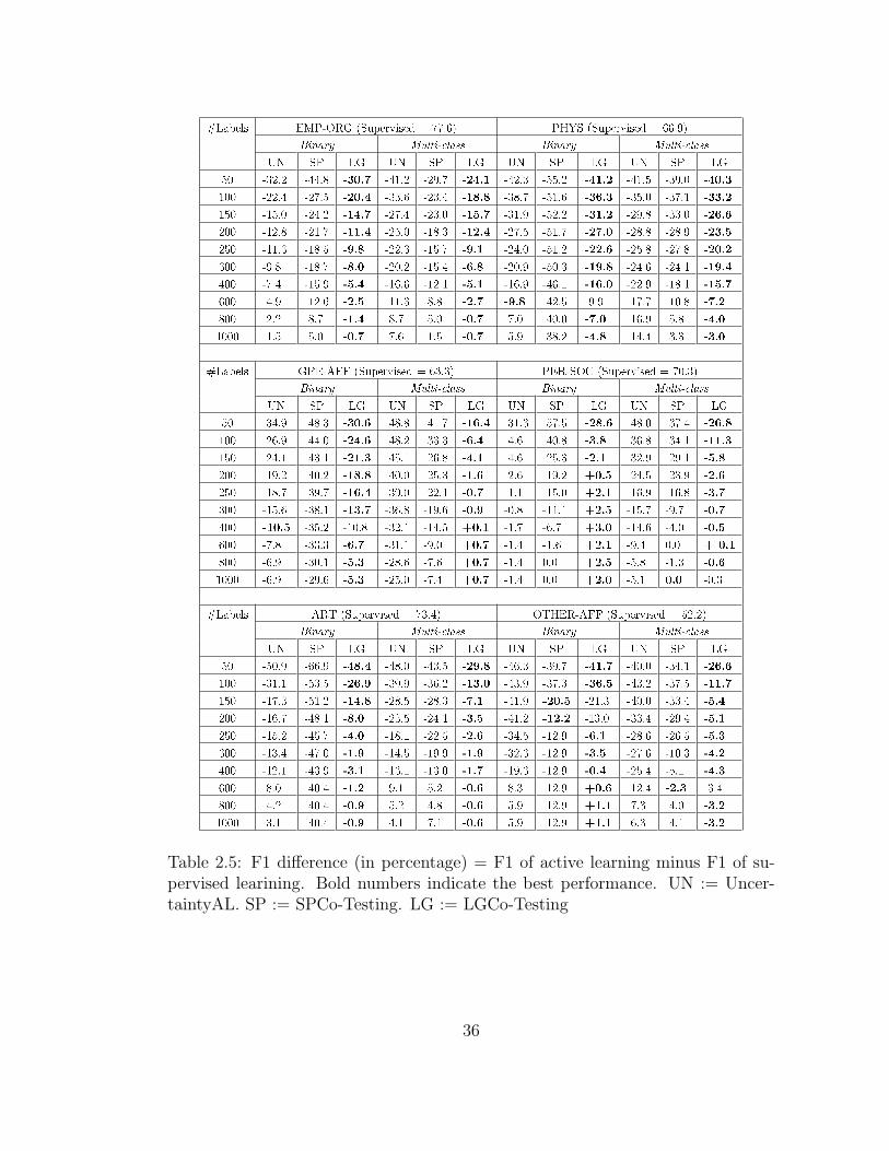
Table 2.5: F1 difference (in percentage) = F1 of active learning minus F1 of su-pervised learining. Bold numbers indicate the best performance. UN := Uncer-taintyAL. SP := SPCo-Testing. LG := LGCo-Testing

36

the full feature set to get test results. As there is a large gap between RandomAL

and the supervised system (40% F1 difference regardless of the number of labeled

instances), it is excluded from Table 2.5. The three baselines with cluster level fea-

tures perform similarly as their corresponding baselines without cluster phrases,

e.g. UncertaintyAL+ and UncertaintyAL perform similarly. So we exclude their

results too.

2.7.3 Analyses

Comparing active learning with supervised learning: LGCo-Testing trained

with 1,000 labeled examples achieves results comparable to supervised learning

trained with more than 35K labeled instances in both the binary and themulti-class

settings. This is true even for the two most frequent relations in ACE 2004, EMP-

ORG and PHYS (about 1.6K instances for EMP-ORG and 1.2K for PHYS). This

represents a substantial reduction in instances annotated of 97%. So assuming our

annotation speed is 200 instances per hour, we can build in five hours a competitive

system for EMP-ORG and a slightly weak system for PHYS. Moreover, we can

build comparable systems for the other four relations in less than 5 hours. Much of

the contribution, as depicted in Figure 2.1, can be attributed to the sharp increase

in precision during early stages and the steady improvement of recall in later stages

of learning.

Comparing active learning systems: the clear trend is that LGCo-Testing out-

performs UncertaintyAL and SPCo-Testing by a large margin in most cases for

both experimental settings. This indicates its superiority in selective sampling for

fast system development and adaptation. SPCo-Testing, which is based on the

feature split at the local level, does not consistently beat the uncertainty based

37

Recall

10 20 30 40 50 60 70 80 90Precision

0

10

20

30

40

50

60

70

80

90

EM P-ORGPER-SOCARTOTHER-AFFGPE-AFFPHYS

Figure 2.1: P-R curve of LGCo-Testing with the multi-class setting. Each dotrepresents one iteration.

systems. Part of the reason, as we believe, is that the sequence and parsing views

are highly correlated. For example, the token sequence feature “traveled to” and

the dependency path feature “nsubj’ traveled prep to” are hardly conditionally

independent.

Comparing LGCo-Testing in the multi-class setting with that in the binary

setting, we observe that the reduction of annotation cost by incorporating auxiliary

types is more pronounced in early learning stages (#labels < 200) than in later

ones, which is true for most relations. Figure 2.2 depicts this by plotting the F1

difference (between active learning and supervised learning) of LGCo-Testing in the

two experimental settings against the number of labels. Besides the two relations

GPE-AFF and OTHER-AFF shown in Figure 2.2, taking ART as a third example

relation type, with 50 labels, the F1 difference of the multi-class LGCo-Testing is

-29.8 while the binary one is -48.4, which represents a F1 improvement of 19.6 when

using auxiliary types. As the number of labels increases, the multi-class setting

incorporates more and more auxiliary instances, which might decrease the priors

38

#Labels

0 200 400 600 800 1000

F1 Difference

-50

-40

-30

-20

-10

0

GPE-AFF BinaryGPE-AFF M ulti-class OTHER-AFF BinaryOTHER-AFF M ulti-class

Figure 2.2: F1 difference of LGCo-Testing for GPE-AFF and OTHER-AFF

for the target relations. Hence the improvement for the target relation degrades in

later learning stages.

The three baselines with cluster level features perform similarly as and do not

show obvious advantage over their corresponding baselines without cluster level

features, which further indicate that stirring global and local views together would

not fully utilize the strength of the global view as co-testing, at least for the task

of relation extraction.

To compare LGCo-Testing with semi-supervised learning, we simply take the

best results in Chapter 3 where we used pattern clusters based on distributional

similarities in bootstrapping, though we evaluated our system only on relations

between names and only reported results for EMP-ORG, PHYS and PER-SOC.

Their best F1 scores are 60 (EMP-ORG), 37 (PER-SOC), and 28 (PHYS), which

are much lower than LGCo-Testing with 1000 labels. However, semi-supervised

learning systems do not require human labeled examples except for the seeds. It is

39

impressive that with just a few seeds, semi-supervised learning can achieve F1 of

60 for the EMP-ORG relation. Combing it with active learning to further reduce

the annotation cost is definitely a promising research avenue of our future work.

2.8 Related Work

To the best of our knowledge, this is the first piece of work in using active

learning for relation type extension and the literature on this topic is rather limited.

Our work is first motivated by co-training[7] and co-testing[60] which provide us

with a solid theoretical foundation.

Our global view is mostly triggered by recent advances in using cluster level

features for generalized discriminative models, including using word clusters[59]

and phrase clusters[54] for name tagging and using word clusters for relation

extraction[16][76].

Ourmulti-class setting is similar to the transfer learning setting of Jiang (2009),

namely building up a system for a target relation with a few target instances and all

auxiliary instances. They removed auxiliary instances from their evaluation data

while we preserved auxiliary instances in our evaluation data, which unfortunately

hinders a direct and fair comparison between their system and ours.

Perhaps the most relevant work is the our semi-supervised learning system

in Chapter 3 which uses pattern clusters as an additional view for an enhanced

confidence measure of learned name pairs. The two works differ in specific learning

approaches and how the global view is used.

40

2.9 Conclusion

We have presented LGCo-Testing, a multi-view active learning approach for

relation type extension based on local and global views. Evaluation results showed

that LGCo-Testing can reduce annotation cost by 97% while maintaining the per-

formance level of supervised learning. It has prepared us well to apply active learn-

ing to real world relation type extension tasks. Combining it with semi-supervised

learning to further reduce annotation cost is another promising research avenue.

41

Chapter 3

Relation Type Extension:

Bootstrapping with Local and

Global Data Views

3.1 Introduction

The Natural Language Processing (NLP) community faces new tasks and new

domains all the time. Without enough labeled data of a new task or a new domain

to conduct supervised learning, semi-supervised learning is particularly attractive

to NLP researchers since it only requires a handful of labeled examples, known as

seeds. Semi-supervised learning starts with these seeds to train an initial model;

it then applies this model to a large volume of unlabeled data to get more la-

beled examples and adds the most confident ones as new seeds to re-train the

model. This iterative procedure has been successfully applied to a variety of NLP

tasks, such as hypernym/hyponym extraction[38], word sense disambiguation[87],

42

question answering[66], and information extraction[11][23][67][2][85][19].

While semi-supervised learning can give good performance for many tasks, it is

a procedure born with two defects. One is semantic drift. When semi-supervised

learning is under-constrained, the semantics of newly promoted examples might

stray away from the original meaning of seed examples as discussed in [11][24][15].

For example, a semi-supervised learning procedure to learn semantic patterns for

the Located-in relation (PERSON in LOCATION/GPE) might accept patterns

for the Employment relation (employee of GPE/ORGANIZATION) because many

unlabeled pairs of names are connected by patterns belonging to multiple relations.

Patterns connecting <Bill Clinton, Arkansas> include Located-in patterns such as

“visit”, “arrive in” and “fly to”, but also patterns indicating other relations such

as “governor of”, ”born in”, and “campaign in”. Similar analyses can be applied to

many other examples such as <Bush, Texas> and <Schwarzenegger, California>.

Without careful design, semi-supervised learning procedures usually accept bogus

examples during certain iterations and hence the learning quality degrades.

The other shortcoming of semi-supervised learning is its lack of natural stopping

criteria. Most semi-supervised learning algorithms either run a fixed number of

iterations[2] or run against a separate labeled test set to find the best stopping

criterion[1]. The former solution needs a human to keep eyeballing the learning

quality of different iterations and set ad-hoc thresholds accordingly. The latter

requires a separate labeled test set for each new task or domain. They make semi-

supervised learning less appealing than it could be since the intention of using

semi-supervised learning is to minimize supervision.

In this chapter, we propose a novel learning framework which can automatically

monitor the semantic drift and find a natural stopping criterion for semi-supervised

43

learning. Central to our idea is that instead of using unlabeled data directly

in semi-supervised learning, we first cluster the seeds and unlabeled data in an

unsupervised way before conducting semi-supervised learning. The semantics of

unsupervised clusters are usually unknown. However, the cluster to which the seeds

belong can serve as the target cluster. Then we guide the semi-supervised learning

procedure using the target cluster. Under such learning settings, semantic drift

can be automatically detected and a stopping criterion can be found: stopping the

semi-supervised learning procedure when it tends to accept examples belonging to

clusters other than the target cluster.

We demonstrate in this chapter the above general idea by considering a boot-

strapping procedure to discover semantic patterns for extracting relations between

named entities based on both local and global data views.

Traditional bootstrapping usually starts with some high-precision and high fre-

quency seed patterns for a specific relation to match named entities. It evaluates

the confidence of a newly matched name pair by looking at the confidence of each

individual pattern that connects the name pair in isolation. We call this type of

confidence the local view confidence. This dissertation presents a novel bootstrap-

ping that moves one level up to build pattern clusters and estimates the confidence

of a name pair based on the clusters of patterns as well. We call it the global view

confidence. Using pattern clusters leads to a more reliable confidence estimation

of a pair of named entities. Moreover, it uncovers that a pair of named entities

might be connected by patterns indicating multiple relations by assuming that

different clusters of patterns indicating different types of relations. We should give

these pairs of names lower confidence. We then use newly promoted named entities

to search for additional confident patterns connecting them. When patterns that

44

are being promoted have different cluster memberships from the seed patterns,

semantic drift occurs and we should stop the bootstrapping process.

The next section describes our unsupervised pattern clusters. Section 3.3

presents the details of our novel bootstrapping procedure based on local and global

data views. We evaluate our algorithms in Section 3.4 and present related work in

Section 3.5. We draw conclusions and point to future work in Section 3.6.

3.2 Pattern Clusters

3.2.1 Distributional Hypothesis

The Distributional Hypothesis[36] states that words that tend to occur in sim-

ilar contexts tend to have similar meanings. [53] extended this hypothesis to cover

patterns (dependency paths in their case). The idea of the extension is that if two

patterns tend to occur in similar contexts then the meanings of the patterns tend

to be similar. For example, in “X solves Y” and “X finds a solution to Y”, “solves”

and “finds a solution to” share many common Xs and Y s and hence are similar to

each other. This extended distributional hypothesis serves as the basis on which

we compute similarities for each pair of patterns.

3.2.2 Pattern Representation - Shortest Dependency Path

We adopt a shortest dependency path (SDP) representation of relation pat-

terns. SDP has demonstrated its power in kernel methods for relation extraction[13].

Its capability in capturing most of the information of interest is also evidenced by a

systematic comparison of effectiveness of different information extraction patterns

45

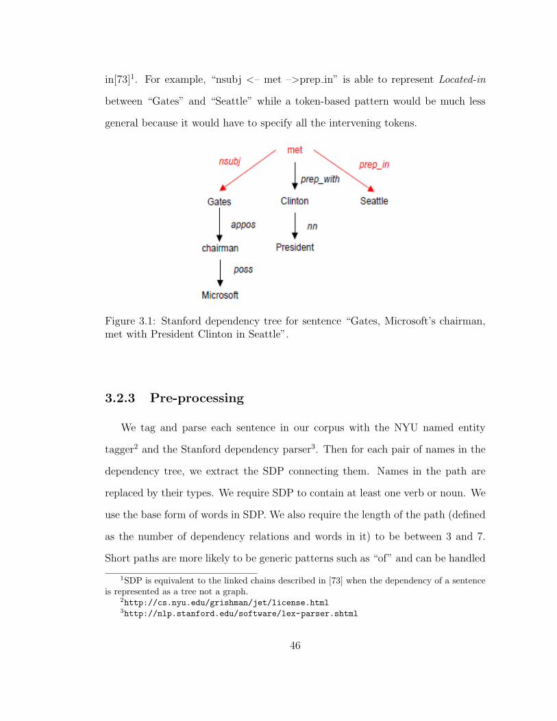
in[73]1. For example, “nsubj <– met –>prep in” is able to represent Located-in

between “Gates” and “Seattle” while a token-based pattern would be much less

general because it would have to specify all the intervening tokens.

Figure 3.1: Stanford dependency tree for sentence “Gates, Microsoft’s chairman,met with President Clinton in Seattle”.

3.2.3 Pre-processing

We tag and parse each sentence in our corpus with the NYU named entity

tagger2 and the Stanford dependency parser3. Then for each pair of names in the

dependency tree, we extract the SDP connecting them. Names in the path are

replaced by their types. We require SDP to contain at least one verb or noun. We

use the base form of words in SDP. We also require the length of the path (defined

as the number of dependency relations and words in it) to be between 3 and 7.

Short paths are more likely to be generic patterns such as “of” and can be handled

1SDP is equivalent to the linked chains described in [73] when the dependency of a sentenceis represented as a tree not a graph.

2http://cs.nyu.edu/grishman/jet/license.html3http://nlp.stanford.edu/software/lex-parser.shtml

46

separately as in[62]. Very long paths are more likely to be non-relation patterns

and too sparse to be useful even if they are relation patterns.

3.2.4 Clustering Algorithm

The basic idea of our clustering algorithm is to group all the paths (including

the seed paths used later for semi-supervised learning) in our corpus into different

clusters based on distributional similarities. We first extract a variety of features

from the named entities X and Y connected by a path P as shown in Table 3.1.

We then compute an analogue of tf-idf for each feature f of P as follows: tf

as the number of corpus instances of P having feature f divided by the number

of instances of P ; idf as the total number of paths in the corpus divided by the

number of paths with at least one instance with feature f . Then we adopt a vector

space model, i.e., we construct a tf-idf feature vector for each P . Now we compute

the similarity between two vectors/paths using Cosine similarity and cluster all

the paths using Complete Linkage.

Feature Type ExampleName Type of X LEFT PERSONName Type of Y RIGHT GPE

Combination of Types of X and Y PERSON GPEConjunction of String and Type of X LEFT Jordan PERSONConjunction of String and Type of Y RIGHT China GPE

Conjunction of Strings and Types of X and Y Jordan PERSON China GPE

Table 3.1: Sample features for “X visited Y” as in “Jordan visited China”

Some technical details deserve more attention here.

Feature extraction: We extract more types of features than the DIRT para-

phrase discovery procedure used in [53]. [53] considered X and Y separately while

47

we also use the conjunction of X and Y . We also extract named entity types as

features since we are interested in discovering relations among different types of

names. Some names are ambiguous such as Jordan. We hope coupling the type

with the string of the name may alleviate the ambiguity.

Similarity measure and clustering method: There are many ways to

compute the similarity/distance between two feature vectors, such as Cosine, Eu-

clidean, Hamming, and Jaccard coefficient. There are also many standard clus-

tering algorithms. Our choice of the Cosine similarity measure and the Complete

Linkage clustering algorithm are mostly driven by that they are the most popular

similarity measure and clustering algorithm in NLP applications.

3.3 Semi-supervised Relation Pattern Discovery

We first present a standard bootstrapping algorithm which evaluates the con-

fidence of a name pair based on local evidence only. And we call it unguided

bootstrapping. Then we describe our new bootstrapping procedure whose confi-

dence measure for name pairs is based on both local and global evidence. We call

this guided bootstrapping because of the use of pattern clusters for better evaluating

the confidence of name pairs and for detecting the stopping criterion.

3.3.1 Unguided Bootstrapping

The procedure associates a precision between 0 and 1 with each pattern, and

a confidence between 0 and 1 with each name pair. Initially the seed patterns for

a specific relation R have precision 1 and all other patterns 0. It consists of the

following steps:

48

Step1: Use seed patterns to match new NE pairs and evaluate NE

pairs.

Intuitively, for a newly matched NE pair , if many of the k patterns connecting

the two names are high-precision patterns then the name pair has a high confidence.

The confidence is computed by the following formula.

Conf(Ni) = 1−k∏

j=1

(1− Prec(pj)) (3.1)

Problem: While the intuition is correct, in practice this will over-rank NE pairs

which are not only matched by patterns belonging to the target relation R but are

also connected by patterns of many other relations. This is because of the initial

settings used in many semi-supervised learning systems: seeds are assigned high

confidence. Thus all NE pairs matched by initial seed patterns will have very high

confidence.

Suppose the target relation is Located-in, and “visited” is a seed pattern; then

the <Clinton, Arkansas> example will be over-rated because we cannot take into

account that it would also match patterns of other relations such as governorOf

and birthPlace in a real corpus. This will cause a vicious circle, i.e., bogus NE

pairs extract more bogus patterns which further extract more bogus NE pairs.

We believe this flaw of the initial settings partially results in the semantic drift

problem.

The problem happens because we are looking at the patterns that connect a

name pair in isolation. If we insist to use only the local view to evaluate a name

pair, i.e., by looking at the patterns in isolation, one can imagine that the problem

can not be solved by using a different formula to replace the one presented here. A

49

possible solution is to study the structure of unlabeled data (NE pairs in our case)

and integrate this structure information into the initial settings. Indeed, this is

where pattern clusters come into play. We will demonstrate this in Section 3.3.2.

Step 2: Use NE pairs to search for new patterns and rank patterns.

Similar to the intuition in Step 1, for a pattern p, if many of the NE pairs it

matches are very confident then p has many supporters and should have a high

ranking. We can use formula 3.2 to estimate the confidence of patterns and rank

them.

Conf(p) =Sup(p)

|H| log Sup(p) (3.2)

Here |H| is the number of unique NE pairs matched by p and Sup(p) is the sum

of the support it can get from the |H| pairs:

Sup(p) =

|H|∑

j=1

Conf(Nj) (3.3)

The precision of p is given by the average confidence of the NE pairs matched

by p. Formula 3.4 normalizes the precision to range from 0 to 1. As a result the

confidence of each NE pair is also normalized to between 0 and 1.

Prec(p) =Sup(p)

|H| (3.4)

Step 3: Accept patterns

Most systems accept the K top ranked patterns in Step 2 as new seeds, subject

to some restrictions such as requiring the differences of confidence of theK patterns

to be within a small range.

Step 4: Loop or stop

50

The procedure now decides whether to repeat from Step 1 or to terminate.

Most systems simply do not know when to stop. They either run a fixed number

of iterations or use some held-out data to find one criterion that works the best

for the held-out data.

3.3.2 Guided Bootstrapping

Recall that our clustering algorithm in Section 3.2 provides us with K clusters,

each of which contains n (n differs in different clusters) patterns. Every pattern

in our corpus now has a cluster membership (the seed patterns have the same

membership).

The most important benefit from our pattern clusters is that now we can mea-

sure how strongly a NE pair Ni is associated with our target cluster Ct (the one

to which the seed patterns belong).

Prob(Ni ∈ Ct) =

∑p∈Ct

freq(Ni, p)

m(3.5)

Here freq(Ni, p) is the number of times p matches Ni and m is the total number

of pattern instances matching Ni.

We integrate this prior cluster distribution of each NE pair into the initial

settings of our new bootstrapping procedure.

Step1: Use seed patterns to match new NE pairs and evaluate NE

pairs.

Assumption: A good NE pair must be strongly associated with the target

cluster and can be matched by multiple high-precision patterns. In other words,

it has to have strong support from both the global and local evidence.

51

So we evaluate a NE pair by the harmonic mean of two confidence scores,

namely the global confidence as its association with the target cluster and the local

confidence given by the patterns matching it.

Conf(Ni) =2× Local Conf(Ni)×Global Conf(Ni)

Local Conf(Ni) +Global Conf(Ni)(3.6)

Local Conf(Ni) = 1−k∏

j=1

(1− Prec(pj)) (3.7)

Global Conf(Ni) = Prob(Ni ∈ Ct) (3.8)

Under such settings, <Clinton, Arkansas> will be assigned a lower confidence

score for the Located-in relation than it is in the unguided bootstrapping. Even if

we assign high precision to our seed patterns such as “visited” and consequently

the Local Conf is very high, it can still be discounted by the Global Conf . The

Global Conf of <Clinton, Arkansas> related to the Located-in relation is indeed

very low (less than 0.1) in our experiments.

Step 2: Use NE pairs to search for new patterns and rank patterns.

All the measurement functions are the same as those used in the unguided

bootstrapping. However, with better ranking of NE pairs in Step 1, the patterns

are also ranked better than they are in the unguided bootstrapping.

Step 3: Accept patterns

We also accept the K top ranked patterns.

Step 4: Loop or stop

Since each pattern in our corpus has a cluster membership, we can monitor

the semantic drift easily and naturally stop: it drifts when the procedure tries to

52

accept patterns which do not belong to the target cluster; we can stop when the

procedure tends to accept more patterns outside of the target cluster.

If our clustering algorithm can give us perfect pattern clusters, we can stop

bootstrapping immediately after it accepts the first pattern not belonging to the

target cluster. Then the bootstrapping becomes redundant since all it does is to

consume the patterns of the target cluster.

Facing the reality of the behavior of many clustering algorithms, we allow the

procedure to occasionally accept patterns outside of the target cluster but we are

not tolerant when it tries to accept more patterns outside of the target cluster

than patterns in it. Note that when such patterns are accepted they will be moved

to the target cluster and invoke the re-computation of Global Conf of NE pairs

connected by these patterns. The ranking functions in step 1 and 2 insure that the

procedure will only accept patterns which can gain strong support from NE pairs

that are strongly associated with the target cluster and are connected by many

confident patterns.

3.4 Experiments

3.4.1 Corpus

Our corpora contain 37 years of news articles: TDT5, NYT(94-00), APW(98-

00), XINHUA(96-00), WSJ(94-96), LATWP(94-97), REUFF(94-96), REUTE(94-

96), and WSJSF(87-94). It contains roughly 65 million sentences and 1.3 billion

tokens.

53

3.4.2 Seeds

Seeds of the 3 relations we are going to test are given in table 3.2. Located-in

detects relation between PERSON and LOCATION/GPE; Social (SOC ) detects

social relations (either business or family) between PERSON and PERSON; Em-

ployment (EMP) detects employment relations between PERSON and ORGANI-

ZATION.

Table 3.2: Seed patterns.

(nsubj, dobj, prep, appos, poss, nsubjpass, agent stand for subject, direct ob-

ject, preposition, apposition, possessive, passive nominal subject and complement

of passive verb). The quote marks in Table 3.2 and Table 3.3 denote inverse de-

pendencies in the dependency path. We provide more seeds (executives and staff)

for EMP because it has been pointed out in [74] that EMP contains a lot of job

titles.

We work on these three relations mainly because of the availability of bench-

mark evaluation data. These are the most frequent relations in our evaluation

54

data.

3.4.3 Unsupervised Experiments

We run the clustering algorithm described in Section 3.2 using all the 37 years’

data. We require that a pattern match at least 7 distinct NE pairs and that an

NE pair must be connected by at least 7 unique patterns. As a result, there are

635,128 patterns (22,225 unique ones) used in experiments. We use 0.005 as the

cutoff threshold of Complete Linkage. The threshold is decided by trying a series

of thresholds and searching for the maximal4 one that is capable of placing the seed

patterns for each relation into a single cluster. Table 3.3 shows the top 15 patterns

(ranked by their corpus frequency) of the cluster into which our Located-in seeds

fall.

3.4.4 Semi-supervised Experiments

To provide strong statistical evidence, we divide our data into 10 folds (com-

binations of news articles from different years and different news resources). We

then run both the unguided and guided bootstrapping on the 10 folds. For both

procedures, we accept n patterns in a single iteration (n is initialized to 2 and set

to n + 1 after each iteration). We run 50 iterations in the unguided bootstrapping

and 1,325 patterns are accepted for each fold and each relation. Our guided boot-

strapping procedure stops when there are two consecutive iterations in which more

than half of the newly accepted patterns do not belong to the target cluster. Thus

the number of patterns accepted for each fold and each relation differs as the last

4We choose the maximal value because many clusters will be merged to a single one whenthe threshold is close to 0, making the clusters too general to be useful.

55

Index Pattern Frequency1 nsubj’ said prep in 22032 nsubj’ visit dobj 18313 poss’ visit prep to 15224 nsubj’ return prep to 13945 nsubj’ tell prep in 13636 nsubj’ be prep in 12837 nsubj’ arrive prep in 11138 nsubj’ leave dobj 11069 nsubj’ go prep to 92610 nsubj’ fly prep to 70011 nsubj’ come prep to 65812 appos leader poss 45413 poss’ trip prep to 44214 rcmod be prep in 41915 nsubj’ make prep in 418

Table 3.3: Top 15 patterns in the Located-in Cluster.

iteration differs.

3.4.5 Evaluation

The output of our bootstrapping procedures is 60 sets of patterns (20 sets per

relation). We need a data set and evaluation method which can compare their

effectiveness equally and consistently.

Evaluation data: ACE 2004 training data. ACE does not provide relation an-

notation between each pair of names. For example, in “US President Clinton said

that the United States ...” ACE annotates an EMP relation between the name

“US” and nominal “President”. There is no annotation between “US” and “Clin-

ton”. However, it provides entity co-reference information which connects “Presi-

dent” to “Clinton”. So we take advantage of this entity co-reference information

to automatically re-annotate the relations where possible to link a pair of names

56

within a single sentence. The re-annotation yields an EMP relation between “US”

and “Clinton”. The re-annotation is reviewed by hand to avoid adding a relation

linking “Clinton” and the more distant co-referent “United States”, even though

“US” and “the United States” refer to the same entity. This data set provides

us with 412/3492 positive/negative relation instances between names. Among the

412 positive instances, there are 188/117/35 instances for EMP/Located-in/SOC

relations.

Evaluation method: We adopt a direct evaluation method, i.e., use our sets of

patterns to extract relations between names on ACE data. Applying patterns to a

benchmark data set can provide us with better precision/recall analyses. We use

a strict pattern match strategy. We can certainly take advantage of loose match

or add patterns as additional features to feature-based relation extraction systems

to boost our performance but we do not want these to complicate the comparison

of the guided and unguided bootstrapping procedures.

3.4.6 Results and Analyses

We average our results on the 10 folds. We plot precision against recall and

semantic drift rate against iterations (Drift). We compute the semantic drift rate

as the percentage of false positive instances belonging to ACE relations other than

the target relation. Take EMP for example, we compute how many of the false

positive instances belonging to other relations such as Located-in, SOC and other

ACE relations. In all plots, red solid lines represent guided bootstrapping and blue

dotted lines unguided bootstrapping.

There are a number of conclusions that can be drawn from these results. We

are particularly interested in the following two questions: To what extent did we

57

EM P Precision vs. Recall

Recall

0.0 0.1 0.2 0.3 0.4 0.5 0.6

Precision

0.5

0.6

0.7

0.8

0.9

1.0

EM P Drift

Iteration

0 10 20 30 40 50 60

Drift

0.00

0.05

0.10

0.15

0.20

0.25

0.30

Located-in Precision vs. Recall

Recall

0.00 0.05 0.10 0.15 0.20 0.25 0.30 0.35

Precision

0.3

0.4

0.5

0.6

0.7

0.8

0.9

1.0

1.1

Located-in Drift

Iteration

0 10 20 30 40 50 60

Drift

0.00

0.05

0.10

0.15

0.20

0.25

0.30

0.35

SOC Precision vs. Recall

Recall

0.05 0.10 0.15 0.20 0.25 0.30 0.35 0.40 0.45

Precision

0.0

0.2

0.4

0.6

0.8

1.0

1.2

SOC Drift

Iteration

0 10 20 30 40 50 60

Drift

0.00

0.01

0.02

0.03

0.04

0.05

0.06

0.07

Figure 3.2: Precision-recall curve and Drift Rate for EMP/Located-in/SOC

prevent semantic drift by the guidance of pattern clusters? Did we stop at the

right point, i.e., can we keep high precision while maintaining near maximal recall?

58

1. It is obvious from the drift curves that our guided bootstrapping effectively

prevents semantic drift. Indeed, there is no drift at all when Located-in and

SOC learners terminate. Although drift indeed occurs in the EMP relation,

its curve is much lower than that of the unguided bootstrapping.

2. Our guided bootstrapping terminates when the precision is still high while

maintaining a reasonable recall. Our bootstrapping for EMP/SOC/Located-

in terminates at F-measures of 60/37/28 (in percentage). We conducted the

Wilcoxon Matched-Pairs Signed-Ranks Test on the 10 folds, comparing the

F-measures of the last iteration of our bootstrapping guided by clusters and

the iteration which provides the best average F-measure over the 3 relations

of the unguided bootstrapping. The results show that the improvement of

using clusters to guide bootstrapping is significant at a 97% confidence level.

We hypothesize that when working on dozens or hundreds of relations the gain

of our procedure will be even bigger since we can effectively prevent inter-class

errors.

3.5 Related Work

Recent research starts exploring unlabeled data for discriminative learning.

[59] augmented name tagging training data with hierarchical word clusters and

encoded cluster membership in features for improving name tagging. [54] further

explored a two-stage cluster-based approach: first clustering phrases and then

relying on a supervised learner to identify useful clusters and assign proper weights

to cluster features. Other similar work includes [82] for name tagging, and [49] for

dependency parsing.

59

While similar in spirit, our supervision is minimal, i.e., we only use a few seeds

while the above approaches rely on a large amount of labeled data. To the best of

our knowledge, the theme explored in this chapter is the first study of using pattern

clusters for preventing semantic drift in semi-supervised pattern discovery.

Recent research also explored the idea of driving semi-supervised learning with

explicit constraints constructed by hand such as identifying mutual exclusion of

different categories (i.e., people and sport are mutually exclusive). This is termed

constraint-driven learning in [17], coupled learning in [15] and counter-training in

[84]. The learning quality largely depends on the completeness of explicit con-

straints. While we share the same goal, i.e., to prevent semantic drift, we rely on

unsupervised clusters to discover implicit constraints for us instead of generating

constraints by hand.

Our research is also close to semi-supervised IE pattern learners including [67],

[2], [85], and many others. While they conduct bootstrapping on unlabeled data

directly, we first cluster unlabeled data and then bootstrap with help from clusters.

There are also clear connections to work on unsupervised relation discovery

[37][90][69]. They group pairs of names into relation clusters based on the contexts

between names while we group the contexts/patterns into clusters based on features

extracted from names.

3.6 Conclusions and Future Work

We presented a simple bootstrapping procedure which utilized both local and

global evidence for an enhanced confidence measure of name pairs. This novel pro-

cedure can achieve the best F-1 score while maintaining a good trade-off between

60

precision and recall. We also demonstrated that it can effectively prevent semantic

drift and naturally terminate.

We plan to extend this idea to improve relation extraction performance with

a richer model as used in [89] and [94] than a simple pattern learner. The feature

space will be much larger than the one adopted in this chapter. We will investigate

how to overcome the memory bottleneck when we apply rich models to millions of

instances.

61

Chapter 4

Cross-Domain Bootstrapping for

Named Entity Recognition

4.1 Introduction

Named Entity Recognition (NER) is a fundamental information extraction task

with the objective of identifying and classifying proper names into certain pre-

defined categories such as persons, organizations and locations. Supervised NER

systems perform well when they are trained and tested on data from the same

domain. However, when testing on a new domain which is different or even slightly

different from the domain they were trained on, their performance usually degrades

dramatically. For example, [21] reported that a system trained on the CoNLL 2003

Reuters dataset achieved an F-measure of 0.908 when it was tested on a similar

Reuters corpus but only 0.643 on a Wall Street Journal dataset.

The performance degradation phenomenon occurs when one has access to la-

beled data in one domain (the source domain) but has no labeled data in another

62

domain (the target domain). This is a typical situation as one might be able to

expend the limited effort required to annotate a few target examples as a test bed

but cannot afford to annotate additional examples for training purpose. However,

it is usually the case that we have access to abundant unlabeled data in the target

domain.

This chapter works on this common scenario where we have access to labeled

data in the source domain and only unlabeled data in the target domain. We

propose a cross-domain bootstrapping (CDB) algorithm to iteratively adapt the

source domain model to the target domain. Specifically, we first train an MEMM

(maximum entropy Markov model[56]) source/seed model using the labeled data

in the source domain and then apply it to the unlabeled data pool of the target

domain. We then select good instances based on multiple criteria and use them to

re-train and upgrade the seed model.

CDB differs from previous bootstrapping algorithms in several aspects. First,

the seed model is generalized with word clusters. A model trained on the source

domain may perform poorly on the target domain partly because it relies on local

evidence such as features involving the word identities and there are many target

domain specific words (for both names and context words) that have not been

observed in the source domain. This motivates our work to use word clusters

as a type of global evidence to extract additional features to generalize the seed

model. The assumption is that even if we have not observed a target word Wt

in the source domain, another word Ws in the source domain might share the

same cluster membership with the word Wt. The cluster level feature still fires

even if the lexical feature is absent from the source domain. More specifically, we

mix the labeled source domain corpus with the unlabeled target domain corpus

63

and generate the Brown word clusters[12] from this joint corpus. We then extract

cluster memberships as features to augment the feature based NER system trained

on the source domain.

CDB is novel in its multi-criteria-based instance selection method. Standard

bootstrapping usually adopts a single criterion which is based on the confidence

measure only, promoting those instances that are most confidently labeled from

the unlabeled data. This might not be a problem when the data used for training

the seed model and the unlabeled data are drawn from the same domain. However,

in our cross domain setting, the most confidently labeled examples are those that

have been observed in or are most similar to the source domain. CDB uses multiple

criteria to select instances that are novel, confident, representative and diverse. It

first uses novelty as a filter, maintaining only these instances that are specific to the

target domain. It then ranks these novel instances based on a confidence measure

at both local and global levels. Top ranked instances contribute to a candidate

set. Finally, it applies representativeness and diversity measures, which again are

based on global evidence, to all the candidates and selects a subset of them for

promotion.

The rest of this chapter is organized as follows: The next section positions us

with respect to related work. Section 4.3 briefly introduces our NER task and

source and target domains. Section 4.4 describes the CDB algorithm in detail. We

present an experimental study in Section 4.5 and conclude in Section 4.6.

64

4.2 Related Work

There is a large body of domain adaptation research on different NLP tasks.

Here we only discuss work related to NER.

Supervised domain adaptation for NER works on the scenario where one has

labeled data from both the source and the target domains[25][28]. [25] has shown

that a better model can be learned from the labeled data by making three copies

of the features: general, source-dependent and target-dependent. Without labeled

data from the target domain, it is impossible to distinguish and jointly learn the

three types of features. Our work also generalizes and augments features but is

obviously different from the above approaches in that the word cluster features are

extracted from an unlabeled corpus.

Semi-supervised domain adaptation for NER deals with the situation such as

ours where one only has labeled data from the source domain but not the tar-

get domain[46][83]. (We can also refer to this branch of research as unsupervised

learning because there is no supervision from the target domain.) [46] studied do-

main adaptation from an instance weighting perspective and proposed a balanced

bootstrapping algorithm in which the small number of instances promoted from

the target domain was re-weighted to have an equal weight to the large number of

source instances. Their instance selection was based on a confidence measure. [83]

described a domain adaptive bootstrapping framework where the instances were

selected based on informativeness. Neither of the two approaches generalized their

seed models as we have done and both of them used a single instance selection

criterion instead of the multiple criteria we have used.

Standard bootstrapping for domain-specific NER or semantic lexicon acquisi-

tion works on the target domain directly (both the seed examples and the unlabeled

65

data are from the target domain) and typically adopts a confidence measure for

selecting new instances[39][57][67][86]. It has been shown that seed selection is

very important for standard bootstrapping[81]. The way we generalize our seed

model is similar, but not identical to seed selection in a sense that both of the

approaches try to provide a better starting point for bootstrapping.

4.3 Task and Domains

Our NER task is similar to those defined in some benchmark evaluations such

as MUC-6[34], CoNLL-2003[79] and ACE-051. Given a raw sentence, the goal is to

identify name expressions and classify them into one of the following three types:

PER (person), ORG (organization) and GPE (Geo-Political entity). We choose

to work with these three types as they are the most frequent ones in our target

domain. Figure 4.1 illustrates examples from both domains.

Figure 4.1: Examples of NER task and domains

1http://www.itl.nist.gov/iad/mig/tests/ace/2005/doc/ace05-evalplan.v3.pdf

66

Our target domain documents are from publicly available reports (in English)

on terrorism, such as those from the Combating Terrorism Center at West Point2.

There are many domain-specific characteristics of our target domain. Just to

mention a few: it is noisy as we automatically convert PDF documents to text

files (footnotes might be inserted in the middle of natural language sentences and

punctuation might not be converted correctly such as the example “Al-Sa?ud”); it

is Arabic name (transliterated) rich and the naming convention is different from

English names; name variation is another noticeable problem.

We choose the ACE-05 annotated data as the source domain because the degree

of overlap between the ACE-05 data and the target domain data is higher than

the MUC-6 and the CoNLL-2003 datasets, which are from the 90s.

4.4 Cross-Domain Bootstrapping

We first present an overview of the CDB algorithm, and then we describe in

detail the generalization of a seed model with word clusters and the multi-criteria-

based instance selection method.

4.4.1 Overview of the CDB Algorithm

The input to the algorithm is a labeled dataset from the source domain and

an unlabeled dataset from the target domain, denoted by DLS and DU

T respectively.

Let G denote the growing set which contains selected instances during each round

t and is initialized to be an empty set at round 0; the CDB algorithm repeats the

following steps until it meets a stopping criterion.

2http://www.ctc.usma.edu/publications/sentinel

67

1. Train an NER seed model Mt with DLS ∪Gt, generalize it with word clusters

2. Label DUT using Mt

3. Select DLT ⊆ DU

T based on multiple criteria

4. Update: Gt+1 = Gt ∪DLT and DU

T = DUT \DL

T

The output of the CDB algorithm is an NER model which will be used to

identify and classify named entities in the target domain. It is important to mention

that the seed model M is generalized with word clusters at each round, not just

at the beginning of the algorithm.

4.4.2 Seed Model Generalization

Ungeneralized seed model: NER is typically viewed as a sequential pre-

diction problem. Given a sentence containing a sequence of tokens, the goal is to

assign a name class to each one of the tokens. Formally, let S = (t1...tN) be an

input sequence of tokens and C = (c1...cN) be the output sequence of name classes,

the prediction problem is to estimate the probability P (C|S).To facilitate the learning procedure, we use the standard BIO decoding scheme.

Each name type c, other than the type O (not a name), is split into subtypes

B-c (beginning of c) and I-c (continuation of c). Although the less used BILOU

(beginning, inside, last, outside and unit-length) scheme was claimed to outperform

the BIO scheme in [65], we did not observe the same behavior in our target domain

(see Section 4.5.2). The BIO representation gives us 7 classes (3 name types × 2

subtypes + 1 not a name class).

We build an MEMM[56] model with the following customary features:

1. current token ti

68

2. lower case tokens in a 5-token-window ti−2ti−1titi+1ti+2

3. a word type feature (all-capitalized, initial-capitalized, all-digits, etc.) for

each token in the context window

4. previous prediction ci−1

5. conjunction of ci−1 , 1, 2 and 3

6. gazetteer membership of context tokens in a dictionary of country and US

state names.

Note that we do not extract POS tags as features since a good target domain

POS tagger is not available to us.

As the model makes a local decision, that is, it predicts the name class for each

individual token based on its feature vector, it might produce illegal transitions

between name classes (e.g., B-PER followed by I-ORG). So we run the Viterbi

algorithm to select the sequence of name classes with the highest probability.

Generalizing seed model with word clusters: The sparsity of lexical fea-

tures is a notorious problem in many supervised NLP systems. Recent advances in

generating word classes from unlabeled corpora and adding them as features has

proven to be an effective way of generalizing the local lexical features to alleviate

sparsity[59][65][80]. The unavailability of a cross-domain unlabeled corpus hinders

the direct adaptation of this technique to our cross-domain setting. Ideally, we

would prefer an unlabeled corpus containing words of both domains so that the

word classes can generalize for both domains. So we propose to generate a joint

corpus by mixing the labeled source data with the unlabeled target data.

We then follow previous research and use the Brown algorithm[12] to gener-

ate word clusters from the joint corpus. The Brown algorithm is a hierarchical

clustering algorithm which initially assigns each word to its own cluster and then

69

repeatedly merges the two clusters which cause the least loss in average mutual

information between adjacent clusters based on bigram statistics. By tracing the

pairwise merging steps, one can obtain a word hierarchy which can be represented

as a binary tree. A word can be compactly represented as a bit string by following

the path from the root to itself in the tree, assigning a 0 for each left branch,

and a 1 for each right branch. Table 4.1 shows some words and their bit string

representations obtained from the joint corpus.

By using prefixes of different lengths one can produce word clusters of various

granularities so as to avoid the commitment to a single cluster. We used clusters

with lengths 4, 6, 10 and 20 and augmented the previous, current and next token

features with word clusters[59][65][80]. For example, when we extract features for

the current token “John”, we will add a cluster feature curPrefix6=110100 when

we use length 6. (Note that the cluster feature is a nominal feature, not to be

confused with an integer feature.) Now, even if we have not observed “Abdul” in

our source domain, its cluster level feature still fires given that the curPrefix6

feature is the same for both “John” and “Abdul”.

Table 4.1: An example of words and their bit string representations. Bold onesare transliterated Arabic words.

It is worth mentioning an additional benefit of using word clusters: different

70

Arabic name variants are grouped together such as variants of “Shaikh” and vari-

ants of “Qaeda” in Table 4.1. Without analyzing and comparing the internal struc-

ture of the words, such as computing the edit distance between different words,

the clustering algorithm itself is able to capture this domain-specific knowledge.

4.4.3 Multi-Criteria-based Instance Selection

Most standard bootstrapping algorithms use a confidence measure as the single

selection criterion. In practice, this works well under the single domain setting.

In a cross-domain setting like ours, the most confidently labeled instances are

highly correlated with the source domain and hence contain little information

about the target domain. In contrast, the CDB algorithm adopts an instance

selection method based on multiple criteria.

Instance: We define an instance I=<v,c> as the feature vector v and the name

class c of the current token ti under consideration. Although sentence seems to be

a more natural unit than token for a bootstrapped NER system[41], our sentences

contain many target domain specific names and context words which undermines

the reliability of any confidence measure defined over a sentence. However, when

broken down to the token level, it is easy to design a relatively reliable confidence

measure, as the feature vector v is essentially extracted from a short context win-

dow ti−2ti−1titi+1ti+2. Also, the feature vector does contain the transition from the

previous name class to the current class as we include the prediction of the previ-

ous token ti−1 as a feature (The class of the previous token is known after we run

Viterbi over the whole sentence). Moreover, the NER model outputs normalized

probabilities predicting the name classes based on the vector v and it is convenient

to add the vector to the feature file for re-training the NER model.

71

Novelty: Novelty prefers an instance I that contains target-domain-specific

tokens in its context window and can be confidently labeled by the seed model. If

all the context tokens have been observed in the source domain then the instance

contains less target domain information than others. However, if all the 5 tokens are

target-domain-dependent then the seed model’s prediction of the instance might

not be reliable. So we tried different values (1, 2 and 3) for the number of target-

domain-specific tokens in the context window and different positions (token index

in the range [i-2, i+2]) and found that the following simple measure worked the

best: if the current token ti is the only target-domain-specific token then the

instance is considered to be novel.

Confidence: A reliable confidence measure is crucial to the success of a boot-

strapping algorithm. If one bogus instance is selected, it will lead to the selection

of many other bogus instances. CDB’s confidence measure not only considers how

confident an instance is labeled locally but also globally.

The local confidence of an instance I is defined as the posterior entropy of the

7 name classes C given the instance’s feature vector v.

LocalConf(I) = −∑

ci

p(ci|v) log p(ci|v) (4.1)

It is non-negative. It achieves its minimum value 0 when the MEMM model

predicts a class ci with probability 1 (more precisely when p(ci|v) = 1). It achieves

its maximum value when the predictions are evenly distributed over the 7 classes.

So the lower the value, the more confident the instance is.

The global confidence concerns how other occurrences of the current token ti

in the instance I are labeled in the whole corpus. The linguistic intuition here

72

is that one name usually belongs to one class in a corpus[29][51][82]. The CDB

algorithm would prefer to select name tokens that can be consistently labeled in

the whole corpus. So we gather all other occurrences of ti in the corpus, generate

their feature vectors and take as the name class of each occurrence the one with

the highest probability returned by the MEMM model. The BI tags of the class

are then deleted, for example, B-PER would become PER. This is because a name

token can be at different positions (e.g., Smith can be either B-PER or I-PER).

So global confidence uses 4 name classes instead of 7. We then compute the global

confidence as below:

GlobalConf(I) = −∑

ci

p(ci) log p(ci) (4.2)

where p(ci) is the corpus level probability of ti belonging to the class ci. It is

defined as the number of times ti is predicted with the class ci divided by the

total number of occurrences of ti in the corpus. For example, if “Abdul” appears

10 times in the corpus and is predicted 8 times as PER, then the probability of

“Abdul” belonging to the class PER is 0.8. Similar to the local confidence measure,

the lower the value of the global confidence, the more confident the instance is.

We then propose a final measure to combine the two confidence measures. We

simply take the product of the two measures.

ComConf(I) = LocalConf(I)×GlobalConf(I) (4.3)

Density: In addition to the most confident instances, CDB also aims to se-

lect the most representative instances. We use a density measure to evaluate the

representativeness of an instance. The density of an instance i is defined as the

73

average similarity between i and all other instances j in the corpus. The most

representative instance is the one with the largest density value.

Density(i) =

∑Nj=1∧j �=i Sim(i, j)

N − 1(4.4)

where N is the total number of instances in the corpus and Sim(i, j) is the similar-

ity between the two instances, which is defined as the standard Jaccard Similarity

between the feature vectors u and v of the two instances. The Jaccard Similarity

between u and v is defined as the number of matched features of u and v divided

by the number of unique features in the union of u and v. The match function for

a feature f returns 1 if the values of f in u and v are the same and 0 otherwise.

Alternatively, we could find the angle between the two feature vectors and

compute the Cosine Similarity between them. However, as all the features for

NER take discrete values the simpler Jaccard Similarity suffices to capture the

similarity between feature vectors.

Diversity: CDB also aims to select instances as diverse as possible. Intuitively,

if we have observed an instance and its similar instances a sufficient number of

times then we cannot learn more new information from them. Take the instance

“, said * in his” for example, where * is the current token, which we restrict to be

a target-domain-specific token (novelty) and is highly likely to be a person; it is

confident at both local and global levels given that the context is salient and it is

probably very dense too. However, repeatedly selecting such instances is a waste

of time because no additional benefit can be gained for CDB.

So globally, once an instance has been selected, it is removed from the unlabeled

target corpus. The CDB algorithm will never select it again in the following rounds.

Locally, in a single round, when we evaluate an instance i, we will compare the

74

difference between i and all the instances j that have already been selected. If the

difference is large enough, we accept i; otherwise we reject it. One possibility of

measuring the difference is to directly use the similarity measure Sim(i, j). But this

tends to reduce the chance of selecting dense instances given that a dense instance

has many similar instances and tends to occur more frequently than others. For

example, if we already selected the instance “, said Abdul in his”, the chance

of selecting other similar instances “, said * in his” is low. We then turn to a

compromise measure to compute the difference between instances i and j which is

defined as the difference of their density values. By setting a small threshold for

diff(i, j), dense instances still have a higher chance to be selected while a certain

degree of diversity is achieved at the same time.

diff(i, j) = Density(i)−Dentisty(j) (4.5)

Order of applying different criteria: CDB first applies the novelty measure

to all the instances in the corpus to filter out non-novel instances, and then it

computes the confidence score for each novel instance. Instances are then ranked

in increasing order of confidence score (lower value means higher confidence) and

the top ranked M instances will be used to generate a candidate set. CDB now

applies the density measure to all the members in the candidate set and ranks

the instances in descending order of density (larger value means higher density).

Finally, CDB accepts the first instance (with the highest density) in the candidate

set and selects other candidates based on the diff measure.

75

4.5 Experiments

4.5.1 Data, Evaluation and Parameters

Source domain data: Table 4.2 summarizes the source domain data (ACE

2005) used in this paper. The 2005 dataset contains 6 genres: Broadcast Conversa-

tions (bc), Broadcast News (bn), Conversational Telephone Speech (cts), Newswire

(nw), Usenet (un) and Weblog (wl). We randomly selected 10 documents from each

genre for testing purposes.

Genre Training (#doc) Test (#doc)bc 50 10bn 216 10cts 29 10nw 97 10un 39 10wl 109 10

Total 540 (285K words) 60 (31K words)

Table 4.2: source domain data.

Target domain data: Table 4.3 lists the sizes of the unlabeled and the labeled

corpus as well as the number of instances of the 3 name types in the labeled corpus.

The labeled data (for testing purpose) is annotated according to the ACE 2005

guideline3.

Corpora for generating word clusters: To study the impact of unlabeled

corpora on cross-domain NER, we downloaded the word clusters generated by [65]4

and [80]5. Following them, we used Liang’s implementation of the Brown algorithm

3http://projects.ldc.upenn.edu/ace/docs/English-Entities-Guidelines_v5.6.1.

pdf4http://cogcomp.cs.illinois.edu/page/software_view/45http://metaoptimize.com/projects/wordreprs/

76

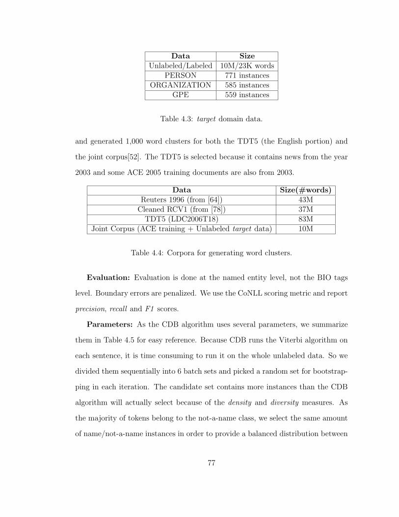
Data SizeUnlabeled/Labeled 10M/23K words

PERSON 771 instancesORGANIZATION 585 instances

GPE 559 instances

Table 4.3: target domain data.

and generated 1,000 word clusters for both the TDT5 (the English portion) and

the joint corpus[52]. The TDT5 is selected because it contains news from the year

2003 and some ACE 2005 training documents are also from 2003.

Data Size(#words)Reuters 1996 (from [64]) 43MCleaned RCV1 (from [78]) 37MTDT5 (LDC2006T18) 83M

Joint Corpus (ACE training + Unlabeled target data) 10M

Table 4.4: Corpora for generating word clusters.

Evaluation: Evaluation is done at the named entity level, not the BIO tags

level. Boundary errors are penalized. We use the CoNLL scoring metric and report

precision, recall and F1 scores.

Parameters: As the CDB algorithm uses several parameters, we summarize

them in Table 4.5 for easy reference. Because CDB runs the Viterbi algorithm on

each sentence, it is time consuming to run it on the whole unlabeled data. So we

divided them sequentially into 6 batch sets and picked a random set for bootstrap-

ping in each iteration. The candidate set contains more instances than the CDB

algorithm will actually select because of the density and diversity measures. As

the majority of tokens belong to the not-a-name class, we select the same amount

of name/not-a-name instances in order to provide a balanced distribution between

77

the name and the not-a-name classes. We tried many different parameter values

and those in Table 4.5 were selected by eyeballing the quality of selected instances.

Parameter Size or ValueBatch Set 60K sentences (roughly 1.7M tokens)

Candidate Set 2000/2000 name/not-a-name instancesDL

T 300/300 name/not-a-name instancesIterations 30diff(i, j) 0.001

Table 4.5: Parameters for CDB.

4.5.2 Performance of the source Domain Model

We build two source models using the ACE 2005 training data in Table 4.2.

The first model is an HMM model with the BILOU states encoding. The second

model is the MEMM model with the BIO encoding using the conventional features

as described in Section 4.4.2 (no word cluster features). Their performances on

both the source and the target domains are summarized in Table 4.6.

Model P R F1 DomainHMM(BILOU) 82.49 81.16 81.82 sourceHMM(BILOU) 53.29 57.52 55.33 targetMEMM(BIO) 84.68 81.54 83.08 sourceMEMM(BIO) 70.02 61.86 65.69 target

Table 4.6: Performance of source models over the 3 name types.

Table 4.6 shows that although both models achieve F1 of 80s on the source

domain, they generalize poorly on the target domain. Comparing the HMM model

with the MEMM model, it seems that the feature based model generalizes better

to the target domain than the generative HMM model even though we did use

78

the word type features as a back-off model similar to [5]. We did not observe the

advantage of using the BILOU scheme as reported in [65] for both the source and

the target domains. Although we could not determine the exact reason why this

happens for the source domain, for the target domain, it contains long translit-

erated Arabic names implying that the state transition from “I” to “I” is more

common in the target than the source domain. This type of transition might not

be observed enough and estimated sufficiently by the fine grained BILOU scheme.

4.5.3 Performance of the Generalized Model

We augmented the source model with word clusters (as described in Section

4.4.2) from the four unlabeled corpora in Table 4.4. Their performance on the

target domain is shown in Table 4.7.

Word clusters P R F1No Cluster 70.02 61.86 65.69Reuters 1996 69.26 64.26 66.67

RCV1 66.33 64.42 65.36TDT5 70.76 66.51 68.57

Joint Corpus 72.82 66.61 69.58

Table 4.7: Performance of the generalized source model.

Table 4.7 shows the superiority of using a joint corpus to generate word clus-

ters: the 10M words joint corpus outperformed the other 3 larger corpora. The

TDT5 corpus is more than 8 times larger than the joint corpus, but is still 1

point behind. Using word clusters from the Reuters corpora (Reuters 1996 and

RCV1) have shown to improve NER systems’ performance on the CoNLL 2003

NER task[65][80]. But they provided limited performance gain for our model

when testing on the target domain. The results shown here indicate the necessity

79

of using a joint corpus or ideally a general purpose corpus for generalizing the

source domain model for cross-domain NER.

4.5.4 Performance of CDB

We start with the generalized source/seed model and run the CDB algorithm

on the unlabeled target domain corpus using the parameters specified in Table

4.5. As mentioned earlier, the seed model is generalized sequentially, that is, word

cluster features are used during each round. We plot F1 score against iteration

in Figure 4.2. The results are obtained by testing the updated model during each

round on the labeled target domain data. The results are averaged on 10 runs.

There are several clear trends in Figure 4.2. First, without using the nov-

elty measure (the line at the bottom), CDB performs worse than generalized seed

model (GSM). Although the seed model is already generalized with word clus-

ters, the most confidently labeled instances might still be more similar to the

source than the target domain. This indicates that novelty is a necessary measure

for cross-domain NER. Comparing the two confidence measures: ComConf and

LocalConf , in general, ComConf outperforms LocalConf . After using the nov-

elty measure, all instances are new to our seed model. So there is some degree of

uncertainty when the model tries to make a local prediction. Not only considering

the local prediction, but also considering how the same token is labeled globally,

the ComConf measure seems to be a better choice in a cross-domain setting.

Regarding the density and the diversity measures, both of them further improve

the performance. Density, however, does not perform well in the first 6 iterations.

We checked the instances that had been selected during these iterations and found

that many of them appear with very strong context words such as Mr., President,

80

Iteration

0 5 10 15 20 25 30 35

F1

68

69

70

71

72

73

74

+ Novelty + Com Conf + Diversity+ Novelty + Com Conf + Density + Novelty + Com Conf + Novelty + LocalConf GSM- Novelty + LocalConf

Figure 4.2: Performance of CDB. GSM stands for generalized seed model at iter-ation 0; + means with and - means without.

General and said. They are considered representative instances according to our

density measure. They can be regarded as cross-domain contexts which might

have been learned by the generalized and un-generalized source domain models. In

contrast, the diversity measure not only considers how representative an instance is

but also prefers a certain degree of difference among the selected instances. Hence,

the diversity measure has achieved the best result CDB could get so far.

The best F score with the diversity measure is 72.85, a 7.16 improvement

compared to the source model. The F score at the last iteration is 72.45, a 6.76

improvement compared to the source model.

81

We also run a standard bootstrapping procedure with the un-generalized seed

model and with the same parameters used for the CDB procedure. The perfor-

mance trends of using different instance selection criteria are similar to those of the

CDB algorithm. The best F score, 70.12, is also obtained with the diversity mea-

sure. This further confirms that the multiple criteria proposed in this paper are

better than a single criterion. CDB with generalized seed model outperformed the

standard bootstrapping by more than 2 points which further indicates the useful-

ness of the combination of feature generalization and multi-criteria-based instance

selection methods proposed in this paper.

4.6 Conclusion

We have described a general cross-domain bootstrapping algorithm for adapting

a model trained only on a source domain to a target domain. We have improved

the source model’s F score by around 7 points. This is achieved without using

any annotated data from the target domain and without explicitly encoding any

target-domain-specific knowledge into our system. The improvement is largely

due to the incorporation of the global evidence in feature generalization and the

multi-criteria-based instance selection method.

Our immediate future work is to find a natural stopping criterion for the

bootstrapping procedure, perhaps through the detection of semantic drift [57][75].

Gazetteer resources have proven to be a powerful knowledge base for improving

NER performance[22]. The only gazetteer in CDB now is a country and US state

list. So another promising research avenue is to study how to automatically learn

or mine a target domain named entity dictionary to further improve our system’s

82

performance.

83

Chapter 5

Conclusion and Future Work

5.1 Conclusion

Recent advances in information extraction move beyond narrowly restricted

domains and shift the focus to a variety of new emerging domains. These include

terrorism reports, scientific publications, legal and medical documents, microblog

texts such as tweets and Foursquare tips, collaboratively generated web documents

such as Wikipedia, and many more. This however, brings a great many new tasks

and challenges, and it is not desirable to hire human experts to annotate data for

every new task of every new domain.

This dissertation moves a step further to solve these emerging problems with

low cost and in a fast and accurate way. Specifically, we have presented three

systems: the relation type extension system based on active learning (Chapter

2), the relation type extension system based on semi-supervised learning (Chapter

3), and the cross-domain bootstrapping system for domain adaptive named entity

extraction (Chapter 4).

84

The main contribution of this dissertation is its exploration of using both local

and global evidence for fast system development. The benefits of using these two

types of evidence are substantial: the co-testing procedure based on the local and

global views of relation instances reduced annotation cost by 97% while maintain-

ing the performance level of supervised learning. The use of pattern clusters as

the global view in semi-supervised relation pattern acquisition not only greatly im-

proved the quality of learned patterns but also contributed to a natural stopping

criterion. The generalization of local lexical features using word clusters and the

instance selection based on global evidence in the cross-domain bootstrapping pro-

cedure were able to improve the source model’s performance on the target domain

by 7% F1 without annotating any target domain data.

5.2 Future Work

Active Learning for Relation Type Extension. For investigating the

feasibility of the proposed active learning approach, this dissertation performed

simulated active learning experiments with the ACE 2004 annotated corpora. This

simplifies the evaluation of active learning from many factors that might arise in

real world active learning settings: the effect of downstream component errors such

as name and entity extraction, the effect of annotation consistency by one or more

annotators, the time of model re-training in each iteration, etc. We are excited to

explore these factors in our future real world active learning experiments.

Another direction of this branch of research, as mentioned in the last section of

Chapter 2, is to combine semi-supervised learning with active learning to further

reduce annotation cost.

85

Semi-supervised Learning for Relation Type Extension. Currently the

seed patterns used are defined manually, which is far from being a desirable and

principled way. A promising research avenue is to study the automatic discovery

and selection of seed patterns. More specifically, we will focus on how to conduct

seed discovery and selection based on the global evidence, i.e., pattern clusters. A

two-stage procedure might move this idea forward: manually define some initial

seed patterns and then choose the good ones from the target cluster as the actual

seeds.

Cross-domain Bootstrapping for Named Entity Recognition. In do-

main adaptation for named entity recognition, one may have a dictionary of names

for the target domain but no labeled target domain data. This represents a more

and more realistic scenario because of the emergence of collaboratively generated

knowledge bases such as Wikipedia. There are two future directions for our cross-

domain bootstrapping to accommodate this scenario: 1) extracting dictionary-

based features to further generalize features; 2) combining with distantly annotated

data (by aligning a dictionary with texts to generate training data) to further im-

prove performance.

Other Future Research Avenues. As the ultimate goal of information

extraction is to power other applications, I see the opportunity to expand the scope

of my research to contribute to other fields of study. For example, the information

retrieval community shows great interest in entity-oriented search such as people

search, job search and product search. Extracting the entities and the attributes

of them (similar to relation extraction) with high performance is a first and crucial

step for finding relevant documents for the entities. It would be exciting to bridge

the gap between disciplines.

86

Bibliography

[1] Steven Abney. Semisupervised Learning for Computational Linguistics. Chap-

man and Hall. 2008.

[2] Eugene Agichtein and Luis Gravano. Snowball: Extracting relations from large

plain-text collections. In Proc. of the Fifth ACM International Conference on

Digital Libraries. 2000.

[3] Rie K. Ando and Tong Zhang. A Framework for Learning Predictive Struc-

tures from Multiple Tasks and Unlabeled Data. Journal of Machine Learning

Research, Vol 6:1817-1853. 2005.

[4] Markus Becker, Ben Hachey, Beatrice Alex, and Claire Grover. Optimising

Selective Sampling for Bootstrapping Named Entity Recognition. Proceedings

of the ICML-2005 Workshop on Learning with Multiple Views. 2005.

[5] Daniel M. Bikel, Scott Miller, Richard Schwartz and Ralph Weischedel.

Nymble: a high performance learning name-finder. In Proc. of ANLP. 1997.

[6] John Blitzer, Ryan McDonald, and Fernando Pereira. Domain adaptation with

structural correspondence learning. In Proc. of EMNLP. 2006.

87

[7] Avrim Blum and Tom Mitchell. Combining la-beled and unlabeled data with

co-training. In Pro-ceedings of the Eleventh Annual Conference on Computa-

tional Learning Theory. 1998.

[8] Andrew Borthwick. A Maximum Entropy Approach to Named Entity Recog-

nition. Ph.D. thesis, New York University. 1999.

[9] Andrew Borthwick, John Sterling, Eugene Agichtein and Ralph Grishman.

Exploiting Diverse Knowledge Sources via Maximum Entropy in Named Entity

Recognition. In Proc. of Sixth WVLC. 1998.

[10] Elizabeth Boschee, Ralph Weischedel, and Alex Zamanian. Automatic infor-

mation extraction. In Proceedings of the International Conference on Intelli-

gence Analysis. 2005.

[11] Sergey Brin. Extracting patterns and relations from the World-Wide Web. In

Proc. of the 1998 Intl. Workshop on the Web and Databases. 1998.

[12] Peter F. Brown, Vincent J. Della Pietra, Peter V. deSouza, Jenifer C. Lai,

and Robert L. Mercer. Class-based n-gram models of natural language. Com-

putational Linguistics, 18(4):467-479. 1992.

[13] Razvan C. Bunescu and Raymond J. Mooney. A shortest path dependency

kenrel for relation extraction. In Proceedings of HLT/EMNLP. 2005.

[14] Razvan C. Bunescu and Raymond J. Mooney. Subsequence kernels for relation

extraction. In Proceedings of NIPS. 2005.

88

[15] Andrew Carlson, Justin Betteridge, Richard C. Wang, Estevam Rafael Hr-

uschka Junior and Tom M. Mitchell.Coupled Semi-Supervised Learning for

Information Extraction. In WSDM. 2010.

[16] Yee Seng Chan and Dan Roth. Exploiting background knowledge for relation

extraction. In Proc. of COLING. 2010.

[17] Ming-Wei Chang, Lev Ratinov, and Dan Roth. Guiding semisupervision with

constraint-driven learning. In Proc. of ACL-2007, Prague. 2007.

[18] Ciprian Chelba and Alex Acero. Adaptation of maximum entropy capitalizer:

Little data can help a lot. In Proc. of EMNLP, pages 285-292. 2004.

[19] Zheng Chen and Heng Ji. Can One Language Bootstrap the Other: A Case

Study on Event Extraction. In NAACL HLT Workshop on Semi-supervised

Learning for NLP. 2009.

[20] Hai Leong Chieu and Hwee Tou Ng. Named entity recognition with a maximum

entropy approach. In Proceedings of CoNLL-2003. 2003.

[21] Massimiliano Ciaramita and Yasemin Altun. Named-entity recognition in

novel domains with external lexical knowledge. In Advances in Structured

Learning for Text and Speech Processing Workshop. 2005.

[22] William W. Cohen and Sunita Sarawagi. Exploiting Dictionaries in Named

Entity Extraction: Combining SemiMarkov Extraction Processes and Data

Integration Methods. In Proc. of KDD. 2004.

[23] Michael Collins and Yoram Singer. Unsupervised Models for Named Entity

Classification. In Proc. of EMNLP-99. 1999.

89

[24] James R. Curran, Tara Murphy, and Bernhard Scholz. Minimising semantic

drift with Mutual Exclusion Bootstrapping. In Proc. of PACLING. 2007.

[25] Hal Daum III. Frustratingly easy domain adaptation. In Proc. of ACL. 2007.

[26] Hal Daum III and Daniel Marcu. Domain adaptation for statistical classifiers.

Journal of Artificial Intelligence Research, 26:101-126. 2006.

[27] Mark Dredze, John Blitzer, Partha Talukdar, Kuzman Ganchev, Joao Graca,

and Fernando Pereira. Frustratingly Hard Domain Adaptation for Parsing. In

Proc. of CoNLL. 2007.

[28] Jenny Rose Finkel and Christopher D. Manning. Hierarchical bayesian domain

adaptation. In Proc. of NAACL. 2009.

[29] Jenny Rose Finkel, Trond Grenager, and Christopher Manning. Incorporating

non-local information into information extraction systems by gibbs sampling.

In Proc. of ACL. 2005.

[30] Radu Florian, Abe Ittycheriah, Hongyan Jing, and Tong Zhang. Named en-

tity recognition through classifier combination. In Proceedings of CoNLL-2003.

2003.

[31] R. Florian, H. Hassan, A. Ittycheriah, H. Jing, N. Kambhatla, X. Luo, N.

Nicolov, and S. Roukos. A statistical model for multilingual entity detection

and tracking. In Proc. of HLT-NAACL. 2004.

[32] Radu Florian, John Pitrelli, Salim Roukos, Imed Zitouni. Improving Mention

Detection Robustness to Noisy Input. In Proc. of ENMLP. 2010.

90

[33] Ralph Grishman. Information Extraction: Capabilities and Challenges. Notes

prepared for the 2012 International Winter School in Language and Speech

Technologies. 2012.

[34] R. Grishman and B. Sundheim. Message Understanding Conference-6: A

Brief History. In Proceedings of the COLING, 1996.

[35] Ralph Grishman, David Westbrook and Adam Meyers. NYUs English ACE

2005 System Description. ACE 2005 Evaluation Workshop. 2005.

[36] Zellig S. Harris. Distributional Structure. Word. Vol 10,1954, 146-162. 1954.

[37] Takaaki Hasegawa, Satoshi Sekine, Ralph Grishman. Discovering Relations

among Named Entities from Large Corpora. In Proc. of ACL-04. 2004.

[38] Marti Hearst. Automatic acquisition of hyponyms from large text corpora. In

Proc. of the 14th Intl. Conf. on Computational Linguistics. 1992.

[39] Ruihong Huang and Ellen Riloff. Inducing Domain-specific Semantic Class

Taggers from (Almost) Nothing. In Proc. of ACL. 2010.

[40] Earl B. Hunt, Philip J. Stone and Janet Marin. Experiments in Induction.

New York: Academic Press. 1966.

[41] Heng Ji and Ralph Grishman. Data Selection in Semi-supervised Learning for

Name Tagging. In ACL 2006 Workshop on Information Extraction Beyond

the Document. 2006.

[42] Heng Ji, Ralph Grishman and Hoa Trang Dang. 2011. An Overview of the

TAC2011 Knowledge Base Population Track. Proc. Text Analysis Conference

(TAC2011). 2011.

91

[43] Jing Jiang. Multi-task transfer learning for weak-ly-supervised relation extrac-

tion. In Proceedings of ACL-IJCNLP-09. 2009.

[44] Jing Jiang and ChengXiang Zhai. Exploiting domain structure for named en-

tity recognition. In Proceedings of HLT-NAACL’06. 2006.

[45] Jing Jiang and ChengXiang Zhai. A systematic exploration of the feature space

for relation extrac-tion. In Proceedings of HLT-NAACL-07. 2007.

[46] Jing Jiang and ChengXiang Zhai. Instance weighting for domain adaptation

in nlp. In Proceedings of ACL. 2007.

[47] Rosie Jones, Rayid Ghani, Tom Mitchell, Ellen Riloff. Active learning for in-

formation extraction with multiple view feature sets. In ECML 2003 Workshop

on Adaptive Text Extraction and Mining. 2003.

[48] Nanda Kambhatla. Combining lexical, syntactic, and semantic features with

maximum entropy models for information extraction. In Proceedings of ACL-

04. 2004.

[49] Terry Koo, Xavier Carreras, and Michael Collins. Simple Semi-supervised De-

pendency Parsing. In Proceedings of ACL-08: HLT. 2008.

[50] Zornista Kozareva and Eduard Hovy. Not all seeds are equal: Measuring the

quality of text mining seeds. In NAACL-10. 2010.

[51] Vijay Krishnan and Christopher D. Manning. An effective two stage model

for exploiting non-local dependencies in named entity recognition. In Proc. of

ACL. 2006.

92

[52] Percy Liang. Semi-Supervised Learning for Natural Language. Masters thesis,

Massachusetts Institute of Technology. 2005.

[53] Dekang Lin and Patrick Pantel. Discovery of inference rules for question-

answering. Natural Language Engineering, 7(4):343-360. 2001.

[54] Dekang Lin and Xiaoyun Wu. Phrase Clustering for Discriminative Learning.

In Proceedings of the ACL and IJCNLP 2009. 2009.

[55] Marie-Catherine de Marneffe and Christopher D. Manning. The Stanford typed

dependencies representation. In COLING Workshop on Cross-framework and

Cross-domain Parser Evaluation. 2008.

[56] Andrew McCallum, Dayne Freitag and Fernando Pereira. Maximum Entropy

Markov Models for Information Extraction and Segmentation. In Proc. of

ICML. 2000.

[57] Tara McIntosh. Unsupervised discovery of negative categories in lexicon boot-

strapping. In Proc of EMNLP. 2010.

[58] Scott Miller, Heidi Fox, Lance Ramshaw, and Ralph Weischedel. A novel use

of statistical parsing to extract information from text. In Proc. of NAACL.

2000.

[59] Scott Miller, Jethran Guinness and Alex Zamanian. Name Tagging with Word

Clusters and Discriminative Training. In Proc. of HLT-NAACL. 2004.

[60] Ion Muslea, Steve Minton, and Craig Knoblock. Selective sampling with redun-

dant views. In Pro-ceedings of the Fifteenth National Conference on Artificial

Intelligence. 2000.

93

[61] David Nadeau and Satoshi Sekine. A Survey of Named Entity Recognition and

Classification. In: Sekine, S. and Ranchhod, E. Named Entities: Recognition,

classification and use. Special issue of Lingvisticae Investigationes. 30(1) pp.

3-26. 2007.

[62] Patrick Pantel and Marco Pennacchiotti. Espresso: Leveraging Generic Pat-

terns for Automatically Harvesting Semantic Relations. In Proc. of COLING-

06 and ACL-06. 2006.

[63] Longhua Qian, Guodong Zhou, Qiaoming Zhu and Peide Qian. Exploiting

constituent dependencies for tree kernel-based semantic relation extraction. In

Proc. of COLING. 2008.

[64] John Ross Quinlan. Induction of decision trees. Machine Learning, 1(1), 81-

106. 1986.

[65] Lev Ratinov and Dan Roth. Design challenges and misconceptions in named

entity recognition. In Proceedings of CoNLL-09. 2009.

[66] Deepak Ravichandran and Eduard Hovy. Learning Surface Text Patterns for

a Question Answering System. In Proc. of ACL-2002. 2002.

[67] E. Riloff and R. Jones. Learning Dictionaries for Information Extraction by

Multi-Level Bootstrapping. In Proceedings of AAAI-99. 1999.

[68] Brian Roark and Michiel Bacchiani. Supervised and unsupervised PCFG adap-

tation to novel domains. In Proc. of HLT-NAACL, pages 126-133. 2003.

[69] Benjamin Rosenfeld, Ronen Feldman. Clustering for Unsupervised Relation

Identification. In Proc. of CIKM 07. 2007.

94

[70] Satoshi Sekine. A Linguistic Knowledge Discovery Tool: Very Large Ngram

Database Search with Arbitrary Wildcards. In proceedings of the 22nd Interna-

tional Conference on Computational Linguistics, Manchester, England. 2008.

[71] Dan Shen, Jie Zhang, Jian Su, Guodong Zhou, and Chew-Lim Tan. Multi-

criteria-based active learning for named entity recognition. In Proceedings of

ACL. 2004.

[72] Mark Stevenson and Mark A. Greenwood. A Semantic Approach to IE Pattern

Induction. In Proc. of the 43rd Annual Meeting of the ACL. 2005.

[73] Mark Stevenson and Mark A. Greenwood. Comparing Information Extraction

Pattern Models. In Proceedings of the Workshop on Information Extraction

Beyond The Document. 2006.

[74] Ang Sun. A Two-stage Bootstrapping Algorithm for Relation Extraction. In

RANLP-09. 2009.

[75] Ang Sun and Ralph Grishman. Semi-supervised Semantic Pattern Discovery

with Guidance from Un-supervised Pattern Clusters. In Proc. of COLING-10.

2010.

[76] Ang Sun and Ralph Grishman. Semi-supervised Relation Extraction with

Large-scale Word Clustering. In Proc. of ACL-11. 2011.

[77] Ang Sun, Ralph Grishman. Cross-Domain Bootstrapping for Named Entity

Recognition. In proc. of SIGIR 2011 Workshop on Entity-Oriented Search.

2011.

95

[78] Ang Sun, Ralph Grishman, Wei Xu and Bonan Min. New York University

2011 System for KBP Slot Filling. In proceedings of TAC. 2011.

[79] Erik Tjong and Fien De Meulder. Introduction to the conll-2003 shared task:

Language independent named entity recognition. In Proceedings of Conference

on Computational Natural Language Learning. 2003.

[80] Joseph Turian, Lev-Arie Ratinov, and Yoshua Bengio. Word representations:

A simple and general method for semi-supervised learning. In Proceedings of

ACL. 2010.

[81] Vishnu Vyas, Patrick Pantel and Eric Crestan. Helping Editors Choose Better

Seed Sets for Entity Expansion. In Proceedings of CIKM-09. 2009.

[82] Yingchuan Wong and Hwee Tou Ng. One Class per Named Entity: Exploiting

Unlabeled Text for Named Entity Recognition. In Proc. of IJCAI-07. 2007.

[83] Dan Wu, Wee Sun Lee, Nan Ye, and Hai Leong Chieu. Domain adaptive

bootstrapping for named entity recognition. In Proc. of EMNLP. 2010.

[84] Roman Yangarber. Counter-training in the discovery of semantic patterns. In

Proc. of ACL. 2003.

[85] Roman Yangarber, Ralph Grishman, Pasi Tapanainen and Silja Huttunen.

Automatic acquisition of domain knowledge for information extraction. In

Proc. of COLING. 2000.

[86] Roman Yangarber, Winston Lin and Ralph Grishman. Unsupervised Learning

of Generalized Names. In Proc. of COLING. 2002.

96

[87] David Yarowsky. Unsupervised word sense disambiguation rivaling supervised

methods. In Proc. of ACL-95. 1995.

[88] Dmitry Zelenko, Chinatsu Aone, and Anthony Richardella. Kernel methods

for relation extraction. Journal of Machine Learning Research, 3:1083-1106.

2003.

[89] Zhu Zhang. Weakly supervised relation classification for information extrac-

tion. In Proc. of CIKM2004. 2004.

[90] Min Zhang, Jian Su, Danmei Wang, Guodong Zhou, and Chew Lim Tan. Dis-

covering Relations Between Named Entities from a Large Raw Corpus Using

Tree Similarity-Based Clustering. In IJCNLP 2005, LNAI 3651, pp. 378-389.

2005.

[91] Min Zhang, Jie Zhang, Jian Su, and GuoDong Zhou. A composite kernel

to extract relations between entities with both flat and structured features. In

Proceedings of COLING-ACL-06. 2006.

[92] Shubin Zhao and Ralph Grishman. Extracting relations with integrated infor-

mation using kernel methods. In Proceedings of ACL. 2005.

[93] Guodong Zhou, Jian Su, Jie Zhang, and Min Zhang. Exploring various knowl-

edge in relation extraction. In Proceedings of ACL-05. 2005.

[94] GuoDong Zhou, JunHui Li, LongHua Qian and QiaoMing Zhu. Semi-

supervised learning for relation extraction. IJCNLP2008:32-39. 2008.

97

[95] Guodong Zhou, Min Zhang, DongHong Ji, and QiaoMing Zhu. Tree kernel-

based relation extraction with context-sensitive structured parse tree informa-

tion. In Proceedings of EMNLP-CoNLL-07. 2007.

98