1

Rapid falling of an orbiting moon to its parent planet due

to tidal-seismic resonance

Yuan Tian1, Yingcai Zheng1 1Department of Earth and Atmospheric Sciences, University of Houston, Houston, TX

2

Abstract

Tidal force plays an important role in the evolution of the planet-moon system. The tidal

force of a moon can excite seismic waves in the planet it is orbiting. A tidal-seismic resonance is

expected when a tidal force frequency matches a free-oscillation frequency of the planet. Here

we show that when the moon is close to the planet, the tidal-seismic resonance can cause

large-amplitude seismic waves, which can change the shape of the planet and in turn exert a

negative torque on the moon to cause it to fall rapidly toward the planet. We postulate that the

tidal-seismic resonance may be an important mechanism which can accelerate planet accretion

process. On the other hand, tidal-seismic resonance effect can also be used to interrogate

planet interior by long term tracking of the orbital change of the moon.

Keywords: Resonance, tidal force, normal mode, orbital evolution

3

1. Introduction

Darwin (1898) first proposed the idea of a gravity-seismic coupled resonance of a fluid

planet to explain the Moon formation and he argued that the violent vibration of the planet at

resonance “… shook the planet to pieces, detaching huge fragments which ultimately were

consolidated into the Moon?”. While Darwin’s idea of moon formation theory had been largely

discarded, very little work has been done to investigate possible consequences of the tidal-

seismic resonance for a planet-moon system, in particular for a solid planet.

Tidal force frequencies are usually out of the range of planet free oscillation (or normal

mode) frequencies. Even the tidal force of the fastest rotating system in solar system (i.e.,

Mars-Phobos system) does not have significant effect on the martian free oscillation in the

current orbital configuration (Lognonné et al., 2000).

However, in some cases can tidal force frequencies intrude into the frequency range of

the planet normal modes. For example, the tidal force on a rapid rotating planet can excite

normal modes of the planet (Braviner and Ogilvie, 2014a, b; Barker et al., 2016). Interaction

between Saturn ring and Saturn can excite acoustic free oscillation of Saturn (Marley, 1991;

Marley and Porco, 1993; Marley, 2014). Fuller (2014) used the tidal force to detect the acoustic

free oscillation frequencies from observing density wave in the Saturn ring.

Our goal here is to do a theoretical and numerical analysis to investigate some first

order effects of the tidal-seismic resonance.

2. Material and Methods

2.1. Model setup

4

In our analysis, we make some simplifications and approximations. We consider a planet-

moon system as a binary rotating system in an inertial reference frame. We assume the moon

as a point mass and we do not consider potential fragmentation of the moon at the Roche limit

(Aggarwal and Oberbeck, 1974; Asphaug and Benz, 1994; Black and Mittal, 2015). The planet

does not spin with respect to the reference frame. We assume that the moon’s orbit is circular

on the planet’s equatorial plane. The orbiting period of the moon can be computed using the

Kepler’s law. We compute the moon’s tidal force for every point in the planet by subtracting

the centrifugal force from the gravitational attraction force.

We consider two planet models, model-1 which has no topography and model-2 with

topography. In model-1, the planet is a homogeneous elastic spherical solid with no

topography. We set the compressional wave velocity in the solid as 𝑣" = 3 km/s and shear

wave velocity 𝑣% = 1.2 km/s. We set the radius of the planet as 2000 km. We use the mass-

radius relation (Chen and Kipping, 2017) to set the planet density as 𝜌 = 2.84𝑘𝑔/𝑚1. The mass

of the moon is taken as, 1023 kg (as a reference, this is similar to the mass of an object like

Phobos), which is about 1045 times of the mass the planet. We also consider the effect of Q,

which captures the dissipation effect of the planet. Previous work showed that Q could cause

tidal phase lag and was important in calculating the orbital decay of moon (Zharkov and

Gudkova, 1997; e.g., Bills et al., 2005; Nimmo and Faul, 2013; Zheng et al., 2015). The planet

topography can also play a role in the tidal-seismic resonance. Therefore, we also consider a

second planet of the same material but with a randomly generated topography (named as

model-2).

5

2.2. Method

To see when the resonance can occur, we can compute the planet normal-mode

frequencies (see Appendix-A) and the tidal forces (see Appendix-B). Because the moon orbits

around the planet periodically, the tidal force is periodic for any location in the planet. If the

orbit frequency is designated as , it can also excite higher order harmonics at integer

frequencies such as where n=2, 3, 4, … The tidal-seismic resonance occurs when a tidal

force frequency is the same as a normal-mode frequency (Figure 1). Tidal force preferentially

excites the fundamental spheroidal normal mode, 0Sn, where n is the degree in the surface

spherical harmonic function.

Figure 1. Tidal force and planet normal mode frequencies for model-1. Solid lines are tidal force

frequencies calculated at a location on the planet equator. Vertical dash lines are planet free-

oscillation frequencies for the spheroidal 0Sn normal modes (n=2, 3, 4 …). Tidal-seismic resonance

occurs when tidal force frequencies intersect the planet free oscillation frequencies at red circles.

ω0

nω0

6

The orbiting moon exerts a cyclic tidal force for every point in the planet. Therefore, this

tidal force can cause seismic displacement in the planet to deform the planet figure. The

change of figure of the planet can change the planet gravitational field to exert a net torque on

the moon. To compute this torque, we need to compute the tidal-force induced seismic

wavefield and we use the boundary element integral equation approach (Zheng et al., 2016a) to

do so (see Appendix C). The advantage of this computational method is that it is implemented

in the frequency domain and can model long-term seismic field evolution (i.e., can avoid

numerical dispersion in many time-domain methods) and can also handle planet topography.

We did not include the effect of self-gravitation on the seismic waves (Dahlen and Tromp, 1998)

in our calculation. Once we obtain the seismic wavfield we can compute the time dependent

torque on the moon and the orbital decay rate of the moon (See Appendix D).

3. Results

3.1. Tidal-seismic resonance at low orbits

At low orbits, it is evident that the orbital decay rate overall is increasing as the moon is

approaching the planet and the tidal seismic effect punctuates/accelerates this trend locally at

several distinct orbital radii (“peaks” in Figure 2). These are special orbital radii at which strong

torque has been exerted on the orbiting moon due to the resonance. Because of their specialty,

we call these orbital radii, , where 𝑛 = 1, 2, 3…. At , the planet 0Sn normal mode frequency

is exactly 𝑛 times of the orbital frequency at . In these cases, both the tidal force and the 0Sn

mode have degree-𝑛 spatial patterns in the planet. Therefore, this is a simultaneous coupling

rn* rn

*

rn*

7

between the temporary and spatial frequencies (i.e., degree-𝑛) at , which can cause very

strong excitation of seismic displacements in the planet (Figure 2).

We compute orbital decay rates for several different Q values. Large Q values correspond to large

orbital decay rates because the induced seismic surface displacement and torque are large

(Figure 2). In particular, at 𝑟:∗ where the excited normal mode is the gravest “football-shaped”

mode, the orbital decay rate is on the order of ~1-10 cm/s for different Q values (Figure 2) for

this particular model. The important thing to note is the relative orbit decay rate for this model.

At the tidal-seismic resonance orbit, the orbit decay rate is 2 orders of magnitude more than that

for a neighboring orbit where there is no resonance.

We note that the exact numerical value for orbit decay may vary from model to model.

However, the tidal-seismic resonance can significantly accelerate the orbital decay (“peaks” in

Figure 2 compared to the smooth background trend). The greater the Q value, the sharper the

peaks are. To verify whether these peaks are indeed caused by tidal-seismic resonance, we

analytically calculated the normal mode 0Sn frequencies of the planet (See Appendix A). And

then, we calculate the corresponding 𝑟<∗ whose orbital frequency is 1/n times of the 0Sn

frequency. We found the calculated 𝑟<∗ based on the 0Sn frequency correspond to the peaks of

the moon orbital decay rate (Figure 2). In conclusion, the rapid falling of the moon is caused by

tidal-excited normal modes of the planet. When the moon’s orbit radius is large (e.g., >

m), tidal-seismic resonance effect is not obvious. In this case, smaller Q gives larger

orbital decay rate and this is consistent with the tidal drag due to anelasticity effect (Bills et al.,

2005).

rn*

2.5×106

8

Figure 2. Calculated moon orbital decay rate at different orbital radii and for different Q values

for model-1. The horizontal axis is the orbital radius of the moon. The radius of the planet is

2 × 103m. We also label excited normal modes, , expected to be seen for the tidal-

seismic resonance.

3.2. Topography induced tidal-seismic resonance

At higher orbits, (orbital radius greater than 2.5 × 103𝑚 in this case), resonance can occur

when matches the frequency where both m and n are integers but usually . In

this case, spatial frequencies of the normal mode and the tidal force de-couple.

In principle, a degree-m tidal force field cannot excite degree-n normal mode for a purely

spherical planet (i.e., model-1) because these two fields are orthogonal to each other in space.

However, if the planet is not spherical (i.e., model-2), the tidal-seismic resonance can still exist

0Sn ,n≥2

mω0 0 Sn m > n

9

because topography could couple modes of different degrees. Our purpose here is to

investigate the topography-induced tidal-seismic effect.

Figure 3. A topography model (model 2) for the planet. We have exaggerated the plotting of the

topography by 20 times. Colors indicate topography relative to the mean radius of the planet and

the unit of the size is in meters. The thick red line is the equator. The blue vertical thick line is the

axis through the poles.

For model-2, we randomly generated a topography for the planet and filtered it spatially

using spherical harmonics up to order 6 (including 6) (Figure 3). We use the same numerical

procedure laid out in Section 3.1 to compute the seismic wavefield for model-2 and compute

10

the torque on the moon and then the orbital decay rate of the moon. To see the topography

effect on the tidal seismic resonance, we can take derivative of the orbital decay rate with

respect to the orbital radius and we find localized changes at some radii (Figure 4a). These

changes are actually due to topography induced tidal-seismic resonance. To validate this claim,

we run our wavefield modeling on two models (model-1 and model-2) and obtain histories of

orbital decay rates for both models. We calculate the derivative of the orbital decay rate with

respect to orbital radius for the two models (Figure 4 a &b). We see localized changes for the

topography model, model-2 (Figure 4a). In contrast, we see a smooth curve of orbital decay

rate derivative on model-1 without topography (Figure 4b). Hence, topography can induce tidal-

seismic resonance at higher orbits.

11

Figure 4. Derivative of the orbital decay rate with respect to orbit radius. (a) for model-2 with

topography; (b) for model-1 without topography. Here, f@ is the frequency of the normal mode

. A dashed line shows the orbit whose orbital frequency is , (n and m are integers)

labeled next the dashed line.

4. Discussions

As we know, tidal force plays an important role on the orbital evolution of Mars moon, Phobos

(Black and Mittal, 2015; Hesselbrock and Minton, 2017). Due to tidal torque, Phobos is spiraling

towards Mars. Will the tidal-seismic resonance play a role in this system? At present time,

Phobos is too far from inducing a significant tidal-seismic resonance. However, when Phobos’

orbit decays to about 1.97 (current orbit is about 2.77) times of the martian radius, topography

induced tidal-seismic resonance will be able to cause an orbit decay, estimated about

1042A𝑚/𝑠 based on current martian topography and an approximate homogenous Mars model

(P-wave velocity 𝑣" = 7.4𝑘𝑚/𝑠 , S-wave velocity 𝑣% = 3.6𝑘𝑚/𝑠, density 𝜌 = 4000𝑘𝑔/𝑚1to

match a 0S2 period of about 2300 s (Zheng et al., 2015)). This rate is then comparable to the

current orbital decay rate of Phobos, which is about 1.28 × 104F𝑚/𝑠 (Bills et al., 2005). As

Phobos keeps falling towards Mars, the effect of tidal-seismic resonance will be more and more

influential to pull Phobos to Mars. Because of the tidal-seismic resonance, we note that Phobos

cannot stay at low orbits for long time even it passes the Roche limit and is not fragmented by

Mars tidal force.

5. Conclusions

0Sn fn / m

12

Tidal-seismic resonance effect can be important in understanding planet-moon evolution. The

tidal seismic resonance can result in a large negative torque, which can increase the orbital

decay rate of the moon toward the planet it is orbiting by one order of magnitude. It can also

significantly accelerate the accretion process. The tidal-seismic phenomenon may also provide

us a potential possible way to interrogate structure and composition information of a planet

without having to land an instrument on the surface of planet. By precisely measuring the

orbital decay rate as a function of radii, we can then infer the normal modes frequencies of the

planet, which can tell a wealth of information about the planet interior.

Declarations of interest: none

References

Aggarwal, H.R., Oberbeck, V.R., 1974. ROCHE LIMIT OF A SOLID BODY. Astrophys. J. 191, 577-588.

Aki, K., Richards, P.G., 2002. Quantitative seismology.

Asphaug, E., Benz, W., 1994. Density of Comet Shoemaker-Levy-9 Deduced by Modeling Breakup of the Parent Rubble-Pile. Nature 370, 120-124.

Barker, A.J., Braviner, H.J., Ogilvie, G.I., 2016. Non-linear tides in a homogeneous rotating planet or star: global modes and elliptical instability. Monthly Notices of the Royal Astronomical Society 459, 924-938.

Ben-Menahem, A., Singh, S.J., 1981. Seismic waves and sources. Springer-Verlag New York Inc.

Bills, B.G., Neumann, G.A., Smith, D.E., Zuber, M.T., 2005. Improved estimate of tidal dissipation within Mars from MOLA observations of the shadow of Phobos. Journal of Geophysical Research-Planets 110.

Black, B.A., Mittal, T., 2015. The demise of Phobos and development of a Martian ring system. Nature Geoscience 8, 913-U936.

13

Braviner, H.J., Ogilvie, G.I., 2014a. Tidal interactions of a Maclaurin spheroid–I. Properties of free oscillation modes. Monthly Notices of the Royal Astronomical Society 441, 2321-2345.

Braviner, H.J., Ogilvie, G.I., 2014b. Tidal interactions of a Maclaurin spheroid–II. Resonant excitation of modes by a close, misaligned orbit. Monthly Notices of the Royal Astronomical Society 447, 1141-1153.

Chen, J.J., Kipping, D., 2017. PROBABILISTIC FORECASTING OF THE MASSES AND RADII OF OTHER WORLDS. Astrophys. J. 834.

Dahlen, F.A., Tromp, J., 1998. Theoretical Global Seismology. Princeton University Press, Princeton, New Jersey.

Darwin, G.H., 1898. The evolution of satellites. The Atlantic Monthly 81, 444-455.

Fuller, J., 2014. Saturn ring seismology: Evidence for stable stratification in the deep interior of Saturn. Icarus 242, 283-296.

Hesselbrock, A.J., Minton, D.A., 2017. An ongoing satellite–ring cycle of Mars and the origins of Phobos and Deimos. Nature Geoscience 10, 266.

Lognonné, P., Giardini, D., Banerdt, B., Gagnepain-Beyneix, J., Mocquet, A., Spohn, T., Karczewski, J., Schibler, P., Cacho, S., Pike, W., 2000. The NetLander very broad band seismometer. Planetary and Space Science 48, 1289-1302.

Marley, M.S., 1991. Nonradial oscillations of Saturn. Icarus 94, 420-435.

Marley, M.S., 2014. Saturn ring seismology: Looking beyond first order resonances. Icarus 234, 194-199.

Marley, M.S., Porco, C.C., 1993. Planetary acoustic mode seismology: Saturn's rings. Icarus 106, 508-524.

Nimmo, F., Faul, U.H., 2013. Dissipation at tidal and seismic frequencies in a melt-free, anhydrous Mars. Journal of Geophysical Research-Planets 118, 2558-2569.

Taylor, P.A., Margot, J.L., 2010. Tidal evolution of close binary asteroid systems. Celestial Mechanics & Dynamical Astronomy 108, 315-338.

Zharkov, V., Gudkova, T., 1997. On the dissipative factor of the Martian interiors. Planetary and space science 45, 401-407.

Zheng, Y., Malallah, A.H., Fehler, M.C., Hu, H., 2016a. 2D full-waveform modeling of seismic waves in layered karstic media. Geophysics 81, T25-T34.

Zheng, Y., Malallah, A.H., Fehler, M.C., Hu, H., 2016b. 2D full-waveform modeling of seismic waves in layered karstic media. Geophysics 81, T25.

14

Zheng, Y., Nimmo, F., Lay, T., 2015. Seismological implications of a lithospheric low seismic velocity zone in Mars. Physics of the Earth and Planetary Interiors 240, 132-141.

15

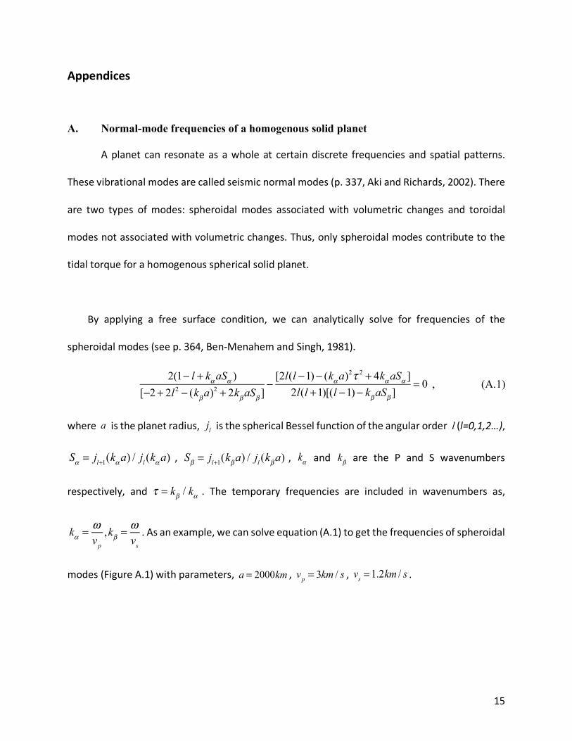
Appendices

A. Normal-mode frequencies of a homogenous solid planet

A planet can resonate as a whole at certain discrete frequencies and spatial patterns.

These vibrational modes are called seismic normal modes (p. 337, Aki and Richards, 2002). There

are two types of modes: spheroidal modes associated with volumetric changes and toroidal

modes not associated with volumetric changes. Thus, only spheroidal modes contribute to the

tidal torque for a homogenous spherical solid planet.

By applying a free surface condition, we can analytically solve for frequencies of the

spheroidal modes (see p. 364, Ben-Menahem and Singh, 1981).

, (A.1)

where is the planet radius, is the spherical Bessel function of the angular order (l=0,1,2…),

, , and are the P and S wavenumbers

respectively, and . The temporary frequencies are included in wavenumbers as,

. As an example, we can solve equation (A.1) to get the frequencies of spheroidal

modes (Figure A.1) with parameters, , , .

2(1− l + kαaSα )[−2+ 2l2 − (kβa)

2 + 2kβaSβ ]−[2l(l −1)− (kαa)

2τ 2 + 4kαaSα ]2l(l +1)[(l −1)− kβaSβ ]

= 0

a jl l

Sα = jl+1(kαa) / jl (kαa) Sβ = jl+1(kβa) / jl (kβa) kα kβ

τ = kβ / kα

kα = ωvp,kβ =

ωvs

a = 2000km vp = 3km / s vs = 1.2km / s

16

Figure A1: The normal-mode frequencies of the planet model-1. This plot shows the frequencies

of spheroidal modes at different angular order.

B. Tidal force of a moon

The tidal force of a moon is following Newton’s law of universal gravitation. Thus, we can

obtain the formula of the tidal force acceleration, g, at :

, (B.1)

where is the position of the moon at time on a circular orbit. The angular speed, , is

assumed to be constant. is the universal gravitational constant. is the mass of the

moon. is the centrifugal force at . We can use this formula to calculate the incident

field for our wavefield simulation.

x'

g(x ',t) =Gmmoonxm(t)− x '

3 [xm(t)− x ']+ fcf (x ',t)

xm(t) t ω0

G mmoon

fcf (x ',t) x '

17

Although the moon’s orbital frequency is , it can also generate other higher harmonic

frequencies. To see this, we can analyze the first term in (B.1) by looking at its gravitational

potential (Taylor and Margot, 2010)

, (B.2)

where is a n-th order Legendre polynomial, the angle between vectors and ,

and the radius of the moon’s circular orbit in the planet equatorial plane. For a point in the

planet, the gravity potential is changing with time due to the term in the Legendre polynomial

. If the orbit frequency is , has the term , whose frequency

is (n=0, 1, 2, …). So, the tidal force frequencies of a moon are discrete and are higher order

harmonics.

In the examples in the paper, we truncate the angular order to in our numerical

simulation. We have tested the higher order of tidal force term has no significant influence; thus,

we ignored the higher order polynomials. We consider the case that the mass of the moon is

much smaller than the planet; therefore, the center of the planet is almost the same as the mass

center of the two-body system.

ω0

V(x ,t)= − Gmm

xm(t)− x= −

Gmm xn

rmn+1 Pn[cosψ (t)]

n=1

∞

∑

Pn ψ (t) x xm(t)

rm x

Pn[cosψ (t)] ω0 Pn[cosψ (t)] cos(nω0t)

nω0

n = 16

18

C. Boundary element method modeling of seismic wavefield in a planet with topography

We apply the Boundary Element Method (BEM) (Zheng et al., 2016b) to numerically model

the seismic field in the planet excited by tidal force. This method can solve the problem with

arbitrary boundary shape in the frequency domain, which reduces the computational cost in

this study. The BEM method computes the whole field, including all possible normal mode

coupling among spheroid and toroidal modes. The idea of BEM is that it first solves the

wavefield on the boundary. Once the boundary field is known, we can compute the wavefield

at any point in the planet using the representation theorem(p. 28, Aki and Richards, 2002). The

boundary integral equation governs the seismic field, u:

. (C.1)

In this equation, is the surface of the planet including topography; is the outward

surface normal along j-th direction; is elastic constant matrix of the planet model at .

Here, we assume the planet is isotropic, so there are only two independent Lame parameters in

the matrix. is the elastic green’s function derivative with respect to along the

-th direction in the frequency domain. All subscripts (q, i, j, k, l) in equation (C.1) take value of 1,

2, or 3 to indicate the component of the vector/tensor field.

The incident field, , excited by the tidal force (see equation (B.1)) along the -th

direction in the frequency domain can be computed as:

, (C.2)

12uq(x ,ω )=u0q(x ,ω )− ui(x')Cijkl(x')Gkq ,l(x',x ,ω )nj dx'2

S!∫∫ ; x ,x'∈S

S nj

Cijkl(x') x'

Gkq ,l(x',x ,ω ) x' l

u0q(x ,ω ) q

u0q(x ,ω )= ρ(x')g i(x',ω )Giq(x ,x',ω )dx'3∫

19

where and are points in the planet. is the Green’s function in a homogeneous

unbounded elastic medium. is the tidal force of the moon at along the i-th direction

in the frequency domain. The value of at each frequency are the Fourier coefficients of

equation (B.1):

, (C.3)

where T is the orbital period. The frequencies are discrete numbers ( ) as showed in

equation (B.2), where 𝑛 = 1,2,3….

To solve equation (C.1), we partition the planet surface into small triangular elements We

assume on each surface element, the seismic wavefield is constant. We then can get a

system of coupled linear equation. Equation (C.1) in its discretized form can be written as:

, (C.4)

where is a matrix representing wavefield interaction between surface elements. Matrix

depends on the geometry of the surface and internal medium properties; is a vector

containing 3-component surface displacement for all elements. is a square identity matrix.

is a vector containing the incident field on all surface elements excited by the tidal force

and is calculated using equation (C.3). In the BEM method, we invert for the surface

displacement on each element by solving the linear algebraic equation (C.4). Now, we have

x x' Giq(x ,x',ω )

g i(x',ω ) x'

g i(x',ω )

g(x ',ω ) = 1T

g(x ',t)eiωt dt0

T

∫

ω nω0

u(x ,ω )

12I + A

⎛⎝⎜

⎞⎠⎟[u]= [u0]

A A

[u]

I

[u0]

[u]

20

obtained seismic displacement on each surface element. By representation theorem

(p.28, Aki and Richards, 2002), we can get displacement field at any point within the planet.

Because the tidal force is discrete in frequency; we only need to solve equation (C.4) on those

discrete frequencies .

Once we have at frequency , we can use Fourier series to represent :

, (C.5)

where Re is to take the real part of a complex number. Because is linearly proportional

to and is linearly proportional to the mass of the moon, is also proportional to the

mass of the moon.

D. Tidal-seismic torque on the moon and orbital decay rate

Once we obtain , we can compute the time-t dependent torque, on the moon, due

to the seismic wavefield:

, (D.1)

where, is the location of the orbiting moon; is the gravity acceleration exerted on

the moon by the excess mass at x; is proportional to mass of the moon (see Appendix B);

is the density of the planet; is the surface normal at x.

u(x ,ω )

nω0

u(x ,ω ) nω0 u x,t( )

u x,t( )

[u0] u x,t( )

u x,t( )

M(t)= r rm(t)×g[x ,t ]u(x ,t)⋅er dx2S!∫∫

rm t( ) g[x ,t ]

g[x ,t ]

ρ er

21

We can derive the orbital decay rate of the moon ( ) by Newton’s second

law:

(D.2)

where is the average torque on the moon in one orbital period. is the universal

gravitational constant. is the mass of the moon. is the mass of the planet.

We show that both and are proportional to the mass of the moon in Appendix

B and Appendix C. In equation(D.2), the orbital decay rate is divided by the mass of the moon

. Thus, the orbital decay rate is proportional to the mass of the moon. If the mass of the

moon changes, the orbital decay rate will change accordingly.

!rm t( )= drm t( )/dt

!rm t( ) =2M(t)mmoon

rm t( )Gmpl

M(t) G

mmoon mpl

g[x ,t ] u(x ,t)

mmoon