RAO PAHALD SINGH GROUP OF INSTITUTIONS BALANA(MOHINDER ... SYSTEMS lab1_1.pdf · 1 control system...

1 CONTROL SYSTEM ENGG. LAB (EE-324-F)

CONTROL SYSTEM ENGG.

(EE-324-F)

LAB MANUAL

VI SEMESTER

RAO PAHALD SINGH GROUP OF INSTITUTIONS

BALANA(MOHINDER GARH)12302

Department Of Electronics & Communication Engg.

RPS CET ,Balana(M/Garh)


EXPERIMENT NO: 1

AIM: - To study AC servo motor and note it speed torque Characteristics.

THEORITICAL CONCEPT: - AC servomotor has best use for low power control applications. Its important

parameters are speed – torque characteristics. An AC servomotor is basically a

two phase induction motor. Which consist of two stator winding oriented 90*

electrically apart. In feedback application phase A is energized with fixed

voltage known as “Reference” and phase B is energized with variable voltage

called “Control voltage”. In this setup AC servomotor is mounted and

mechanically coupled a small PMDC motor loading purpose. When DC supply is

fed to DC motor it runs in reverse direction of servomotor direction to impose

load on servomotor. The resultant torque developed by DC motor to overcome it

increase the current through it which is indicated by panel meter.

EXPERIMENTAL SETUP:-

AC

PMDC

servomotor motor

Electronic Tacho Gen.

P

P

1 rpm 2

SPECIFICATION OF APPARTUS USED: - AC Servo Motor Setup, Digital

Multimeter and Connecting Leads.


PROCEDURE: -

1. Switch ON the power supply, switch ON S1. Slowly increase control P1 so that AC

servomotor starts rotating. Connect DVM across DC motor sockets (red and black).

Very the speed of servomotor gradually and note the speed N rpm and corresponding

back emf Eb across DC motor.

2. Connect DVM across servo motor control winding socked (yellow) and adjust AC

Servomotor voltage to 70V and note speed N rpm in table. Switch on S2 to impose load on the motor due to which the

speed of AC motor decreases. Increase the load current by

means of P2 slowly and note corresponding speed N rpm and

Ia. Calculate P=Ia*Eb and

Torque=P*1.019*10460/2.2.14Ngm/cm

PRECAUTIONS: -

1. Apply voltage to servomotor slowly to avoid errors.

2. Impose load by DC motor slowly.

3. Take the reading accurately as the meter fluctuates.

4. Switch OFF the setup when note in use.

OBSERVATION DATA:-

TABLE-1

S.NO SPEED N rpm Eb volts

1.

2.

3.

4.

TABLE-2 S.NO Ia amp Eb ( Tab 1 ) Speed N P watt Torque

rpm

1.

2.

3.

4.


GRAPH:-

RESULT AND COMMENTS: - The graph is plotted between speed and

torque. As we reduce the speed of the motor the torque goes on increasing therefore

the graph starts with a low value and rises to a high value approximately linearly .This

rise in the graph is due to the rising speed- torque characteristics of AC servo motor.


EXPERIMENT NO:2

AIM:- To study dc servo motor and plot its speed torque characteristics.

THEORITICAL CONCEPT:- The experiment is carried out in two steps. 1. Open loop performance

2. Close loop performance.

In first case the motor is run without feedback. The amplifier gain factor

is kept at minimum gain = 3. motor is connected with main unit by 9 pin D Type

socket. Step signal is kept off.


SPECIFICATION OF APPARTUS USED:- DC SERVO MOTOR KIT AND

DVM.

PROCEDURE:-

OPEN LOOP PERFORMANCE:- Connect the main unit to the supply. Keep the gain

switch off. Set Vr = 0.7 or 0.8. connect DVM with feedback signal socket Vt. Note the

speed N rpm from display and tacho output Vt in volts from DVM. Record N rpm and Vt

volts for successive gain 4-10 in OBSERVATION DATA. Calculate Vm = Vr * Ka. Where

Ka is the gain set from control 3 – 10. Vr = 0.7 V. Vm at gain 3 = 0.7 * 3 =

2.1 V. Plot N vs Vt and N Vs Vm graph.


CLOSED LOOP PERFORMANCE:- In this case the gain switch is kept in on position

thus feedback voltage gets subtracted from reference voltage. Which is observed by

decreased motor speed. Record the result between gain factor Ka and speed N. draw the

graph between techo voltage Vt and speed N.

OBSERVATION DATA:-

S.NO. GAIN(Ka) Vt (volts) N(rpm) Vm=Vr×Ka

PRECAUTIONS:-1. Apply the voltage slowly to start the motor 2. Take the reading properly.

3. Do not apply breaks for long time as the coil may get heated up.

4. Switch OFF the main power when not in use.

GRAPH:-


RESULT AND COMMENTS:-

The graph is plotted between N(RPM) and Vt(techo voltage) and N(rpm) and Vm (motor

voltage).the tacho voltage increases linearly as the RPM of DC servo motor increases.

Similarly the motor voltage increases with RPM .in open loop. The slope is less but in

close loop the slope is sharp. This is due to the feed back gain. .


EXPERIMENT NO:3

AIM:- To study magnetic amplifier and plot its load current (IL) V/S control

current (IC). Characteristics for parallel mode. THEORITICAL CONCEPT : - Amplification is the control of larger output by

variation of a smaller input. Such amplification can be performed by a magnetic device called magnetic amplifier. This set up is designed to study basic characteristics of such amplifier. To set up consists of magnetic amplifier A.C and D.C power supply, to meters for load and control current and fixed value resistance of 50 ohms. EXPERIMENTAL SETUP:-

DIODE

D1

D1

DIODE

R1

L1 RESISTOR

L1

L2

INDUCTOR

25 V A.C.

0-2 V D.C.

SPECIFICATION OF APPARTUS USED: - Magnetic amplifier set up, digital multi meter & connecting leads.

PROCEDURE: - Connect the circuit as shown in figure keep D.C. supply to

minimum. Selects positive direction. Connect DVM across D.C. input socket. Increase

the D.C. voltage slowly and note IL, IC and VC in observation and repeat the experiment.

Plot the character tics curve between IL and IC in both direction. Calculate power gain =

pout/pin= IL٭RL/ IC٭VC.

PRECAUTIONS:- 1. Apply voltage slowly to control winding as the coil may get heated up and burn.

2. Take the reading carefully and accurately.

3. switch off the set up when not in use.

OBSERVATION DATA:-

SNO. IC(mA) IL(mA) Vc(+ve)


GRAPH:-

RESULT AND COMMENTS : - The graph is plotted between control current(IC)

and load current (IL)For positive polarity the control current increases linearly with load

current in forward Direction but for negative polarity the control current increases load

current in reverse direction. This change in direction of control current is due to change in

polarity of control voltage.


EXPERIMENT NO-4

AIM: To study magnetic amplifier and plot its load current and control

current characteristics for self saturation of core.

THEORITICAL CONCEPT: Self saturation of core is achieved by using two

diodes D1 and D2 in series with L1 and L2 load coils. The successive rectified half

wave saturates the core in opposite direction in few cycles. This leads to flow of current in RL greatly when control winding in open or there is no current flow. The core does not saturate completely but operates to bring the core out of saturation. DC current is made to flow in control winding. The control winding has more number of turns than load winding. Applying a small DC current which oppose the magnetic flux caused by self saturation tends to cut off produced mmf in load magnetic path. This causes to increase inductance in l load winding and the voltage drop across then tends to rise which result in decrease in AC current in RL. If the polarity of DC current is reversed then the saturation of core takes place in opposite direction.

EXPERIMENTAL SETUP:

DIODE D1

D1

DIODE

R1

L1 RESISTOR

L1

L2

INDUCTOR

25 V A.C.

0-2 V D.C.

SPECIFICATION OF APPARTUS USED REQUIRED:

Magnetic amplifier set up, digital multimeter and connecting leads

PROCEDURE: Connect the circuit as shown in fig. keep DC voltage to

minimum. Select positive direction and switch ON the power. Increase the control current slowly and note the IL, Ic and Vc in observation data. Bring DC voltage to minimum, select negative direction and repeat the characteristics curve in both direction. Calculate power gain

P (gain) = P(out)/P(in) or ∆ IL *RL/∆Ic*Vc


PRECAUTIONS : 1. Apply voltage slowly to control winding as the coil may get heated up and burn. 2. Take the reading carefully and accurately.

3. Switch off the set up when not in use.

OBSERVATION DATA

S.No Ic(mA) IL(mA) Vc(+ve) 1.

2.

3.

4.

5.

S.No Ic(mA) IL(mA) Vc(-ve) 1.

2.

3.

4.

5. GRAPH:-


The graph is plotted between load current and control current. For positive polarity the

Control current rises in the forward direction with rise in load current where as for

negative polarity the control current decreases in the reverse direction with rise in load

current .This is due to the self saturation of the magnetic core .

.


EXPERIMENT NO. 5

AIM: - To study of synchros (transmitter/ Receiver) system.

THEORITICAL CONCEPT: - The synchro Transmitter/ Receiver demonstrator

unit is designed to study of remote transmission of position in AC servomechanism. These are also called as torque Tx and Rx. The unit has one pair of Tx –Rx synchro motors powered by 60 V AC inbuilt supply. The synchro Tx has dumb ball shaped magnetic structure having primary winding upon rotor which is connected with the line through set of slip rings and brushes. The secondary windings are wound in slotted stator and distributed around its periphery.


TRANSMITTER DAMPING RECEIVER

ROTOR

STATOR A.C

STATOR

0 0 0 0 0 0 0

com S1 S2 S3 R1 R2 Ref.

SPECIFICATION OF APPARTUS USED: - Synchro Tx and Rx set, A dual trace CRO and connecting leads.

PROCEDURE:- The experiment is completed is in three parts

1. To study of synchro Tx in terms of position V/s phase and voltage magnitude

w.r.t. rotor voltage magnitude/ phase. Connect the circuit as shown in fig. Note

the o/p Vpp and its phase angle either same as reference o/p or out of phase for


each stator winding. Rotate Tx dial in 30 steps and note voltage magnitude and

phase w.r. t. input as reference. Prepare an observation data.

2. To study synchro Tx/Rx as an Error detector. Connect the circuit as shown in

fig. Start from 60 or 90 and note the Rx R2 o/p voltage and phase.

3. To study of remote position indication system using synchro-Tx and Rx.

Connect the circuit as shown in fig. Keep Tx dial at 0 and watch Rx dial if there

is any error removes it. Increase Tx from 30 to 330 in steps of 30 and note the Rx

position record the observation in a table and find the difference between Tx

and Rx dial position.

PRECAUTIONS: - 1. Move the transmitter and receiver dials slowly to avoid

errors in reading.

2. Take the reading carefully in steady condition.

3. Switch of the setup when not in use.

OBSERVATION DATA:-1

S.No. Angular Magnitude Magnitude Magnitude Position in Phase S1 Phase S2 Phase S3

Deg. Tx

OBSERVATION DATA: - 2 S.No. Angular Position in deg. Angular Position in deg.

Tx Rx

OBSERVATION DATA:-3

S.No. Angular Position Angular Position Difference in

in deg. Tx in deg. Rx Degree Tx-Rx.


EXPERIMENT NO:6

AIM : To study characteristics of positional error detector by angular displacement of

two servo potentiometers.

THEORITICAL CONCEPT: Potentiometric transducers are used in control applications. The set-up has built –in

source of +5V dc and about 2Vpp 400Hz AC output. A DVM is provided to read dc

voltage and AC can be read on CRO. The potentiometers are electromechanically

devices which contain resistance and a wiper arrangement for variation in resistance due

to displacement. The potentiometers have three terminals. The reference DC or AC

voltage is given at the fixed terminals and variable is taken from wiper terminals.

EXPERIMENTAL

SETUP :

AC Excitation

DVM

AC Excitation

port 1 R1 R1 port 2

RESISTOR

RESISTOR

Error Output

Balace Demodulator


DC Excitation DVM

port 1 R1 port 2

R1

RESISTOR

RESISTOR DC Excitation

Error Output

SPECIFICATION OF APPARTUS USED: - Potentiometer kit, Dual trace CRO and connecting leads

PROCEDURE : 1. Connect the power and select the excitation switch to DC. Keep Pot.1 to center

=180˚. Connect DVM to error output. Turn Pot.2 from 20˚ to 340˚ in regular

steps. Note displacement in 0˚=θ2 and output voltage E as V0. Plot graph between

V0 and θe= θ1- θ2. 2. Switch ON the power and select excitation switch to AC. Connect one of CRO

input with carrier output socket and ground. Connect other input of CRO with error output socket. Keep pot.1 fixed at 180˚ and move pot.2 from 20˚ to 340˚.

Note displacement in θ˚ and Demodulator voltage VDM. Plot graph between

displacement and demodulator voltage.

PRECAUTIONS : 1.Select the excitation switch as required, AC or DC. Wrong selection may

cause error in experiment or damage the setup. 2.Take the reading carefully.

3.Switch OFF the setup when not in use.


OBSERVATION DATA :

Pot.2 θe=

Output

Sl.No. position in

Voltage =

θ1- θ2

θ˚ V0

Pot.2 θe=

Output

Sl.No. position in Voltage =

θ1- θ2

θ˚ V0


GRAPH:-

RESULT AND COMMENTS:- The graph is plotted between displacement angle and output voltage. For DC Excitation

the output voltage increases linearly with positive displacement angle and decreases with

negative displacement angle. But for AC excitation it is reverse. The output voltage

increases with negative displacement and decreases with positive displacement angle.


EXPERIMENT :- 7

AIM:- To study performance of PID controller with model as temperature

control system. THEORITICAL CONCEPT: - The set up has built in signal source as reference,

DVM as temperature indicator; PID controller and DC supply to operate the system.

The set has three controls, P for proportional gain, I for integrated gain, and D for

derivative gain. A separate oven with fan is provided to raise the temperature. EXPERIMENTAL SETUP:-

SPACIFICATION OF APPARTUS USED:- PID control kit and stop watch.

process as temperature control system.

PROCEDURE:- The experiment is completed in four parts. 1. TO OBSERVE PROCESS CHARACTERISTICS: - Connect the oven and

switch on the power. Select temperature switch to oven and note the

temperature. Now select the temperature switch to S.P. adjust temperature to

20*C. again select temperature switch to oven, switch on the heater and start

the stop watch. Note the temperature at intervals of 5, 10,20,30,40 seconds

till the temperature is stable. Plot the curve between temperature and time.

2. TO OBSERVE SIGNAL CONDITIONAL CHARACTERISTICS:- Connect

the Circuit as before and set the temp. about 10* C. Connect the DVM

across ground 0And signal conditional socket. Select temp. switch to oven


and note the temp. and voltage at error detector point. Switch on heater and

note error detector

negative side input voltage.

3 P. CONTROL:-Connect the set as before and set temp. to 60*C and P

control Kp To 10. switch on the heater and note temp. at 10 sec. interval.

Switch off the heater and allow it to cool with the help of fan. Now adjust

Kp to 16. Switch on the heater and repeat the experiment. Plot graph

between temp. and time.

4 PI CONTROL:- Set temp. to 60* C . Select oven temp. at display reading.

Switch On the heater and stop watch. Note the temp. at 10 sec. interval. Plot

graph between time and temp.

5 PID CONTROL:- Set temp. at 60* C select ovan temp. at display reading.

Switch on heater and stop watch. Note temp. at 10 sec. interval . plot

response curve from results obtained from the experiment. Find out set

temp. percentage from graph as: T( set) – T(ovan) / T(set) * 100.

PRECAUTIONS:- 1 Do not switch on the heater for long time. 2 Allow the heater to cool before next experiment.

3 Take the reading carefully.

4 Switch off the kit when not in use.

OBSERVATION DATA:-

S. NO. TIME(sec.) TEMPRETURE (· C)

GRAPH:-



The graph is plotted between time and temperature. The temperature increases

with time up to a certain limit and then becomes steady . This time temperature

graph is used to find out steady state error (Ess) the rise in temperature depends

Upon feedback gain . More the feedback gain less the steady state error but it

does not become zero .


EXPERIMENT:- 8

AIM:-To study PID controller for level control of a plant.

THEORITICAL CONCEPT:- The setup is designed to study performance of analog

PID controller with regulated system. The board has built in signal source, DVM,

simulated process and their adjustable parameters as PID, P for proportional gain, I for

integrated gain and D for derivative gain .three socket are given to add or out any

parameter PI and D .There are two signal sources of squire wave which is adjustable in

frequency (10-40 Hz) and amplitude (0-2 Vpp) and other signal source in shape of

triangular wave to sweep CRO in X-direction. One DC voltage output which is

continuously variable between – 2Vand +2V. EXPERIMENTAL SETUP:-

P I D P

I

D

Relay

Int.

C(s) Time constt.

Sq. Wave TO CRO Time constt.

TO CRO

SPECIFICATION OF APPARTUS USED:

PID controller setup, CRO and connecting leads.

PROCEDURE : P control mode: connect the circuit as shown in the figure. Switch over

CRO for XY mode. Adjust P control to 0.1 and note the X and Y values. Increase the

value of P and note the results in table. Input 1.0 Vpp , squire wave of 50ms . I not

connected to adder and D control at 00. Switch over CRO in trigger mode and find out

period of oscillation. Switch over again in XY mode and find out percentage over shoot

and steady state error PI control mode : connect the circuit as shown in figure set Kp =reading of dial. Kd=00.

input signal of squire wave amplitude = 1Vpp at 20 Hz. Switch over CRO in XY mode.

Increase I in steps and note the reading. Find the result of Ki for 10-15 % over shoot with

minimum Ess .

PID control mode : connect the circuit as shown in figure. Input =1Vpp squire wave of

same frequency adjust Kp and Ki as table 1 and 2 . Increase Kd in steps and note the Ypp

and Xpp output from CRO. The equation of PID controller is

M(t) = Kp e(t) +Ki e(t) dt+ Kd de / dt


PRECAUTIONS: 1. Do not keep CRO in XY mode for long time.

2. Take the reading carefully and accurately.

3. Apply the required signal to the kit to avoid error.

4. Switch off the kit when not in use.

OBSERVATION DATA :

S NO. Kp Xpp Ypp OSPP ESSPP

RESULT AND COMMENTS:- In open loop response the plots are performed

between Magnitude/frequency and phase/frequency. The upper curve is for gain/

Frequency raised to 9.35 db. The middle curve is for frequency and the Lower curve is

for phase. This shift in gain-cross over frequency and phase Margin is due to applied

gain KA.


EXPERIMENT NO. 9

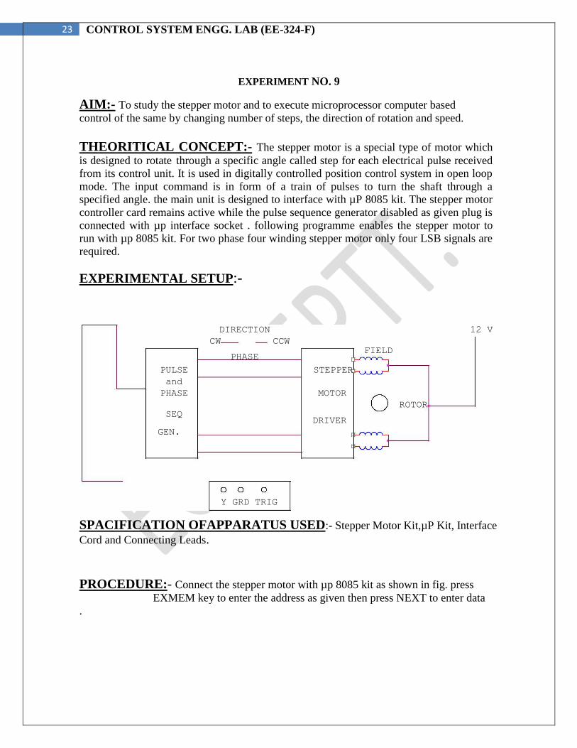
AIM:- To study the stepper motor and to execute microprocessor computer based control of the same by changing number of steps, the direction of rotation and speed.

THEORITICAL CONCEPT:- The stepper motor is a special type of motor which

is designed to rotate through a specific angle called step for each electrical pulse received

from its control unit. It is used in digitally controlled position control system in open loop

mode. The input command is in form of a train of pulses to turn the shaft through a

specified angle. the main unit is designed to interface with µP 8085 kit. The stepper motor

controller card remains active while the pulse sequence generator disabled as given plug is

connected with µp interface socket . following programme enables the stepper motor to

run with µp 8085 kit. For two phase four winding stepper motor only four LSB signals are

required.


DIRECTION

CCW 12 V

CW FIELD

PHASE

PULSE STEPPER

and

MOTOR

PHASE

SEQ ROTOR

DRIVER

GEN.

Y GRD TRIG

SPACIFICATION OFAPPARATUS USED:- Stepper Motor Kit,µP Kit, Interface

Cord and Connecting Leads.

PROCEDURE:- Connect the stepper motor with µp 8085 kit as shown in fig. press EXMEM key to enter the address as given then press NEXT to enter data

.


ADDRESS DATA

2000 3E 80 MVI A,80 Initialize port A as output port.

2002 D3 03 OUT 03 OB

2004 3E F9 Start MVI AFA

2006 D3 00 OUT 00 Output code for step o.

2008 CD 3020 call delay delay between two steps.

200B 3E F5 MVI A, F6 Location reserve for current

Delay.

200d D3 OO OUT OO Output code for step 1.

200F CD 3020 Call delay delay between two steps.

2012 3E F6 MVI A, F5

2014 D3 OO OUT OO Output code for step 2.

2016 CD 3020 calls delay between two steps.

2019 3E FA MVI A, F9.

201B D3 OO OUT OO Output code for step 3.

201D CD 3020 call delay delay between two steps.

2020 C3 04 20 JMP START Start. Press FILL key to store data in memory area. This will complete the pulse sequence

generation. To delay programme route, first press EXMEM to start, a dot sign will appear in

address field then enter the start address. Press NEXT to enter data.

ADDRESS DATA 2030 11 00 00 LXI D 00 00 Generates a delay.

2033 CD BC 03 CALL DELAY

2036 11 00 00 LXI D 00 00 Generates a delay.

2039 CD BC 03 CALL DELAY

203C C9 RET Press FILL to save data.to execute the programme press the key GO .The above programme

is to rotate the motor at a particular as defined by the given address. Changing the following

contents will change the motor speed.

ADDRESS DATA

2030 11 00 20 AND 2036 TO SIMILAR 11 00 20 CHANGE 11 00 10 TO 11 00 10

CHANGE 11 00 05 TO 11 00 05

CHANGE 11 00 03 TO 11 00 03. The motor direction depends upon codes FA, F6 ,F5 AND F9.Change in following codes

will change the motor direction. ADDRESS DATA

2005 3E F9 TO 3E FA

200C 3E F5 TO 3E F6

2012 3E F6 TO 3E F5

2019 3E FA TO 3E F9.


PRECAUTION:- 1. Make the connection of motor with µp kit properly.

2. Feed the programme carefully and correctly.

Do not change the motor direction at high speed.

OBSERVATION DATA:-

Sr No. of Pulses Displacement Step Angle

No.

RESULT AND COMMENTS:- The stepper motor runs as per fed programme.


EXPERIMENT NO. 10 AIM: to study LAG compensator and draw eats magnitude and phase plot.

THEORITICAL CONCEPT: compensation network are often used to make

improvement in transient response and small change in steady state accuracy. The set up

is divided in to three parts. Signal source: It has sine wave of 10-1200 Hz. Of 0-8 Vpp,

Square wave of 20, 40 and 80 Hz of 0-2 Vpp. Trigger is available for trigger of CRO in

external trigger mode. The amplitude is 1.2 Vpp. There are three compensation circuits as

lag, Lead and Lag-Lead with transfer function. The set up has two DC regulated power

supply for signal source and systems. EXPERIMENTAL SETUP

Error Detector

Sine

wave

SQ.

wave

Trig

wave

GAIN 1

GAIN 2

Process

Lag Compensator C R O


SPACIFICATION OF APPARTUS USED: lead lag compensator kit, CRO, and

connecting leads.

PROCEDURE:

The experiment is divided in two parts. 1. Open Loop Response: Connect square wave to gain and CRO across input and

output. Select frequency to 80 Hz at 0.2 Vpp. Measure input amplitude Vpp as A

and output as amplitude as B. Calculate gain factor=B/A. Connect sine wave

with process input, CRO across input and output. Set input voltage =8Vpp. From

low frequency end 10Hz note output voltage Vpp as B. Note the phase difference

for each test frequency. Connect the sine wave with lag input .connect CRO

across input and output. Note the output voltage, phase difference for each test

frequency. Prepare a table between input/output voltage, gain magnitude in db

and phase angle in degrees. Plot a graph accordingly.

2. Close loop response: connect the square wave signal of 20Hz, 1Vpp at input of

error detector. Adjust gain to the value found from plot for required shape of

response and sketch it 0 the paper. From the transient response measure

maximum over shoot Mp, steady state error Ess and peak time Tp. Select wave

frequency to 40Hz, 1Vpp and adjust gain control to 60%. Not gain control setting.

Trace wave form on paper with record of Ess, Mp, and Tp. Select frequency to

80Hz and adjust gain control for minimum Ess 0. Trace wave form with Mp and

Tp. connect process with lag compensator and gain 2. Set square wave frequency

to

20Hz, 1Vpp at error detector input . Adjunct gain control to for similar Ess. Note

gain to from dial setting. Trace the wave form on paper with record of Mp,

Tp and Ess. OBSERVATION DATA :

S.NO. A Vpp B Vpp GAIN dB PHASE ANGLE


GRAPH:

RAO PAHALD SINGH GROUP OF INSTITUTIONS BALANA(MOHINDER ... SYSTEMS lab1_1.pdf · 1 control system...

Documents

Transcript of RAO PAHALD SINGH GROUP OF INSTITUTIONS BALANA(MOHINDER ... SYSTEMS lab1_1.pdf · 1 control system...