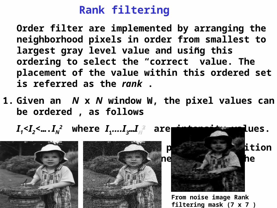
Rank filtering Order filter are implemented by arranging the neighborhood pixels in order from smallest to largest gray level value and using this ordering to select the “correct” value. The placement of the value within this ordered set is referred as the rank .

1. Given an N x N window W, the pixel values can be ordered , as follows

I1<I2<….IN2 where I1….I3…INN22 are intensity values.

2. Select a value from a particular position in the list to use as the new value for the pixel.

From noise image Rank filtering mask (7 x 7 ) rank 4

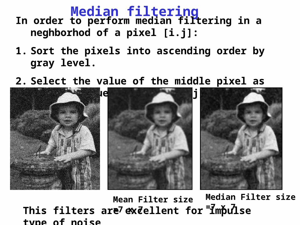
Median filtering In order to perform median filtering in a neghborhod of a

pixel [i.j]:

1. Sort the pixels into ascending order by gray level.

2. Select the value of the middle pixel as the new value for pixel [i.j]

Mean Filter size =7 x 7 Median Filter size =7 x 7

This filters are excellent for impulse type of noise

Median filtering

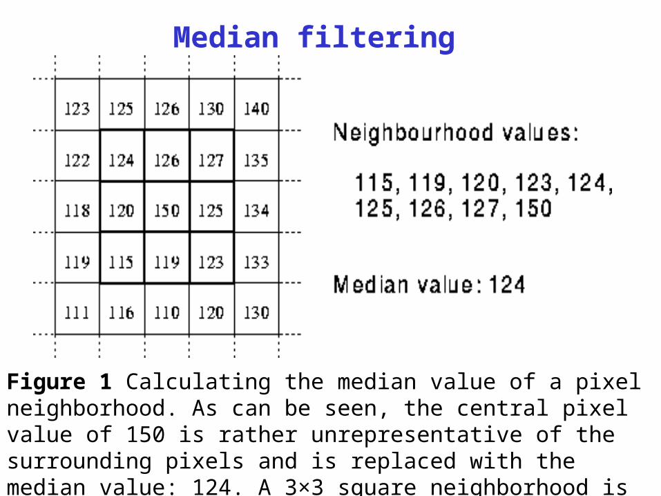
Figure 1 Calculating the median value of a pixel neighborhood. As can be seen, the central pixel value of 150 is rather unrepresentative of the surrounding pixels and is replaced with the median value: 124. A 3×3 square neighborhood is used here --- larger neighborhoods will produce more severe smoothing.

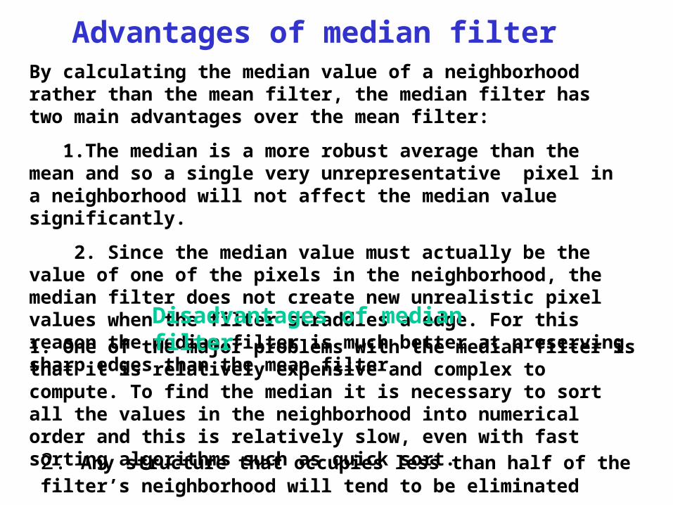
Advantages of median filterBy calculating the median value of a neighborhood rather than the mean filter, the median filter has two main advantages over the mean filter:

1.The median is a more robust average than the mean and so a single very unrepresentative pixel in a neighborhood will not affect the median value significantly.

2. Since the median value must actually be the value of one of the pixels in the neighborhood, the median filter does not create new unrealistic pixel values when the filter straddles a edge. For this reason the median filter is much better at preserving sharp edges than the mean filter.

1. One of the major problems with the median filter is that it is relatively expensive and complex to compute. To find the median it is necessary to sort all the values in the neighborhood into numerical order and this is relatively slow, even with fast sorting algorithms such as quick sort.

Disadvantages of median filter

2. Any structure that occupies less than half of the filter’s neighborhood will tend to be eliminated

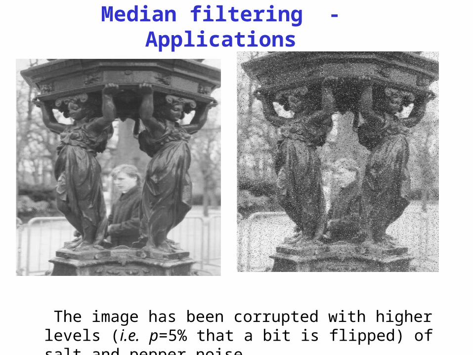
Median filtering - Applications

The image has been corrupted with higher levels (i.e. p=5% that a bit is flipped) of salt and pepper noise

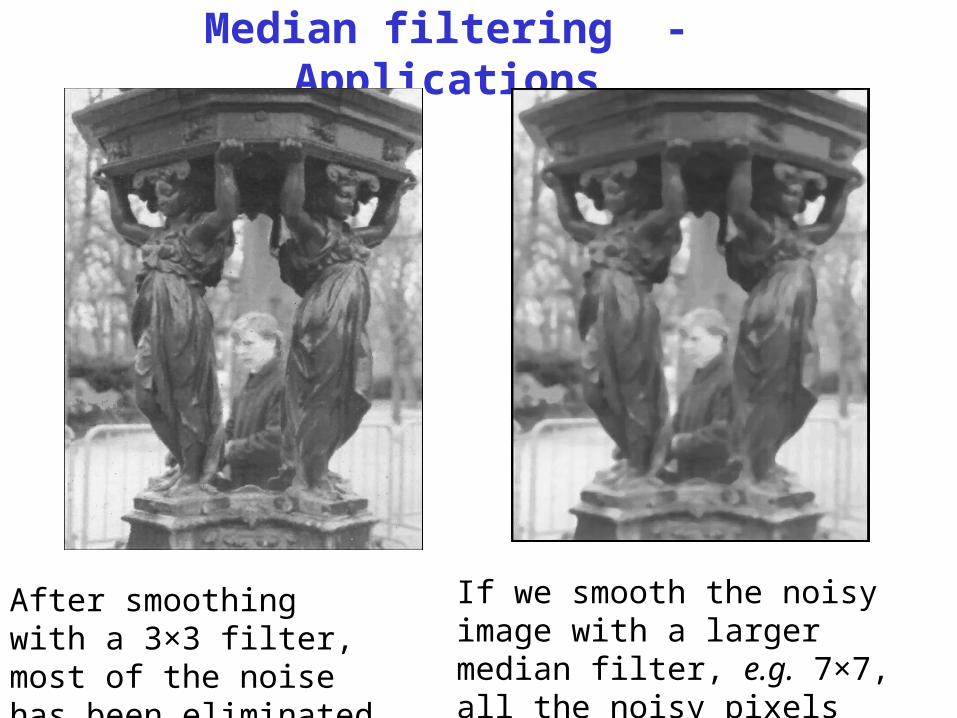
Median filtering - Applications

After smoothing with a 3×3 filter, most of the noise has been eliminated

If we smooth the noisy image with a larger median filter, e.g. 7×7, all the noisy pixels disappear, as shown in this image

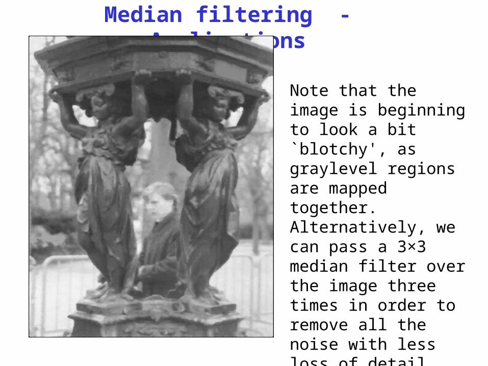
Median filtering - Applications

Note that the image is beginning to look a bit `blotchy', as graylevel regions are mapped together. Alternatively, we can pass a 3×3 median filter over the image three times in order to remove all the noise with less loss of detail

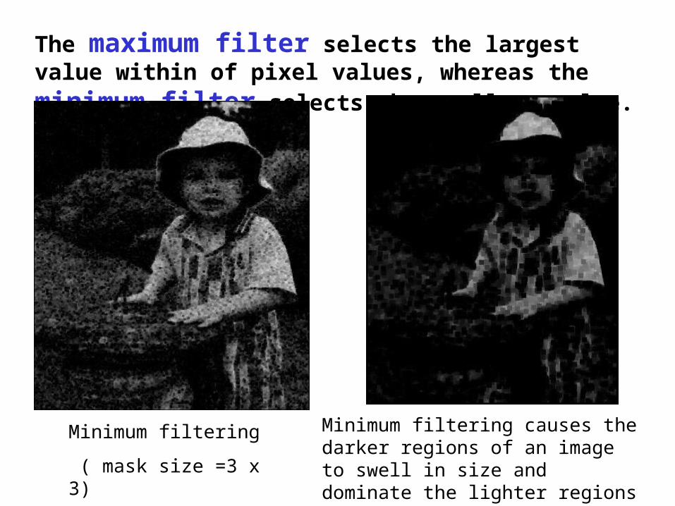
The maximum filter selects the largest value within of pixel

values, whereas the minimum filter selects the smallest value.

Minimum filtering

( mask size =3 x 3)

Minimum filtering causes the darker regions of an image to swell in size and dominate the lighter regions ( mask size =7 x 7)

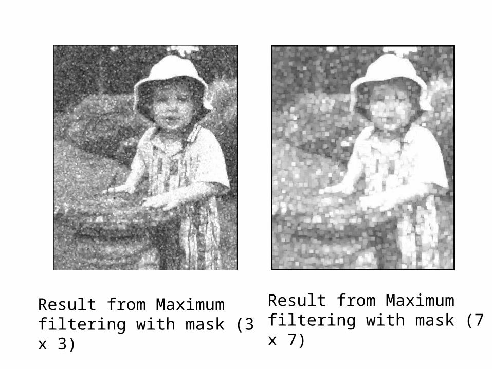
Result from Maximum filtering with mask (3 x 3)

Result from Maximum filtering with mask (7 x 7)

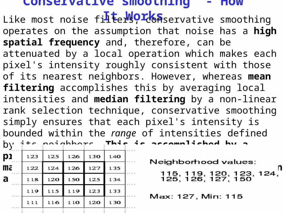
Conservative smoothing - How It WorksLike most noise filters, conservative smoothing operates on the assumption that noise has a high spatial frequency and, therefore, can be attenuated by a local operation which makes each pixel's intensity roughly consistent with those of its nearest neighbors. However, whereas mean filtering accomplishes this by averaging local intensities and median filtering by a non-linear rank selection technique, conservative smoothing simply ensures that each pixel's intensity is bounded within the range of intensities defined by its neighbors. This is accomplished by a procedure which first finds the minimum and maximum intensity values of all the pixels within a windowed region around the pixel in question.

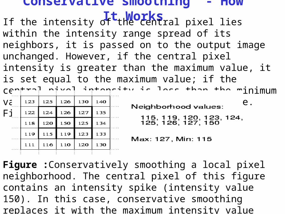
Conservative smoothing - How It WorksIf the intensity of the central pixel lies within the intensity range spread of its neighbors, it is passed on to the output image unchanged. However, if the central pixel intensity is greater than the maximum value, it is set equal to the maximum value; if the central pixel intensity is less than the minimum value, it is set equal to the minimum value. Figure illustrates this idea.

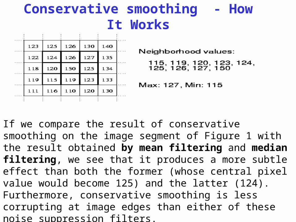
Figure :Conservatively smoothing a local pixel neighborhood. The central pixel of this figure contains an intensity spike (intensity value 150). In this case, conservative smoothing replaces it with the maximum intensity value (127) selected amongst those of its 8 nearest neighbors.

Conservative smoothing - How It Works

If we compare the result of conservative smoothing on the image segment of Figure 1 with the result obtained by mean filtering and median filtering, we see that it produces a more subtle effect than both the former (whose central pixel value would become 125) and the latter (124). Furthermore, conservative smoothing is less corrupting at image edges than either of these noise suppression filters.

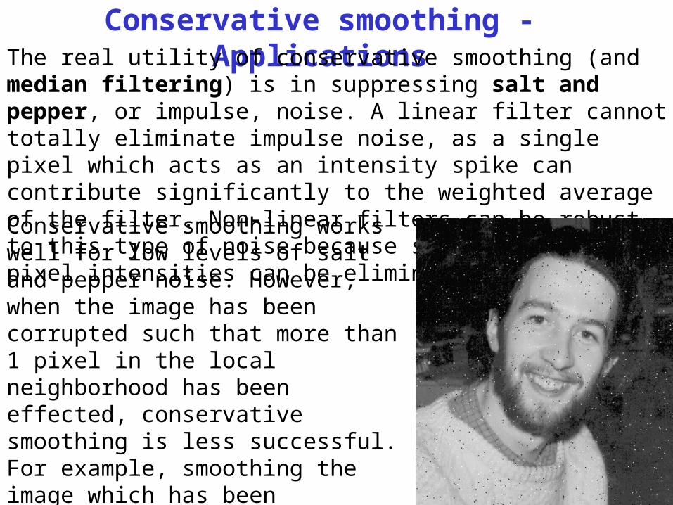
Conservative smoothing - ApplicationsThe real utility of conservative smoothing (and median filtering) is in suppressing salt and pepper, or impulse, noise. A linear filter cannot totally eliminate impulse noise, as a single pixel which acts as an intensity spike can contribute significantly to the weighted average of the filter. Non-linear filters can be robust to this type of noise because single outlier pixel intensities can be eliminated entirely.

Conservative smoothing works well for low levels of salt and pepper noise. However, when the image has been corrupted such that more than 1 pixel in the local neighborhood has been effected, conservative smoothing is less successful. For example, smoothing the image which has been corrupted by 1% salt and pepper noise (i.e. bits have been flipped with probability 1%).

Conservative smoothing - Applications

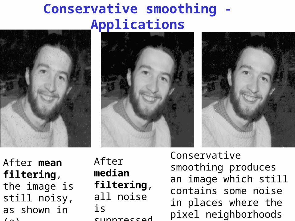
After mean filtering, the image is still noisy, as shown in (a)

After median filtering, all noise is suppressed, as shown in (b)

Conservative smoothing produces an image which still contains some noise in places where the pixel neighborhoods were contaminated by more than one intensity spike.

Conservative smoothing - Applications

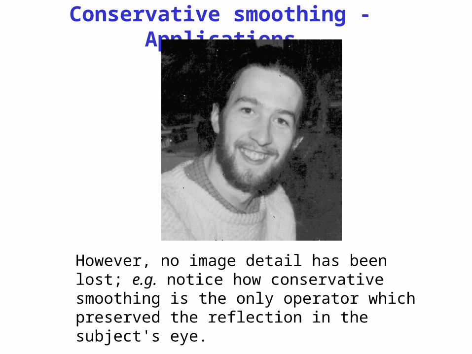
However, no image detail has been lost; e.g. notice how conservative smoothing is the only operator which preserved the reflection in the subject's eye.

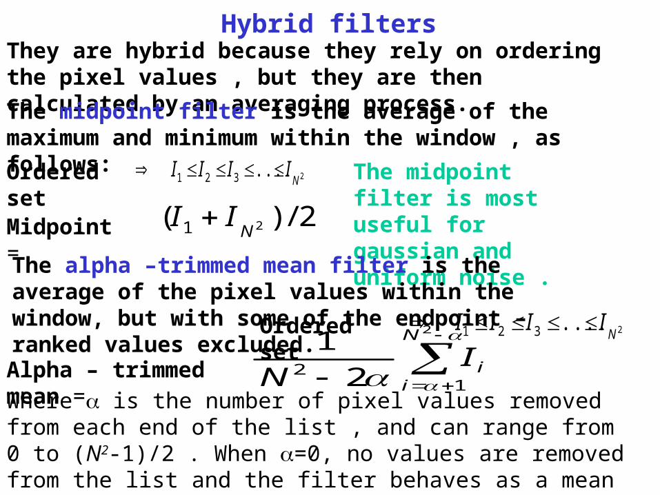
They are hybrid because they rely on ordering the pixel values , but they are then calculated by an averaging process.

The midpoint filter is the average of the maximum and minimum within the window , as follows:

Hybrid filters

Ordered set 2....321 NIIII

Midpoint = 2/)( 21 NII

The midpoint filter is most useful for gaussian and uniform noise .

The alpha –trimmed mean filter is the average of the pixel values within the window, but with some of the endpoint –ranked values excluded. Ordered set 2....321 N

IIII

Alpha – trimmed mean =

2

12 2

1 N

iiI

NWhere is the number of pixel values removed from each end of the list , and can range from 0 to (N2-1)/2 . When =0, no values are removed from the list and the filter behaves as a mean filter. If =(N2-1)/2 , the equation becomes a median filter.

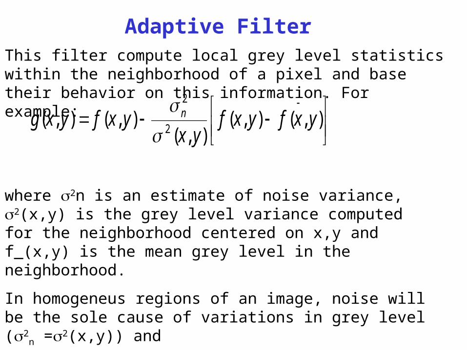
Adaptive Filter

where 2n is an estimate of noise variance, 2(x,y) is the grey level variance computed for the neighborhood centered on x,y and f_(x,y) is the mean grey level in the neighborhood.

In homogeneus regions of an image, noise will be the sole cause of variations in grey level (2

n =2(x,y)) and

g(x,y) = f_(x,y)

This filter compute local grey level statistics within the neighborhood of a pixel and base their behavior on this information. For example:

),(),(),(

),(),(2

2

yxfyxfyx

yxfyxg n

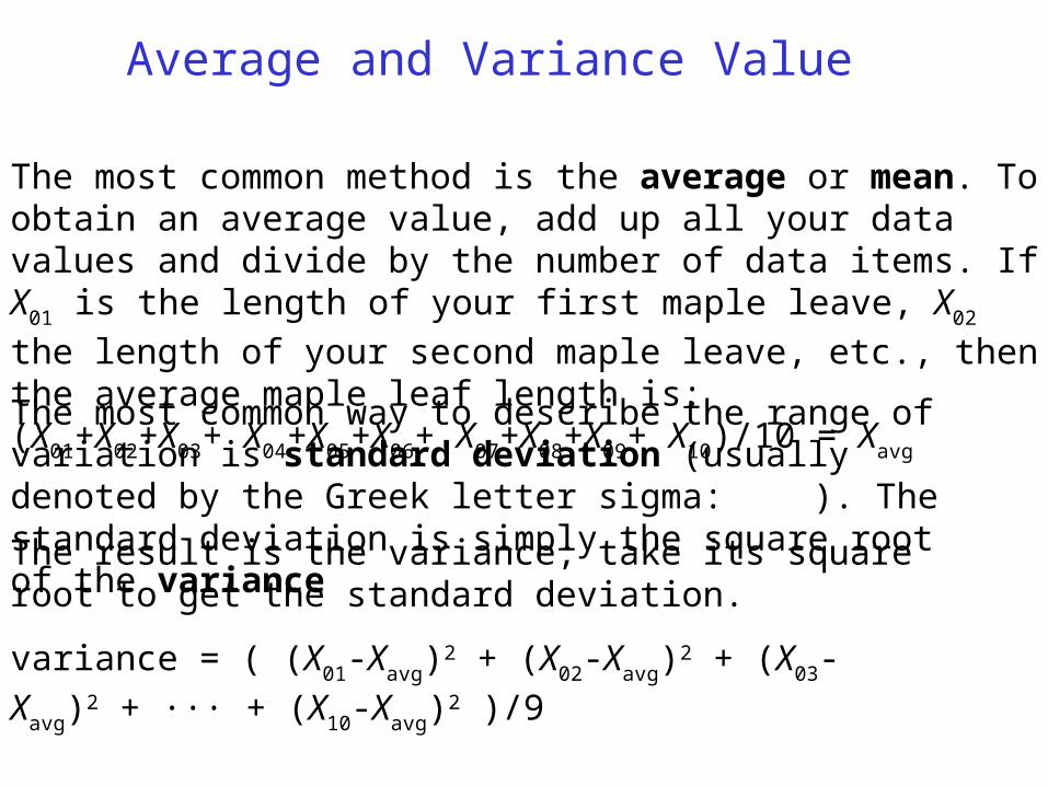
Average and Variance Value

The most common method is the average or mean. To obtain an average value, add up all your data values and divide by the number of data items. If X01 is the length of your first maple leave, X02 the length of your

second maple leave, etc., then the average maple leaf length is: (X01+X02+X03+ X04+X05+X06+ X07+X08+X09+ X10)/10 = Xavg

The most common way to describe the range of variation is standard deviation (usually denoted by the Greek letter sigma:   ). The standard deviation is simply the square root of the variance

The result is the variance; take its square root to get the standard deviation.

variance = ( (X01-Xavg)2 + (X02-Xavg)

2 + (X03-Xavg)2 + ··· + (X10-Xavg)

2

)/9

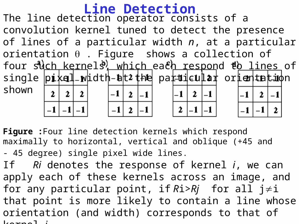
Line DetectionThe line detection operator consists of a convolution kernel tuned to detect the presence of lines of a particular width n, at a particular orientation . Figure shows a collection of four such kernels, which each respond to lines of single pixel width at the particular orientation shown

Figure :Four line detection kernels which respond maximally to horizontal, vertical

and oblique (+45 and - 45 degree) single pixel wide lines.

If Ri denotes the response of kernel i, we can apply each of these kernels across an image, and for any particular point, if Ri>Rj for all ji that point is more likely to contain a line whose orientation (and width) corresponds to that of kernel i.

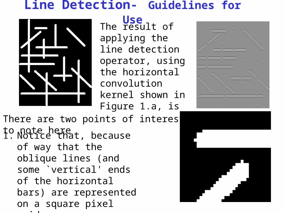
Line Detection- Guidelines for UseThe result of applying the line detection operator, using the horizontal convolution kernel shown in Figure 1.a, is

There are two points of interest to note here

1. Notice that, because of way that the oblique lines (and some `vertical' ends of the horizontal bars) are represented on a square pixel grid, e.g.

Line Detection- Guidelines for Use

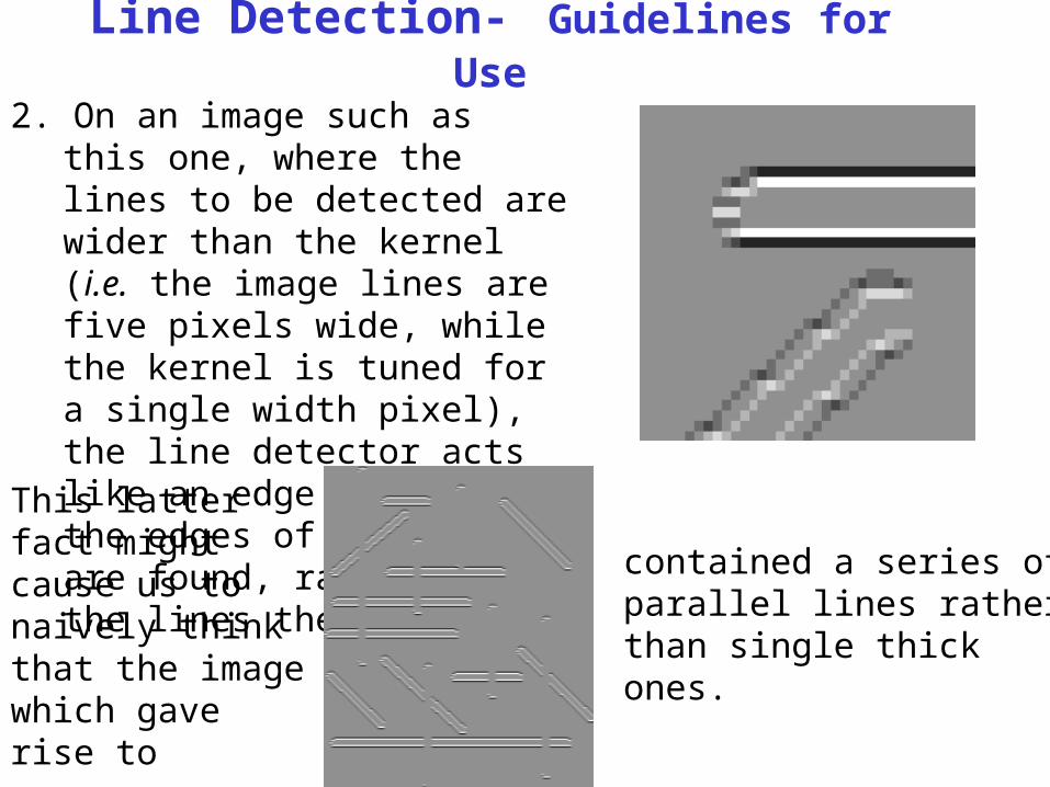
2. On an image such as this one, where the lines to be detected are wider than the kernel (i.e. the image lines are five pixels wide, while the kernel is tuned for a single width pixel), the line detector acts like an edge detector: the edges of the lines are found, rather than the lines themselves.

This latter fact might cause us to naively think that the image which gave rise to

contained a series of parallel lines rather than single thick ones.

Line Detection- Guidelines for Use

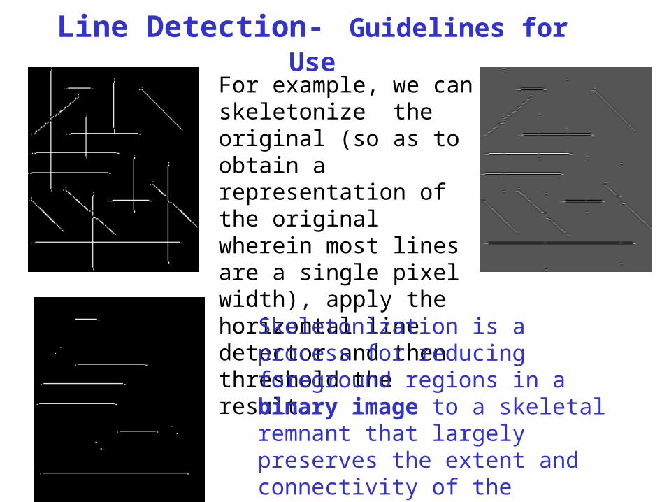
For example, we can skeletonize the original (so as to obtain a representation of the original wherein most lines are a single pixel width), apply the horizontal line detector and then threshold the result.

Skeletonization is a process for reducing foreground regions in a binary image to a skeletal remnant that largely preserves the extent and connectivity of the original region while throwing away most of the original foreground pixels.

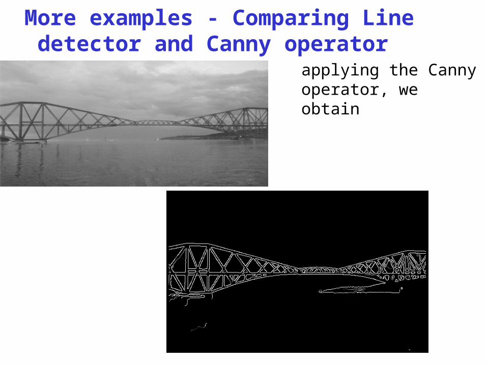
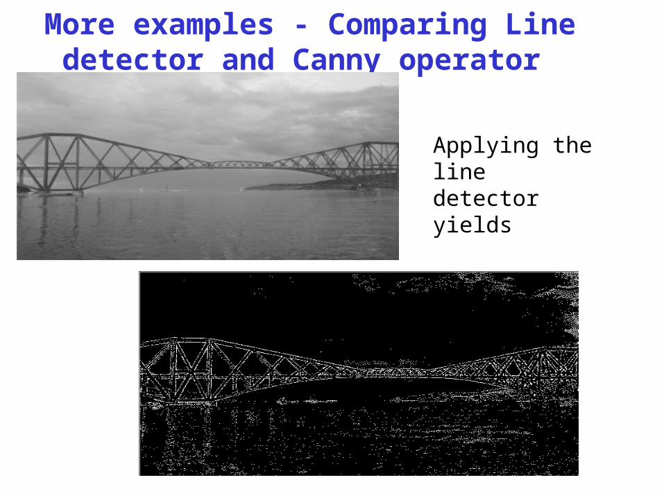
More examples - Comparing Line detector and Canny operator

applying the Canny operator, we obtain

More examples - Comparing Line detector and Canny operator

Applying the line detector yields

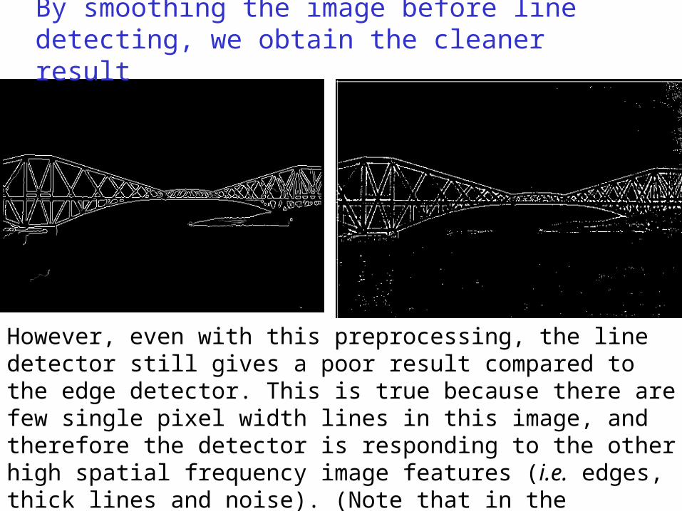
By smoothing the image before line detecting, we obtain the cleaner result

However, even with this preprocessing, the line detector still gives a poor result compared to the edge detector. This is true because there are few single pixel width lines in this image, and therefore the detector is responding to the other high spatial frequency image features (i.e. edges, thick lines and noise). (Note that in the previous example, the image contained the feature that the kernel was tuned for and therefore we were able to threshold away the weaker kernel response to edges.)

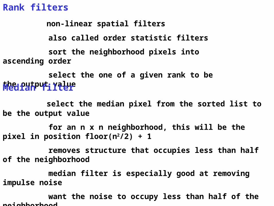
Rank filters

non-linear spatial filters

also called order statistic filters

sort the neighborhood pixels into ascending order

select the one of a given rank to be the output value

Median filter

select the median pixel from the sorted list to be the output value

for an n x n neighborhood, this will be the pixel in position floor(n2/2) + 1

removes structure that occupies less than half of the neighborhood

median filter is especially good at removing impulse noise

want the noise to occupy less than half of the neighborhood

can increase the neighborhood size for noisier images

the shape of the neighborhood can affect amount of damage to object edges

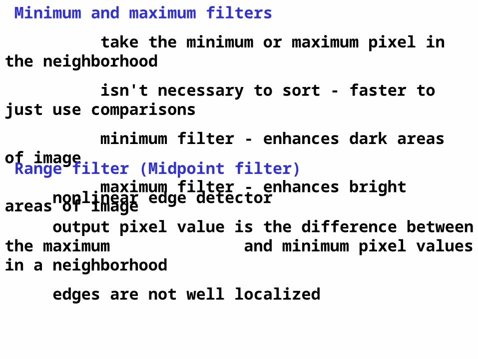
Minimum and maximum filters

take the minimum or maximum pixel in the neighborhood

isn't necessary to sort - faster to just use comparisons

minimum filter - enhances dark areas of image

maximum filter - enhances bright areas of image

Range filter (Midpoint filter)

nonlinear edge detector

output pixel value is the difference between the maximum and minimum pixel values in a neighborhood

edges are not well localized

Alpha-trimmed mean filter

a hybrid of linear and nonlinear approaches

sort the neighborhood pixels into ascending order

discard a given number (alpha) from each end of the list

output pixel is the mean of the remaining pixel values

alpha = 0 gives a mean filter

alpha = (n2 - 1)/2 gives a median filter

Minimal mean square error filter

adaptive filter - behavior depends on local image properties

must supply an estimate of noise variance

at each pixel, compute the mean gray-level and gray-level variance of neighborhood

ratio of noise variance estimate to gray-level variance in neighborhood affects

computation of output pixel

where neighborhood variance equals noise variance, output is the mean gray-level

where neighborhood variance is large compared to noise variance (near edges),

output is close to input pixel value