Range Reporting of Planar Convex Hull and Skyline Points

Thesis submitted in partial fulfillmentof the requirements for the degree of

MS by Researchin

Computer Science Engineering

by

NADEEM MOIDU200802025

nadeem.moiduug08@students.iiit.ac.in

International Institute of Information TechnologyHyderabad - 500 032, INDIA

July 2015

Copyright c© Nadeem Moidu, 2015

All Rights Reserved

International Institute of Information TechnologyHyderabad, India

CERTIFICATE

It is certified that the work contained in this thesis, titled ’Range Reporting of Planar Convex Hull andMaxima Points’ by Nadeem Moidu, has been carried out under my supervision and is not submittedelsewhere for a degree.

Date Adviser: Dr. Kishore Kothapalli

Acknowledgments

First and foremost, I would like to express my sincere gratitude to my advisor, Dr. Kishore Kotha-palli, without whose guidance and motivation, I would not have been able to do this thesis in my favoritefield of algorithms and data structures. I would like to thank my committee members, Dr. ProsenjitGupta and Dr. Indranil Chakrabarty for their support and suggestions.

I would like to thank my algorithms professor, Dr. Kannan Srinathan with whom I discussed variousideas, both technical and others, over several years. My friends, Jatin Agarwal, Sankalp Khare andAnish Shankar who helped shape my ideas into proper algorithms and proof reading most of my papers.A lot of other friends have also been part my journey: Shashank, Tushar, Aman, Vyas, Basil, Aseem,Mihir, Sanidhya, Jaspal, Apoorv, Ashok, Sai Ganesh, Anirban, Jay, Neeraj, Mohit, Kunal, Yash and somany others.

I have received inspiration and motivation in various forms throughout my life from my parents,Moidu and Safiya, as well as my brother, Nabeel, and my sister, Nawal.

I thank God, for always being there for me.

iv

Abstract

Computational geometry is the branch of computer science which deals with computation of geo-metric functions. It has applications to various fields of computer science such as computer graphics,robotics, VLSI, etc. Range query problems are a set of problems where data structure has to be designedto preprocess the input such that given a query range, an operation has to be supported on that particularrange of inputs. These problems are significant today because the huge amount of data makes it relevantto have small subsets of it ready to be queried.

We consider the planar convex hull range query problem. Convex hull is an important geometricconstruct because it is performed as a preprocessing step for a large class of problems. Let P be a setof points in the plane. We preprocess these points into a data structure such that given an orthogonalrange query, we can report the convex hull of the points in the range in O(log2 n + h) time, where h isthe size of the output. The data structure uses O(n log n) space. This improves the previous bound ofO(log5 n + h) time and O(n log2 n) space. Given a range query, it also supports extreme points in agiven direction, tangent queries through a given point, and line-hull intersection queries on the points inthe range in time O(log2 n) for each orthogonal query and O(log n) time for each additional query onthat range. These bounds are independent of h, the number of points on the hull. These problems havenot been studied before.

We also consider the generalized reporting versions of the planar range maxima problem. We solvethe planar range maxima problem for two-sided, three-sided and four-sided queries. We achieve a querytime of O(log n + c) using O(n) space for the two-sided case, where n denotes the number of storedpoints and c the number of colors reported. For the three-sided case, we achieve query time O(log2 n+

c log n) using O(n) space while for four-sided queries we answer queries in O(log3 n+ c log2 n) usingO(n log n) space.

v

Publications

List of Publications

1. Nadeem Moidu, Jatin Agarwal and Kishore Kothapalli. Planar Convex Hull Range Query andRelated Problems. Appeared, 25th Canadian Conference on Computational Geometry, CCCG2013.

2. Nadeem Moidu, Jatin Agarwal and Kannan Srinathan. On Generalized Planar Skyline and ConvexHull Range Queries. 7th International Workshop on Algorithms and Computation, WALCOM2014

3. Sankalp Khare, Jatin Agarwal, Nadeem Moidu and Kannan Srinathan. Improved bounds forSmallest Enclosing Disk Range Queries. 26th Canadian Conference on Computational Geometry2014.

vi

Contents

Chapter Page

1 Introduction . . . . . . . . . . . . . . . . . . . . . . . . . . . . . . . . . . . . . . . . . . 11.1 Computational Geometry . . . . . . . . . . . . . . . . . . . . . . . . . . . . . . . . . 11.2 Range Queries . . . . . . . . . . . . . . . . . . . . . . . . . . . . . . . . . . . . . . . 11.3 Online and Offline Algorithms . . . . . . . . . . . . . . . . . . . . . . . . . . . . . . 31.4 Output Sensitivity . . . . . . . . . . . . . . . . . . . . . . . . . . . . . . . . . . . . . 31.5 Preprocessing for Geometric Problems . . . . . . . . . . . . . . . . . . . . . . . . . . 41.6 Convex Hull . . . . . . . . . . . . . . . . . . . . . . . . . . . . . . . . . . . . . . . . 41.7 Skyline Points . . . . . . . . . . . . . . . . . . . . . . . . . . . . . . . . . . . . . . . 61.8 Generalized Range Query . . . . . . . . . . . . . . . . . . . . . . . . . . . . . . . . . 71.9 Structure of the Thesis . . . . . . . . . . . . . . . . . . . . . . . . . . . . . . . . . . 7

2 Fundamentals . . . . . . . . . . . . . . . . . . . . . . . . . . . . . . . . . . . . . . . . . 82.1 Model of Computation . . . . . . . . . . . . . . . . . . . . . . . . . . . . . . . . . . 82.2 Range Trees . . . . . . . . . . . . . . . . . . . . . . . . . . . . . . . . . . . . . . . . 92.3 Heavy-Light Decomposition . . . . . . . . . . . . . . . . . . . . . . . . . . . . . . . 92.4 Binary Search on Functions . . . . . . . . . . . . . . . . . . . . . . . . . . . . . . . . 10

3 Planar Convex Hull Range Queries . . . . . . . . . . . . . . . . . . . . . . . . . . . . . . . 113.1 Introduction . . . . . . . . . . . . . . . . . . . . . . . . . . . . . . . . . . . . . . . . 113.2 Basic Solution . . . . . . . . . . . . . . . . . . . . . . . . . . . . . . . . . . . . . . . 123.3 Motivation . . . . . . . . . . . . . . . . . . . . . . . . . . . . . . . . . . . . . . . . . 143.4 Data Structure . . . . . . . . . . . . . . . . . . . . . . . . . . . . . . . . . . . . . . . 163.5 Preprocessing . . . . . . . . . . . . . . . . . . . . . . . . . . . . . . . . . . . . . . . 173.6 Query Algorithm . . . . . . . . . . . . . . . . . . . . . . . . . . . . . . . . . . . . . 19

3.6.1 Other Problems . . . . . . . . . . . . . . . . . . . . . . . . . . . . . . . . . . 203.7 Summary . . . . . . . . . . . . . . . . . . . . . . . . . . . . . . . . . . . . . . . . . 21

4 Generalized Maxima Range Queries . . . . . . . . . . . . . . . . . . . . . . . . . . . . . . 224.1 Introduction . . . . . . . . . . . . . . . . . . . . . . . . . . . . . . . . . . . . . . . . 224.2 Applications . . . . . . . . . . . . . . . . . . . . . . . . . . . . . . . . . . . . . . . . 224.3 Previous Work . . . . . . . . . . . . . . . . . . . . . . . . . . . . . . . . . . . . . . . 234.4 Preliminaries . . . . . . . . . . . . . . . . . . . . . . . . . . . . . . . . . . . . . . . 23

4.4.1 Generalized Reporting . . . . . . . . . . . . . . . . . . . . . . . . . . . . . . 234.4.2 Heavy Light Decomposition . . . . . . . . . . . . . . . . . . . . . . . . . . . 24

4.4.2.1 Preprocessing . . . . . . . . . . . . . . . . . . . . . . . . . . . . . 24

vii

viii CONTENTS

4.4.2.2 Query . . . . . . . . . . . . . . . . . . . . . . . . . . . . . . . . . 254.5 Generalized Maxima Queries . . . . . . . . . . . . . . . . . . . . . . . . . . . . . . . 25

4.5.1 Two Sided Queries . . . . . . . . . . . . . . . . . . . . . . . . . . . . . . . . 254.5.2 Three Sided Queries . . . . . . . . . . . . . . . . . . . . . . . . . . . . . . . 254.5.3 Four Sided Query . . . . . . . . . . . . . . . . . . . . . . . . . . . . . . . . . 27

4.6 Summary . . . . . . . . . . . . . . . . . . . . . . . . . . . . . . . . . . . . . . . . . 28

5 Conclusions . . . . . . . . . . . . . . . . . . . . . . . . . . . . . . . . . . . . . . . . . . 29

Bibliography . . . . . . . . . . . . . . . . . . . . . . . . . . . . . . . . . . . . . . . . . . . . 31

List of Figures

Figure Page

1.1 In range queries, some function has to be computed on the subset of P which is insidethe query region q. . . . . . . . . . . . . . . . . . . . . . . . . . . . . . . . . . . . . 2

1.2 Voronoi diagram for a set of points. The outer lines extend infinitely. . . . . . . . . . . 41.3 Convex hull for a set of points. . . . . . . . . . . . . . . . . . . . . . . . . . . . . . . 51.4 Skyline of a set of points. . . . . . . . . . . . . . . . . . . . . . . . . . . . . . . . . . 6

3.1 The hull can be divided into 4 parts based on the extreme points as shown. . . . . . . . 133.2 When the hulls are stored in a standard 2D range tree, the query divisions are as shown. 133.3 The shaded regions can be discarded before the combination step. . . . . . . . . . . . 143.4 We may not discard any region and end up with O(log2 n) regions still. . . . . . . . . 153.5 Example of how a query is split into canonical node regions for (a) normal 2D range

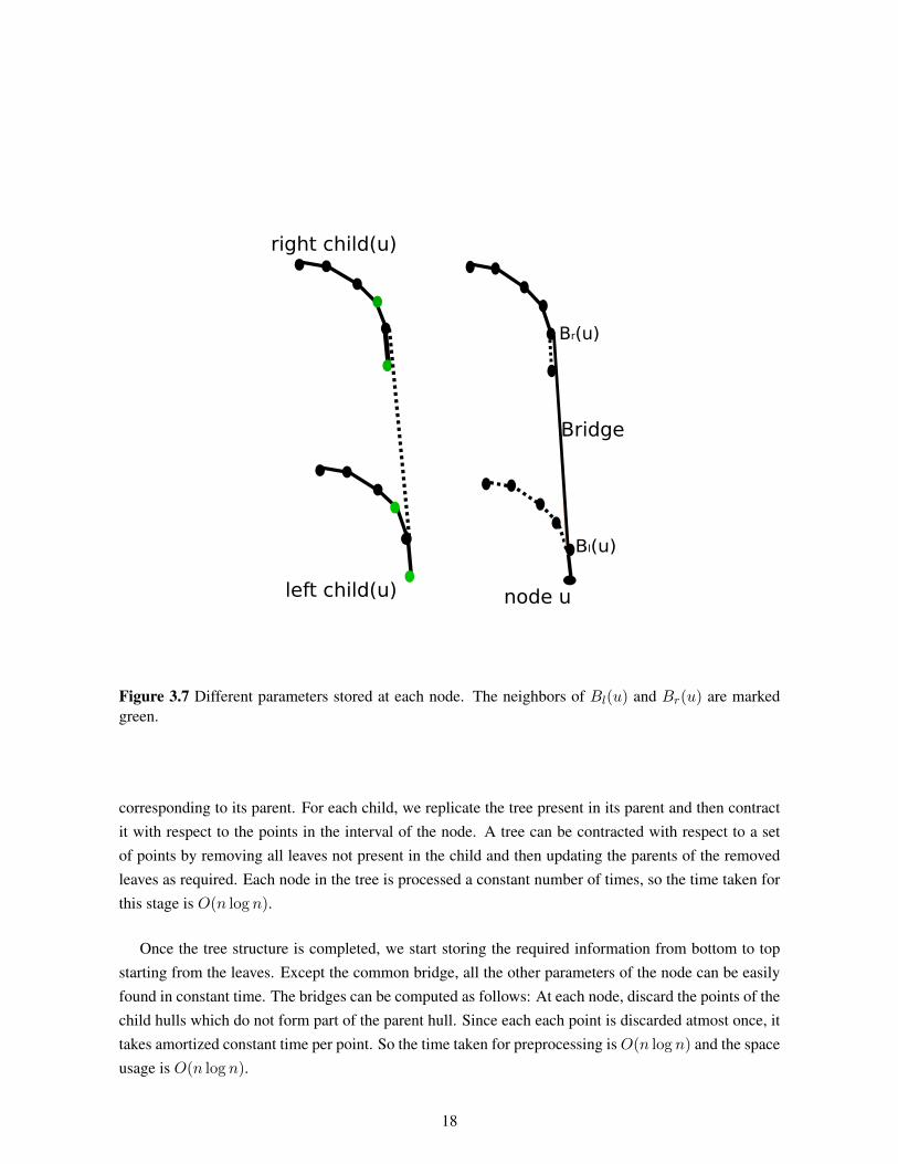
tree and (b) our tree . . . . . . . . . . . . . . . . . . . . . . . . . . . . . . . . . . . . 163.6 Original tree and the contracted tree for the set {a,c,d,f} . . . . . . . . . . . . . . . . . 163.7 Different parameters stored at each node. The neighbors of Bl(u) and Br(u) are marked

green. . . . . . . . . . . . . . . . . . . . . . . . . . . . . . . . . . . . . . . . . . . . 183.8 Example of a query. The candidate blocks have been darkened. . . . . . . . . . . . . . 20

ix

List of Tables

Table Page

5.1 Summary of our results . . . . . . . . . . . . . . . . . . . . . . . . . . . . . . . . . . 29

x

Chapter 1

Introduction

1.1 Computational Geometry

Geometry is the study of shape, size, relative position of figures and the properties of space. Earlystudies of geometry was mainly concerned with lengths, areas and volumes of objects. The field hasnow expanded to topics like differential geometry, topology, algebraic geometry, etc.

Computational geometry is the branch of computer science devoted to the study of algorithms whichinvolves geometry. Various geometric problems arise in different fields of computer science. Com-puter graphics represents images using points and lines and do operations on it like image rendering.Robotics require the best path for the robot to move given the current positions of near by objects. Inte-grated circuit design largely relies on geometric problems to minimize the area required for the design.Geographic Information Systems (GIS) involves a lot of location based searching and route planning.

Apart from the direct application such as the ones mentioned above, we also have problems in otherfields which can be converted to problems in geometry. For example, a database table with two nu-merical parameters can be considered as a set of points. In certain cases, this conversion is not sostraightforward. Consider the following problem: Given a one dimensional array of numbers, prepro-cess it into a data structure which supports queries of the form: ”Given an contiguous subsequenceof the array, report the number of distinct numbers in that subsequence”. This can be converted intoa range reporting problem in two dimensions and solved using geometric methods. This problem hasbeen extensively used in this thesis.

1.2 Range Queries

Range query data structures are those which support operations on a subset of the point set. e.g.,You have a one dimensional array, A, preprocess it such that queries of the following form can bequickly reported, ”Given a query [low, high], report the sum of all values, Ai, where low ≤ i ≤ high”.Range queries often come up in the various geometry related fields mentioned earlier, such as databases,

1

robotics, etc. The following database query can be considered a range query and solved efficiently usinggeometric data structures.

SELECT VALUE, PRICE FROM PRODUCTS WHERE VALUE > 100 AND PRICE < 1000;

Here (VALUE, PRICE) can be considered as a point. So this data base query corresponds to the orthog-onal range reporting problem.

P

q

Figure 1.1 In range queries, some function has to be computed on the subset of P which is inside thequery region q.

One of the main range query problems studied is the range minimum query (RMQ) problem. Asthe name states, the problem is to find the position of the minimum number in a range, usually in aone dimensional array. The ”Recursive Star-Tree Parallel Data Structure” [4] by Berkman and Vishkinintroduced a new approach to solve the problem. Note that only the position of the minimum has to bereported, and not the actual value. This enables us to avoid storing the array and only storing enoughinformation to report the position. Fischer and Heun showed that only 2n + o(n) bits are required toanswer this query in constant time [14]. They also proved that at least 2n − o(n) bits are required forthe same.

In a range query, the range may be represented in any form, e.g., polygon, circle, etc. It can also bea rectangle that is not parallel to the axes. However, in this thesis, we will only deal with orthogonalrange queries, i.e., the range will always be defined by axis parallel lines. Orthogonal queries are ofteneasier to process because each dimension can be handled separately.

Some of the other recently studied range query problems include range mode and range median,which were solved by Chan [13] and Brodal [7] respectively.

2

1.3 Online and Offline Algorithms

An online algorithm is one where the input is processed one by one without waiting to receive theentire data set. An offline algorithm is one where the data processing starts only after receiving thecomplete data. In the case of sorting, insertion sort is considered an online algorithm since it maintainsthe available values in sorted order before starting to the process the next value. On the other hand,selection sort is an offline algorithm since it cannot start before receiving all the values. Having thecomplete input beforehand is considered an extra resource, since it can simplify certain problems, e.g.,compressing a video is easier and can be done more efficiently if the complete video is available asopposed to compressing a video stream on the fly.

In range query problems, an algorithm is usually called offline if it takes all the queries before givingthe output even for the first one. This method is not preferred because it does not suit most practicalscenarios. However, it is still used if an online algorithm for the same is found to be difficult. Solvingthe dynamic convex hull problem in O(log n) time was considered an open problem for a long time.The first such algorithm to be proposed was an offline one by Hershberger and Suri [17]. The problemwas later solved by Jacob and Brodal [6] in amortized O(log n) time, but achieving that in the worstcase still remains open.

All the algorithms discussed in this thesis are online algorithms.

1.4 Output Sensitivity

The output of a range query is often a subset of the point set. If k is the size of the output, thenreporting the output alone takes O(k) time. It is possible that k = Θ(n), where n is the size of thecomplete point set. In this case, the reporting takes O(n), which could be the time taken for a trivialalgorithm. However, if k = o(n), then we could have some algorithm which takes only time whichis polynomial in k and log n. It is still relevant to study such algorithms. So it is important to have aparameter in the time complexity which is the size of the output. This concept of having the algorithmdepend on the output size is called output sensitivity. Range query algorithms usually have complexityof the form O(f(n) + kg(n)), where f(n) and g(n) are normally o(n), typically O(polylog(n)).

If the range query is a function of a subset of the point set with only one numerical value as theoutput, then it should not have a dependence on k which is the size of the subset on which the functionis computed. For instance, if the sum of values in a range in an array is to be computed, then anyalgorithm which goes through all those values in that range will not be considered output sensitive. Thesize of the output in this case is O(1), so the time complexity of the algorithm should only depend on n.

3

1.5 Preprocessing for Geometric Problems

Any query based problem requires some preprocessing. However, problems in geometry have anadditional advantage that some common preprocessing structures can solve a very large set of problems.These include Voronoi diagrams, Delaunay triangulation, convex hulls, etc.

The Voronoi diagram [3] of a set of points, P , is the division of the plane into regions such that eachpoint, Pi has a region corresponding to it, which is the set of all points on the plane for which the closestpoint in P is Pi. See 1.2. It has practical applications in robotics, machine learning, computationalchemistry, climatology, etc. The Voronoi diagram of a set of n points can be constructed in O(n log n)

time and stored in O(n) space. In geometry, it is mostly used for the nearest neighbor query, i.e., givena query point, find the point in P closest to it. It can also solve problems such as large empty circle, etc.Delaunay triangulation is the dual of Voronoi diagram.

Figure 1.2 Voronoi diagram for a set of points. The outer lines extend infinitely.

1.6 Convex Hull

The convex hull of a set of points is the convex figure with the minimum area which includes all thepoints in the given set. A simple experiment which conveys this definition is as follows: Fix a few nailson a table. Take an elastic band and spread it outside all the points. The band will converge such that it

4

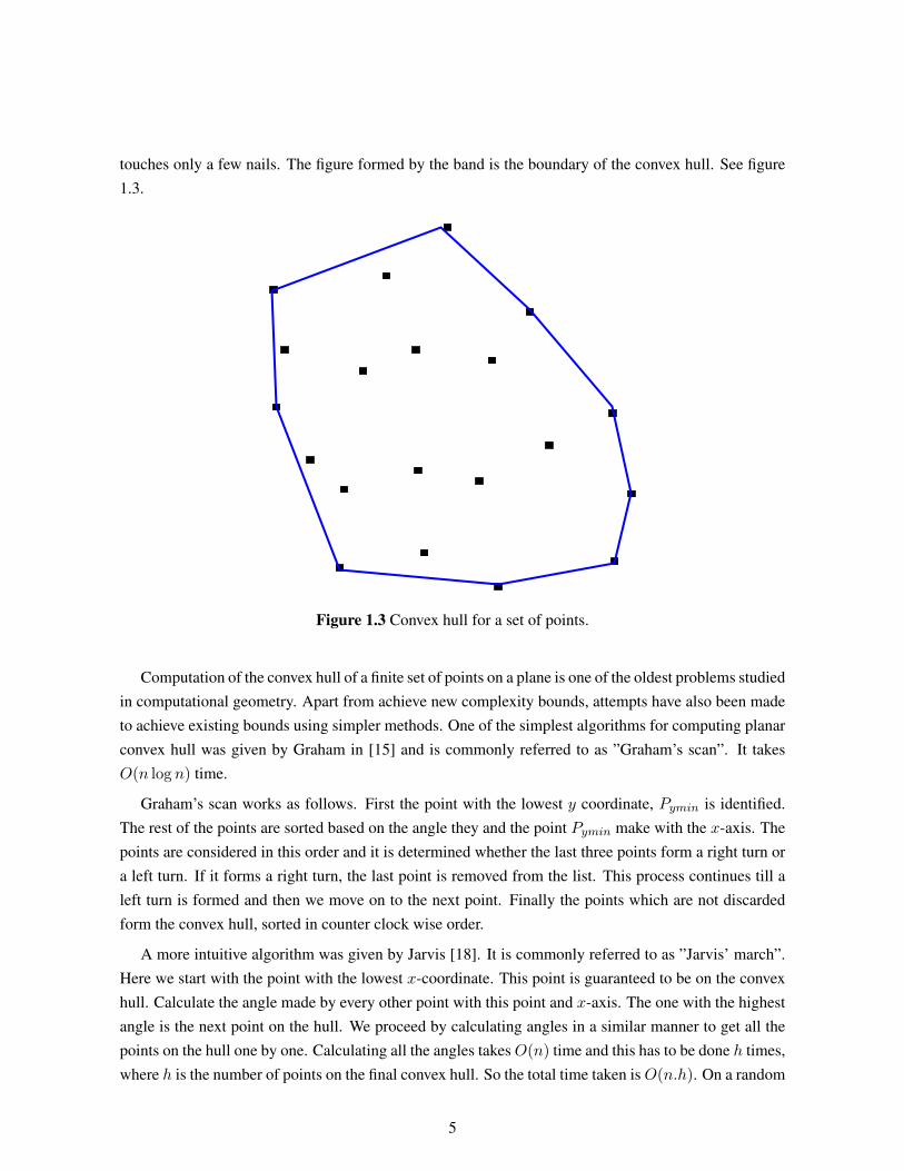
touches only a few nails. The figure formed by the band is the boundary of the convex hull. See figure1.3.

Figure 1.3 Convex hull for a set of points.

Computation of the convex hull of a finite set of points on a plane is one of the oldest problems studiedin computational geometry. Apart from achieve new complexity bounds, attempts have also been madeto achieve existing bounds using simpler methods. One of the simplest algorithms for computing planarconvex hull was given by Graham in [15] and is commonly referred to as ”Graham’s scan”. It takesO(n log n) time.

Graham’s scan works as follows. First the point with the lowest y coordinate, Pymin is identified.The rest of the points are sorted based on the angle they and the point Pymin make with the x-axis. Thepoints are considered in this order and it is determined whether the last three points form a right turn ora left turn. If it forms a right turn, the last point is removed from the list. This process continues till aleft turn is formed and then we move on to the next point. Finally the points which are not discardedform the convex hull, sorted in counter clock wise order.

A more intuitive algorithm was given by Jarvis [18]. It is commonly referred to as ”Jarvis’ march”.Here we start with the point with the lowest x-coordinate. This point is guaranteed to be on the convexhull. Calculate the angle made by every other point with this point and x-axis. The one with the highestangle is the next point on the hull. We proceed by calculating angles in a similar manner to get all thepoints on the hull one by one. Calculating all the angles takes O(n) time and this has to be done h times,where h is the number of points on the final convex hull. So the total time taken is O(n.h). On a random

5

set of points, it can be shown that the number of points on the hull is O(n), so the two algorithms arenot easily comparable.

The most efficient convex hull computation algorithm was provided by Kirkpatrick and Seidel in[20]. It was called the ”ultimate planar convex hull algorithm” since it achieved the lowest boundpossible of O(n log h). However, a simpler algorithm which achieves the same bound was given byChan in [9]. Both algorithms use the divide and conquer strategy. We will not discuss this in moredetail.

The problem of maintaining the convex hull of a dynamic set of points under insertion and/or deletionhas also been studied. The first algorithm was provided by Overmars and van Leeuwen in [21]. Theysupported both addition and deletion in O(log2 n) time. The most efficient data structure for the sametill now was given by Jacob and Brodal in [6] which supports maintaining the hull and addition anddeletion of points in amortized O(log n) time.

1.7 Skyline Points

A point Pi is said to dominate a point Pj if the each coordinate of Pi is greater than the correspondingcoordinate of Pj . For simplicity, we will assume that all coordinates are distinct. Skyline points (alsocalled maximal points) are the subset of points which are not dominated by any other point. They areimportant in many fields for pruning the input, getting samples, etc. See figure 1.4.

Figure 1.4 Skyline of a set of points.

6

Finding the skyline of a static finite set of points on a plane is simple. Sort the points by in non-increasing order of their x coordinate. Keep track of the maximum y coordinate encountered and processthe points as follows: If a new maximum y coordinate is encountered, update the maximum and reportthe point as part of the skyline. Else, ignore the point. The reported points form the skyline in non-increasing order of y-coordinates.

Dynamic skyline computation was first done by Overmars and van Leeuwen in [21]. Most methodsused for convex hull computation can be used to compute skyline also. However, it is an overkill sincesimpler methods are usually available. For example, the methods used in this thesis for computing theconvex hull in a range can be applied for skylines, but more efficient algorithms have been proposed forthe same.

1.8 Generalized Range Query

Here we consider a set of points where each point has a color associated with it. In a generalizedrange query problem we have to report the colorwise information about the problem. For example,the range counting problem counts the number of points in the range. The generalized range countingproblem (also called colored or categorical range reporting) counts the number of distinct colors in therange. The problem has similarities to the GROUP BY operator in databases. Consider the followingproblem: ”Find the number of brands which have products with price less than five rupees”. This canbe solved using a generalized range counting data structure.

1.9 Structure of the Thesis

Chapter 2 explains the fundamentals, such as the model of computation, underlying data structures,etc. In chapter 3, we present data structure for planar convex hull range queries. In chapter 4, we developdata structures for generalized skyline range reporting. Finally, we conclude in chapter 5, where we alsodiscuss some of the open problems.

7

Chapter 2

Fundamentals

In this section, we deal with the fundamentals of the data structures used in the coming chapters.

2.1 Model of Computation

The model of computation provides the framework for deciding the computational complexity of al-gorithms and data structures. Algorithms use operations such as arithmetic, conditional jumps, memoryaccesses, etc. Depending on the machine on which it is implemented, some of these operations maytake more time than the others, e.g. multiplication usually takes more time than addition. However, tak-ing these details into consideration makes algorithm design very complicated. For this reason, abstractmodels of computation are used to define the set of operations allowed and their respective costs.

One of the most commonly used model of computation is the Random Access Machine (RAM) model.This model allows the four basic arithmetic operations and conditional statements, apart from randommemory accesses. All these operations take exactly one step. Only integers are allowed to be stored,but there is no bound on the integers. Memory is considered unbounded and any memory location canbe accessed in one step. However, this can only be done by using a pointer to that location. So it doesnot support an operation such as accessing the ith element of an array in constant time.

The RAM model is not suited for computational geometry because it only works with integers. Thereal-RAM model is an enhancement which supports operations on real numbers. Memory consists oftwo kinds of cells - integer and real. Basic operations and extraction of square root can be done in onestep. The integer cells can store addresses to either kinds of cells. Integer constants can be used duringreal computations, but there is no automatic conversion from real to integer or vice versa. In this thesis,we use the real-RAM model for all problems.

8

2.2 Range Trees

Range tree is a data structure widely used in computational geometry for the range searching prob-lem. By storing some additional information in each node, it can solve a wide variety of range queryproblems.

In one dimension, a range tree is a balanced binary search tree where the points are stored in theleaves. Each internal node stores the highest value stored in its left subtree. For querying for the interval[xlow, xhigh], we search for xlow and xhigh in the tree. The path from the root to these nodes will splitat a node, which we call vsplit. For every node from vsplit to xlow that is higher than xlow, report theright child. For every node from vsplit to xhigh that is lower than xhigh, report the left child. Since thetree is a balanced binary search tree, the height of the tree is always O(log n). So the complexity of theabove algorithm is O(log n + k) to report k points. Since this is a complete binary tree, the space takenis almost twice the number of leaves, which is O(n).

For problems other than reporting, we store some intermediary information in each node. For in-stance, to compute the range sum, at each node, we store the sum of the all nodes in the subtree. Thequery algorithm remains the same, except that instead of reporting the nodes, we add up all their valuesand finally report the sum. If the extra space required at each node is constant, then the space continuesto be O(n). If this requirement is O(size(u)) for node u, where size(u) indicates the number of nodesin the subtree, then the total space taken by the data structure is O(n log n).

Range trees can be easily extended to multiple dimensions. For two dimensions, the primary treeis a one dimensional tree based on x-coordinates. At each node, the additional data stored is a rangetree itself, but based on y-coordinates. Given a query [xlow, xhigh]× [ylow, yhigh], we can do the query[xlow, xhigh] on the first tree and for each node identified in this process, we do a [ylow, yhigh] query.Higher dimensions are defined in a similar manner. In this thesis, we introduce a different variationof multi-dimensional range trees which have additional structural properties useful in solving certainproblems.

2.3 Heavy-Light Decomposition

Heavy-light decomposition (also called heavy path decomposition) is a method of decomposing atree into a set of paths. This technique is used widely in various fields like graph algorithms, computernetworks, distributed systems, etc. The exact definition of the term depends on the purpose for which itis used. We use the definition most suited for solving data structure problems.

Let u, v be a tree edge, where u is the node closer to the root. The edge is classified as heavy ifsize(v) > 1

2size(u), where size denotes the number of nodes in that subtree. All other edges areconsidered light. With this definition, the heavy edges form paths, i.e., each node is part of at most twoheavy edges. The most important property satisfied by this decomposition is that for any two nodes, u

9

and v, the path from u to v consists of O(log n) heavy paths and O(log n) light edges. This enables usto use various kinds of linear data structures on trees with a small overhead, usually a factor of log n.

Consider the problem of finding the minimum value of a node along the path between a given pair ofnodes u and v. We have range minimum query (RMQ) data structures for one dimensional arrays. Usea one dimensional RMQ data structure to preprocess each heavy path. Now, given a query {u, v}, wecan decompose the path from u to v into components as described above. For complete heavy paths,the answers can be be precomputed. For partial heavy paths, we can do an RMQ query to obtain theanswer. The final answer is the minimum of all these values.

2.4 Binary Search on Functions

Binary search is an efficient technique for searching for a key in an ordered set of input. The simplestcase is searching for an element in a sorted array. However, in general, it can solve a much larger varietyof problems, e.g. computing the extreme point in a given query direction of a convex polygon.

Let A be a one dimensional array and f be a function such that the values of f for the elements inA are sorted. We want to find the smallest index, key such that f(Akey) > value for a given value.In this case, we can apply binary search. Consider the middle element Amid. If f(Amid) < value, wecontinue this search recursively in the second half of the array. Otherwise, we recurse in the first half ofthe array. We stop when we are left with only one value. Since half the array is discarded at each step,the overall complexity is O(log n).

It is not necessary to discard half the array at each step. As long as the discarded portion formsa constant fraction of n, the method will guarantee O(log n) time, although it could have a higherconstant. Instead of operating on an array, we can also do similar operations on binary search trees andsimilar structures. In this case, we compare the f value of the root and decide whether to move to theleft or right child based on that.

Instead of having a complete ordering, we can modify binary search slightly if the array is initiallyincreasing and then after a certain point, it is decreasing. In this case, let us define function g as follows:g(i) is 0 if f is increasing at index i and 1 otherwise. Now the problem reduces to finding the smallestindex which has g value 1, which can be done by the simple binary search described above.

Consider the following problem: Given a convex polygon and query direction, d, report the farthestpoint in the polygon in that direction. Assume that polygon is given as an array of points in counterclockwise direction, starting at some point. Draw a line, p perpendicular to d. Let function f denote thedistance of any point from p (positive in the direction of d and negative in the opposite direction). Whatwe want to report is the point with maximum f value. Here, the value of f is non-decreasing up to acertain point and non-increasing after that. So this problem can be solved by binary search as describedabove.

We use binary search of this form extensively to solve convex hull related problems.

10

Chapter 3

Planar Convex Hull Range Queries

3.1 Introduction

Planar convex hull is a well studied topic in computational geometry. It satisfies many propertieswhich are useful in various fields, e.g., it is the largest convex figure which spans the entire point set.The computation is often considered a preprocessing step, since having the convex hull simplifies a largeset of geometric problems, e.g. computing the diameter or width of a set of points.

Let P be a set of n points on the plane. Let h be the number of points on the convex hull of P .The two earliest algorithms were Jarvis’ march [18] and Graham scan [15]. Jarvis’ march computesthe points on the hull in clockwise order by doing an exhaustive search to compute each point. Thistakes O(nh) time. Graham’s scan first sorts the points in lexicographical order and maintains the hullof points of all the encountered points, using O(n log n) time. For a random set of points, h = O(log n),but in the most cases, Graham’s scan performs better. A variation of Graham’s scan by Andrew [2]achieves the same time complexity, but avoids comparison of polar angles. The points are sorted byx coordinates, and the upper and lower parts (separated by the extreme x coordinates) are computedseparately similar to Graham’s scan. The lower bound of O(n log h) was achieved by Kirkpatrick andSeidel in [20] using a divide and conquer algorithm. A simpler method that achieves the same boundwas given by Chan in [9]. The idea was to combine the powers of Graham’s scan and Jarvis march bydividing the points into sets, using the former method on each set, and then combining them using anefficient version of the latter method.

The problem of maintaining a convex hull while allowing insertions and deletions has also beenstudied. Overmars and van Leeuwen gave a data structure which allows insertions and deletions in P

in O(log2 n) time and reporting of points on the hull in O(log n + h) time, where h is the number ofpoints on the hull [21]. Note that inserting or deleting a point can increase or decrease the number ofpoints on the hull by O(n). The data structure overcomes this by storing the hull points in a balancedtree structure.

Studying variations of the problem brings an interesting concept that does not come up while com-puting the hull of a static set of points. The purpose of computing a convex hull is to do various kinds

11

of queries on them. While maintaining the hull of a dynamic set of points, an insertion or deletion cancause an increase or decrease of O(n) points. Similarly, while reporting the convex hull of range, up toO(n) points may be reported. But the question is whether we can support the operations through somedata structure without having any linear computation. Recent works provide data structures to supportcommon queries on the convex hull, CH(P ), without actually computing it. The following queries aretypically studied:

1. Extreme point query: Find the most extreme vertex in CH(P ) along a query direction

2. Tangent query: Find the two vertices of CH(P ) that form tangents with a query point outside thehull

3. Line stabbing query: Find the intersection of CH(P ) with an arbitrary query line

These queries can be supported in O(log n) time by the structure of Overmars and van Leeuwen[21]. Brodal and Jacob gave a solution which supports insertions and deletions in O(log n) amortizedtime and the first two queries in O(log n) time without actually computing the hull [6]. Chan gave a datastructure which supports the third query in O(log3/2 n) time [10] and later improved it to O(log1+ε n)

time [11].In this chapter, we study the orthogonal range query versions of the above problems. Let P be a

set of points on a plane. Given an orthogonal range query of the form q = [xlow, xhigh] × [ylow, yhigh],we support the above queries for the points in P ∩ q. Brass et al. first gave a solution to report theconvex hull of an orthogonal range in O(log5 n + h) time in [5]. The other problems are being studiedfor the first time but the data structure in [5] can be enhanced to support these queries in O(log5 n) timeper orthogonal range query and an additional O(log2 n) time for any of the above queries. Our datastructure takes O(log2 n) time to process one orthogonal range query. Once this is done, we can reportthe points on the hull of P ∩ q in O(h) time and any of the above queries in O(log n) time.

3.2 Basic Solution

The problem of computing the convex hull of a set of points on a plane satisfies the decomposibilityproperty, i.e. the convex hull of the union of two disjoint sets of points can be computed from the hullsof the individual points. This property was used by Overmars et al. [21] to solve the dynamic convexhull problem. The common hull of a two disjoint sets of points is a continuous part of each hull alongwith upto two common outer tangents (sometimes referred to as bridge). So only the end points of theparts in each hull and the common outer tangents need to be computed. They provided an O(log n)

algorithm for the same. We make use of the same property to use a range tree to solve the problem.The hull can also be divided into four parts based on the extreme points in each directions. Some

of these parts may contain only a single point. The upper right part extends from the point with themaximum x-coordinate to the point with the maximum y-coordinate. The upper left part extends from

12

Figure 3.1 The hull can be divided into 4 parts based on the extreme points as shown.

the point with the minimum x-coordinate to the point with the maximum y-coordinate. The lower rightpart extends from the point with the maximum x-coordinate to the point with the minimum y-coordinate.The lower left part extends from the point with the minimum x-coordinate to the point with the minimumy-coordinate. This separation into parts will be helpful in the later sections. We will concentrate onlyon calculating the upper right part. Similar procedures can be used to compute the other parts and theycan be easily combined.

The straightforward solution is to use a standard two dimensional range tree. Each node of theprimary range tree contains a secondary range tree. Each node of the secondary range tree containsconvex hull of the points in that node. A query is divided vertically into O(log n) rectangular regionswhere each region corresponds to a canonical node in the primary tree. Each of these primary regionsare further divided horizontally into O(log n) regions corresponding to canonical nodes in the secondarytree. See figure 3.2.

Figure 3.2 When the hulls are stored in a standard 2D range tree, the query divisions are as shown.

13

We get a total of O(log2 n) such canonical nodes. These can be combined using an algorithm similarto Graham’s scan [15]. The main difference is that it works on a set of polygons instead of points. Themethod is described in more detail in a later section. The bottleneck here is the combining of hulls whichtakes O(log n) time per hull to be combined. This gives a total query time complexity of O(log3 n) forthe algorithm.

3.3 Motivation

Non Empty

Block

Figure 3.3 The shaded regions can be discarded before the combination step.

Many of these nodes can be removed from consideration before the combination step because theycan never be part of the hull. If a region identified in the above algorithm is non-empty, then any regionwhich is to the left and bottom to its bottom left corner cannot be part of the upper right convex hull.All such regions can be discarded as shown in figure 3.3. Since processing each region takes O(log n),this can help achieve a significant improvement in the query time.

14

However, the regions could be positioned such that we may not be able to discard any such region.In the worst case, we may continue to have O(log2 n) regions. See figure 3.4.

Figure 3.4 We may not discard any region and end up with O(log2 n) regions still.

The problem here is that the horizontally divided regions are independent of each other, i.e. theycorrespond to different intervals in different primary regions. We can solve this problem if the horizontaldivisions of a query can be made uniform across all canonical primary node regions. In such a scenarioan orthogonal query is divided into a grid of O(log n)×O(log n) regions which are perfectly aligned asshown in Figure 3.5. We do exactly this through our data structure. By having the divisions aligned likethis, we are able to discard a large number of regions which do not contribute to the final hull withoutprocessing them. This idea is similar to the method used by Abam et al. to enhance kinetic kd-trees in[1].

15

Standard 2D Range Tree Proposed Tree

Figure 3.5 Example of how a query is split into canonical node regions for (a) normal 2D range treeand (b) our tree

3.4 Data Structure

We now formally define our data structure. Let P be a static set of points on a plane. We construct aone dimensional range tree, Ty of all the points based on their y coordinates. We call this the template

tree. Given a subset S of the point set P , the contracted tree of Ty with respect to S is defined as thetree obtained by removing all subtrees which do not have a leaf in S and contracting all nodes whichhave only one child. See Figure 3.6. Since each node in a contracted tree has exactly either zero or twochildren, it takes O(|S|) space.

a b c d e f g h

a

c d

f

Figure 3.6 Original tree and the contracted tree for the set {a,c,d,f}

16

Next, we construct a primary tree, T , which is a one dimensional range tree based on the x coordi-nates. Each node in this primary tree contains a secondary tree which is a contracted version of Ty withrespect to the points in the corresponding x range.

Our data structure is designed to compute the upper right part of the convex hull. The other parts canbe computed similarly and the four parts can be joined together to obtain the final convex hull. Fromhere on, we will refer to the upper right convex hull as urc-hull. See figure 3.1.

We now describe the information stored at each secondary tree node. Each internal secondary treenode corresponds to a set of points which is a union of two disjoint sets of points, separated by ahorizontal line. So the urc-hull of the points in a node will comprise a part of each of the child nodeurc-hulls and the outer common tangent (bridge) connecting them. We store the following variables ineach internal node, u:

1. A boolean variable which indicates whether the left child (horizontally lower part) contributesany part to the urc-hull. If this variable is false, then the next three parameters are set to NULL.

2. The outer common tangent (bridge) connecting the urc-hulls of the children, represented by thepoints where it intersects the urc-hulls, Bl(u) and Br(u).

3. Both neighbors of Bl(u) and Br(u) in the urc-hulls of the respective child. (These parametersare required for computing the common tangent between two hulls).

4. Indices of Bl(u) and Br(u) in the urc-hulls of the respective child, Indexl(u) and Indexr(u).We need these two parameters to know the portion of each child urc-hull that contributes to theurc-hull of the current node.

5. The y range spanned by the node.

6. Number of points in the urc-hull, N(u).

For leaf nodes, we simply store the point. Note that, in each node, we are not storing the entireurc-hull. However, given indices, i and j, we can report the points in the urc-hull from i to j inO(log n + j − i + 1) time as shown in section 3.6. Since each secondary tree node stores a constantamount of information, the space taken by each primary tree node is proportional to the number of pointsin the interval. So the overall space taken is O(n log n).

3.5 Preprocessing

The primary tree is constructed as a standard one dimensional range tree based on x coordinates.We process the primary tree from top to bottom to obtain the secondary trees (contracted trees) at eachprimary tree node. The interval at the root node includes all the points in P , so the template tree, Ty, isstored as it is. Note that the interval corresponding to a non-root primary node is a subset of the interval

17

Br(u)

Bl(u)

left child(u)

right child(u)

node u

Bridge

Figure 3.7 Different parameters stored at each node. The neighbors of Bl(u) and Br(u) are markedgreen.

corresponding to its parent. For each child, we replicate the tree present in its parent and then contractit with respect to the points in the interval of the node. A tree can be contracted with respect to a setof points by removing all leaves not present in the child and then updating the parents of the removedleaves as required. Each node in the tree is processed a constant number of times, so the time taken forthis stage is O(n log n).

Once the tree structure is completed, we start storing the required information from bottom to topstarting from the leaves. Except the common bridge, all the other parameters of the node can be easilyfound in constant time. The bridges can be computed as follows: At each node, discard the points of thechild hulls which do not form part of the parent hull. Since each each point is discarded atmost once, ittakes amortized constant time per point. So the time taken for preprocessing is O(n log n) and the spaceusage is O(n log n).

18

3.6 Query Algorithm

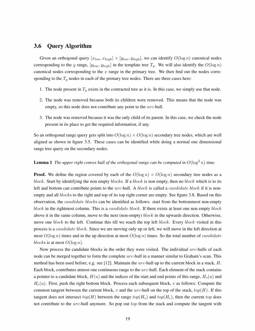
Given an orthogonal query [xlow, xhigh] × [ylow, yhigh], we can identify O(log n) canonical nodescorresponding to the y range, [ylow, yhigh] in the template tree Ty. We will also identify the O(log n)

canonical nodes corresponding to the x range in the primary tree. We then find out the nodes corre-sponding to the Ty nodes in each of the primary tree nodes. There are three cases here:

1. The node present in Ty exists in the contracted tree as it is. In this case, we simply use that node.

2. The node was removed because both its children were removed. This means that the node wasempty, so this node does not contribute any point to the urc-hull.

3. The node was removed because it was the only child of its parent. In this case, we check the nodepresent in its place to get the required information, if any.

So an orthogonal range query gets split into O(log n)×O(log n) secondary tree nodes, which are wellaligned as shown in figure 3.5. These cases can be identified while doing a normal one dimensionalrange tree query on the secondary nodes.

Lemma 1 The upper right convex hull of the orthogonal range can be computed in O(log2 n) time.

Proof. We define the region covered by each of the O(log n) × O(log n) secondary tree nodes as ablock. Start by identifying the non empty blocks. If a block is non empty, then no block which is to itsleft and bottom can contribute points to the urc-hull. A block is called a candidate block if it is non-empty and all blocks to the right and top of its top right corner are empty. See figure 3.8. Based on thisobservation, the candidate blocks can be identified as follows: start from the bottommost non-emptyblock in the rightmost column. This is a candidate block. If there exists at least one non empty block

above it in the same column, move to the next (non-empty) block in the upwards direction. Otherwise,move one block to the left. Continue this till we reach the top left block. Every block visited in thisprocess is a candidate block. Since we are moving only up or left, we will move in the left direction atmost O(log n) times and in the up direction at most O(log n) times. So the total number of candidateblocks is at most O(log n).

Now process the candidate blocks in the order they were visited. The individual urc-hulls of eachnode can be merged together to form the complete urc-hull in a manner similar to Graham’s scan. Thismethod has been used before, e.g. see [12]. Maintain the urc-hull up to the current block in a stack, H .Each block, contributes atmost one continuous range to the urc-hull. Each element of the stack containsa pointer to a candidate block, H(u) and the indices of the start and end points of this range, Hs(u) andHe(u). First, push the right bottom block. Process each subsequent block, v as follows: Compute thecommon tangent between the current block, v and the urc-hull on the top of the stack, top(H). If thistangent does not intersect top(H) between the range top(Hs) and top(He), then the current top doesnot contribute to the urc-hull anymore. So pop out top from the stack and compute the tangent with

19

Figure 3.8 Example of a query. The candidate blocks have been darkened.

the new top of the stack. Continue this till the top of the stack is not popped out. Now push the currentblock to the top of the stack and update the ranges appropriately based on the tangent information.

The time taken is mostly for computing the tangents. This has to be done exactly once for eachtime a urc-hull is pushed or popped. Each tangent computation using the method of Overmars and vanLeeuwen [21] takes O(log n) time. This method compares a point on each of the hulls and discardseither the portion before it or the portion after it in the corresponding hull. This is where we use theneighbors of the bridges stored in each secondary tree node. This tangent computation is done O(log n)

times. So the overall time complexity is O(log2 n). �

The above merging algorithm returns a stack of the secondary tree nodes and the indices of the rangethat each of these nodes contribute to the urc-hull. The line segment connecting the end points of twoadjacent nodes in this stack gives the bridge connecting them. Using this structure, we can report all thepoints on the urc-hull in O(log n + h) time as shown in algorithm 1.

3.6.1 Other Problems

We now explain how to solve the extreme point query, line stabbing query and tangent query prob-lems using the stack obtained above without constructing the entire convex hull. Recall that the convexhull was divided into four parts based on the extreme points. For the problems discussed in this section,the answer could be in any of these four parts. It is easy to identify the exact part(s) by comparing theextreme points with the query parameter.

The basic idea is the following: By comparing an edge of the hull with a query parameter, we candiscard, in constant time, either the part before the edge or the part after the edge. We proceed as

20

Input: Tree node u, Indices i and jOutput: Points on the urc-hull corresponding to u from indices i to j, inclusiveif u is a leaf node then

Report the point if i = j = 1else

if Indexl(u) > i thenReport points in the range of the left subtree which forms part of the range [i, j] in theparent hull

endif i ≤ Indexl(u) ≤ j then

Report Bl(u)endif i ≤ Indexl(u) + 1 ≤ j then

Report Br(u)endif Indexl(u) + 1 < j then

Report points in the range of the right subtree which forms part of the range [i, j] in theparent hull

endend

Algorithm 1: Algorithm to report the points on the urc-hull of a node from given indices i to j,inclusive

follows: Compare each bridge connecting adjacent elements in the stack with the query parameter. Ifthe required output lies on one of the bridges, then we report the answer and stop. Otherwise, this willhelp in identifying the exact node which contains the required output. This takes time proportional tothe number of bridges, which is O(log n). Once the node is identified, by comparing the bridge at theroot of the node with the query parameter, we can decide whether we should take the root, or go to theleft or right subtree. This takes time proportional to the height of the tree which is also O(log n). So theoverall time taken is O(log n).

For line stabbing query, there are at most two points to be reported. We have to query for each ofthem separately. Otherwise, it will not be possible to discard a half at each stage in the above algorithm.

3.7 Summary

We modified the structure of a two dimensional range tree such that a query is divided into a grid-like structure. This enables us to prune off a large section while computing the planar convex hull in anorthogonal range query. Thus, we were able to improve the current bounds for the problem.

21

Chapter 4

Generalized Maxima Range Queries

4.1 Introduction

Recall that a point (x, y) is said to dominate another point (x′, y′) if x > x′ and y > y′. We assumethe points are distinct. The maxima of a point set is the subset of points which are not dominated by anyother points. Here, we study a generalized version of orthogonal range maxima queries.

Consider a set of points, S, on a plane where each point has a color associated with it. The color canbe encoded as an integer from 1 to n, where n = |S|. The colors are not necessarily distinct, so eachcolor may occur more than once. We are interested in preprocessing them such that, given an orthogonalrange query, we would like to obtain color wise information about the maxima points. More precisely,given an orthogonal query, q = [xlow, xhigh] × [ylow, yhigh], we would like to report the following: Foreach color c, present in the maxima of P ∩ q, report the number of points having color c and the leftmost point of each such color. The problem is referred to as generalized or colored maxima rangequery reporting.

Let k be the number of colors on the maxima to be reported. Our answer has size O(k), so to beoutput sensitive, we would like our output to take time, which is polynomial in k and log n, but notpolynomial in n. This rules out any method which computes all points on the maxima and then doessome computation on them.

4.2 Applications

Consider the following scenario: We have a list of products, each of which has a set of parameterssuch as price, quality, etc. Each product also belongs to a particular brand. Suppose there are a pairof products such that one is better than the other in all these parameters, i.e. it has lower price, betterquality, etc. In such a case, we will not be interested in the inferior product. This corresponds to a point”dominating” another point. If we discard all such inferior products, we will be left with the ”maximapoints” of the data set. Instead of having different brands, these could be different types of products,e.g. while searching for a neighborhood, these could correspond to schools, shops, restaurants, etc.

22

Instead, of doing the operation on the entire data set, if we are interested only in a particular subsetof products, chosen based on a range of values for the parameters, then we are doing an orthogonalrange query. If we consider the brands as colors, our problem translates to finding the brands whichhave products in such a range query which are not considered inferior as described above.

This is a direct application of the problem discussed in this paper. However, convex hull and rangequeries come often in many data structure related problems, so this problem could appear as sub prob-lems in many other fields.

4.3 Previous Work

Overmars et al. in [21] solved the problem of maintaining the maxima points of dynamic set ofpoints, allowing O(log2 n) time insertions and deletions. The data structure could also report one ortwo sided range queries. Kalavagattu et al. [19] worked on the three and four sided query version of theproblem on a static set of points. For reporting, they use a data structure which stores, for each point,the next point in the range maxima for a three sided query. The first point of the answer is obtainedby using a persistant sorted set data structure. The solution is expanded to four sided queries using anadditional range tree that uses the three sided data structure at each node.

For counting, they maintain a data structure that can answer queries of the form: given a point p, arange q and k < n, if the maxima points of q are sorted by x coordinates, then report the point that is atdistance k from p. Using this data structure, the number of points in the maxima of a query range can befound using binary search. Similar to reporting, four sided queries are solved using an additional rangetree.

Brodal et al. [8] solved the dynamic version of the same problem, using partially persistent priorityqueues. Rahul et. al. [22] solved a similar problem where the range query is on a particular set ofdimensions and the maxima is computed based on a different set of dimensions. The colored version ofmaxima range queries has not been studied before.

4.4 Preliminaries

4.4.1 Generalized Reporting

Consider a set of points in one dimension where each point has a color associated with it, not neces-sarily unique. We want to preprocess them such that given a range query, we want to report the numberof distinct colors in that range.

Gupta et al. gave a solution in [16] for this problem which takes O(log n + k) to report k points.We describe this method briefly as this will be extensively used in the coming sections. Let P ={p1, p2, ...pl} be a static set of l sorted points along a line, where each point has a color between 1

and l, not necessarily distinct, associated with it. Let pred(pi) be the closest point to pi on its left which

23

is of the same color. pred value of the left most point of each color is set to −∞. Map each point pito the point (pi, pred(pi)) on a plane. Given a range query q = [xl, xh], we want to find the left mostpoint of each color which lies in this range. Let (x′, y′) be one such point. We want x′ to be in the range[xl, xh] and y′ to be such that it is less than xl. Otherwise, this point will not the left most point of thiscolor. So the problem reduces to finding all points in the orthogonal range [xl, xh] × (−∞, xl]. Thisis the three sided orthogonal range reporting problem in two dimensions and can be solved using thepriority search tree data structure. The points will be reported in the sorted order of their x coordinates.Constructing the priority search tree takes O(n log n) time and it takes O(n) space. Computing thepred values can also be done in the same preprocessing time and space complexity.

4.4.2 Heavy Light Decomposition

Let D be a data structure which supports range query operations on a static set of points in onedimension. Heavy light decomposition is a technique to support the same operations on path queries ona tree using the data structure D. More formally, let P be a static set of sorted points along a line. D

is a data structure which supports the following kind of queries: given a query q = [xl, xh], compute afunction f with respect to all points in P ∩q. Now, let T be a static tree. After preprocessing with heavylight decomposition, given a query u, v, where u and v are vertices in T , we can compute f with respectto all points on the path from u to v in the tree T . The function f should satisfy the decomposabilityproperty, i.e., given two disjoint sets, S1 and S2, we should be able to compute f(S1 ∪ S2) from f(S1)

and f(S2), e.g., computing the maximum of a set of numbers is decomposable, while computing thestandard deviation is non-decomposable.

4.4.2.1 Preprocessing

Let size(u) be the number of vertices in the subtree rooted at u. An edge is classified as heavy ifsize(u) > 1

2size(parent(u)). Otherwise, the edge is considered light. The following properties canbe shown easily

1. Among the edges which go from a node to its children, only one can be heavy.

2. Each connected set of heavy edges form a path.

3. A path between any pair of nodes u and v can be expressed as a concatenation of O(log n) lightedges and O(log n) heavy paths.

During preprocessing stage, we do the preprocessing of the linear data structure on all the individualheavy edge paths. Each node takes only O(1) space to store the extra information. Therefore, thepreprocessing time and space is the same as that of the underlying data structure.

24

4.4.2.2 Query

Given a query {u, v}, we can identify the heavy paths and the light edges by traversing the treeappropriately. After this, for the heavy paths, we do a range query on the one dimensional data structure.Using these values along with the values of the light edges, we can compute the function f for the pathfrom u to v.

4.5 Generalized Maxima Queries

Due to the nature of information conveyed by the maximal chain of a set of points, it is common toperform orthogonal range queries that are unbounded in one or two directions. We present solutions tothree representative types of range queries for the maxima problem.

4.5.1 Two Sided Queries

We begin with the simplest kind of maxima queries, where the query range is unbounded in twodirections. We solve for query ranges of the type [xl,∞) × [yl,∞). Notice that in such queries, therange maxima is nothing but a continuous subset of the maximal chain of the entire point-set. Thereforefor this type of two-sided query, reporting the generalized range maxima is equivalent to the generalizedreporting problem in one dimension. This can be solved using the method described in Section 4.4.1.The remaining three types of two-sided queries, however, cannot be solved using this approach.

Theorem 2 Let P be a set of colored points in two dimensions. P can be preprocessed into a O(n)

space and O(n log n) preprocessing time data structure such that given a two-sided query q unbounded

in the positive x and positive y directions, the c distinct colors in the maxima of P ∩ q can be reported

in O(log n + c) time.

4.5.2 Three Sided Queries

In a three sided query, the maximal chain need not be a continuous subset of the maximal chain forthe entire point set. We solve the problem for three sided queries unbounded in the positive x direction,i.e. queries of the type [xl,∞) × [yl, yh], where yl < yh. The solution is similar to that of Kalavagattuin et al. [19].

We construct a one dimensional range tree on the x co-ordinates of the points in P . Let us call thistree Tx. Let S(v) be the subtree of an internal node v in Tx. At each internal node v, we store a pointerto the point in S(v) having the maximum y co-ordinate.

For a point p = (px, py), let nextp(p) be the point with maximum y co-ordinate in its south-eastquadrant, i.e. in the range [px,∞)× (−∞, py]. We construct a graph where each point in P is a vertexand there is an edge from each pi to nextp(pi). We create a dummy vertex pnull. For all such points pi

25

for which no nextp(pi) value exists in P , we add an edge (pi, pnull) to the graph. The nextp(.) valuescan be computed in O(n log n) time using the tree Tx described above. Each vertex in this graph, exceptpnull has exactly one outgoing edge (edge pointing towards its nextp(.) point) and there are no cycles.Therefore, this graph is a tree. We call it T . A maximal chain, as reported by a three sided query, willbe a path in T .

We now decompose T using heavy-light decomposition. We preprocess all heavy paths with the datastructure D of Section 4.4.1. For light edges we do not perform any preprocessing.

Theorem 3 Let P be a set of colored points in two dimensions. P can be processed into a O(n) space

and O(n log n) preprocessing time data structure such that given a three sided query q, unbounded on

the right, the c distinct colors in the maxima of P ∩ q can be reported in O(log2 n + c log n) time per

query.

Proof. The preprocessing stage involves:

1. The building of the tree Tx, which is a one dimensional range tree. It takes O(n) space and canbe built in O(n log n) time.

2. The building of the tree T , which takes O(n log n) time. The number of nodes in T is the sameas the number of points in P , therefore T has size O(n). In addition, for each heavy path in T webuild the data structure D of section 4.4.1. If the length of a heavy path is lh, it takes O(lh) spaceand O(lh log lh) time to build the required data structure. Clearly the overall space requirement isO(n) while the time required is O(n log n).

Thus, for preprocessing, the total space requirement is O(n) and the total time required is O(n log n).Given a query [xl,∞)× [yl, yh], let pa ∈ P be the point with the maximum y co-ordinate lying in the

range [xl,∞)× [−∞, yh]. This point can be found in O(log n) time by an orthogonal range successorquery on the tree Tx. The point pa will be one end point of the maximal chain in P ∩ q. Let pb be theother end point and Pmc be the path in T from pa to pb. It can be shown that pb will be an ancestor of pain the tree T . Therefore, it follows from Section 4.4.2 that the path Pmc will consist of O(log n) lightedges and O(log n) heavy paths.

For heavy paths, we can report the distinct colors using the preprocessed data structure D of Section4.4.1. This takes O(log n+ c) time per heavy path. Since there are O(log n) heavy paths, the total timerequired is O(log2 n + c log n) For the remaining points, i.e. those that are not part of a heavy path, wesimply report the colors when such a point is encountered. This takes a total of O(log n) time sincethere are O(log n) light edges. Thus reporting the colors on the maximal chain for a three sided querycan be done in O(log2 n + c log n). However, there still remains the issue of duplicates.

To ensure that each color in the maxima is reported only once, we leverage the fact that colors areencoded as integers from 1 to C. For every query we initialize a bit-array B, of size C, with all B[i] setto 0. As colors are reported from T , for every reported color k we check the value of B[k]. If B[k] = 0,

26

we output color k and set B[k] to 1, else we do not output color k and move on. Since there are a total ofO(c) colors output by T , the aggregation process will not be a dominating factor in the query time. �

4.5.3 Four Sided Query

Four sided (rectangular) orthogonal range queries can be answered using a range tree together withthe structure for three sided queries (Section 4.5.2).

Theorem 4 Let P be a set of colored points in two dimensions. P can be processed into a O(n log n)

space and O(n log2 n) preprocessing time data structure such that given a four sided query q, the c

distinct colors in the maxima of P ∩ q can be reported in O(log3 n + c log2 n) time per query.

Proof. Let Tx be a one dimensional range tree on the x co-ordinates of all points in P . Let S(v) bethe subtree of an internal node v in Tx. At each internal node v, we populate the structures described inSection 4.5.2 for three sided queries, using the points in S(v) as the input. This takes O(|S(v)|) spaceand O(|S(v)| log |S(v)|) time per internal node v.

Now consider the set Sd of all nodes lying at depth d in the primary tree Tx. The total time requiredto preprocess all nodes in Sd will be:∑

v∈Sd

O(|S(v)| log |S(v)|) ≤∑v∈Sd

O(|S(v)| log n) = O(log n∑v∈Sd

|S(v)|) = O(n log n) (4.1)

Likewise, the total space required to store the preprocessed data structures on each node in Sd will be:∑v∈Sd

O(|S(v)|) = O(∑v∈Sd

|S(v)|) = O(n) (4.2)

There will be O(log n) levels in the tree Tx. From equations (4.1) and (4.2) it follows that preprocessingthe entire tree will take O(n log2 n) time and O(n log n) space.

Given a query q = [xl, xh]× [yl, yh], we first query Tx with the range [xl, xh]. This gives us O(log n)

canonical nodes. We process these canonical nodes from right to left, starting with the canonical nodewhose x range has upper boundary xh. On the first canonical node, we do a three sided query [xl,∞]×[yl, yh]. Let ym be the y co-ordinate of the point with maximum y on the maximal chain of the pointscovered by this canonical node. Points whose y co-ordinate is less than ym in the remaining canonicalnodes cannot lie on the maximal chain of the query region. So on the next canonical node, we do athree sided query [xm,∞]× [ym, yh], and so on. Each of these queries will return at most c colors. Thetime taken per canonical node will be O(log2 n + c log n). Since there are O(log n) canonical nodes,the total time per query will be O(log3 n + c log2 n). Note that even though the colors output by eachcanonical node will be distinct within themselves, the overall set may have duplicates. To remove them,we will once again use the bit array method described in the proof of Theorem 3. �

27

4.6 Summary

The main problem solved in this paper was the reporting of distinct colors present in the maximaof a range query in an output sensitive manner. We first gave a data structure for solving the rangemaxima problem which can be represented as a tree. We used heavy light decomposition on this tree tohelp in performing range queries on them. To support generalized queries, we used the transformationtechnique. Combining all these, we were able to solve the generalized maxima range reporting problem.

The problem of counting the number of such distinct colors in time independent of c remains open.Solving this problem for a dynamic set of problems is also interesting.

28

Chapter 5

Conclusions

In this thesis, we introduced various range query problems and provided efficient data structures tosolve them. We now summarize our results.

Table 5.1 Summary of our resultsProblem Existing Solution Our Solution

(Query Time and Space Usage) (Query Time and Space Usage)Planar convex hull O(log5 n + h), O(n log2 n) O(log2 n + h), O(n log n)

Line stabbing, tangent query O(log2 n) for a range, O(log n)and extreme point in a direction O(log5 n), O(n log2 n) for each additional query on that

range queries range , O(n log n) space

Generalized skyline reporting(4 sided) Not studied O(c log2 n + log3 n), O(n log n)

Generalized skyline reporting(3 sided) Not studied O(c log n + log2 n), O(n)

The problems gave rise to a large number of open problems. We now discuss some future workwhich can be done by enhancing our data structures.

1. Use for other data structures: The enhanced multi dimensional range tree can be used to solvevarious other problems. We expect this to improve the bounds on reporting the largest enclosingdisk or the width of the points in a query rectangle.

2. Proving lower bounds: We have not proven any of the bounds given in this thesis as the mostoptimal. It might be possible to improve them. If not, then proving that lower bound is open.

3. Generalized skyline counting: We have not been able to achieve any result for this problem otherthan counting all the points given by the reporting algorithm. Developing an output sensitivealgorithm for this is still open.

29

4. Solving for dynamic points: All algorithms presented here work on a static set of points. Solvingthese problems on a dynamic set of problems is interesting.

5. Solving in higher dimensions: All the data structures we presented work in only two dimensions.The problems are still open in higher dimensions.

Various combinations of the above points give rise to more interesting problems.

30

Bibliography

[1] M. A. Abam, M. de Berg, and B. Speckmann. Kinetic kd-trees and longest-side kd-trees. SIAM J. Comput.,

39(4):1219–1232, 2009.

[2] A. Andrew. Another efficient algorithm for convex hulls in two dimensions. Information Processing Letters,

9(5):216 – 219, 1979.

[3] F. Aurenhammer. Voronoi diagrams - a survey of a fundamental geometric data structure. ACM Comput.

Surv., 23(3):345–405, 1991.

[4] O. Berkman and U. Vishkin. Recursive star-tree parallel data structure. SIAM J. Comput., 22(2):221–242,

1993.

[5] P. Brass, C. Knauer, C. Shin, and M. Smid. Range-aggregate queries for geometric extent problems. In

A. Wirth, editor, Theory of Computing 2013 (CATS 2013), volume 141 of CRPIT, pages 3–10, Adelaide,

Australia, 2013. ACS.

[6] G. S. Brodal and R. Jacob. Dynamic planar convex hull. In FOCS, pages 617–626, 2002.

[7] G. S. Brodal and A. G. Jørgensen. Data structures for range median queries. In ISAAC, pages 822–831,

2009.

[8] G. S. Brodal and K. Tsakalidis. Dynamic planar range maxima queries. In ICALP (1), pages 256–267,

2011.

[9] T. M. Chan. Optimal output-sensitive convex hull algorithms in two and three dimensions. Discrete &

Computational Geometry, 16(4):361–368, 1996.

[10] T. M. Chan. Dynamic planar convex hull operations in near-logarithmaic amortized time. J. ACM, 48(1):1–

12, 2001.

[11] T. M. Chan. Three problems about dynamic convex hulls. In Symposium on Computational Geometry,

pages 27–36, 2011.

[12] T. M. Chan and E. Y. Chen. Multi-pass geometric algorithms. Discrete & Computational Geometry,

37(1):79–102, 2007.

[13] T. M. Chan, S. Durocher, K. G. Larsen, J. Morrison, and B. T. Wilkinson. Linear-space data structures for

range mode query in arrays. In STACS, pages 290–301, 2012.

[14] J. Fischer and V. Heun. A new succinct representation of rmq-information and improvements in the en-

hanced suffix array. In ESCAPE, pages 459–470, 2007.

31

[15] R. L. Graham. An efficient algorithm for determining the convex hull of a finite planar set. Inf. Process.

Lett., 1(4):132–133, 1972.

[16] P. Gupta, R. Janardan, and M. H. M. Smid. Further results on generalized intersection searching problems:

Counting, reporting, and dynamization. In WADS, pages 361–372, 1993.

[17] J. Hershberger and S. Suri. Offline maintenance of planar configurations. In SODA, pages 32–41, 1991.

[18] R. A. Jarvis. On the identification of the convex hull of a finite set of points in the plane. Inf. Process. Lett.,

2(1):18–21, 1973.

[19] A. K. Kalavagattu, J. Agarwal, A. S. Das, and K. Kothapalli. On counting range maxima points in plane. In

IWOCA, pages 263–273, 2012.

[20] D. G. Kirkpatrick and R. Seidel. The ultimate planar convex hull algorithm. SIAM J. Comput., 15(1):287–

299, Feb. 1986.

[21] M. H. Overmars and J. van Leeuwen. Maintenance of configurations in the plane. J. Comput. Syst. Sci.,

23(2):166–204, 1981.

[22] S. Rahul and R. Janardan. Algorithms for range-skyline queries. In SIGSPATIAL/GIS, pages 526–529,

2012.

32