Randomized Shellsort: A Simple Oblivious Sorting...

Randomized Shellsort: A Simple Oblivious Sorting Algorithm

Michael T. GoodrichDept. of Computer Science

University of California, Irvinehttp://www.ics.uci.edu/∼goodrich/

AbstractIn this paper, we describe a randomized Shellsort algorithm.This algorithm is a simple, randomized, data-oblivious ver-sion of the Shellsort algorithm that always runs in O(n log n)time and succeeds in sorting any given input permutationwith very high probability. Taken together, these propertiesimply applications in the design of new efficient privacy-preserving computations based on the secure multi-partycomputation (SMC) paradigm. In addition, by a trivial con-version of this Monte Carlo algorithm to its Las Vegas equiv-alent, one gets the first version of Shellsort with a runningtime that is provably O(n log n) with very high probability.

1 IntroductionJuly 2009 marked the 50th anniversary1 of the Shellsortalgorithm [45]. This well-known sorting algorithm (whichshould always be capitalized, since it is named after itsinventor) is simple to implement. Given a sequence of offsetvalues, (o1, o2, . . . , op), with each oi < n, and an unsortedarray A, whose n elements are indexed from 0 to n − 1, theShellsort algorithm (in its traditional form) is as follows:

for i = 1 to p dofor j = 0 to oi − 1 do

Sort the subarray of A consisting of indicesj, j + oi, j + 2oi, . . ., e.g., using insertion-sort.

In fact, even this traditional version of Shellsort is actu-ally a family of algorithms, since there are so many differentoffset sequences. The trick in implementing a traditional ver-sion of Shellsort, therefore, is coming up with a good offsetsequence. Pratt [36] shows that using a sequence consistingof all products of powers of 2 and 3 less than n results in aworst-case running time of O(n log2 n). Several other offsetsequences have been studied (e.g., see the excellent survey ofSedgewick [42]), but none beat the asymptotic performance

1This paper is dedicated to my parents, Ronald and Grace Goodrich, tocommemorate their 50th wedding anniversary.

of the Pratt sequence. Moreover, Plaxton and Suel [35] es-tablish a lower bound of Ω(n log2 n/(log log n)2) for theworst-case running time of Shellsort with any input sequence(see also [11]) and Jiang et al. [23] establish a lower boundof Ω(pn1+1/p) for the average-case running time of Shell-sort. Thus, the only way to achieve an O(n log n) average-time bound for Shellsort is to use an offset sequence oflength Θ(log n), and, even then, the problem of provingan O(n log n) average running-time bound for a version ofShellsort is a long-standing open problem [42].

The approach we take in this paper is to consider avariant of Shellsort where the offset sequence is a fixedsequence, (o1, o2, . . . , op), of length O(log n)—indeed, wejust use powers of two—but the “jumps” for each offset valuein iteration i are determined from a random permutationbetween two adjacent regions in A of size oi (starting atindices that are multiples of oi). The standard Shellsortalgorithm is equivalent to using the identity permutationbetween such region pairs, so it is appropriate to considerthis to be a randomized variant of Shellsort.

In addition to variations in the offset sequence and howit is used, there are other existing variations to Shellsort,which are based on replacing the insertion-sort in the in-ner loop with other actions. For instance, Dobosiewicz [12]proposes replacing the insertion-sort with a single linear-time bubble-sort pass—doing a left-to-right sequence ofcompare-exchanges between elements at offset-distancesapart—which will work correctly, for example, with the Prattoffset sequence, and which seems to work well in practice forgeometric offset sequences with ratios less than 1.33 [12].Incerpi and Sedgewick [21, 22] study a version of Shell-sort that replaces the insertion-sort by a shaker pass (seealso [7, 46]). This is a left-to-right bubble-sort pass fol-lowed by a right-to-left bubble-sort pass and it also seemsto do better in practice for geometric offset sequences [22].Yet another modification of Shellsort replaces the insertion-sort with a brick pass, which is a sequence of odd-evencompare-exchanges followed by a sequence of even-oddcompare-exchanges [42]. While these variants perform wellin practice, we are not aware of any average-case analysisfor any of these variants of Shellsort that proves they have

1262 Copyright © by SIAM. Unauthorized reproduction of this article is prohibited.

an expected running time of O(n log n). Sanders and Fleis-cher [39] describe an algorithm they call “randomized Shell-sort,” which is a data-dependent Shellsort algorithm as in theabove pseudo-code description, except that it uses productsof random numbers as its offset sequence. They don’t provean O(n log n) average-time bound for this version, but theydo provide some promising empirical data to support an av-erage running time near O(n log n); see also [31].

1.1 Data-Oblivious SortingIn addition to its simplicity, one of the interesting propertiesof Shellsort is that many of its variants are data-oblivious.Specifically, if we view compare-exchange operations as aprimitive (i.e., as a “black box”), then Shellsort algorithmswith bubble-sort passes, shaker passes, brick passes, orany combination of such sequences of data-independentcompare-exchange operations, will perform no operationsthat depend on the relative order of the elements in theinput array. Such data-oblivious algorithms have severaladvantages, as we discuss below.

Data-oblivious sorting algorithms can also be viewed assorting networks [25], where the elements in the input arrayare provided as values given on n input wires and internalgates are compare-exchanges. Ajtai, Komlos, and Szemeredi(AKS) [1] show that one can achieve a sorting networkwith O(n log n) compare-exchange gates in the worst case,but their method is quite complicated and has a very largeconstant factor, even with subsequent improvements [34,43]. Leighton and Plaxton [27] describe a randomizedmethod for building a data-oblivious sorting network thatuses O(n log n) compare-exchange gates and sorts any giveninput array with very high probability. Unfortunately, eventhough the Leighton-Plaxton sorting algorithm is simplerthan the AKS sorting network, it is nonetheless consideredby some not to be simple in an absolute sense (e.g., see [42]).

One can also simulate other parallel sorting algorithmsor network routing methods, but these don’t lead to simpletime-optimal data-oblivious sequential sorting algorithms.For example, the online routing method of Arora et al. [2]is time-optimal but not data-oblivious, as are the PRAMsorting algorithms of Shavit et al. [44], Cole [9], Reif [38],and Goodrich and Kosaraju [18]. The shear-sort algorithm ofScherson and Sen [40] is simple and data-oblivious but nottime-optimal. The columnsort algorithm of Leighton [26]and the sorting method of Maggs and Vocking [28] areasymptotically fast, but they both employ the AKS network;hence, they are not simple.

Finally, note that well-known time-optimal sorting algo-rithms, such as radix-sort, quicksort, heapsort, and mergesort(e.g., see [10,16,19,41]), are not data-oblivious. In addition,well-known data-oblivious sorting algorithms, such as odd-even mergesort and Batcher’s bitonic sort (e.g., see [25]), as

well as Pratt’s version of Shellsort [36], run in Θ(n log2 n)time. Therefore, existing sorting algorithms arguably do notprovide a simple data-oblivious sorting algorithm that runsin O(n log n) time and succeeds with very high probabilityfor any given input permutation.

Modern Motivations for Simple Data-Oblivious Sorting.Originally, data-oblivious sorting algorithms were motivatedprimarily from their ability to be implemented in special-purpose hardware modules [24]. Interestingly, however,there is a new, developing set of applications for data-oblivious sorting algorithms in information security andprivacy.

In secure multi-party computation (SMC) protocols(e.g., see [5, 8, 13, 14, 29, 30]), two or more parties sep-arately hold different portions of a collection of data val-ues, x1, x2, . . . , xn, and are interested in computing somefunction, f(x1, x2, . . . , xn), on these values. In addition,due to privacy concerns, none of the different parties is will-ing to reveal the specific values of his or her pieces of data.SMC protocols allow the parties to compute the value of fon their collective input values without revealing any of theirspecific data values (other than what can inferred from theoutput function, f , itself [17]).

One of the main tools for building SMC protocols isto encode the function f as a circuit and then simulatean evaluation of this circuit using digitally-masked values,as in the Fairplay system [5, 29]. By then unmaskingonly the output value(s), the different parties can learnthe value of f without revealing any of their own datavalues. Unfortunately, from a practical standpoint, SMCsystems like Fairplay suffer from a major efficiency problem,since encoding entire computations as circuits can involvesignificant blow-ups in space (and simulation time). Theseblow-ups can be managed more efficiently, however, byusing data-oblivious algorithms to drive SMC computationswhere only the primitive operations (such as MIN, MAX,AND, ADD, or compare-exchange) are implemented assimulated circuits. That is, each time such an operation isencountered in such a computation, the parties perform anSMC computation to compute its masked value, with therest of the steps of the algorithm performed in an obliviousway. Thus, for a problem like sorting, which in turn canbe used to generate random permutations, in a privacy-preserving way, being able to implement the high-level logicin a data-oblivious manner implies that simulating onlythe low-level primitives using SMC protocols will revealno additional information about the input values. Thiszero-additional-knowledge condition follows from the factthat data-oblivious algorithms use their low-level primitiveoperations in ways that don’t depend on input data values.Therefore, we would like to have a simple data-oblivioussorting algorithm, so as to drive efficient SMC protocols thatuse sorting as a subroutine.


1.2 Our ResultsIn this paper, we present a simple, data-oblivious randomizedversion of Shellsort, which always runs in O(n log n) timeand sorts with very high probability. In particular, theprobability that it fails to sort any given input permutationwill be shown to be at most 1/nb, for constant b ≥ 1, whichis the standard for “very high probability” (v.h.p.) that weuse throughout this paper.

Although this algorithm is quite simple, our analysisthat it succeeds with very high probability is not. Our proofof probabilistic correctness uses a number of different tech-niques, including iterated Chernoff bounds, the method ofbounded average differences for Doob martingales, and aprobabilistic version of the zero-one principle. Our analysisalso depends on insights into how this randomized Shellsortmethod brings an input permutation into sorted order, includ-ing a characterization of the sortedness of the sequence interms of “zones of order.” We bound the degree of zero-oneunsortedness, or dirtiness, using three probabilistic lemmasand an inductive argument showing that the dirtiness dis-tribution during the execution of our randomized Shellsortalgorithm has exponential tails with polylogarithmic dirti-ness at their ends, with very high probability (w.v.h.p.). Weestablish the necessary claims by showing that the regioncompare-exchange operation simultaneously provides threedifferent kinds of near-sortedness, which we refer to as a“leveraged-splitters.” We show that, as the algorithm pro-gresses, these leveraged-splitters cause the dirtiness of thecentral region, where zeroes and ones meet, to become pro-gressively cleaner, while the rest of the array remains veryclean, so that, in the end, the array becomes sorted, w.v.h.p.

In addition to this theoretical analysis, we also providea Java implementation of our algorithm, together with someexperimental results.

As a data-oblivious algorithm, our randomized Shellsortmethod is a Monte Carlo algorithm (e.g., see [32,33]), in thatit always runs in the same amount of time but can sometimesfail to sort. It can easily be converted into a data-dependentLas Vegas algorithm, however, which always succeeds buthas a randomized running time, by testing if its output issorted and repeating the algorithm if it is not. Such a data-dependent version of randomized Shellsort would run inO(n log n) time with very high probability; hence, it wouldprovide the first version of Shellsort that provably runs inO(n log n) time with very high probability.

2 Randomized ShellsortIn this section, we describe our randomized Shellsort algo-rithm. As we show in the sections that follow, this algorithmalways runs in O(n log n) time and is highly likely to suc-ceed in sorting any given input permutation.

Suppose that we are given an n-element array, A, that

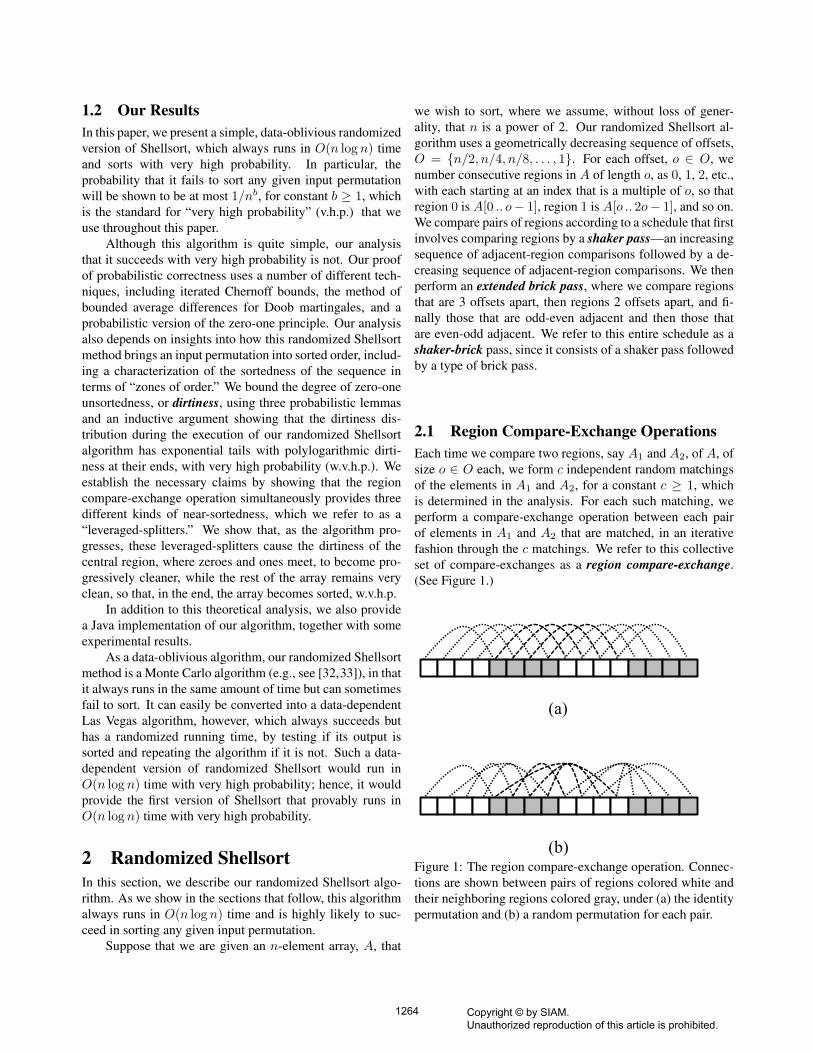
we wish to sort, where we assume, without loss of gener-ality, that n is a power of 2. Our randomized Shellsort al-gorithm uses a geometrically decreasing sequence of offsets,O = n/2, n/4, n/8, . . . , 1. For each offset, o ∈ O, wenumber consecutive regions in A of length o, as 0, 1, 2, etc.,with each starting at an index that is a multiple of o, so thatregion 0 is A[0 .. o− 1], region 1 is A[o .. 2o− 1], and so on.We compare pairs of regions according to a schedule that firstinvolves comparing regions by a shaker pass—an increasingsequence of adjacent-region comparisons followed by a de-creasing sequence of adjacent-region comparisons. We thenperform an extended brick pass, where we compare regionsthat are 3 offsets apart, then regions 2 offsets apart, and fi-nally those that are odd-even adjacent and then those thatare even-odd adjacent. We refer to this entire schedule as ashaker-brick pass, since it consists of a shaker pass followedby a type of brick pass.

2.1 Region Compare-Exchange OperationsEach time we compare two regions, say A1 and A2, of A, ofsize o ∈ O each, we form c independent random matchingsof the elements in A1 and A2, for a constant c ≥ 1, whichis determined in the analysis. For each such matching, weperform a compare-exchange operation between each pairof elements in A1 and A2 that are matched, in an iterativefashion through the c matchings. We refer to this collectiveset of compare-exchanges as a region compare-exchange.(See Figure 1.)

(a)

(b)Figure 1: The region compare-exchange operation. Connec-tions are shown between pairs of regions colored white andtheir neighboring regions colored gray, under (a) the identitypermutation and (b) a random permutation for each pair.


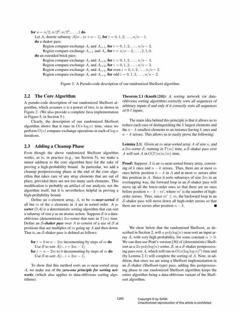
for o = n/2, n/22, n/23, . . . , 1 doLet Ai denote subarray A[io .. io + o− 1], for i = 0, 1, 2, . . . , n/o− 1.do a shaker pass:

Region compare-exchange Ai and Ai+1, for i = 0, 1, 2, . . . , n/o− 2.Region compare-exchange Ai+1 and Ai, for i = n/o− 2, . . . , 2, 1, 0.

do an extended brick pass:Region compare-exchange Ai and Ai+3, for i = 0, 1, 2, . . . , n/o− 4.Region compare-exchange Ai and Ai+2, for i = 0, 1, 2, . . . , n/o− 3.Region compare-exchange Ai and Ai+1, for even i = 0, 1, 2, . . . , n/o− 2.Region compare-exchange Ai and Ai+1, for odd i = 0, 1, 2, . . . , n/o− 2.

Figure 2: A Pseudo-code description of our randomized Shellsort algorithm.

2.2 The Core AlgorithmA pseudo-code description of our randomized Shellsort al-gorithm, which assumes n is a power of two, is as shown inFigure 2. (We also provide a complete Java implementationin Figure 5, in Section 5.)

Clearly, the description of our randomized Shellsortalgorithm shows that it runs in O(n log n) time, since weperform O(n) compare-exchange operations in each of log niterations.

2.3 Adding a Cleanup PhaseEven though the above randomized Shellsort algorithmworks, as is, in practice (e.g., see Section 5), we make aminor addition to the core algorithm here for the sake ofproving a high-probability bound. In particular, we add acleanup postprocessing phase at the end of the core algo-rithm that takes care of any stray elements that are out ofplace, provided there are not too many such elements. Thismodification is probably an artifact of our analysis, not thealgorithm itself, but it is nevertheless helpful in proving ahigh-probability bound.

Define an n-element array, A, to be m-near-sorted ifall but m of the n elements in A are in sorted order. A p-sorter [3, 4] is a deterministic sorting algorithm that can sorta subarray of size p as an atomic action. Suppose S is a data-oblivious (deterministic) 2m-sorter that runs in T (m) time.Define an S-shaker pass over A to consist of a use of S atpositions that are multiples of m going up A and then down.That is, an S-shaker pass is defined as follows:

for i = 0 to n− 2m incrementing by steps of m doUse S to sort A[i .. i + 2m− 1].

for i = n− 2m to 0 decrementing by steps of m doUse S to sort A[i .. i + 2m− 1].

To show that this method sorts an m-near-sorted arrayA, we make use of the zero-one principle for sorting net-works (which also applies to data-oblivious sorting algo-rithms):

Theorem 2.1 (Knuth [24]): A sorting network (or data-oblivious sorting algorithm) correctly sorts all sequences ofarbitrary inputs if and only if it correctly sorts all sequencesof 0-1 inputs.

The main idea behind this principle is that it allows us toreduce each case of distinguishing the k largest elements andthe n−k smallest elements to an instance having k ones andn− k zeroes. This allows us to easily prove the following:

Lemma 2.1: Given an m-near-sorted array A of size n, anda 2m-sorter S, running in T (m) time, a S-shaker pass overA will sort A in O(T (m)n/m) time.

Proof: Suppose A is an m-near-sorted binary array, consist-ing of k ones and n − k zeroes. Thus, there are at most mones below position n − k in A and at most m zeroes afterthis position in A. Since it sorts subarrays of size 2m in anoverlapping way, the forward loop in an S-shaker pass willmove up all the lower-order ones so that there are no onesbefore position n−k−m′, where m′ is the number of high-order zeroes. Thus, since m′ ≤ m, the backward loop in anS-shaker pass will move down all high-order zeroes so thatthere are no zeroes after position n− k.

We show below that the randomized Shellsort, as de-scribed in Section 2, will α polylog(n)-near-sort an input ar-ray A, with very high probability, for some constant α > 0.We can then use Pratt’s version [36] of (deterministic) Shell-sort as a 2α polylog(n)-sorter, S, in a S-shaker postprocess-ing pass over A, which will run in O(n(log log n)2) time and(by Lemma 2.1) will complete the sorting of A. Note, in ad-dition, that since we are using a Shellsort implementation inan S-shaker (Shellsort-type) pass, adding this postprocess-ing phase to our randomized Shellsort algorithm keeps theentire algorithm being a data-oblivious variant of the Shell-sort algorithm.


3 Analyzing the Region Compare-Exchange Operations

Let us now turn to the analysis of the ways in which regioncompare-exchange operations bring two regions in our size-n input array closer to a near-sorted order. We begin with adefinition.

3.1 Leveraged SplittersAjtai, Komlos, and Szemeredi [1] define a λ-halver of asequence of 2N elements to be an operation that, for any k ≤N , results in a sequence so that at most λk of the largest kelements from the sequence are in the first k positions, and atmost λk of the smallest k elements are in the last k positions.We define a related notion of a (µ, α, β)-leveraged-splitter tobe an operation such that, for the k ≤ (1−ε)N largest (resp.,smallest) elements, where 0 ≤ ε < 1, the operation returns asequence with at most

maxα(1− ε)µN, β

of the k largest (smallest) elements on the left (right)half. Thus, a λ-halver is automatically a (1, λ, 0)-leveraged-splitter, but the reverse implication is not necessarily true.The primary advantage of the leveraged-splitter conceptis that it captures the way that c random matchings withcompare-exchanges has a modest impact with respect to aroughly equal number of largest and smallest elements, butthey have a geometric impact with respect to an imbalancednumber of largest and smallest elements. We show belowthat a region compare-exchange operation consisting of atleast c ≥ 3 random matchings is, with very high probability,a (α, β, µ)-leveraged-splitter for each of the following setsof parameters:• µ = c + 1, α = 1/2, and β = 0,• µ = c + 1, α = (2e)c, and β = 4e log n,• µ = 0, α = 1/6, and β = 0.

The fact that the single region compare-exchange operationis a (µ, α, β)-leveraged-splitter for each of these differentsets of parameters, µ, α, and β, allows us to reason aboutvastly divergent degrees of sortedness of the different areasin our array as the algorithm progresses. For instance, weuse the following lemma to reason about regions whosesortedness we wish to characterize in terms of a roughlyequal numbers of smallest and largest elements.

Lemma 3.1: Suppose a (0, λ, 0)-leveraged-splitter is ap-plied to a sequence of 2N elements, and let (1− ε)N ≤ k ≤(1 + ε)N and l = 2N − k, where 0 < λ < 1 and 0 ≤ ε < 1.Then at most (λ + ε)N of the k largest elements end up inthe left half of the sequence and at most (λ + ε)N of the lsmallest elements end up in the right half of the sequence.

Proof: Let us consider the k largest elements, such that(1 − ε)N ≤ k ≤ N . After applying a (0, λ, 0)-leveraged-splitter, there are at at most λN of the k largest elements onthe left half of the sequence (under this assumption about k).Then there are at least N − λN of the l smallest elementson the left left; hence, at most l − (N − λN) of the lsmallest elements on the right half. Therefore, there are atmost N + εN − (N − λN) = (λ + ε)N of the l smallestelements on the right half. A similar argument applies to thecase when N ≤ k ≤ (1 + ε)N to establish an upper boundof at most (λ + ε)N of the k smallest elements on the lefthalf.

Let us know turn to the proofs that region compare-exchange operations are (µ, α, β)-leveraged-splitters, foreach of the sets of parameters listed above.

3.2 The (c + 1, 1/2, 0)-Leveraged-SplitterProperty

We begin with the (c+1, 1/2, 0)-leveraged-splitter property.So suppose A1 and A2 are two regions of size N each thatare being processed in a region compare-exchange operationconsisting of c random matchings. We wish to show that,for the k ≤ (1− ε)N , largest (resp., smallest) elements, thisoperation returns a sequence such that there are at most

(1− ε)c+1

2N

of the k largest (smallest) elements on the left (right) half.Without loss of generality, let us focus on the k largestelements. Furthermore, let us focus on the case where largestk elements are all ones and the 2N − k smallest elementsare all zeroes, since a region compare-exchange operation isoblivious. That is, if a region compare-exchange operation isa (c + 1, 1/2, 0)-leveraged-slitter in the zero-one case, thenit is a (c + 1, 1/2, 0)-leveraged-slitter in the general case aswell.

Let us model the c repeated random matchings used ina region compare-exchange operation between A1 and A2 asa martingale. For each of the k1 positions that are initiallyholding a one on the left side, A1, of our pair of regions,A1 and A2, prior to c random matchings and compare-exchanges, let us define a set, X , of 0-1 random variables,Xi,j , such that is 1 if and only if the i-th position in A1

originally holding a one is matched with a position in A2

holding a one in the j-th repetition of the region compare-exchange operation. Define a failure-counting function, f ,as follows:

f(X1,1, . . . , Xk1,c) =k1∑

i=1

c∏j=1

Xi,j .


That is, f counts the number of ones in A1 that stay in A1

even after c applications of the region compare-exchangeoperation.

Unfortunately, even though the random variables Xi,1,Xi,2, . . ., Xi,c are independent, most other groups of randomvariables in X are not. So we cannot directly apply aChernoff bound (e.g., see [32,33]) to probabilistically boundthe degree to which f differs from its expectation. Wecan nevertheless derive such a bound using the method ofbounded average differences [15].

Imagine that we are computing f incrementally as theXi,j are revealed by an algorithm performing the c regioncompare-exchange operations. Suppose further that theXi,j’s are revealed lexicographically by (i, j) pairs. Thus, fis initially 0 and it increases in value by 1 each time the lastin a set of variables, Xi,1, Xi,2, . . . , Xi,c, is revealed andall the variables in this set equal 1. Note also that during thisprocess, if any Xi,j is 0, then the contribution to f of the i-thone originally in A1 will ultimately be 0. Note, in addition,for each j, that the Xi,j variables are essentially representingour performing a sampling without replacement from amongthe positions on the right side. That is, revealing an Xi,j to be0 potentially removes the chance that the i-th original one inA1 will fail (if it hasn’t already succeeded), while it increasesby at most 1 the remaining expected value for the k1 − iremaining variables in this iteration. Likewise, revealingan Xi,j to be 1 potentially continues the chance that the i-th item will fail (if it hasn’t already succeeded), while itreduces by at most 1 the remaining expected value for thek1 − i remaining variables in this iteration. Thus, giventhe previous choices for the random variables, revealing thevariable Xi,j will either keep f unchanged or increase it byat most 1. Thus, if we let Xi,j denote the random variableassignments prior to the revelation of Xi,j , then we seethat f satisfies a bounded average differences (Lipschitz)condition,

|E(f | Xi,j , Xi,j = 0)− E(f | Xi,j , Xi,j = 1)| ≤ 1.

Therefore, by the method of bounded average differ-ences [15], which is an application of Azuma’s inequalityapplied to the Doob martingale of the above conditional ex-pected values (e.g., see [32, 33]), for t > 0,

Pr(f > E(f) + t) ≤ exp(−t2

2k1

),(3.1)

assuming k1 > 0 (otherwise, f = 0), where k1 is the originalnumber of ones in A1. Note that if the two regions, A1

and A2, being compared are each of size N , c = 1, andk ≤ N is the total number of ones in the two regions, thenE(f) = k1 (k − k1/N). It is not as easy to calculate E(f)for c > 1, but we can often upper bound E(f) by some value

M(N), when c > 1, in which case Equation (3.1) implies

Pr(f > M(N) + t) ≤ exp(−t2

2k1

).(3.2)

Lemma 3.2: Suppose we are given two regions, A1 and A2,each of size N , and let k = k1+k2, where k1 (resp., k2) is thenumber of ones in A1 (resp., A2). Let k

(1)1 be the number of

ones in A1 after a single region compare-exchange matching.Then

E(k(1)1 ) = k1

(k2

N

).

Proof: In order for a one to remain on the left side after aregion compare-exchange matching, it must be matched witha one on the right side. The probability that a one on the leftis matched with a one on the right is k2/N .

For example, we use the above method in the proof ofthe following lemma.

Lemma 3.3 (Fast-Depletion Lemma): Given two binaryregions, A1 and A2, each of size N , let k = k1 + k2, wherek1 and k2 are the respective number of ones in A1 and A2,and suppose k ≤ (1 − ε)N , for 0 ≤ ε < 1. Let k

(c)1 be

the number of ones in A1 after c random matchings (withcompare-exchanges) in a region compare-exchange opera-tion. Then

Pr(

k(c)1 >

(1− ε)c+1N

2

)≤ e−(1−ε)2c+1N/24

.

Proof: In order for a one to stay on the left side, it mustbe matched with a one on the right side in each of the crandom matchings. The probability that it stays on the leftafter the first compare-exchange is [(1− ε)N − k1]/N andthe probability of it staying on the left in each subsequentcompare-exchange is at most 1 − ε. Thus, using the factthat the function, k1[(1 − ε)N − k1], is maximized atk1 = (1− ε)N/2,

E(k

(c)1

)≤ (1− ε)c+1N

22,

which, by Equation (3.2), implies the lemma, using t =(1−ε)c+1N

22 , and the fact that k1 ≤ (1− ε)N .

By a symmetrical argument, we have similar result forthe case of k ≤ (1 − ε)N zeroes that would wind upin A2 after c random matchings (with compare-exchangeoperations between the matched pairs). Thus, we have thefollowing.

Corollary 3.1: If A1 and A2 are two regions of size N each,then a compare-exchange operation consisting of c randommatchings (with compare-exchanges between matched pairs)between A1 and A2 is a (c + 1, 1/2, 0)-leveraged-splitterwith probability at least 1− e−(1−ε)2c+1N/24

.


The above lemma and corollary are most useful for caseswhen the regions are large enough so that the above failureprobability is below O(n−α), for α > 1.

3.3 The (c + 1, (2e)c, 4e log n)-Leveraged-Splitter Property

When region sizes or (1 − ε) values are too small forCorollary 3.1 to hold, we can use the (c+1, (2e)c, 4e log n)-leveraged-splitter property of the region-compare operation.As above, we prove this property by assuming, without lossof generality, that we are operating on a zero-one array andby focusing on the k largest elements, that is, the ones.We also note that this particular (µ, α, β)-leveraged-splitterproperty is only useful when (1 − ε) < 1/(2e), whenconsidering the k ≤ (1 − ε)N largest elements (i.e., theones), so we add this as a condition as well.

Lemma 3.4 (Little-Region Lemma): Given two regions,A1 and A2, each of size N , let k = k1 + k2, where k1 andk2 are the respective number of ones in A1 and A2. Supposek ≤ (1−ε)N , where ε satisfies (1−ε) < 1/(2e). Let k

(c)1 be

the number of ones in A1 after c region compare-exchangeoperations. Then

Pr(k

(c)1 > max(2e)c(1− ε)c+1N, 4e log n

)≤ cn−4.

Proof: Let us apply an induction argument, based onthe number, c′, of random matches in a region compare-exchange operation. Consider an inductive claim, whichstates that after after c′ random matchings (with compare-exchange operations),

k(c′)1 > max(2e)c′

(1− ε)c′+1N , 4e log n,

with probability at most c′n−4. Thus, with high probabilityk

(c′)1 is bounded by the formula on the righthand side. The

claim is clearly true by assumption for c′ = 0. So, supposethe claim is true for c′, and let us consider c′ +1. Since thereis at most a (1− ε) fraction of ones in A2,

µ = E(k(c′+1)1 ) ≤ (2e)c′

(1− ε)c′+2N.

Moreover, the value k(c′+1)1 can be viewed as the number

of ones in a sample without replacement from A2 of sizek

(c′)1 . By an argument of Hoeffding [20], then, the expected

value of any convex function of the size of such a sampleis bounded by the expected value of that function appliedto the size of a similar sample with replacement. Thus, wecan apply a Chernoff bound (e.g., see [32, 33]) to this singlerandom matching and pairwise set of compare-exchangeoperations, to derive

Pr(k

(c′+1)1 > (1 + δ)µ

)< 2−δµ,

provided δ ≥ 2e − 1. Taking (1 + δ)µ = 2eM(N) impliesδ ≥ 2e− 1, where M(N) = (2e)c′

(1− ε)c′+2N ; hence, wecan bound

Pr(k

(c′+1)1 > 2eM(N)

)< 2−(2eM(N)−µ) ≤ 2−eM(N),

which also gives us a new bound on M(N) for the nextstep in the induction. Provided M(N) ≥ 2 log n, then this(failure) condition holds with probability less than n−4. If,on the other hand, M(N) < 2 log n, then

Pr(k

(c′+1)1 > 4e log n

)< 2−(4e log n−µ) ≤ 2−2e log n < n−4.

In this latter case, we can terminate the induction, since re-peated applications of the region compare-exchange opera-tion can only improve things. Otherwise, we continue theinduction. At some point during the induction, we must ei-ther reach c′+1 = c, at which point the inductive hypothesisimplies the lemma, or we will have M(N) < 2 log n, whichputs us into the above second case and implies the lemma.

A similar argument applies to the case of the k smallestelements, which gives us the following.

Corollary 3.2: If A1 and A2 are two regions of size N each,then a compare-exchange operation consisting of c randommatchings (with compare-exchanges between matched pairs)between A1 and A2 is a (c + 1, (2e)c, 4e log n)-leveraged-splitter with probability at least 1− cn−4.

As we noted above, this corollary is only of use for thecase when (1− ε) < 1/(2e), where ε is the same parameteras used in the definition of a (µ, α, β)-leveraged-splitter.

3.4 The (0, 1/6, 0)-Leveraged-Splitter Prop-erty

The final property we prove is for the (0, 1/6, 0)-leveraged-splitter property. As with the other two properties, weconsider here the k largest elements, and focus on the caseof a zero-one array.

Lemma 3.5 (Slow-Depletion Lemma): Given two regions,A1 and A2, each of size N , let k = k1 + k2, where k1

and k2 are the respective number of ones in A1 and A2, andk ≤ N . Let k

(c)1 be the number of ones in A1 after c region

compare-exchange operations. Then k(3)1 ≤ N/6, with very

high probability, provided N is Ω(lnn).

Proof: The proof involves three consecutive applicationsof the method of bounded average differences, with aninterplay of error bounds on k

(1)1 , k

(2)1 , and k

(3)1 , and their

corresponding failure probabilities. As noted above,

E(k

(1)1

)= k1

(1− k1

N

)≤ N

4,


since k1 (1− k1/N) is maximized at k1 = N/2. Thus,applying Equation (3.2), with t = N/27, implies

Pr(

k(1)1 >

(1 +

127

)N

4

)≤ e−N/215

.

So let us assume that k(1)1 is bounded as above. Since

k1 (1− k1/N) is monotonic on [0, N/2],

E(k

(2)1

)≤

(1 +

125

)N

4

(3− 1/25

4

).

Thus, applying Equation (3.2), with t = N/27, implies

Pr(

k(2)1 >

N

5

)≤ e−N/215

,

since (1 +

125

)N

4

(3− 1/25

4

)+

N

27≤ N

5.

So let us assume that k(2)1 ≤ N/5. Thus, since

k1 (1− k1/N) is monotonic on [0, N/2],

E(k

(3)1

)≤ N

5

(1− 1

5

).

Thus, applying Equation (3.2), with t = N/28, and alsousing the fact that k1 ≤ N/5, implies

Pr(

k(3)1 >

N

28+

4N

25

)≤ e−N/216

.

The proof follows from the fact that N/28 + 4N/25 ≤ N/6and that each bound derived on k

(1)1 , k

(2)2 , and k

(3)3 holds

with very high probability.

Of course, the above lemma has an obvious symmetricversions that applies to the number of zeroes on the right sideof two regions in a region compare-exchange. Thus, we havethe following.

Corollary 3.3: If A1 and A2 are two regions of size Neach, then a compare-exchange operation consisting of atleast 3 random matchings (with compare-exchanges be-tween matched pairs) between A1 and A2 is a (0, 1/6, 0)-leveraged-splitter with probability at least 1−cn−4, providedN is Ω(lnn).

4 Analyzing the Core AlgorithmHaving proven the essential properties of a region compare-exchange operation, consisting of c random matchings (withcompare-exchanges between matched pairs), we now turn tothe problem of analyzing the core part of our randomizedShellsort algorithm.

4.1 A Probabilistic Zero-One PrincipleWe begin our analysis with a probabilistic version of thezero-one principle.

Lemma 4.1: If a randomized data-oblivious sorting algo-rithm sorts any binary array of size n with failure probabilityat most ε, then it sorts any arbitrary array of size n with fail-ure probability at most ε(n + 1).

Proof: The lemma2 follows from the proof of Theorem 3.3by Rajasekaran and Sen [37], which itself is based on thejustification of Knuth [24] for the deterministic version ofthe zero-one principle for sorting networks. The essentialfact is that an arbitrary n-element input array, A, has, viamonotonic bijections, at most n + 1 corresponding n-lengthbinary arrays, such that A is sorted correctly by a data-oblivious algorithm, A, if and only if every bijective binaryarray is sorted correctly byA. (See Rajasekaran and Sen [37]or Knuth [24] for the proof of this fact.)

Note that this lemma is only of practical use for ran-domized data-oblivious algorithms that have failure proba-bilities of at most O(n−a), for some constant a > 1. Werefer to such algorithms as succeeding with very high prob-ability. Fortunately, our analysis shows that our randomizedShellsort algorithm will α polylog(n)-near-sort a binary ar-ray with very high probability.

4.2 Bounding Dirtiness after each IterationIn the d-th iteration of our core algorithm, we partition thearray A into 2d regions, A0, A1, . . ., A2d−1, each of sizen/2d. Moreover, each iteration splits a region from theprevious iteration into two equal-sized halves. Thus, thealgorithm can be visualized in terms of a complete binarytree, B, with n leaves. The root of B corresponds to aregion consisting of the entire array A and each leaf of Bcorresponds to an individual cell, ai, in A, of size 1. Eachinternal node v of B at depth d corresponds with a region,Ai, created in the d-th iteration of the algorithm, and thechildren of v are associated with the two regions that Ai issplit into during the (d + 1)-st iteration. (See Figure 3.)

The desired output, of course, is to have each leaf value,ai = 0, for i < n − k, and ai = 1, otherwise. We thereforerefer to the transition from cell n−k− 1 to cell n−k on thelast level of B as the crossover point. We refer to any leaf-level region to the left of the crossover point as a low regionand any leaf-level region to the right of the crossover point asa high region. We say that a region, Ai, corresponding to aninternal node v of B, is a low region if all of v’s descendentsare associated with low regions. Likewise, a region, Ai,corresponding to an internal node v of B, is a high region if

2A similar lemma is provided by Blackston and Ranade [6], but theyomit the proof.


high regionslow regions

0 1 2 3 45 4 3 2 19 8 7 611 10

2 1 215 4 3

112

1

Figure 3: The binary tree, B, and the distance of each regionfrom the mixed region (shown in dark gray).

all of v’s descendents are associated with high regions. Thus,we desire that low regions eventually consist of only zeroesand high regions eventually consist of only ones. A regionthat is neither high nor low is mixed, since it is an ancestorof both low and high regions. Note that there are no mixedleaf-level regions, however.

Also note that, since our randomized Shellsort algorithmis data-oblivious, the algorithm doesn’t take any differentbehavior depending on whether is a region is high, low, ormixed. Nevertheless, since the region-compare operationis w.v.h.p. a (µ, α, β)-leveraged-splitter, for each of the(µ, α, β) tuples, (c+1, 1/2, 0), (c+1, (2e)c, 4e log n), and(0, 1/6, 0), we can reason about the actions of our algorithmon different regions in terms of any one of these tuples.

With each high (resp., low) region, Ai, define the dirt-iness of Ai to be the number of zeroes (resp., ones) thatare present in Ai, that is, values of the wrong type for Ai.With each region, Ai, we associate a dirtiness bound, δ(Ai),which is a desired upper bound on the dirtiness of Ai.

For each region, Ai, at depth d in B, let j be the numberof regions between Ai and the crossover point or mixedregion on that level. That is, if Ai is a low leaf-level region,then j = n− k − i− 1, and if Ai is a high leaf-level region,then j = j − n + k. We define the desired dirtiness bound,δ(Ai), of Ai as follows:• If j ≥ 2, then

δ(Ai) =n

2d+j+3.

• If j = 1, thenδ(Ai) =

n

5 · 2d.

• If Ai is a mixed region, then

δ(Ai) = |Ai|.

Thus, every mixed region trivially satisfies its desired dirti-ness bound.

Because of our need for a high probability bound,we will guarantee that each region Ai satisfies its desireddirtiness bound, w.v.h.p., only if δ(Ai) ≥ 12e log n. Ifδ(Ai) < 12e log n, then we say Ai is an extreme region,for, during our algorithm, this condition implies that Ai isrelatively far from the crossover point. (Please see Figure 4,for an illustration of the “zones of order” that are defined bythe low, high, mixed, and extreme regions in A.)

mixed region

low regions high regions

extreme regionsextreme regions

O(log3 n)

Figure 4: An example histogram of the dirtiness of thedifferent kinds of regions, as categorized by the analysisof the randomized Shellsort algorithm. By the inductiveclaim, the distribution of dirtiness has exponential tails withpolylogarithmic ends.

We will show that the total dirtiness of all extreme re-gions is O(log3 n) w.v.h.p. Thus, we can terminate ouranalysis when the number and size of the non-extreme re-gions is polylog(n), at which point the array A will beO(polylog(n))-near-sorted w.v.h.p. Throughout this analy-sis, we make repeated use of the following simple but usefullemma.

Lemma 4.2: Suppose Ai is a low (resp., high) region and∆ is the cumulative dirtiness of all regions to the left (resp.,right) of Ai. Then any region compare-exchange pass overA can increase the dirtiness of Ai by at most ∆.

Proof: If Ai is a low (resp., high) region, then its dirtiness ismeasured by the number of ones (resp., zeroes) it contains.During any region compare-exchange pass, ones can onlymove right, exchanging themselves with zeroes, and zeroescan only move left, exchanging themselves with ones. Thus,the only ones that can move into a low region are those to theleft of it and the only zeroes that can move into a high regionare those to the right of it.

4.3 An Inductive ArgumentThe inductive claim we wish to show holds with very highprobability is the following.


Claim 4.1: After iteration d, for each region Ai, the dirti-ness of Ai is at most δ(Ai), provided Ai is not extreme. Thetotal dirtiness of all extreme regions is at most 12ed log2 n.

Let us begin at the point when the algorithm creates thefirst two regions, A1 and A2. Suppose that k ≤ n − k,where k is the number of ones, so that A1 is a low regionand A2 is either a high region (i.e., if k = n − k) or A2

is mixed (the case when k > n − k is symmetric). Letk1 (resp., k2) denote the number of ones in A1 (resp., A2),so k = k1 + k2. By the Slow-Depletion Lemma (3.5),the dirtiness of A1 will be at most n/12, with very highprobability, since the region compare-exchange operation isa (0, 1/6, 0)-leveraged-splitter. Note that this satisfies thedesired dirtiness of A1, since δ(A1) = n/10 in this case.A similar argument applies to A2 if it is a high region,and if A2 is mixed, it trivially satisfies its desired dirtinessbound. Also, assuming n is large enough, there are noextreme regions (if n is so small that A1 is extreme, we canimmediately switch to the postprocessing cleanup phase).Thus, we satisfy the base case of our inductive argument—the dirtiness bounds for the two children of the root of B aresatisfied with (very) high probability, and similar argumentsprove the inductive claim for iterations 2 and 3.

Let us now consider a general inductive step. Let usassume that, with very high probability, we have satisfiedClaim 4.1 for the regions on level d ≥ 3 and let us nowconsider the transition to level d + 1. In addition, weterminate this line of reasoning when the region size, n/2d,becomes less than 16e2 log6 n, at which point A will beO(polylog(n))-near-sorted, with very high probability, byClaim 4.1 and Lemma 4.1.

Extreme Regions. Let us begin with the bound for thedirtiness of extreme regions in iteration d + 1. Note that,by Lemma 4.2, regions that were extreme after iteration dwill be split into regions in iteration d + 1 that contributeno new amounts of dirtiness to pre-existing extreme regions.That is, extreme regions get split into extreme regions. Thus,the new dirtiness for extreme regions can come only fromregions that were not extreme after iteration d that are nowsplitting into extreme regions in iteration d + 1, which wecall freshly extreme regions. Suppose, then, that Ai is sucha region, say, with a parent, Ap, which is j regions from themixed region on level d. Then the desired dirtiness bound ofAi’s parent region, Ap, is δ(Ap) = n/2d+j+3 ≥ 12e log n,by Claim 4.1, since Ap is not extreme. Ap has (low-region)children, Ai and Ai+1, that have desired dirtiness boundsof δ(Ai) = n/2d+1+2j+4 or δ(Ai) = n/2d+1+2j+3 andof δ(Ai+1) = n/2d+1+2j+3 or δ(Ai+1) = n/2d+1+2j+2,depending on whether the mixed region on level d + 1has an odd or even index. Moreover, Ai (and possiblyAi+1) is freshly extreme, so n/2d+1+2j+4 < 12e log n,which implies that j > (log n − d − log log n − 10)/2.

Nevertheless, note also that there are O(log n) new regionson this level that are just now becoming extreme, sincen/2d > 16e2 log6 n and n/2d+j+3 ≥ 12e log n impliesj ≤ log n−d. So let us consider the two new regions, Ai andAi+1, in turn, and how the shaker pass effects them (for afterthat they will collectively satisfy the extreme-region part ofClaim 4.1).• Region Ai: Consider the worst case for δ(Ai), namely,

that δ(Ai) = n/2d+1+2j+4. Since Ai is a left child ofAp, Ai could get at most n/2d+j+3 + 12ed log2 n onesfrom regions left of Ai, by Lemma 4.2. In addition,Ai and Ai+1 could inherit at most δ(Ap) = n/2d+j+3

ones from Ap. Thus, if we let N denote the size of Ai,i.e., N = n/2d+1, then Ai and Ai+1 together have atmost N/2j+1 + 3N1/2 ≤ N/2j ones, since we stopthe induction when N < 16e2 log6 n. By Lemma 3.4,the following condition holds with probability at least1− cn−4,

k(c)1 ≤ max(2e)c(1− ε)c+1N , 4e log n,

where k(c)1 is the number of one left in Ai af-

ter c region compare-exchanges with Ai+1, sincethe region compare-exchange operation is a (c +1, (2e)c, 4e log n)-leveraged-splitter. Note that, ifk

(c)1 ≤ 4e log n, then we have satisfied the desired dirt-

iness for Ai. Alternatively, so long as c ≥ 4, and j ≥ 5,then w.v.h.p.,

k(c)1 ≤ (2e)c(1− ε)c+1N ≤ (2e)cn

2d+1+j(c+1)

≤ n

2d+1+2j+3< 12e log n = δ(Ai).

• Region Ai+1: Consider the worst case for δ(Ai+1),namely δ(Ai+1) = n/2d+1+2j+3. Since Ai+1

is a right child of Ap, Ai+1 could get at mostn/2d+j+3+12ed log2 n ones from regions left of Ai+1,by Lemma 4.2, plus Ai+1 could inherit at most δ(Ap) =n/2d+j+3 ones from Ap itself. In addition, since j > 2,Ai+2 could inherit at most n/2d+j+2 ones from its par-ent. Thus, if we let N denote the size of Ai+1, i.e.,N = n/2d+1, then Ai+1 and Ai+2 together have atmost N/2j + 3N1/2 ≤ N/2j−1 ones, since we stopthe induction when N < 16e2 log6 n. By Lemma 3.4,the following condition holds with probability at least1− cn−4,


where k(c)1 is the number of ones left in Ai+1

after c region compare-exchange operations, sincethe region compare-exchange operation is a (c +1, (2e)c, 4e log n)-leveraged-splitter. Note that, if


k(c)1 ≤ 4e log n, then we have satisfied the desired dirt-

iness bound for Ai+1. Alternatively, so long as c ≥ 4,and j ≥ 6,

k(c)1 ≤ (2e)c(1− ε)c+1N ≤ (2e)cn

2d+1+(j−1)(c+1)

≤ n

2d+1+2j+2< 12e log n = δ(Ai+1).

Therefore, if a low region Ai or Ai+1 becomes freshlyextreme in iteration d + 1, then, w.v.h.p., its dirtiness is atmost 12e log n. Since there are at most log n freshly extremeregions created in iteration d + 1, this implies that the totaldirtiness of all extreme low regions in iteration d + 1 isat most 12e(d + 1) log2 n, w.v.h.p., after the right-movingshaker pass, by Claim 4.1. Likewise, by symmetry, a similarclaim applies to the high regions after the left-moving shakerpass. Moreover, by Lemma 4.2, these extreme regions willcontinue to satisfy Claim 4.1 after this.Non-extreme Regions not too Close to the CrossoverPoint. Let us now consider non-extreme regions on leveld + 1 that are at least two regions away from the crossoverpoint on level d + 1. Consider, wlog, a low region, Ap, onlevel d, which is j regions from the crossover point on leveld, with Ap having (low-region) children, Ai and Ai+1, thathave desired dirtiness bounds of δ(Ai) = n/2d+1+2j+4 orδ(Ai) = n/2d+1+2j+3 and of δ(Ai+1) = n/2d+1+2j+3

or δ(Ai+1) = n/2d+1+2j+2, depending on whether themixed region on level d + 1 has an odd or even index. ByLemma 4.2, if we can show w.v.h.p. that the dirtiness of eachsuch Ai (resp., Ai+1) is at most δ(Ai)/3 (resp., δ(Ai+1)/3),after the shaker pass, then no matter how many more onescome into Ai or Ai+1 from the left during the rest of iterationd + 1, they will satisfy their desired dirtiness bounds.

Let us consider the different region types (always takingthe most difficult choice for each desired dirtiness in order toavoid additional cases):• Type 1: δ(Ai) = n/2d+1+2j+4, with j ≥ 2.

Since Ai is a left child of Ap, Ai could get at mostn/2d+j+3 + 12ed log2 n ones from regions left of Ai,by Lemma 4.2. In addition, Ai and Ai+1 could inheritat most δ(Ap) = n/2d+j+3 ones from Ap. Thus, if welet N denote the size of Ai, i.e., N = n/2d+1, then Ai

and Ai+1 together have at most N/2j+1 + 3N1/2 ≤N/2j ones, since we stop the induction when N <16e2 log6 n. If (1 − ε)2c+1N/24 ≥ 4 ln n, then, byLemma 3.3, the following condition holds with proba-bility at least 1− n−4, provided c ≥ 4:

k(c)1 ≤ (1− ε)c+1N

2≤ n

2d+1+j(c+1)+1

≤ n

3 · 2d+1+2j+4= δ(Ai)/3,

where k(c)1 is the number of ones left in Ai after

c region compare-exchange operations, since the re-gion compare-exchange operation is a (c + 1, 1/2, 0)-leveraged-splitter. If, on the other hand, (1 −ε)2c+1N/24 < 4 ln n, then j is Ω(log log n), so we canassume j ≥ 6, and, by Lemma 3.4, the following con-dition holds with probability at least 1 − cn−4 in thiscase:


since the region compare-exchange operation is a (c +1, (2e)c, 4e log n)-leveraged-splitter. Note that, sinceAi is not extreme, if k

(c)1 ≤ 4e log n, then k

(c)1 ≤

δ(Ai)/3. Alternatively, so long as c ≥ 4, then, w.v.h.p.,

k(c)1 ≤ (2e)c(1− ε)c+1N ≤ (2e)cn

2d+1+j(c+1)

≤ n

3 · 2d+1+2j+4= δ(Ai)/3.

• Type 2: δ(Ai+1) = n/2d+1+2j+3, with j > 2.Since Ai+1 is a right child of Ap, Ai+1 could get atmost n/2d+j+3 + 12ed log2 n ones from regions leftof Ai+1, by Lemma 4.2, plus Ai+1 could inherit atmost δ(Ap) = n/2d+j+3 ones from Ap. In addition,since j > 2, Ai+2 could inherit at most n/2d+j+2

ones from its parent. Thus, if we let N denote thesize of Ai+1, i.e., N = n/2d+1, then Ai+1 and Ai+2

together have at most N/2j + 3N1/2 ≤ N/2j−1 ones,since we stop the induction when N < 16e2 log6 n.If (1 − ε)2c+1N/24 ≥ 4 ln n, then, by Lemma 3.3,the following condition holds with probability at least1− n−4, for a suitably-chosen constant c,

k(c)1 ≤ (1− ε)c+1N

2≤ n

2d+1+(j−1)(c+1)+1

≤ n

3 · 2d+1+2j+3= δ(Ai+1)/3,

where k(c)1 is the number of ones left in Ai+1 after c

region compare-exchange operations. If, on the otherhand, (1− ε)2c+1N/24 < 4 ln n, then j is Ω(log log n),so we can now assume j ≥ 6, and, by Lemma 3.4,the following condition holds with probability at least1− cn−4:

k(c)1 ≤ max(2e)c(1− ε)c+1N , 4e log n.

Note that, since Ai is not extreme, if k(c)1 ≤ 4e log n,

then k(c)1 ≤ δ(Ai+1)/3. Thus, we can choose constant

c so that

k(c)1 ≤ (2e)c(1− ε)c+1N ≤ (2e)cn

2d+1+(j−1)(c+1)

≤ n

3 · 2d+1+2j+3= δ(Ai+1)/3.


• Type 3: δ(Ai+1) = n/2d+1+2j+3, with j = 2.Since Ai+1 is a right child of Ap, Ai+1 could get atmost n/2d+j+3 + 12ed log2 n ones from regions left ofAi+1, by Lemma 4.2, plus Ai+1 could inherit at mostδ(Ap) = n/2d+j+3 ones from Ap. In addition, sincej = 2, Ai+2 could inherit at most n/(5 · 2d) ones fromits parent. Thus, if we let N denote the size of Ai+1,i.e., N = n/2d+1, then Ai+1 and Ai+2 together have atmost N/2j+1 +2N/5+3N1/2 ≤ 3N/5 ones, since westop the induction when N < 16e2 log6 n. In addition,note that this also implies that as long as c is a constant,(1 − ε)2c+1N/24 ≥ 4 ln n. Thus, by Lemma 3.3, wecan choose constant c so that the following conditionholds with probability at least 1− n−4:

k(c)1 ≤ (1− ε)c+1N

2≤ 3c+1n

5c+12d+2

≤ n

3 · 2d+1+2j+3= δ(Ai+1)/3,

where k(c)1 is the number of ones left in Ai+1 after c

region compare-exchange operations.• Type 4: δ(Ai) = n/2d+1+2j+4, with j = 1.

Since Ai is a left child of Ap, Ai could get at mostn/2d+j+2 + 12ed log2 n ones from regions left of Ai,by Lemma 4.2, plus Ai and Ai+1 could inherit at mostδ(Ap) = n/(5 · 2d) ones from Ap. Thus, if we let Ndenote the size of Ai, i.e., N = n/2d+1, then Ai andAi+1 together have at most N/2j+1+2N/5+3N1/2 ≤7N/10 ones, since we stop the induction when N <16e2 log6 n. In addition, note that this also implies thatas long as c is a constant, (1 − ε)2c+1N/24 ≥ 4 ln n.Thus, by Lemma 3.3, the following condition holdswith probability at least 1− n−4, for a suitably-chosenconstant c,

k(c)1 ≤ (1− ε)c+1N

2≤ 7c+1n

10c+12d+2

≤ n

3 · 2d+1+2j+4= δ(Ai)/3,

where k(c)1 is the number of ones left in Ai after c region

compare-exchange operations.Thus, Ai and Ai+1 satisfy their respective desired dirtinessbounds w.v.h.p., provided they are at least two regions fromthe mixed region or crossover point.

Regions near the Crossover Point. Consider now regionsnear the crossover point. That is, each region with a parentthat is mixed, bordering the crossover point, or next to aregion that either contains or borders the crossover point.Let us focus specifically on the case when there is a mixedregion on levels d and d+1, as it is the most difficult of thesescenarios.

So, having dealt with all the other regions, which havetheir desired dirtiness satisfied after the shaker pass, we areleft with four regions near the crossover point, which wewill refer to as A1, A2, A3, and A4. One of A2 or A3

is mixed—without loss of generality, let us assume A3 ismixed. At this point in the algorithm, we perform a brick-type pass, which, from the perspective of these four regions,amounts to a complete 4-tournament. Note that, by theresults of the shaker pass (which were proved above), wehave at this point pushed to these four regions all but atmost n/2d+7 + 12e(d + 1) log2 n of the ones and all but atmost n/2d+6 + 12e(d + 1) log2 n of the zeroes. Moreover,these bounds will continue to hold (and could even improve)as we perform the different steps of the brick-type pass.Thus, at the beginning of the 4-tournament for these fourregions, we know that the four regions hold between 2N −N/32−3N1/2 and 3N +N/64+3N1/2 zeroes and betweenN −N/64− 3N1/2 and 2N + N/32 + 3N1/2 ones, whereN = n/2d+1 > 16e2 log6 n. For each region compare-exchange operation, we distinguish three possible outcomes:• balanced: Ai and Ai+j have between 31N/32 and

33/32 zeroes (and ones). In this case, Lemma 3.5implies that Ai will get at least 31N/32 − N/6 zeroesand at most N/32+N/6 ones, and Ai+j will get at least31N/32−N/6 ones and at most N/32 + N/6 zeroes,w.v.h.p.

• 0-heavy: Ai and Ai+j have at least 33N/32 zeroes.In this case, by the Fast-Depletion Lemma (3.3), Ai

will get at most N/20 ones, w.v.h.p., with appropriatechoice for c.

• 1-heavy: Ai and Ai+j have at least 33N/32 ones. Inthis case, by the Fast-Depletion Lemma (3.3), Ai+j

will get at most N/20 zeroes, w.v.h.p., with appropriatechoice for c.

Let us focus on the four regions, A1, A2, A3, and A4, andconsider the region compare-exchange operations that eachregion participates in as a part of the 4-tournament for thesefour.• A1: this region is compared to A4, A3, and A2, in

this order. If the first of these is 0-heavy, then wealready will satisfy A1’s desired dirtiness bound (whichcan only improve after this). If the first of thesecomparisons is balanced, on the other hand, then A1

ends up with at least 31N/32−N/6 ≈ 0.802N zeroes(and A4 will have at most N/32 + N/6 ≈ 0.198N ).Since there are at least 2N − N/32 − 3N1/2 ≈ 1.9Nzeroes distributed among the four regions, this forcesone of the comparisons with A3 or A2 to be 0-heavy,which will cause A1 to satisfy its desired dirtiness.

• A2: this region is compared to A4, A1, and A3, inthis order. Note, therefore, that it does its comparisonswith A4 and A3 after A1. But even if A1 receives N


zeroes, there are still at least 31N/32 − 3N1/2 zeroesthat would be left. Thus, even under this worst-casescenario (from A2’s perspective), the comparisons withA2 and A4 will be either balanced or 1-heavy. If one ofthem is balanced (and even if A1 is full of zeroes), thenA2 gets at least 31N/32 − N/6 ≈ 0.802N zeroes. Ifthey are both 1-heavy, then A2 and A3 end up with atmost N/20 zeroes each, which leaves A2 with at least31N/32−N/10 ≈ 0.869N zeroes, w.v.h.p.

• A3: by assumption, A3 is mixed, so it automaticallysatisfies its desired dirtiness bound.

• A4: this region is compared to A1, A2, and A3, in thisorder. If any of these is balanced or 1-heavy, then wesatisfy the desired dirtiness bound for A4. If they are all0-heavy, then each of them ends up with at most N/20ones each, which implies that A4 ends up with at leastN −N/64− 3N/20− 3N1/2 ≈ 0.81N ones, w.v.h.p.,which also satisfies the desired dirtiness bound for A4.Thus, after the brick-type pass of iteration d + 1, we

will have satisfied Claim 4.1 w.v.h.p. In particular, we haveproved that each region satisfies Claim 4.1 after iterationd + 1 with a failure probability of at most O(n−4), for eachregion compare-exchange operation we perform. Thus, sincethere are O(n) such regions per iteration, this implies any it-eration will fail with probability at most O(n−3). Therefore,since there are O(log n) iterations, and we lose only an O(n)factor in our failure probability when we apply the proba-bilistic zero-one principle (Lemma 4.1), when we completethe first phase of our randomized Shellsort algorithm, the ar-ray A will be O(polylog(n))-near-sorted w.v.h.p., in whichcase the postprocessing step will complete the sorting of A.

5 Implementation and ExperimentsAs an existence proof for its ease of implementation, weprovide a complete Java program for randomized Shellsortin Figure 5.

Given this implementation, we explored empirically thedegree to which the success of the algorithm depends on theconstant c, which indicates the number of times to performrandom matchings in a region compare-exchange operation.We began with c = 1, with the intention of progressivelyincreasing c until we determined the value of c that wouldlead to failure rate of at most 0.1% in practice. Interestingly,however, c = 1 already achieved over a 99.9% success ratein all our experiments.

So, rather than incrementing c, we instead kept c = 1and tested the degree to which the different parts of the brick-type pass were necessary, since previous experimental workexists for shaker passes [7, 21, 22, 46]. The first experimenttested the failure percentages of 10,000 runs of randomizedShellsort on random inputs of various sizes, while optionally

omitting the various parts of the brick pass while keepingc = 1 for region compare-exchange operations and alwaysdoing the shaker pass. The failure rates were as follows:

n no brick pass no short jumps no long jumps full pass128 68.75% 33.77% 0.01% 0%256 92.95% 60.47% 0.02% 0%512 99.83% 86.00% 0.01% 0%1024 100.00% 98.33% 0.01% 0%2048 100.00% 99.99% 0.01% 0%4096 100.00% 100.00% 0.11% 0%8192 100.00% 100.00% 0.24% 0%16384 100.00% 100.00% 0.35% 0%32768 100.00% 100.00% 0.90% 0%65536 100.00% 100.00% 1.62% 0%

131072 100.00% 100.00% 2.55% 0%262144 100.00% 100.00% 5.29% 0%524288 100.00% 100.00% 10.88% 0.01%1048576 100.00% 100.00% 21.91% 0%

Thus, the need for brick-type passes when c = 1 is es-tablished empirically from this experiment, with a particularneed for the short jumps (i.e., the ones between adjacent re-gions), but with long jumps still being important.

6 Conclusion and Open ProblemsWe have given a simple, randomized Shellsort algorithmthat runs in O(n log n) time and sorts any given inputpermutation with very high probability. This algorithm canalternatively be viewed as a randomized construction of asimple compare-exchange network that has O(n log n) sizeand sorts with very high probability. Its depth is not asasymptotically shallow as the AKS sorting network [1] andits improvements [34, 43], but its constant factors are muchsmaller and it is quite simple, making it an alternative to therandomized sorting-network construction of Leighton andPlaxton [27]. Some open questions and directions for futurework include the following:• For what values of µ, α, and β can one deterministically

and effectively construct (µ, α, β)-leveraged-splitters?• Is there a simple deterministic O(n log n)-sized sorting

network?• Can the randomness needed for a randomized Shellsort

algorithm be reduced to a polylogarithmic number ofbits while retaining a very high probability of sorting?

• Can the shaker pass in our randomized Shellsort algo-rithm be replaced by a lower-depth network, therebyachieving polylogarithmic depth while keeping theoverall O(n log n) size and very high probability ofsorting?

• Can the constant factors in the running time for arandomized Shellsort algorithm be reduced to be atmost 2 while still maintaining the overall O(n log n)size and very high probability of sorting?


import java.util.*;public class ShellSort

public static final int C=4; // number of region compare-exchange repetitionspublic static void exchange(int[ ] a, int i, int j)

int temp = a[i];a[i] = a[j];a[j] = temp;

public static void compareExchange(int[ ] a, int i, int j)

if (((i < j) && (a[i] > a[j])) | | ((i > j) && (a[i] < a[j]))) 10

exchange(a, i, j);public static void permuteRandom(int a[ ], MyRandom rand)

for (int i=0; i<a.length; i++) // Use the Knuth random perm. algorithmexchange(a, i, rand.nextInt(a.length−i)+i);

// compare-exchange two regions of length offset eachpublic static void compareRegions(int[ ] a, int s, int t, int offset, MyRandom rand)

int mate[ ] = new int[offset]; // index offset arrayfor (int count=0; count<C; count++) // do C region compare-exchanges 20

for (int i=0; i<offset; i++) mate[i] = i;permuteRandom(mate,rand); // comment this out to get a deterministic Shellsortfor (int i=0; i<offset; i++)

compareExchange(a, s+i, t+mate[i]);

public static void randomizedShellSort(int[ ] a)

int n = a.length; // we assume that n is a power of 2MyRandom rand = new MyRandom(); // random number generator (not shown)for (int offset = n/2; offset > 0; offset /= 2) 30

for (int i=0; i < n − offset; i += offset) // compare-exchange upcompareRegions(a,i,i+offset,offset,rand);

for (int i=n−offset; i >= offset; i −= offset) // compare-exchange downcompareRegions(a,i−offset,i,offset,rand);

for (int i=0; i < n−3*offset; i += offset) // compare 3 hops upcompareRegions(a,i,i+3*offset,offset,rand);

for (int i=0; i < n−2*offset; i += offset) // compare 2 hops upcompareRegions(a,i,i+2*offset,offset,rand);

for (int i=0; i < n; i += 2*offset) // compare odd-even regionscompareRegions(a,i,i+offset,offset,rand); 40

for (int i=offset; i < n−offset; i += 2*offset) // compare even-odd regionscompareRegions(a,i,i+offset,offset,rand);

Figure 5: Our randomized Shellsort algorithm in Java. Note that, just by commenting out the call to permuteRandom, online 22, in compareRegions, this becomes a deterministic Shellsort implementation.


AcknowledgmentsThis research was supported in part by the National ScienceFoundation under grants 0724806, 0713046, and 0847968,and by the Office of Naval Research under MURI grantN00014-08-1-1015. We are thankful to Bob Sedgewick andan anonymous referee for several of the open problems.

References

[1] M. Ajtai, J. Komlos, and E. Szemeredi. Sorting in c log nparallel steps. Combinatorica, 3:1–19, 1983.

[2] S. Arora, T. Leighton, and B. Maggs. On-line algorithms forpath selection in a nonblocking network. In STOC ’90:Proceedings of the 22nd ACM Symposium on Theory ofcomputing, pages 149–158, New York, NY, USA, 1990.ACM.

[3] M. J. Atallah, G. N. Frederickson, and S. R. Kosaraju.Sorting with efficient use of special-purpose sorters. Inf.Process. Lett., 27(1):13–15, 1988.

[4] R. Beigel and J. Gill. Sorting n objects with a k-sorter. IEEETransactions on Computers, 39:714–716, 1990.

[5] A. Ben-David, N. Nisan, and B. Pinkas. FairplayMP: Asystem for secure multi-party computation. In CCS ’08:Proceedings of the 15th ACM conference on Computer andcommunications security, pages 257–266, New York, NY,USA, 2008. ACM.

[6] D. T. Blackston and A. Ranade. Snakesort: A family ofsimple optimal randomized sorting algorithms. In ICPP ’93:Proceedings of the 1993 International Conference onParallel Processing, pages 201–204, Washington, DC, USA,1993. IEEE Computer Society.

[7] B. Brejova. Analyzing variants of Shellsort. InformationProcessing Letters, 79(5):223 – 227, 2001.

[8] R. Canetti, Y. Lindell, R. Ostrovsky, and A. Sahai.Universally composable two-party and multi-party securecomputation. In STOC ’02: Proceedings of the thiry-fourthannual ACM symposium on Theory of computing, pages494–503, New York, NY, USA, 2002. ACM.

[9] R. Cole. Parallel merge sort. SIAM J. Comput.,17(4):770–785, 1988.

[10] T. H. Cormen, C. E. Leiserson, R. L. Rivest, and C. Stein.Introduction to Algorithms. MIT Press, Cambridge, MA, 2ndedition, 2001.

[11] R. Cypher. A lower bound on the size of Shellsort sortingnetworks. SIAM J. Comput., 22(1):62–71, 1993.

[12] W. Dobosiewicz. An efficient variation of bubble sort. Inf.Process. Lett., 11(1):5–6, 1980.

[13] W. Du and M. J. Atallah. Secure multi-party computationproblems and their applications: a review and openproblems. In NSPW ’01: Proceedings of the 2001 workshopon New security paradigms, pages 13–22, New York, NY,USA, 2001. ACM.

[14] W. Du and Z. Zhan. A practical approach to solve securemulti-party computation problems. In NSPW ’02:Proceedings of the 2002 workshop on New securityparadigms, pages 127–135, New York, NY, USA, 2002.ACM.

[15] D. Dubhashi and S. Sen. Concentration of measure forrandomized algorithms: Techniques and analysis. In P. M.Pardalos, S. Rajasekaran, J. Reif, and J. D. P. Rolim, editors,Handbook of Randomized Computing, pages 35–100.Kluwer Academic Publishers, 2001.

[16] G. Franceschini, S. Muthukrishnan, and M. Patrascu. Radixsorting with no extra space. In European Symposium onAlgorithms (ESA), pages 194–205, 2007.

[17] M. T. Goodrich. The mastermind attack on genomic data. InIEEE Symposium on Security and Privacy, pages 204–218.IEEE Press, 2009.

[18] M. T. Goodrich and S. R. Kosaraju. Sorting on a parallelpointer machine with applications to set expressionevaluation. J. ACM, 43(2):331–361, 1996.

[19] M. T. Goodrich and R. Tamassia. Algorithm Design:Foundations, Analysis, and Internet Examples. John Wiley& Sons, New York, NY, 2002.

[20] W. Hoeffding. Probability inequalities for sums of boundedrandom variables. Journal of the American StatisticalAssociation, 58(301):13–30, Mar. 1963.

[21] J. Incerpi and R. Sedgewick. Improved upper bounds onShellsort. J. Comput. Syst. Sci., 31(2):210–224, 1985.

[22] J. Incerpi and R. Sedgewick. Practical variations ofShellsort. Inf. Process. Lett., 26(1):37–43, 1987.

[23] T. Jiang, M. Li, and P. Vitanyi. A lower bound on theaverage-case complexity of Shellsort. J. ACM,47(5):905–911, 2000.

[24] D. E. Knuth. Sorting and Searching, volume 3 of The Art ofComputer Programming. Addison-Wesley, Reading, MA,1973.

[25] F. T. Leighton. Introduction to Parallel Algorithms andArchitectures: Arrays, Trees, Hypercubes.Morgan-Kaufmann, San Mateo, CA, 1992.

[26] T. Leighton. Tight bounds on the complexity of parallelsorting. IEEE Trans. Comput., 34(4):344–354, 1985.

[27] T. Leighton and C. G. Plaxton. Hypercubic sorting networks.SIAM J. Comput., 27(1):1–47, 1998.

[28] B. M. Maggs and B. Vocking. Improved routing and sortingon multibutterflies. Algorithmica, 28(4):438–437, 2000.

[29] D. Malkhi, N. Nisan, B. Pinkas, and Y. Sella. Fairplay—asecure two-party computation system. In SSYM’04:Proceedings of the 13th conference on USENIX SecuritySymposium, pages 20–20, Berkeley, CA, USA, 2004.USENIX Association.

[30] U. Maurer. Secure multi-party computation made simple.Discrete Appl. Math., 154(2):370–381, 2006.

[31] C. McGeoch, P. Sanders, R. Fleischer, P. R. Cohen, andD. Precup. Using finite experiments to study asymptoticperformance. In Experimental algorithmics: from algorithmdesign to robust and efficient software, pages 93–126, NewYork, NY, USA, 2002. Springer-Verlag New York, Inc.

[32] M. Mitzenmacher and E. Upfal. Probability and Computing:Randomized Algorithms and Probabilistic Analysis.Cambridge University Press, New York, NY, USA, 2005.

[33] R. Motwani and P. Raghavan. Randomized Algorithms.Cambridge University Press, New York, NY, 1995.

[34] M. Paterson. Improved sorting networks with O(log N)depth. Algorithmica, 5(1):75–92, 1990.


[35] C. G. Plaxton and T. Suel. Lower bounds for Shellsort. J.Algorithms, 23(2):221–240, 1997.

[36] V. R. Pratt. Shellsort and sorting networks. PhD thesis,Stanford University, Stanford, CA, USA, 1972.

[37] S. Rajasekaran and S. Sen. PDM sorting algorithms that takea small number of passes. In IPDPS ’05: Proceedings of the19th IEEE International Parallel and Distributed ProcessingSymposium (IPDPS’05) - Papers, page 10, Washington, DC,USA, 2005. IEEE Computer Society.

[38] J. H. Reif. An optimal parallel algorithm for integer sorting.In SFCS ’85: Proceedings of the 26th Annual Symposium onFoundations of Computer Science, pages 496–504,Washington, DC, USA, 1985. IEEE Computer Society.

[39] P. Sanders and R. Fleischer. Asymptotic complexity fromexperiments? A case study for randomized algorithms. InWAE ’00: Proceedings of the 4th International Workshop onAlgorithm Engineering, pages 135–146, London, UK, 2001.Springer-Verlag.

[40] I. D. Scherson and S. Sen. Parallel sorting intwo-dimensional VLSI models of computation. IEEE Trans.Comput., 38(2):238–249, 1989.

[41] R. Sedgewick. Algorithms in C++. Addison-Wesley,Reading, MA, 1992.

[42] R. Sedgewick. Analysis of Shellsort and related algorithms.In ESA ’96: Proceedings of the Fourth Annual EuropeanSymposium on Algorithms, pages 1–11, London, UK, 1996.Springer-Verlag.

[43] J. Seiferas. Sorting networks of logarithmic depth, furthersimplified. Algorithmica, 53(3):374–384, 2009.

[44] N. Shavit, E. Upfal, and A. Zemach. A wait-free sortingalgorithm. In ACM Symp. on Principles of DistributedComputing (PODC), pages 121–128, 1997.

[45] D. L. Shell. A high-speed sorting procedure. Commun.ACM, 2(7):30–32, 1959.

[46] M. A. Weiss and R. Sedgewick. Bad cases for shaker-sort.Information Processing Letters, 28(3):133 – 136, 1988.


Randomized Shellsort: A Simple Oblivious Sorting...

Documents

Transcript of Randomized Shellsort: A Simple Oblivious Sorting...