Randomized RANSAC with Sequential Probability Ratio Test958

Abstract

A randomized model verification strategy for RANSAC ispresented. The proposed method finds, like RANSAC, a so-lution that is optimal with user-controllable probability η. Aprovably optimal model verification strategy is designed forthe situation when the contamination of data by outliers isknown, i.e. the algorithm is the fastest possible (on average)of all randomized RANSAC algorithms guaranteeing 1 − ηconfidence in the solution. The derivation of the optimalityproperty is based on Wald’s theory of sequential decisionmaking. The R-RANSAC with SPRT, which does not requirethe a priori knowledge of the fraction of outliers and hasresults close to the optimal strategy, is introduced. We showexperimentally that on standard test data the method is 2 to10 times faster than the standard RANSAC and up to 4 timesfaster than previously published methods.

1 Introduction

The RANSAC (RANdom SAmple Consensus) algorithm in-troduced by Fishler and Bolles in 1981 [1] is a widelyused robust estimator that has become a de facto standardin the field of computer vision [2]. RANSAC and relatedhypothesize-and-verify methods [9, 5] have been applied inmany vision problems: short baseline stereo [8, 10], widebaseline stereo matching, motion segmentation [8], mosaic-ing, detection of geometric primitives , robust eigenimagematching, structure and motion estimation [6, 7], objectrecognition and elsewhere.

The RANSAC algorithm proceeds as follows. Repeat-edly, subsets of the input data (e.g. a set of tentative cor-respondences) are randomly selected and model parametersfitting the sample are computed. In a second step, the qual-ity of the model is evaluated on the input data. Differentcost functions have been proposed [9], the standard beingthe number of inliers, i.e. the number of data points con-sistent with the model. The process is terminated when theprobability of finding a better model becomes lower than auser-controlled probability η. The 1 − η confidence in thesolution holds for all levels of contamination of the inputdata, i.e. for any number of outliers within the input data.

The speed of standard RANSAC depends on two factors.

The percentage of outliers determines the number of ran-dom samples needed to guarantee the 1 − η confidence inthe solution. The time needed to assess the quality of ahypothesized model parameters is proportional to the num-ber N of the input data points. Almost all models whosequality is verified are incorrect with arbitrary parametersoriginating from contaminated samples. Such models areconsistent with only a small number of the data points. In[4], Matas and Chum showed how this property can be ex-ploited to increase the speed of RANSAC. The algorithm,called R-RANSAC, speeds up the model evaluation step byintroducing a two-stage procedure. First, a statistical testis performed on d randomly selected data points (d � N ).Evaluation of the remaining N − d data points is carriedout only if the first d data points are inliers. The speed upof the R-RANSAC depends on the probabilities of the twotypes of errors committed in the pre-test, the rejection ofan uncontaminated model and the acceptance of a contam-inated model. The idea was modified by Nister to includecompetitive verification of models and exploited in an im-pressive real-time structure from motion system [6]. Themain limitation of Nister’s pre-emptive RANSAC is that afixed number of models is evaluated, which is equivalent toan a priori assumption that the fraction of inliers is known.This limits the applicability of pre-emptive RANSAC as inmany problems, e.g. wide baseline stereo, the fraction ofinliers ranges widely.

It is noted in [4] that the two-stage procedure of R-RANSAC is not optimal. As a main contribution of this pa-per, we define an optimal hypothesis evaluation procedure,i.e. a method for randomized model quality evaluation thatreturns, in the fastest average time possible, a solution withthe confidence 1−η. The derivation of the optimality prop-erty is based on Wald’s theory of sequential decision mak-ing [11].

From the statistical point of view, the evaluation of themodel quality can be formulated as a sequential test as fol-lows. The hypothesis generation step proposes a model. Itis either ‘good’, i.e. it leads to the optimal solution (the solu-tion with maximal support), or it is ‘bad’, i.e. one of the datapoints in the sample is an outlier. The property ‘good’ is ahidden state that is not directly observable but is statisticallylinked to observable events. The observable events are ”datapoint (correspondence) is/is-not consistent with the model”.

In sequential testing, as applied e.g. in industrial inspection,the problem is to decide whether the model (or the batchof products) is ‘good’ or ‘bad’ in the shortest possible time(i.e. making the smallest number of observations) and yetsatisfying the predefined bounds on the probabilities of thetwo possible errors – accepting a ‘bad’ model as ‘good’ andvice versa. Wald proposed the sequential probability ratiotest (SPRT) and showed [11] that, given errors bound onthe errors of the first and second kind, it minimizes the thenumber of observations (time to decision) 1.

Wald’s SPRT test is a solution of a constrained optimiza-tion problem. The user supplies the acceptable probabilitiesof the errors of the first and the second kind and the result-ing optimal test is a trade-off between time to decision (orcost of observations) and the errors committed. However,when evaluating RANSAC, the situation is different. First ofall, a ‘good’ model is always evaluated for all data points(correspondences) since the number of inliers is one of theoutputs of the algorithms. So the only error that can be com-mitted is an early rejection of a ‘good’ model (error of thefirst kind). But this only means that more samples have tobe drawn to achieve the required confidence 1 − η of find-ing the optimal solution. So unlike in the classical setting,we are solving a global optimization problem, minimizinga single real number – the time to decision, since the conse-quence of an error is also a loss of time.

The structure of this paper is as follows. First, in Sec-tion 2, we introduce the relevant parts of Wald’s decisiontheory and show how its results can be brought to bear onthe problem of minimizing RANSAC run time. The RANSACwith SPRT algorithm is described in detail in Section 3. InSection 4, the theoretical results are experimentally verifiedon standard stereo matching problems. The paper is con-cluded in Section 5.

2. The Optimal Sequential TestThe model evaluation step of the optimal R-RANSAC pro-ceeds as Wald’s sequential probability ratio test (SPRT)with the probability α of rejecting a ‘good’ sample set toachieve maximum speed of the whole RANSAC process. Tounderstand the operation of R-RANSAC with SPRT, some fa-miliarity with Wald’s decision theory is required. We there-fore introduce its relevant parts. Some of the results arepresented in a form that is not fully general, but sufficientfor the derivation of the R-RANSAC with SPRT algorithm.Some of Wald’s terminology is modified in order to makethe exposition more accessible.

In the model evaluation step, our objective is to decidebetween the hypothesis Hg that model is ‘good’ and the

1Precisely speaking, the SPRT is only approximately optimal. How-ever, the approximation has been shown by Wald to be so close to theoptimum that, for practical purposes, it is considered the optimal test.

alternative hypothesis Hb that the model is ‘bad’. A ‘good’model is computed from an all-inlier sample. The Wald’sSPRT is based on the likelihood ratio [11]

λj =j∏

r=1

p(xr|Hb)p(xr|Hg)

= λj−1 ·p(xj |Hb)p(xj |Hg)

, (1)

a ratio of two conditional probabilities of an observationxr under the assumptions of Hg and Hb respectively. InRANSAC, xr is equal to 1 if the r-th data point is consistentwith a model with parameters θ and 0 otherwise. For exam-ple, a correspondence is consistent with (i.e. supporting) anepipolar geometry represented by a fundamental matrix F ifits Sampson’s error is smaller than some predefined thresh-old [2]. The probability p(1|Hg) that any randomly cho-sen data point is consistent with a ‘good’ model is approx-imated by the fraction of inliers ε among the data points2.The probability of a data point being consistent with a ‘bad’model is modeled as a probability of a random event withBernoulli distribution with parameter δ: p(1|Hb) = δ. Theprocess of estimation of δ and ε is discussed in Section 3.

Output: model accepted/rejected, number of tested datapoints, a fraction of data points consistent with the model

Set j = 11 Check whether j-th data point is consistent with the

model2 Compute the likelihood ratio λj eq. (1)3 If λj > A, decide the model is ’bad’ (model ”re-

jected”), else increment j or continue testing4 If j = N the number of correspondences decide

model ”accepted”

Algorithm 1: The adapted sequential probability ratio test(Adapted SPRT).

After each observation the standard Wald’s SPRT makesone of three decisions: accept a ‘good’ model, reject a ‘bad’model, or continue testing. Since in RANSAC the total num-ber of inliers is needed to decide on termination, nothingis gained by an early decision in favor of a ‘good’ model.Therefore the option of an early acceptance of the modelhas been removed in the adapted SPRT (Alg. 1). The fullSPRT is described e.g. in Wald [11] and, in a more accessi-ble form, in Lee [3].

2.1. The optimal value of the decision thresholdThe decision threshold A is the only parameter of theAdapted SPRT. We show how to set it to achieve optimal

2The probability ε would be exact if the data points were selected withreplacement. Since the objective of the verification is to count the size ofthe support of the model, the correspondences are drawn without replace-ment. However, the approximation is close.

2

performance, i.e. minimal average RANSAC running timegiven the probabilities δ and ε. We use the following theo-rems (for proofs, see [11]).

Theorem 1 The probability α of rejecting a ‘good’ modelin SPRT α ≤ 1/A.

Proof: Wald’s theorem [11, p. 41] states α ≤ (1 − β)/A,where β stands for the probability that a ‘bad’ model is in-correctly accepted as ‘good’. In the adapted SPRT, sincethe only decision of the test can be ”reject”, β = 0 and thusα ≤ 1/A. �The approximation α ≈ 1/A is close and is often used.

Theorem 2 (Wald’s lemma) The average number of ob-servations (checked data points) carried out while testinga ‘bad’ model is C−1 log A, where

C = p(0|Hb) logp(0|Hb)p(0|Hg)

+ p(1|Hb) logp(1|Hb)p(1|Hg)

. (2)

Proof: According to [11, p. 53]

C = E

(log

p(x|Hb)p(x|Hg)

).

The value of x is from {0, 1}. The expectation E isa sum of two terms weighted by probability p(x|Hb).Equation (2) follows. �

In the particular case of RANSAC, p(1|Hb) = δ,p(0|Hb) = 1 − δ, p(0|Hg) = 1 − ε, and p(1|Hg) = ε.Therefore the average number of verified correspondencesper model is:

log A

C=

((1− δ) log

1− δ

1− ε+ δ log

δ

ε

)−1

log A. (3)

The value of A influences the total running time in twoopposing ways. The larger the value of A, the smaller theprobability of rejection of a ’good’ model. On the otherhand, the number of correspondendes verified per modelincreases with log A (eq (3)). We wish to set A to achieveminimal average time needed to find the solution.

The average time-to-solution in R-RANSAC is t = kts,where k is the average number of samples drawn until a‘good’ model and ts is the average testing time per sam-ple. In the following, the time unit will be the time neededto check one data point. The probability Pg of drawinga ‘good’ model is Pg = εm, where m is the number ofdata points in the RANSAC sample. The number of testedsamples before a ’good’ one is drawn and not rejected isa random variable with geometric distribution and meank = 1/(Pg(1− α)) ≈ 1/(Pg(1− 1/A)). The average time

ts of processing a sample consists of two components: timetM needed to instantiate a model hypotheses given a sam-ple3, and the average time of testing each hypothesis. LetmS be the number of models that are verified per sample4

and C−1 log A be the average length of the SPRT (Theo-rem 2). The average time to the solution expressed as afunction of A is

t(A) =1

Pg(1− 1/A)(tM + mS

log A

C). (4)

The formula (4) can be simplified to

t(A) =K1 + K2 log A

1− 1/A,

where K1 = tM/Pg and K2 = mS/(PgC). We are inter-ested in the optimal value of A, i.e.

A∗ = arg minA

t(A).

The minimum is found by solving

dt

dA= −K1 + K2 −K2A + K2 log A

(A− 1)2= 0.

After rearrangements, we have

A∗ =K1

K2+ 1 + log A∗ =

tMC

mS+ 1 + log A∗. (5)

Equation (5) has two real solutions for positive K1/K2,A∗1 < 1 < A∗2. Since δ < ε, the contribution to thelikelihood ratio (eq. (1)) of a correspondence that is notconsistent with the model is greater than 1, therefore thesolution of interest is A∗ > 1. This solution can be ob-tained as A∗ = limn→∞An, where A0 = K1/K2 + 1 andAn+1 = K1/K2 + 1 + log(An). The series converges fast,typically within four iterations.

3. R-RANSAC with SPRTThe R-RANSAC with SPRT algorithm is outlined in Alg. 2.To fully specify the details of the algorithm, two issues haveto be addressed. First, the estimation of parameters δ and ε;second, the termination criterion guaranteeing 1 − η confi-dence in the soulution has to be derived.

The algorithm proceeds like standard RANSAC [1, 2],only instead of checking all data points in the model ver-ification step, the data points are evaluated sequentially andhypotheses with low support are rejected early. After a hy-pothesis is rejected, δ is re-estimated (Alg. 2, step 2a). Ac-cepted hypotheses are candidates for the RANSAC outcome

3Computing model parameters from a sample takes the same time asverification of tM data points.

4In the 7-pt algorithm for epipolar geometry estimation, 1 to 3 modelshave to be verified.

3

Initialize ε0, δ0, calculate A0 and set i = 0.

Repeat until the probability η (eq. (8)) of finding amodel with support larger than ε falls under a user definedconfidence value η0 :

1. Hypothesis generation• Select a random sample of minimum size m from the

set of data points.• Estimate model parameters θ fitting the sample.

2. VerificationExecute the SPRT (Alg. 1) and update the estimates ifa Model rejected: re-estimate δ. If the estimate δ differs

from δi by more than 5% design (i+1)-th test (εi+1 =εi, δi+1 = δ, i = i + 1)

b Model accepted and the largest support so far: design(i+1)-th test (εi+1 = ε, δi+1 = δ, i = i + 1). Storethe current model parameters θ.

Algorithm 2: The structure of R-RANSAC with SPRT.

(see below). The overhead of the evaluation of the likeli-hood ratio λj eq. (1) is negligible compared to the evalua-tion of the model versus data point error function.

The optimal test derived in Section 2 requires the knowl-edge of two parameters, ε and δ. These probabilities aredifferent for different data sets and we assume they are un-known. The proposed algorithm uses values of ε and δ thatare estimated during the sampling process and the test isadjusted to reflect the current estimates.

If the probabilities ε and δ are available a-priori, e.g. insome standard setting where the algorithm is run repeatedly,they can be used in the initialisation of the algorithm.

Estimation of δ. Since almost all tested models are‘bad’5, the probability δ can be estimated as the averagefraction of consistent data points in rejected models. Whencurrent estimate δ differs from the estimate used to designthe SPRT (by more than 5%, for example), new (i+1)-th testis designed. The initial estimate δ0 is obtained by geometricconsiderations, i.e. as a fraction of the area that supports ahypothesised model (a strip around an epipolar line in caseof epipolar geometry) to the area of possible appearance ofoutlier data (the area of the search window). Alternatively,a few models can be evaluated without applying SPRT inorder to obtain an intial estimate of δ.

Estimation of ε. In general, it is not possible to ob-tain an unbiased estimate of ε, since this would require theknowledge of the solution to the optimization problem weare solving. The tightest lower bound on ε is provided bythe size of the largest support so far. It was shown in [4]that a sample with the largest support so far appears log k

5RANSAC verifies, on average, − log(η0 ) ‘good’ models, e.g. for thetypical η0 = 0.05 a ‘good’ model is hypothesised three times prior totermination of the algorithm.

times, where k is the number of samples drawn. When sucha sample (with support of size Ii+1) appears, new test is de-signed for εi+1 = Ii+1/N . Throughout the course of thealgorithm, a series of different tests with

ε0 < . . . < εi < . . . < ε

are performed. The initial value of ε0 can be derived fromthe maximal time the user is willing to assign to the algo-rithm.

The termination criterion. The algorithm is termi-nated, when the probability η of missing a set of inlierslarger than the largest support found so far falls under apredefined threshold η0 . In standard RANSAC, where theprobability of rejection of a ‘good’ model is zero, the prob-ability is equal to

ηR = (1− Pg)k .

In R-RANSAC, the probability of hypothesising and not re-jecting a ‘good’ model is Pg(1 − α) and the probability ηbecomes as

η = (1− Pg(1− α))k .

In R-RANSAC with SPRT, the SPRT is adjusted to currentestimates of δi and εi, so α is no more constant. Theorem 1,which gives the probability α of rejecting a ‘good’ modelfor the test designed for optimal value of ε, does not coverthis situation. The following theorem is needed:

Theorem 3 The probability of rejecting a ‘good’ modelwith fraction of inliers ε in a SPRT designed for εi and δi

with threshold Ai is

αi = A−hii , (6)

where hi is given by

ε

(δi

εi

)hi

+ (1− ε)(

1− δi

1− εi

)hi

= 1. (7)

Proof: For proof see [11, p. 50]. �

Equation (7) has two solutions, one being hi = 0. Sinceεi < ε, hi > 1 holds for other solution. This solution isfound numerically.

Let for each of l tests the following values be stored: theexpected fraction of inliers εi, the SPRT threshold Ai, thenumber of samples ki processed by the test, and hi satisfy-ing (7). Then, the probability η is given by

η(l) =l∏

i=0

(1− Pg(1−A−hi

i ))ki

. (8)

The number kl of samples that are needed to be drawn withcurrent (i.e. l-th) SPRT follows from (8) as

kl =log η0 − log (η(l − 1))

log(1− PgA−1l )

(9)

4

Implementation note: since η > ηR the equation (9) doesnot have to be evaluated before ηR < η0 is satisfied.

4 Experiments

Several experiments were performed comparing the pro-posed R-RANSAC with SPRT with three other RANSAC al-gorithms: (1) standard RANSAC that verifies all correspon-dences for every model, (2) R-RANSAC with the Td,d test[4] that rejects the model when the first checked correspon-dence is not consistent with it (d = 1), and (3) R-RANSACwith the a priori SPRT, i.e. the R-RANSAC with SPRT de-signed for the true values of ε and δ (labelled SPRT∗). Theresults achieved with a priori SPRT show the best achiev-able performance of RANSAC with a randomized verifica-tion step for a problem characterized by given δ and ε.

For epipolar geometry estimation, the time needed tocompute model parameters tM = 200 was set within therange observed in a large number of experiments (i.e. in ourimplementation, checking whether a correspondence is con-sistent with a fundamental matrix is 200 times faster thanestimating the matrix). The exact value depends on manyfactors including the CPU speed and type. The constantmS = 2.38 was set to the experimentally observed aver-age of the number of models generated by the 7-point algo-rithm per sample 6. The initial values of δ and ε were set toδ0 = 0.05 and ε = .2 respectively.

For homography estimation, the values were set as fol-lows tM = 200, mS = 1, δ0 = 0.01, ε0 = 0.1.

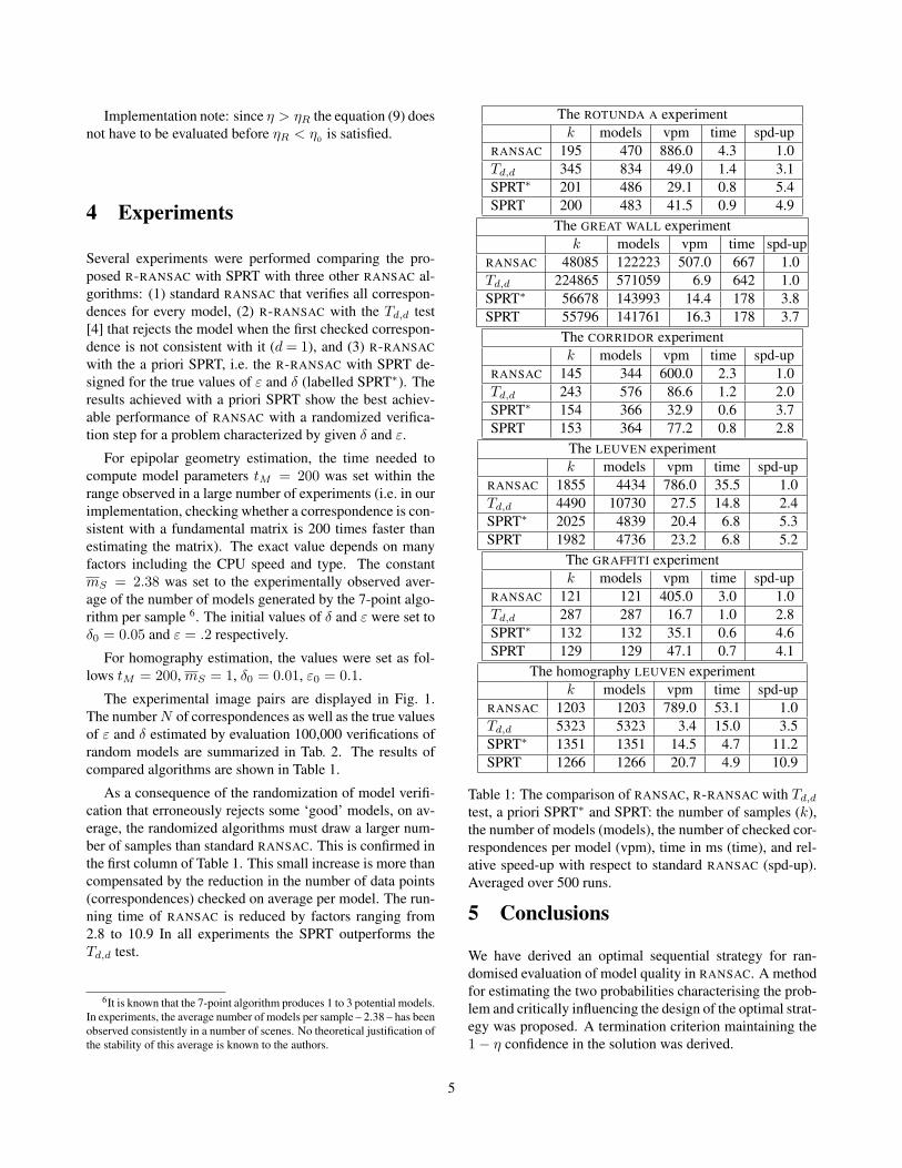
The experimental image pairs are displayed in Fig. 1.The number N of correspondences as well as the true valuesof ε and δ estimated by evaluation 100,000 verifications ofrandom models are summarized in Tab. 2. The results ofcompared algorithms are shown in Table 1.

As a consequence of the randomization of model verifi-cation that erroneously rejects some ‘good’ models, on av-erage, the randomized algorithms must draw a larger num-ber of samples than standard RANSAC. This is confirmed inthe first column of Table 1. This small increase is more thancompensated by the reduction in the number of data points(correspondences) checked on average per model. The run-ning time of RANSAC is reduced by factors ranging from2.8 to 10.9 In all experiments the SPRT outperforms theTd,d test.

6It is known that the 7-point algorithm produces 1 to 3 potential models.In experiments, the average number of models per sample – 2.38 – has beenobserved consistently in a number of scenes. No theoretical justification ofthe stability of this average is known to the authors.

The ROTUNDA A experimentk models vpm time spd-up

RANSAC 195 470 886.0 4.3 1.0Td,d 345 834 49.0 1.4 3.1SPRT∗ 201 486 29.1 0.8 5.4SPRT 200 483 41.5 0.9 4.9

The GREAT WALL experimentk models vpm time spd-up

RANSAC 48085 122223 507.0 667 1.0Td,d 224865 571059 6.9 642 1.0SPRT∗ 56678 143993 14.4 178 3.8SPRT 55796 141761 16.3 178 3.7

The CORRIDOR experimentk models vpm time spd-up

RANSAC 145 344 600.0 2.3 1.0Td,d 243 576 86.6 1.2 2.0SPRT∗ 154 366 32.9 0.6 3.7SPRT 153 364 77.2 0.8 2.8

The LEUVEN experimentk models vpm time spd-up

RANSAC 1855 4434 786.0 35.5 1.0Td,d 4490 10730 27.5 14.8 2.4SPRT∗ 2025 4839 20.4 6.8 5.3SPRT 1982 4736 23.2 6.8 5.2

The GRAFFITI experimentk models vpm time spd-up

RANSAC 121 121 405.0 3.0 1.0Td,d 287 287 16.7 1.0 2.8SPRT∗ 132 132 35.1 0.6 4.6SPRT 129 129 47.1 0.7 4.1

The homography LEUVEN experimentk models vpm time spd-up

RANSAC 1203 1203 789.0 53.1 1.0Td,d 5323 5323 3.4 15.0 3.5SPRT∗ 1351 1351 14.5 4.7 11.2SPRT 1266 1266 20.7 4.9 10.9

Table 1: The comparison of RANSAC, R-RANSAC with Td,d

test, a priori SPRT∗ and SPRT: the number of samples (k),the number of models (models), the number of checked cor-respondences per model (vpm), time in ms (time), and rel-ative speed-up with respect to standard RANSAC (spd-up).Averaged over 500 runs.

5 Conclusions

We have derived an optimal sequential strategy for ran-domised evaluation of model quality in RANSAC. A methodfor estimating the two probabilities characterising the prob-lem and critically influencing the design of the optimal strat-egy was proposed. A termination criterion maintaining the1− η confidence in the solution was derived.

5

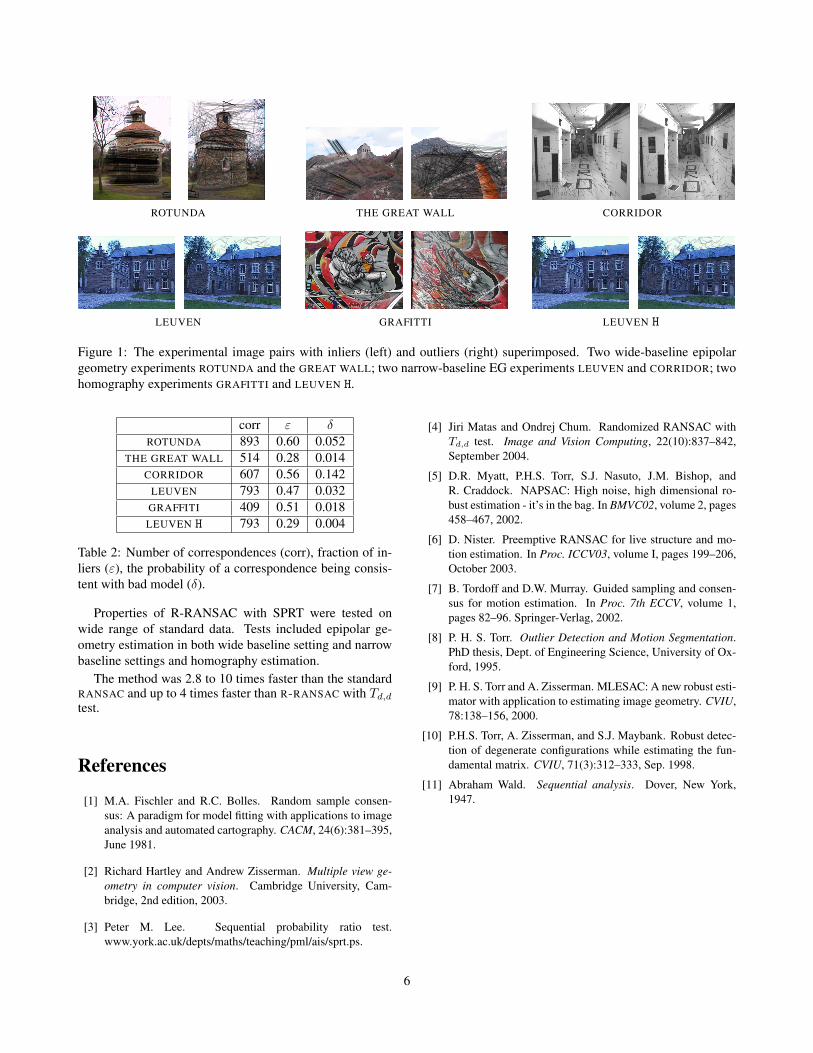
ROTUNDA THE GREAT WALL CORRIDOR

LEUVEN GRAFITTI LEUVEN H

Figure 1: The experimental image pairs with inliers (left) and outliers (right) superimposed. Two wide-baseline epipolargeometry experiments ROTUNDA and the GREAT WALL; two narrow-baseline EG experiments LEUVEN and CORRIDOR; twohomography experiments GRAFITTI and LEUVEN H.

corr ε δROTUNDA 893 0.60 0.052

THE GREAT WALL 514 0.28 0.014CORRIDOR 607 0.56 0.142

LEUVEN 793 0.47 0.032GRAFFITI 409 0.51 0.018LEUVEN H 793 0.29 0.004

Table 2: Number of correspondences (corr), fraction of in-liers (ε), the probability of a correspondence being consis-tent with bad model (δ).

Properties of R-RANSAC with SPRT were tested onwide range of standard data. Tests included epipolar ge-ometry estimation in both wide baseline setting and narrowbaseline settings and homography estimation.

The method was 2.8 to 10 times faster than the standardRANSAC and up to 4 times faster than R-RANSAC with Td,d

test.

References

[1] M.A. Fischler and R.C. Bolles. Random sample consen-sus: A paradigm for model fitting with applications to imageanalysis and automated cartography. CACM, 24(6):381–395,June 1981.

[2] Richard Hartley and Andrew Zisserman. Multiple view ge-ometry in computer vision. Cambridge University, Cam-bridge, 2nd edition, 2003.

[3] Peter M. Lee. Sequential probability ratio test.www.york.ac.uk/depts/maths/teaching/pml/ais/sprt.ps.

[4] Jiri Matas and Ondrej Chum. Randomized RANSAC withTd,d test. Image and Vision Computing, 22(10):837–842,September 2004.

[5] D.R. Myatt, P.H.S. Torr, S.J. Nasuto, J.M. Bishop, andR. Craddock. NAPSAC: High noise, high dimensional ro-bust estimation - it’s in the bag. In BMVC02, volume 2, pages458–467, 2002.

[6] D. Nister. Preemptive RANSAC for live structure and mo-tion estimation. In Proc. ICCV03, volume I, pages 199–206,October 2003.

[7] B. Tordoff and D.W. Murray. Guided sampling and consen-sus for motion estimation. In Proc. 7th ECCV, volume 1,pages 82–96. Springer-Verlag, 2002.

[8] P. H. S. Torr. Outlier Detection and Motion Segmentation.PhD thesis, Dept. of Engineering Science, University of Ox-ford, 1995.

[9] P. H. S. Torr and A. Zisserman. MLESAC: A new robust esti-mator with application to estimating image geometry. CVIU,78:138–156, 2000.

[10] P.H.S. Torr, A. Zisserman, and S.J. Maybank. Robust detec-tion of degenerate configurations while estimating the fun-damental matrix. CVIU, 71(3):312–333, Sep. 1998.

[11] Abraham Wald. Sequential analysis. Dover, New York,1947.

6