
Randomized Matrix Dompositions Using R - arXiv
47
Randomized Matrix Decompositions Using R N. Benjamin Erichson University of St Andrews Sergey Voronin Tufts University Steven L. Brunton University of Washington J. Nathan Kutz University of Washington Abstract Matrix decompositions are fundamental tools in the area of applied mathematics, statistical computing, and machine learning. In particular, low-rank matrix decompo- sitions are vital, and widely used for data analysis, dimensionality reduction, and data compression. Massive datasets, however, pose a computational challenge for traditional algorithms, placing significant constraints on both memory and processing power. Re- cently, the powerful concept of randomness has been introduced as a strategy to ease the computational load. The essential idea of probabilistic algorithms is to employ some amount of randomness in order to derive a smaller matrix from a high-dimensional data matrix. The smaller matrix is then used to compute the desired low-rank approximation. Such algorithms are shown to be computationally efficient for approximating matrices with low-rank structure. We present the R package rsvd, and provide a tutorial introduction to randomized matrix decompositions. Specifically, randomized routines for the singular value decomposition, (robust) principal component analysis, interpolative decomposition, and CUR decomposition are discussed. Several examples demonstrate the routines, and show the computational advantage over other methods implemented in R. Keywords : dimension reduction, randomized algorithm, low-rank approximations, singular value decomposition, principal component analysis, CUR decomposition, R. 1. Introduction In the era of “big data”, vast amounts of data are being collected and curated in the form of arrays across the social, physical, engineering, biological, and ecological sciences. Analysis of the data relies on a variety of matrix decomposition methods which seek to exploit low-rank features exhibited by the high-dimensional data. Indeed, matrix decompositions are often the workhorse algorithms for scientific computing applications in the areas of applied mathematics, statistical computing, and machine learning. Despite our ever-increasing computational power, the emergence of large-scale datasets has severely challenged our ability to analyze data using traditional matrix algorithms. Moreover, the growth of data collection is far outstripping computational performance gains. The computationally expensive singular value decomposition (SVD) is the most ubiquitous method for dimensionality reduction, data processing and compression. The concept of randomness has recently been demonstrated as an effective strategy to easing the computational demands of low-rank approximations from arXiv:1608.02148v5 [stat.CO] 26 Nov 2019
Transcript of Randomized Matrix Dompositions Using R - arXiv

Randomized Matrix Decompositions Using R
N. Benjamin ErichsonUniversity of St Andrews
Sergey VoroninTufts University
Steven L. BruntonUniversity of Washington
J. Nathan KutzUniversity of Washington
Abstract
Matrix decompositions are fundamental tools in the area of applied mathematics,statistical computing, and machine learning. In particular, low-rank matrix decompo-sitions are vital, and widely used for data analysis, dimensionality reduction, and datacompression. Massive datasets, however, pose a computational challenge for traditionalalgorithms, placing significant constraints on both memory and processing power. Re-cently, the powerful concept of randomness has been introduced as a strategy to easethe computational load. The essential idea of probabilistic algorithms is to employ someamount of randomness in order to derive a smaller matrix from a high-dimensional datamatrix. The smaller matrix is then used to compute the desired low-rank approximation.Such algorithms are shown to be computationally efficient for approximating matrices withlow-rank structure. We present the R package rsvd, and provide a tutorial introductionto randomized matrix decompositions. Specifically, randomized routines for the singularvalue decomposition, (robust) principal component analysis, interpolative decomposition,and CUR decomposition are discussed. Several examples demonstrate the routines, andshow the computational advantage over other methods implemented in R.
Keywords: dimension reduction, randomized algorithm, low-rank approximations, singularvalue decomposition, principal component analysis, CUR decomposition, R.
1. Introduction
In the era of “big data”, vast amounts of data are being collected and curated in the form ofarrays across the social, physical, engineering, biological, and ecological sciences. Analysis ofthe data relies on a variety of matrix decomposition methods which seek to exploit low-rankfeatures exhibited by the high-dimensional data. Indeed, matrix decompositions are often theworkhorse algorithms for scientific computing applications in the areas of applied mathematics,statistical computing, and machine learning. Despite our ever-increasing computationalpower, the emergence of large-scale datasets has severely challenged our ability to analyzedata using traditional matrix algorithms. Moreover, the growth of data collection is faroutstripping computational performance gains. The computationally expensive singular valuedecomposition (SVD) is the most ubiquitous method for dimensionality reduction, dataprocessing and compression. The concept of randomness has recently been demonstrated asan effective strategy to easing the computational demands of low-rank approximations from
arX
iv:1
608.
0214
8v5
[st
at.C
O]
26
Nov
201
9

2 Randomized Matrix Decompositions Using R
matrix decompositions such as the SVD, thus allowing for a scalable architecture for modern“big data” applications. Throughout this paper, we make the following assumption: the datamatrix to be approximated has low-rank structure, i.e., the rank is smaller than the ambientdimension of the measurement space.
1.1. Randomness as a computational strategy
Randomness is a fascinating and powerful concept in science and nature. Probabilisticconcepts can be used as an effective strategy for designing better algorithms. By the deliberateintroduction of randomness into computations (Motwani and Raghavan 1995), randomizedalgorithms have not only been shown to outperform some of the best deterministic methods,but they have also enabled the computation of previously infeasible problems. The MonteCarlo method, invented by Stan Ulam, Nick Metropolis and John von Neumann, is among themost prominent randomized methods in computational statistics as well as one of the “best”algorithms of the 20th century (Cipra 2000).Over the past two decades, probabilistic algorithms have been established to compute matrixapproximations, forming the field of randomized numerical linear algebra (Drineas and Mahoney2016). While randomness is quite controversial, and is often seen as an obstacle and a nuisance,modern randomized matrix algorithms are reliable and numerically stable. The basic ideaof probabilistic matrix algorithms is to employ a degree of randomness in order to derivea smaller matrix from a high-dimensional matrix, which captures the essential information.Thus, none of the “randomness” should obscure the dominant spectral information of the dataas long as the input matrix features some low-rank structure. Then, a deterministic matrixfactorization algorithm is applied to the smaller matrix to compute a near-optimal low-rankapproximation. The principal concept is sketched in Figure 1.Several probabilistic strategies have been proposed to find a “good” smaller matrix, and werefer the reader to the surveys by Mahoney (2011), Liberty (2013), and Halko, Martinsson,and Tropp (2011b) for an in-depth discussion, and theoretical results. In addition to computingthe singular value decomposition (Sarlos 2006; Martinsson, Rokhlin, and Tygert 2011) andprincipal component analysis (Rokhlin, Szlam, and Tygert 2009; Halko, Martinsson, Shkolnisky,and Tygert 2011a), it has been demonstrated that this probabilistic framework can also be
A factors
B approximatedfactors
deterministic algorithm
deterministic algorithm
probabilistic strategyto find a small matrix
recover near-optimal factors
Data Decomposition
“Big”
“Small”
Figure 1: First, randomness is used as a computational strategy to derive a smaller matrixB from A. Then, the low-dimensional matrix is used to compute an approximate matrixdecomposition. Finally, the near-optimal (high-dimensional) factors may be reconstructed.

N. Benjamin Erichson, Sergey Voronin, Steven L. Brunton, J. Nathan Kutz 3
used to compute the pivoted QR decomposition (Duersch and Gu 2017), the pivoted LUdecomposition (Shabat, Shmueli, Aizenbud, and Averbuch 2016), and the dynamic modedecomposition (Erichson, Brunton, and Kutz 2017).
1.2. The rsvd package: Motivation and contributions
The computational costs of applying deterministic matrix algorithms to massive data matricescan render the problem intractable. Randomized matrix algorithms are becoming increasinglypopular as an alternative, and implementations are available in a variety of programminglanguages and machine learning libraries. For instance, Voronin and Martinsson (2015) providehigh performance, multi-core and GPU accelerated randomized routines in C.The rsvd package aims to fill the gap in R, providing the following randomized routines:
• Randomized singular value decomposition: rsvd().• Randomized principal component analysis: rpca().• Randomized robust principal component analysis: rrpca().• Randomized interpolative decomposition: rid().• Randomized CUR decomposition: rcur().
The routines are, in particular, efficient for matrices with rapidly decaying singular values.Figure 2 compares the computational performance of the rsvd() function to other existingSVD routines in R, which are discussed in more detail in Section 3.5. Specifically, for computingthe dominant k singular values and vectors, the randomized singular value decompositionfunction rsvd() results in significant speedups over other existing SVD routines in R. SeeSection 3.8 for a more detailed performance evaluation.The computational benefits of the randomized SVD translates directly to principal componentanalysis (PCA), since both methods are closely related. Further, the randomized SVD can beused to accelerate the computation of robust principal component analysis (RPCA). Moregenerally, the concept of randomness allows also one to efficiently compute modern matrix
3000 x 2000 5000 x 3000 10000 x 5000
svd
propack
RSpectra
irlba
rsvd
svd
propack
RSpectra
irlba
rsvd
svd
propack
RSpectra
irlba
rsvd
0
20
40
60
80
100
120
Speedup o
ver
base s
vd
Figure 2: Runtime speedups (relative performance) of fast SVD algorithms compared to thebase svd() routine in R. Here, the dominant k = 20 singular values and vectors are computedfor random low-rank matrices with varying dimension m×n. Note, here we are using MicrosoftOpen 3.5.1 which provides the Intel MKL for parallel mathematical computing (using 4 cores).

4 Randomized Matrix Decompositions Using R
decompositions such as the interpolative decomposition (ID) and CUR decomposition. Whilethe performance of the randomized algorithms depends on the actual shape of the matrix,we can state (as a rule of thumb) that significant computational speedups are achieved if thetarget rank k is about 3-6 times smaller than the smallest dimension minm,n of the matrix.The speedup for tall and thin matrices is in general less impressive than for “big” fat matrices.The rsvd package is available from the Comprehensive R Archive Network (CRAN) at https://CRAN.R-project.org/package=rsvd. Thus, to install and load within R simply use:
R> install.packages("rsvd")R> library("rsvd")
Alternatively, the package can be obtained via github: https://github.com/erichson/rSVD.
1.3. Organization
The remainder of this paper is organized as follows. First, Section 2 outlines the advocatedprobabilistic framework for low-rank matrix approximations. Section 3 briefly reviews thesingular value decomposition and the randomized SVD algorithm. Then, the rsvd() functionand its computational performance are demonstrated. Section 4 first describes the principalcomponent analysis. Then, the randomized PCA algorithm is outlined, followed by thedemonstration of the corresponding rpca() function. Section 5 outlines robust principalcomponent analysis, and describes the randomized robust PCA algorithm as well as the rrpca()function. Section 6 gives a high-level overview of the interpolative and CUR decomposition.Finally, concluding remarks and a roadmap for future developments are presented in Section 7.
1.4. Notation
In the following we give a brief overview of some notation used throughout this manuscript.Scalars are denoted by lower case letters x, and vectors both in Rn and Cn are denoted asbold lower case letters x = [x1, x2, . . . , xn]>. Matrices are denoted by bold capital letters Aand the entry at row i and column j is denoted as A(i, j). This notation is convenient formatrix slicing, for instance, A(1 : i, :) extracts the first 1, 2, . . . , i rows, and A(:, 1 : j) extractsthe first 1, 2, . . . , j columns. The transpose of a real matrix is denoted as A>, and withoutloss of generality, we restrict most of the discussion in the following to real matrices. Further,the column space (range) of A is denoted as col(A), and the row space as row(A).The spectral or operator norm of a matrix is defined as the largest singular value σmax of A,i.e., the square root of the largest eigenvalue λmax of the positive-semidefinite matrix A>A:
‖A‖2 =√λmax(A>A) = σmax(A) = max
x6=0
‖Ax‖2‖x‖2
.
The Frobenius norm is defined as the square root of the sum of the absolute squares of itselements, which is equal to the square root of the matrix trace of A>A:
‖A‖F =
√√√√ m∑i=1
n∑j=1|A(i, j)|2 =
√trace(A>A).

N. Benjamin Erichson, Sergey Voronin, Steven L. Brunton, J. Nathan Kutz 5
2. Probabilistic framework for low-rank approximationsAssume that a matrix A ∈ Rm×n has rank r, where r ≤ minm,n. Then, in general, theobjective of a low-rank matrix approximation is to find two smaller matrices such that:
A ≈ E F,m× n m× r r × n (1)
where the columns of the matrix E ∈ Rm×r span the column space of A, and the rows ofthe matrix F ∈ Rr×n span the row space of A. The factors E and F can then be used tosummarize or to reveal some interesting structure in the data. Further, the factors can beused to efficiently store the large data matrix A. Specifically, while A requires mn words ofstorage, E and F require only mr + nr words of storage.In practice, most data matrices do not feature a precise rank r. Rather we are commonlyinterested in finding a rank-k matrix Ak, which is as close as possible to an arbitrary inputmatrix A in the least-square sense. We refer to k as the target rank in the following.In particular, modern data analysis and scientific computing largely rely on low-rank approxi-mations, since low-rank matrices are ubiquitous throughout the sciences. However, in the eraof “big data”, the emergence of massive data poses a significant computational challenge fortraditional deterministic algorithms.In the following, we advocate the probabilistic framework, formulated by Halko et al. (2011b),to compute a near-optimal low-rank approximation. Conceptually, this framework splits thecomputational task into two logical stages:
• Stage A: Construct a low dimensional subspace that approximates the column space ofA. This means, the aim is to find a matrix Q ∈ Rm×k with orthonormal columns suchthat A ≈ QQ>A is satisfied.
• Stage B: Form a smaller matrix B := Q>A ∈ Rk×n, i.e., restrict the high-dimensionalinput matrix to the low-dimensional space spanned by the near-optimal basis Q. Thesmaller matrix B can then be used to compute a desired low-rank approximation.
The first computational stage is where randomness comes into the play, while the second stageis purely deterministic. In the following, the two stages are described in detail.
2.1. The generic randomized algorithm
Stage A: Computing the near-optimal basis
First, we aim to find a near-optimal basis Q for the matrix A such that
A ≈ QQ>A (2)
is satisfied. The desired target rank k is assumed to be k minm,n. Specifically, P := QQ>is a linear orthogonal projector. A projection operator corresponds to a linear subspace, andtransforms any vector to its orthogonal projection on the subspace. This is illustrated inFigure 3, where a vector x is confined to the column space col(A).

6 Randomized Matrix Decompositions Using R
origin
x = Px
x
col(A)
Figure 3: Geometric illustration of the orthogonal projection operator P. A vector x ∈ Rm isrestricted to the column space of A, where Px ∈ col(A).
The concept of random projections can be used to sample the range (column space) of the inputmatrix A in order to efficiently construct such a orthogonal projector. Random projectionsare data agnostic, and constructed by first drawing a set of k random vectors ωiki=1, forinstance, from the standard normal distribution. Probability theory guarantees that randomvectors are linearly independent with high probability. Then, a set of random projectionsyiki=1 is computed by mapping A to low-dimensional space:
yi := Aωi for i = 1, 2, . . . , k. (3)
In other words, this process forms a set of independent randomly weighted linear combinationsof the columns of A, and reduces the number of columns from n to k. While the input matrixis compressed, the Euclidean distances between the original data points are approximatelypreserved. Random projections are also well known as the Johnson-Lindenstrauss (JL)transform (Johnson and Lindenstrauss 1984), and we refer to Ahfock, Astle, and Richardson(2017) for a recent statistical perspective.Equation 3 can be efficiently executed in parallel. Therefore, let us define the random testmatrix Ω ∈ Rn×k, which is again drawn from the standard normal distribution, and thecolumns of which are given by the vectors ωi. The samples matrix Y ∈ Rm×k, also denotedas sketch, is then obtained by post-multiplying the input matrix by the random test matrix
Y := AΩ. (4)
Once Y is obtained, it only remains to orthonormalize the columns in order to form a naturalbasis Q ∈ Rm×k. This can be efficiently achieved using the QR-decomposition Y =: QR, andit follows that Equation 2 is satisfied.
Stage B: Compute the smaller matrix
Now, given the near-optimal basis Q, we aim to find a smaller matrix B ∈ Rk×n. Therefore,we project the high-dimensional input matrix A to low-dimensional space
B := Q>A. (5)
Geometrically, this is a projection (i.e., a linear transformation) which takes points in ahigh-dimensional space into corresponding points in a low-dimensional space, illustrated in

N. Benjamin Erichson, Sergey Voronin, Steven L. Brunton, J. Nathan Kutz 7
Rm
projection
Rk
Figure 4: Points in a high-dimensional space are projected into low-dimensional space, whilethe geometric structure is preserved in an Euclidean sense.
Figure 4. This process preserves the geometric structure of the data in an Euclidean sense,i.e., the length of the projected vectors as well as the angles between the projected vectorsare preserved. This is, due to the invariance of inner products (Trefethen and Bau 1997).Substituting Equation 5 into 2 yields then the following low-rank approximation
A ≈ Q B.m× n m× k k × n
This decomposition is referred to as the QB decomposition. Subsequently, the smaller matrixB can be used to compute a matrix decomposition using a traditional algorithm.
2.2. Improved randomized algorithm
The basis matrix Q often fails to provide a good approximation for the column space of theinput matrix. This is because most real-world data matrices do not feature a precise rank r,and instead exhibit a gradually decaying singular value spectrum. The performance can beconsiderably improved using the concept of oversampling and the power iteration scheme.
Oversampling
Most data matrices do not feature an exact rank, which means that the singular valuesσini=k+1 of the input matrix A are non-zero. As a consequence, the sketch Y does notexactly span the column space of the input matrix. Oversampling can be used to overcomethis issue by using l := k+ p random projections to form the sketch, instead of just k. Here, pdenotes the number of additional projections, and a small number p = 5, 10 is often sufficientto obtain a good basis that is comparable to the best possible basis (Martinsson 2016).The intuition behind the oversampling scheme is the following. The sketch Y is a randomvariable, as it depends on the drawing of a random test matrix Ω. Increasing the numberof additional random projections allows one to decrease the variation in the singular valuespectrum of the random test matrix, which subsequently improves the quality of the sketch.
Power iteration scheme
The second method for improving the quality of the basis Q involves the concept of powersampling iterations (Rokhlin et al. 2009; Halko et al. 2011b; Gu 2015). Instead of obtainingthe sketch Y directly, the data matrix A is first preprocessed as
A(q) := (AA>)qA, (6)

8 Randomized Matrix Decompositions Using R
0 10 20 30 40 50Singular values, i
0.0
0.5
1.0
Mag
nitu
de
true singular valuesq=1q=2q=3
Figure 5: Singular value spectrum of a low-rank (r = 30) matrix before and after preprocessing.The computation of power iterations enforce a more rapid decay of singular values.
where q is an integer specifying the number of power iterations. This process enforces a morerapid decay of the singular values. Thus, we enable the algorithm to sample the relevantinformation related to the dominant singular values, while unwanted information is suppressed.Let A = UΣV> be the singular value decomposition. It is simple to show that A(q) :=(AA>)qA = UΣ2q+1V>. Here, U and V are orthonormal matrices whose columns are theleft and right singular vectors of A, and Σ is a diagonal matrix containing the singular valuesin descending order. Hence, for q > 0, the modified matrix A(q) has a relatively fast decay ofsingular values even when the decay in A is modest. This is illustrated in Figure 5, showingthe singular values of a 50× 50 low-rank matrix before (red) and after computing q = 1, 2, 3power iterations. Thus, substituting Equation 6 into 4 yields an improved sketch
Y := A(q)Ω.
When the singular values of the data matrix decay slowly, as few as q = 1, 2, 3 poweriterations can considerably improve the accuracy of the approximation. The drawback of thepower scheme is that q additional passes over the input matrix are required.Algorithm 1 shows a direct implementation of the power iteration scheme. Due to potentialround-off errors, however, this algorithm is not recommended in practice.The numerical stability can be improved by orthogonalizing the sketch between each iteration.This scheme is shown in Algorithm 2, and denoted as subspace iteration (Halko et al. 2011b;Gu 2015). The pivoted LU decomposition can be used as an intermediate step instead of theQR decomposition as proposed by Rokhlin et al. (2009). Algorithm 3 is computationally moreefficient, while slightly less accurate.
2.3. Random test matrices
The probabilistic framework above essentially depends on the random test matrix Ω usedfor constructing the sketch Y. Specifically, we seek a matrix with independent identicallydistributed (i.i.d.) entries from some distribution, which ensures that its columns are linearlyindependent with high probability. Some popular choices for constructing the random testmatrix are:

N. Benjamin Erichson, Sergey Voronin, Steven L. Brunton, J. Nathan Kutz 9
Input: Input matrix A, the sketch Y, and parameter q.function power_iterations(A,Y, q)(1) for j = 1, . . . , q perform q power iterations(2) Y = A>Y(3) Y = AYReturn: Y ∈ Rm×k
Algorithm 1: Direct implementation of the power scheme.
Input: Input matrix A, the sketch Y, and q.function sub_iterations(A,Y, q)(1) for j = 1, . . . , q perform q iterations(2) [Q,∼] = qr(Y) economic QR(3) [Q,∼] = qr(A>Q) economic QR(4) Y = AQReturn: Y ∈ Rm×k
Algorithm 2: Subspace iterations.
Input: Input matrix A, the sketch Y, and q.function norm_iterations(A,Y, q)(1) for j = 1, . . . , q perform q iterations(2) [L,∼] = lu(Y) pivoted LU(3) [L,∼] = lu(A>L) pivoted LU(4) Y = ALReturn: Y ∈ Rm×k
Algorithm 3: Normalized power iterations.
• Gaussian. The default choice to construct a random test matrix is to draw entries fromthe standard normal distribution, N (0, 1). The normal distribution is known to haveexcellent performance for sketching in practice. Further, the theoretical properties of thenormal distribution enable the derivation of accurate error bounds (Halko et al. 2011b).
• Uniform. A simple alternative is to draw entries from the uniform distribution, U(−1, 1).While the behavior is similar in practice, the generation of uniform random samples iscomputationally more efficient.
• Rademacher. Yet another approach to construct the random test matrix is to drawindependent Rademacher entries. The Rademacher distribution is a discrete probabilitydistribution, where the random variates take the values +1 and −1 with equal probability.Rademacher entries are simple to generate, and they are cheaper to store than Gaussianand uniform random test matrices (Tropp, Yurtsever, Udell, and Cevher 2016).
Currently, the rsvd package only supports standard dense random test matrices; however,dense matrix operations can become very expensive for large-scale applications. This is

10 Randomized Matrix Decompositions Using R
because it takes O(mnk) time to apply an n × k dense random test matrix to any m × ndense input matrix. Structured random test matrices provide a computationally more efficientalternative (Woolfe, Liberty, Rokhlin, and Tygert 2008), reducing the costs to O(mn log(k)).Very sparse random test matrices are even simpler to construct (Li, Hastie, and Church 2006),yet slightly less accurate. These can be applied to any m× n dense matrix in O(m nnz(Ω))using sparse matrix multiplication routines, where nnz() denotes the non-zero entries in thesparse random test matrix.
3. Randomized singular value decompositions
The SVD provides a numerically stable matrix decomposition that can be used to obtainlow-rank approximations, to compute the pseudo-inverses of non-square matrices, and to findthe least-squares and minimum norm solutions of a linear model. Further, the SVD is theworkhorse algorithm behind many machine learning concepts, for instance, matrix completion,sparse coding, dictionary learning, PCA and robust PCA. For a comprehensive technicaloverview of the SVD we refer to Golub and Van Loan (1996), and Trefethen and Bau (1997).
3.1. Brief historical overview
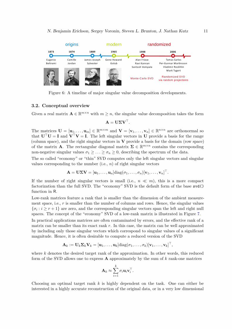
While the origins of the SVD can be traced back to the late 19th century, the field ofrandomized matrix algorithms is relatively young. Figure 6 shows a short time-line of somemajor developments of the singular value decomposition. Stewart (1993) gives an excellenthistorical review of the five mathematicians who developed the fundamentals of the SVD,namely Eugenio Beltrami (1835–1899), Camille Jordan (1838–1921), James Joseph Sylvester(1814–1897), Erhard Schmidt (1876–1959) and Hermann Weyl (1885–1955). The developmentand fundamentals of modern high-performance algorithms to compute the SVD are relatedto the seminal work of Golub and Kahan (1965) and Golub and Reinsch (1970), forming thebasis for the EISPACK, and LAPACK SVD routines.
Modern partial singular value decomposition algorithms are largely based on Krylov methods,such as the Lanczos algorithm (Calvetti, Reichel, and Sorensen 1994; Larsen 1998; Lehoucq,Sorensen, and Yang 1998; Baglama and Reichel 2005). These methods are accurate and areparticularly powerful for approximating structured, and sparse matrices.
Randomized matrix algorithms for computing low-rank matrix approximations have gainedprominence over the past two decades. Frieze, Kannan, and Vempala (2004) introduced the“Monte Carlo” SVD, a rigorous approach to efficiently compute the approximate low-rank SVDbased on non-uniform row and column sampling. Sarlos (2006), Liberty, Woolfe, Martinsson,Rokhlin, and Tygert (2007) and Martinsson et al. (2011) introduced a more robust approachbased on random projections. Specifically, the properties of random vectors are exploitedto efficiently build a subspace that captures the column space of a matrix. Woolfe et al.(2008) further improved the computational performance by leveraging the properties of highlystructured matrices, which enable fast matrix multiplications. Eventually, the seminal workby Halko et al. (2011b) unified and expanded previous work on the randomized singularvalue decomposition and introduced state-of-the-art prototype algorithms to compute thenear-optimal low-rank singular value decomposition.
N. Benjamin Erichson, Sergey Voronin, Steven L. Brunton, J. Nathan Kutz 11
Figure 6: A timeline of major singular value decomposition developments.
3.2. Conceptual overview
Given a real matrix A ∈ Rm×n with m ≥ n, the singular value decomposition takes the form
A = UΣV>.
The matrices U = [u1, . . . ,um] ∈ Rm×m and V = [v1, . . . ,vn] ∈ Rn×n are orthonormal sothat U>U = I and V>V = I. The left singular vectors in U provide a basis for the range(column space), and the right singular vectors in V provide a basis for the domain (row space)of the matrix A. The rectangular diagonal matrix Σ ∈ Rm×n contains the correspondingnon-negative singular values σ1 ≥ . . . ≥ σn ≥ 0, describing the spectrum of the data.The so called “economy” or “thin” SVD computes only the left singular vectors and singularvalues corresponding to the number (i.e., n) of right singular vectors
A = UΣV = [u1, . . . ,un]diag(σ1, . . . , σn)[v1, . . . ,vn]>.
If the number of right singular vectors is small (i.e., n m), this is a more compactfactorization than the full SVD. The “economy” SVD is the default form of the base svd()function in R.Low-rank matrices feature a rank that is smaller than the dimension of the ambient measure-ment space, i.e., r is smaller than the number of columns and rows. Hence, the singular valuesσi : i ≥ r + 1 are zero, and the corresponding singular vectors span the left and right nullspaces. The concept of the “economy” SVD of a low-rank matrix is illustrated in Figure 7.In practical applications matrices are often contaminated by errors, and the effective rank of amatrix can be smaller than its exact rank r. In this case, the matrix can be well approximatedby including only those singular vectors which correspond to singular values of a significantmagnitude. Hence, it is often desirable to compute a reduced version of the SVD
Ak := UkΣkVk = [u1, . . . ,uk]diag(σ1, . . . , σk)[v1, . . . ,vk]>,
where k denotes the desired target rank of the approximation. In other words, this reducedform of the SVD allows one to express A approximately by the sum of k rank-one matrices
Ak ≈k∑
i=1σiuiv>i .
Choosing an optimal target rank k is highly dependent on the task. One can either beinterested in a highly accurate reconstruction of the original data, or in a very low dimensional

12 Randomized Matrix Decompositions Using R
=
Figure 7: Schematic of the “economy” SVD for a rank-r matrix, where m ≥ n.
representation of dominant features in the data. In the former case k should be chosen closeto the effective rank, while in the latter case k might be chosen to be much smaller.Truncating small singular values in the deterministic SVD gives an optimal approximation ofthe corresponding target rank k. Specifically, the Eckart-Young theorem (Eckart and Young1936) states that the low-rank SVD provides the optimal rank-k reconstruction of a matrix inthe least-square sense
Ak := argminrank(A′
k)=k‖A−A′k‖.
The reconstruction error in both the spectral and Frobenius norms is given by
‖A−Ak‖2 = σk+1(A) and ‖A−Ak‖F =
√√√√√min(m,n)∑j=k+1
σ2j (A).
For massive datasets, however, the truncated SVD is costly to compute. The cost to computethe full SVD of an m× n matrix is of the order O(mn2), from which the first k componentscan then be extracted to form Ak.
3.3. Randomized algorithm
Randomized algorithms have been recently popularized, in large part due to their “surprising”reliability and computational efficiency (Gu 2015). These techniques can be used to obtain anapproximate rank-k singular value decomposition at a cost of O(mnk). When the dimensionsof A are large, this is substantially more efficient than truncating the full SVD.We present details of the randomized low-rank SVD algorithm, which comes with favorableerror bounds relative to the optimal truncated SVD, as presented in the seminal paper by Halkoet al. (2011b), and further analyzed and implemented in Voronin and Martinsson (2015).Let A ∈ Rm×n be a low-rank matrix, and without loss of generality m ≥ n. In the following,we seek the near-optimal low-rank approximation of the form
A ≈ UkΣkV>k ,

N. Benjamin Erichson, Sergey Voronin, Steven L. Brunton, J. Nathan Kutz 13
'economic'
QR=
=
=
SVD
recover lesingular vectors
Figure 8: Conceptual architecture of the randomized singular value decomposition (rSVD).First, a natural basis Q is computed in order to derive the smaller matrix B. Then, the SVDis efficiently computed using this smaller matrix. Finally, the left singular vectors U may bereconstructed from the approximate singular vectors U by the expression in Equation 7.
where k denotes the target rank. Instead of computing the singular value decompositiondirectly, we embed the SVD into the probabilistic framework presented in Section 2. Theprincipal concept is sketched in Figure 8.Specifically, we first compute the near-optimal basis Q ∈ Rm×l using the randomized scheme asoutlined in detail above. Note that we allow for both oversampling (l = k+ p), and additionalpower iterations q, in order to obtain the near-optimal basis matrix. The matrix B ∈ Rl×n isrelatively small if l n, and it is obtained by projecting the input matrix to low-dimensionalspace, i.e., B := Q>A. The full SVD of B is then computed using a deterministic algorithm
B = UΣV>.
Thus, we efficiently obtain the first l right singular vectors V ∈ Rn×l as well as the correspondingsingular values Σ ∈ Rl×l. It remains to recover the left singular vectors U ∈ Rm×l from theapproximate left singular vectors U ∈ Rl×l by pre-multiplying by Q
U ≈ QU. (7)

14 Randomized Matrix Decompositions Using R
Input: Input matrix A with dimensions m× n, and target rank k < minm,n.Optional: Parameters p and q to control oversampling, and the power scheme.
function rqb(A, k, p, q)
(1) l = k + p slight oversampling(2) Ω = rnorm(n, l) generate random test matrix(3) Y = AΩ compute sketch(4) Y = sub_iterations(A,Y, q) optional: compute power scheme via Algorithm 2(9) [Q,∼] = qr(Y) form orthonormal basis(10) B = Q>A project to low-dimensional space
Return: Q ∈ Rm×l, B ∈ Rl×n
Algorithm 4: A randomized QB decomposition algorithm.
The justification for the randomized SVD can be sketched as follows
A ≈ QQ>A = QB = QUΣV> = UΣV>.
Algorithm 5 presents an implementation using the randomized QB decomposition in Al-gorithm 4. The approximation quality can be controlled via oversampling and additionalsubspace iterations. Note that if an oversampling parameter p > 0 has been specified, thedesired rank-k approximation is simply obtained by truncating the left and right singularvectors and the singular values.The randomized singular value decomposition has several practical advantages:
• Lower communication costs. The randomized algorithm presented here requiresfew (at least two) passes over the input matrix. By passes we refer to the number ofsequential reads of the entire input matrix. This aspect is crucial in the area of “big data”where communication costs play a significant role. For instance, the time to transfer thedata from the hard-drive into fast memory can be substantially more expensive thanthe theoretical costs of the algorithm would suggest. Recently, Tropp et al. (2016) haveintroduced an interesting set of new single pass algorithms, reducing the communicationcosts even further.
• Highly parallelizable. Randomized algorithms are highly scalable by design. This isbecause the computationally expensive steps involve matrix-matrix operations, whichare very efficient on parallel architectures. Hence, modern computational architecturessuch as multi-threading and distributed computing, can be fully exploited.
• General applicability. Randomized matrix algorithms work for matrices with arbitraryrates of singular value decay. The approximation for matrices with rapid singular valuedecay approaches that of the optimal truncated SVD, with high probability (Martinsson2016; Gu 2015).

N. Benjamin Erichson, Sergey Voronin, Steven L. Brunton, J. Nathan Kutz 15
Input: Input matrix A with dimensions m× n, and target rank k < minm,n.Optional: Parameters p and q to control oversampling, and the power scheme.
function rsvd(A, k, p, q)
(1) [Q,B] = rqb(A, k, p, q) randomized QB decomposition via Algorithm 4(2) [U,Σ,V] = svd(B) compute economic SVD(3) U = QU recover left singular vectors
Return: U(:, 1 : k) ∈ Rm×k, Σ(1 : k, 1 : k) ∈ Rk×k and V(:, 1 : k) ∈ Rn×k
Remark 1. In general we achieve a good computational performance, if the target rank ismuch smaller than the ambient dimensions of the input matrix, e.g., k < minm,n/4.Remark 2. As default values for the oversampling and the power iteration scheme werecommend the parameters p = 10 and q = 2, respectively.
Algorithm 5: A randomized SVD algorithm.
3.4. Theoretical performance
Let us consider the low-rank matrix approximation QB, where B := Q>A. From the Eckart-Young theorem (Eckart and Young 1936) it follows that the smallest possible error achievablewith the best possible basis matrix Q is
‖A−QB‖2 = σk+1(A),
where σk+1(A) denotes the k + 1 largest singular value of the matrix A.In Algorithm 5 we compute the full SVD of B, so it follows that ‖A−Ak‖2 = ‖A−QB‖2,where Ak = UkΣkV>k . Following Martinsson (2016), the randomized algorithm for computingthe low-rank matrix approximation has the following expected error:
E‖A−Ak‖2 ≤[1 +
√k
p− 1 + e√k + p
p·√minm,n − k
] 12q+1
σk+1(A). (8)
Here, the operator E denotes the expectation with respect to a Gaussian test matrix Ω, andEuler’s number is denoted as e. Further, it is assumed that the oversampling parameter p isgreater or equal to two.From this error bound it follows that both the oversampling (parameter p) and the poweriteration scheme (parameter q) can be used to control the approximation error. With increasingp the second and third term on the right hand side tend towards zero, i.e., the bound approachesthe theoretically optimal value of σk+1(A). The parameter q accelerates the rate of decayof the singular values of the sampled matrix, while maintaining the same eigenvectors. Thisyields better performance for matrices with otherwise modest decay. Equation 8 is a simplifiedversion of one of the key theorems presented by Halko et al. (2011b), who provide a detailederror analysis of the outlined probabilistic framework. Further, Witten and Candes (2015)provide sharp error bounds and interesting theoretical insights.

16 Randomized Matrix Decompositions Using R
3.5. Existing functionality for SVD in R
The svd() function is the default option to compute the SVD in R. This function providesan interface to the underlying LAPACK SVD routines (Anderson, Bai, Bischof, Blackford,Dongarra, Du Croz, Greenbaum, Hammarling, McKenney, and Sorensen 1999). These routinesare known to be numerical stable and highly accurate, i.e., full double precision.In many applications the full SVD is not necessary; only the truncated factorization is required.The truncated SVD for an m× n matrix can be obtained by first computing the full SVD,and then extracting the k dominant components to form Ak. However, the computationaltime required to approximate large-scale data is tremendous using this approach.Partial algorithms, largely based on Krylov subspace methods, are an efficient class ofapproximation methods to compute the dominant singular vectors and singular values. Thesealgorithms are particularly powerful for approximating structured or sparse matrices. Thisis because Krylov subspace methods only require certain operations defined on the inputmatrix A such as matrix-vector multiplication. These basic operations can be computed veryefficiently, if the input matrix features some structure like sparsity. The Lanczos algorithmand its variants are the most popular choice to compute the approximate SVD. Specifically,they first find the dominant k eigenvalues and eigenvectors of the symmetric matrix A>A as
A>AVk = VΣ2k,
where Vk are the k dominant right singular vectors, and Σ2k are the corresponding squared
singular values. Depending on the dimensions of the input matrix, this operation can also beperformed on AA>. See, for instance, Demmel (1997) and Martinsson (2016) for details onhow the Lanczos algorithm builds the Krylov subspace, and subsequently approximates theeigenvalues and eigenvectors.The relationship between the singular value decomposition and eigendecomposition can then beused to approximate the left singular vectors as Uk = AVkΣ−1 (see also Section 4.2). However,computing the eigenvalues of the inner product A>A is not generally a good idea, becausethis process squares the condition number of A. Further, the computational performanceof Krylov methods depends on factors such as the initial guess for the starting vector, andadditional steps used to stabilize the algorithm (Gu 2015). While partial SVD algorithmshave the same theoretical costs as randomized methods, i.e., they require O(mnk) floatingpoint operations, they have higher communication costs. This is because the matrix-vectoroperations do not permit data reuse between iterations.The most competitive partial SVD routines in R are provided by the svd (Korobeynikov andLarsen 2016), RSpectra (Qiu, Mei, Guennebaud, and Niesen 2016), and the irlba (Baglamaand Reichel 2005) packages. The svd package provides a wrapper for the PROPACKSVD algorithm (Larsen 1998). The RSpectra package is inspired by the software pack-age ARPACK (Lehoucq et al. 1998) and provides fast partial SVD and eigendecompositonalgorithms. The irlba package implements implicitly restarted Lanczos bidiagonalizationmethods for computing the dominant singular values and vectors (Baglama and Reichel2005). The advantage of this algorithm is that it avoids the implicit computation of the innerproduct A>A or outer product AA>. Thus, this algorithm is more numerically stable if A isill-conditioned.

N. Benjamin Erichson, Sergey Voronin, Steven L. Brunton, J. Nathan Kutz 17
3.6. The rsvd() function
The rsvd package provides an efficient routine to compute the low-rank SVD using Algorithm 5.The interface of the rsvd() function is similar to the base svd() function:
rsvd(A, k, nu = NULL, nv = NULL, p = 10, q = 2, sdist = "normal")
The first mandatory argument A passes the m× n input data matrix. The second mandatoryargument k defines the target rank, which is assumed to be chosen smaller than the ambientdimensions of the input matrix. The rsvd() function achieves significant speedups for targetranks chosen to be k < minm,n/4. Similar to the svd() function, the arguments nu andnv can be used to specify the number of left and right singular vectors to be returned.The accuracy of the approximation can be controlled via the two tuning parameters p and q.The former parameter is used to oversample the basis, and is set by default to p = 10. Thissetting guarantees a good basis with high probability in general. The parameter q can be usedto compute additional power iterations (subspace iterations). By default this parameter isset to q = 2, which yields a good performance in our numerical experiments, i.e., the defaultvalues show an optimal trade-off between speed and accuracy in standard situations. If thesingular value spectrum of the input matrix decays slowly, more power iterations are desirable.Further, the rsvd() routine allows one to choose between a standard normal, uniform andRademacher random test matrices. The different options can be selected via the argumentsdist = c("normal", "unif", "rademacher").The resulting model object is itself a list. It contains the following components:
• d: k-dimensional vector containing the singular values.• u: m× k matrix containing the left singular vectors.• v: n× k matrix containing the right singular vectors. Note that v is not returned in its
transposed form, as it is often returned in other programing languages.More details are provided in the corresponding documentation, see ?rsvd.
3.7. SVD example: Image compression
The singular value decomposition can be used to obtain a low-rank approximation of high-dimensional data. Image compression is a simple, yet illustrative example. The underlyingstructure of natural images can often be represented by a very sparse model. This meansthat images can be faithfully recovered from a relatively small set of basis functions. Fordemonstration, we use the following 1600× 1200 grayscale image:
R> data("tiger", package = "rsvd")R> image(tiger, col = gray(0:255 / 255))
A grayscale image may be thought of as a real-valued matrix A ∈ Rm×n, where m and n arethe number of pixels in the vertical and horizontal directions, respectively. To compress theimage we need to first decompose the matrix A. The singular vectors and values providea hierarchical representation of the image in terms of a new coordinate system defined bydominant correlations within rows and columns of the image. Thus, the number of singularvectors used for approximation poses a trade-off between the compression rate (i.e., the numberof singular vectors to be stored) and the reconstruction fidelity. In the following, we use the

18 Randomized Matrix Decompositions Using R
arbitrary choice k = 100 as target rank. First, the R base svd() function is used to computethe truncated singular value decomposition:
R> k <- 100R> tiger.svd <- svd(tiger, nu = k, nv = k)
The svd() function returns three objects: u, v and d. The first two objects are m× k andn× k arrays, namely the truncated left and right singular vectors. The vector d is comprisedof the minm,n singular values in descending order. Now, the dominant k = 100 singularvalues are retained to approximate/reconstruct (Ak := UkDkV>k ) the original image:
R> tiger.re <- tiger.svd$u %*% diag(tiger.svd$d[1:k]) %*% t(tiger.svd$v)R> image(tiger.re, col = gray(0:255 / 255))
The normalized root mean squared error (nrmse) is a common measure for the reconstructionquality of images, computed as:
R> nrmse <- sqrt(sum((tiger - tiger.re) ** 2 ) / sum(tiger ** 2))
Using only k = 100 singular values/vectors, a reconstruction error as low as 12.1% is achieved.This illustrates the general fact that natural images feature a very compact representation.Note, that the singular value decomposition is also a numerically reliable tool for extractinga desired signal from noisy data. The central idea is that the small singular values mainlyrepresent the noise, while the dominant singular values represent the desired signal.If the data matrix exhibits low-rank structure, the provided rsvd() function can be used as aplug-in function for the base svd() function, in order to compute the near-optimal low-ranksingular value decomposition:
R> tiger.rsvd <- rsvd(tiger, k = k)
Similar to the base SVD function, the rsvd() function returns three objects: u, v and d.Again, u and v are m× k and n× k arrays containing the approximate left and right singularvectors and the vector d is comprised of the k singular values in descending order. Optionally,the approximation accuracy of the randomized SVD algorithm can be controlled by the twoparameters p and q, as described in the previous section. Again, the approximated image andthe reconstruction error can be computed as:
R> tiger.re <- tiger.rsvd$u %*% diag(tiger.rsvd$d) %*% t(tiger.rsvd$v)R> nrmse <- sqrt(sum((tiger - tiger.re) ** 2) / sum(tiger ** 2))
The reconstruction error is about 0.122, i.e., close to the optimal truncated SVD. Figure 9presents the visual results using both the deterministic and randomized SVD algorithms. Byvisual inspection, no significant differences can be seen between (b) and (d). However, thequality suffers by omitting subspace iterations in (c).Table 1 shows the performance for different SVD algorithms in R. The rsvd() functionsachieves an average speedup of about 4–7 over the svd() function. The svds() and irlba()functions achieve speedups of about 1.5. The computational gain of the randomized algorithmbecomes more pronounced with increased matrix dimension, e.g., images with higher resolution.

N. Benjamin Erichson, Sergey Voronin, Steven L. Brunton, J. Nathan Kutz 19
(a) Original image. (b) SVD (nrmse = 0.121).
(c) rSVD using q = 0 (nrmse = 0.165). (d) rSVD using q = 2 (nrmse = 0.122).
Figure 9: Subplot (a) shows the original image, and subplots (b), (c) and (d) show thereconstructed images using the dominant k = 100 components. The reconstruction quality ofrandomized SVD with power iterations in (d) is nearly as good as of the deterministic SVD.
Package Function Parameters Time (s) Speedup Errorbase svd() nu = nv = 100 0.37 * 0.121svd propack.svd() neig = 100 0.55 0.67 0.121RSpectra svds() k = 100 0.25 1.48 0.121irlba irlba() nv = 100 0.24 1.54 0.121rsvd rsvd() k = 100, q = 0 0.03 12.3 0.165rsvd rsvd() k = 100, q = 1 0.052 7.11 0.125rsvd rsvd() k = 100, q = 2 0.075 4.9 0.122rsvd rsvd() k = 100, q = 3 0.097 3.8 0.121
Table 1: Summary of algorithm runtimes (averaged over 20 runs) and errors. The randomizedroutines achieve substantial speedups, while attaining similar reconstruction errors with q ≥ 1.
The trade-off between accuracy and speed of the partial SVD algorithms depends on theprecision parameter tol, and we set the tolerance parameter for all algorithms to tol = 1e-5.
3.8. Computational performance
In the following we evaluate the performance of the randomized SVD routine and compare itto other SVD routines available in R. To fully exploit the power of randomized algorithms we

20 Randomized Matrix Decompositions Using R
0.01
0.10
0.50
2.00
10.00
40.00
150.00
600.00
1000 5000 10000 15000 20000 30000 40000Matrix dimension
Med
ian
elap
sed
time
(s)
svdpropackRSpectrairlbarsvd (q=1)rsvd (q=2)
Figure 10: Runtimes for computing rank k = 20 approximations for varying matrix dimensions.
use the enhanced R distribution Microsoft R Open 3.4.3. This R distribution is linked withmulti-threaded LAPACK libraries, which use all available cores and processors. Comparedto the standard CRAN R distribution, which uses only a single thread (processor), theenhanced R distribution shows significant speedups for matrix operations. For benchmarkresults, see https://mran.microsoft.com/documents/rro/multithread/. However, we seealso significant speedups when using the standard CRAN R distribution.A machine with Intel Core i7-7700K CPU Quad-Core 4.20GHz, 64GB fast memory, andoperating-system Ubuntu 17.04 is used for all computations. The microbenchmark package isused for accurate timing (Mersmann, Beleites, Hurling, and Friedman 2015).To compare the computational performance of the SVD algorithms, we consider low-rankmatrices with varying dimensions m and n, and intrinsic rank r = 200, generated as:
R> A <- matrix(rnorm(m * r), m, r) %*% matrix(rnorm(r * n), r, n)
Figure 10 shows the runtime for low-rank approximations (target-rank k = 20) and varyingmatrix dimensions m×n, where the second dimension is chosen to be n := 0.75 ·m. While theroutines of the RSpectra and irlba packages perform best for small dimensions, the computa-tional advantage of the randomized SVD becomes pronounced with increasing dimensions. Wenow investigate the performance of the routines in more detail. Figures 11, 12, and 13 showthe computational performance for varying matrix dimensions and target ranks. The elapsedtime is computed as the median over 20 runs. The speedups show the relative performancecompared to the base svd(), i.e., the average runtime of the svd() function is divided by theruntime of the other SVD algorithms. The relative reconstruction error is computed as
‖A−Ak‖F‖A‖F
,
where Ak := UkΣkV>k is the rank-k matrix approximation.The rsvd() function achieves substantial speedups over the other SVD routines. Here, theoversampling parameter is fixed to p = 10, but it can be seen that additional power iterationsimprove the approximation accuracy. This allows the user to control the trade-off betweencomputational time and accuracy, depending on the application. Note that we have set theprecision parameter of the RSpectra, irlba and propack routines to tol = 1e-5.

N. Benjamin Erichson, Sergey Voronin, Steven L. Brunton, J. Nathan Kutz 21
0.1
0.5
2.0
10.0
5 20 50 100 200
Target rank, k
Me
dia
n e
lap
se
d t
ime
(s)
(a) Runtime.
0
20
40
60
5 20 50 100 200
Target−rank, kS
pe
ed
up
svdpropackRSpectrairlbarsvd (q=1)rsvd (q=2)
(b) Speedups.
1e−12
1e−08
1e−04
1e+00
5 20 50 100 200
target−rank, k
Re
lative
err
or
(c) Relative errors.
Figure 11: Computational performance for a dense 3000× 2000 low-rank matrix.
0.1
0.5
2.0
10.0
40.0
5 20 50 100 200
Target rank, k
Me
dia
n e
lap
se
d t
ime
(s)
(a) Runtime.
0
25
50
75
5 20 50 100 200
Target−rank, k
Sp
ee
du
p
svdpropackRSpectrairlbarsvd (q=1)rsvd (q=2)
(b) Speedups.
1e−12
1e−08
1e−04
1e+00
5 20 50 100 200
target−rank, k
Re
lative
err
or
(c) Relative errors.
Figure 12: Computational performance for a dense 5000× 3000 low-rank matrix.
0.5
2.0
10.0
40.0
5 20 50 100 200
Target rank, k
Me
dia
n e
lap
se
d t
ime
(s)
(a) Runtime.
0
50
100
5 20 50 100 200
Target−rank, k
Sp
ee
du
p
svdpropackRSpectrairlbarsvd (q=1)rsvd (q=2)
(b) Speedups.
1e−12
1e−08
1e−04
1e+00
5 20 50 100 200
target−rank, k
Re
lative
err
or
(c) Relative errors.
Figure 13: Computational performance for a dense 10000× 5000 low-rank matrix.
Figure 14 show the computational performance for sparse matrices with about 5% non-zero elements. The RSpectra, and propack routines are specifically designed for sparse andstructured matrices, and show considerably better computational performance.Note that the random sparse matrices do not feature low-rank structure; hence, the large

22 Randomized Matrix Decompositions Using R
0.5
2.0
10.0
40.0
5 20 50 100 200
Target rank, k
Me
dia
n e
lap
se
d t
ime
(s)
(a) Runtime.
0
50
100
5 20 50 100 200
Target−rank, kS
pe
ed
up
svdpropackRSpectrairlbarsvd (q=1)rsvd (q=2)
(b) Speedups.
0.96
0.98
1.00
5 20 50 100 200
target−rank, k
Re
lative
err
or
(c) Relative errors.
Figure 14: Computational performance for a sparse 10000× 5000 matrix.
relative error. Still, the randomized SVD shows a good trade-off between speedup and accuracy.
4. Randomized principal component analysisDimensionality reduction is a fundamental concept in modern data analysis. The idea isto exploit relationships among points in high-dimensional space in order to construct somelow-dimensional summaries. This process aims to eliminate redundancies, while preservinginteresting characteristics of the data (Burges 2010). Dimensionality reduction is used toimprove the computational tractability, to extract interesting features, and to visualize datawhich are comprised of many interrelated variables. The most important linear dimensionreduction technique is principal component analysis (PCA), originally formulated by Pearson(1901) and Hotelling (1933). PCA plays an important role, in particular, due to its simplegeometric interpretation. Jolliffe (2002) provides a comprehensive introduction to PCA.
4.1. Conceptual overview
Principal component analysis aims to find a new set of uncorrelated variables. The so calledprincipal components (PCs) are constructed such that the first PC explains most of thevariation in the data; the second PC most of the remaining variation and so on. This propertyensures that the PCs sequentially capture most of the total variation (information) presentin the data. In practice, we often aim to retain only a few number of PCs which capturea “good” amount of the variation, where “good” depends on the application. The idea isdepicted for two correlated variables in Figure 15. Figure 15a illustrates the two principaldirections of the data, which span a new coordinate system. The first principal direction is thevector pointing in the direction which accounts for most of the variability in data. The secondprincipal direction is orthogonal (perpendicular) to the first one and captures the remainingvariation in the data. Figure 15b shows the original data using the principal directions as anew coordinate system. Compared to the original data, the histograms indicate that most ofthe variation is now captured by just the first principal component, while less by the secondcomponent.To be more formal, assume a data matrix X ∈ Rm×n with m observations and n variables

N. Benjamin Erichson, Sergey Voronin, Steven L. Brunton, J. Nathan Kutz 23
(a) Original (standardized) data. (b) Rotated data.
Figure 15: PCA seeks to find a new set of uncorrelated variables. Plot (a) shows sometwo-dimensional data, and its two principal directions. Plot (b) shows the new principalcomponents. Geometrically, the PCs are simply a rotation and reflection of the original data,so that the first component accounts for most of the variation in the data, now.
Maximizevariance
Minimizeresiduals
Figure 16: Principal component analysis can be formulated either as a variance maximizationor as a least square minimization problem. Both views are equivalent.
(column-wise, mean-centered). Then, the principal components can be expressed as a weightedlinear combination of the original variables
zi := Xwi,
where zi ∈ Rm denotes the ith principal component. The vector wi ∈ Rn is the ith principaldirection, where the elements of wi = [w1, . . . , wn]> are the principal component coefficients.The problem is now to find a suitable vector w1 such that the first principal component z1captures most of the variation in the data. Mathematically, this problem can be formulatedeither as a least square problem or as a variance maximization problem (Cunningham andGhahramani 2015). The two views are illustrated in Figure 16. This is, because the totalvariation equals the sum of the explained and unexplained variation (Jolliffe 2002), illustratedin Figure 17.We follow the latter view, and maximize the variance of the first principal component z1 = Xw1

24 Randomized Matrix Decompositions Using R
origin
data point
projection
totalvariation unexplained
variation
explained variationprincipal component
Figure 17: The Pythagorean theorem provides a geometrical explanation for the relationshipbetween the two views: The PCs can be obtained by either maximizing the variance or byminimizing the unexplained variation (squared residuals) of the data.
subject to the normalization constraint ‖w‖22 = 1
w1 := argmax‖w‖2
2=1VAR(Xw), (9)
where VAR denotes the variance operator. We can rewrite Equation 9 as
w1 := argmax‖w‖2
2=1
1m− 1‖Xw‖22 = argmax
‖w‖22=1
w>( 1m− 1X>X)w. (10)
We note that the scaled inner product X>X forms the sample covariance matrix
C := 1m− 1X>X.
C corresponds to the sample correlation matrix if the columns of X are both centered andscaled. We substitute C into Equation 10
w1 := argmax‖w‖2
2=1w>Cw.
Next, the method of Lagrange multipliers is used to solve the problem. First, we formulatethe Lagrange function
L(w1, λ1) = w>1 Cw1 − λ1(w>1 w1 − 1).
Then, we maximize the Lagrange function by differentiating with respect to w1
∂L(w1, λ1)∂w1
= Cw1 − λ1w1,
which leads to the well known eigenvalue problem. Thus, the first principal direction for themean centered matrix X is given by the dominant eigenvector w1 of the covariance matrixC. The amount of variation explained by the first principal component is expressed by thecorresponding eigenvalue λ1. More generally, the subsequent principal component directionscan be obtained by computing the eigendecompositon of the covariance or correlation matrix
CW = WΛ.
The columns of W ∈ Rn×n are the eigenvectors (principal directions) which are orthonormal,i.e., W>W = WW> = I. The diagonal elements of Λ ∈ Rn×n are the corresponding
N. Benjamin Erichson, Sergey Voronin, Steven L. Brunton, J. Nathan Kutz 25
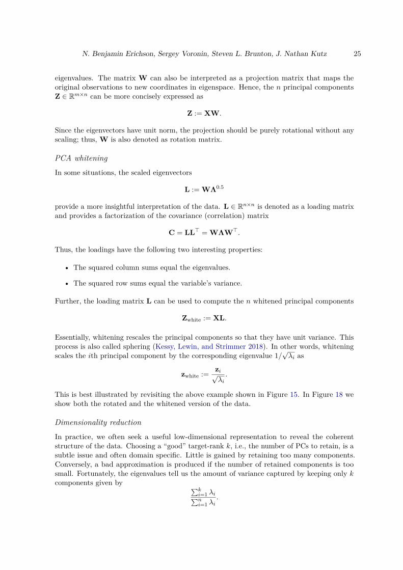
eigenvalues. The matrix W can also be interpreted as a projection matrix that maps theoriginal observations to new coordinates in eigenspace. Hence, the n principal componentsZ ∈ Rm×n can be more concisely expressed as
Z := XW.
Since the eigenvectors have unit norm, the projection should be purely rotational without anyscaling; thus, W is also denoted as rotation matrix.
PCA whitening
In some situations, the scaled eigenvectors
L := WΛ0.5
provide a more insightful interpretation of the data. L ∈ Rn×n is denoted as a loading matrixand provides a factorization of the covariance (correlation) matrix
C = LL> = WΛW>.
Thus, the loadings have the following two interesting properties:
• The squared column sums equal the eigenvalues.
• The squared row sums equal the variable’s variance.
Further, the loading matrix L can be used to compute the n whitened principal components
Zwhite := XL.
Essentially, whitening rescales the principal components so that they have unit variance. Thisprocess is also called sphering (Kessy, Lewin, and Strimmer 2018). In other words, whiteningscales the ith principal component by the corresponding eigenvalue 1/
√λi as
zwhite := zi√λi.
This is best illustrated by revisiting the above example shown in Figure 15. In Figure 18 weshow both the rotated and the whitened version of the data.
Dimensionality reduction
In practice, we often seek a useful low-dimensional representation to reveal the coherentstructure of the data. Choosing a “good” target-rank k, i.e., the number of PCs to retain, is asubtle issue and often domain specific. Little is gained by retaining too many components.Conversely, a bad approximation is produced if the number of retained components is toosmall. Fortunately, the eigenvalues tell us the amount of variance captured by keeping only kcomponents given by ∑k
i=1 λi∑ni=1 λi
.

26 Randomized Matrix Decompositions Using R
(a) Rotated data. (b) Rotated and whitened data.
Figure 18: Plot (a) shows the principal components and plot (b) shows the whitened principalcomponents. The whitened components are uncorrelated and have unit variance.
Thus, PCs corresponding to eigenvalues of small magnitude account only for a small amountof information in the data.Many different heuristics, like the scree plot and Kaiser criterion, have been proposed toidentify the optimal number of components (Jolliffe 2002). A computational intensive approachto determine the optimal number of components is via cross-validation approximations (Josseand Husson 2012), while a mathematically refined approach is the optimal hard thresholdmethod for singular values, formulated by Gavish and Donoho (2014). An interesting Bayesianapproach to estimate the intrinsic dimensionality of a high-dimensional dataset was recentlyproposed by Bouveyron, Latouche, and Mattei (2017).
4.2. Randomized algorithm
The singular value decomposition provides a computationally efficient and numerically stableapproach for computing the principal components. Specifically, the eigenvalue decompositionof the inner and outer dot product of X = UΣV> can be related to the SVD as
X>X = (VΣU>)(UΣV>) = VΣ2V>, (11a)XX> = (UΣV>)(VΣU>) = UΣ2U>. (11b)
It follows that the eigenvalues are equal to the squared singular values. Thus, we recover theeigenvalues of the sample covariance matrix C := (m− 1)−1X>X as Λ = (m− 1)−1Σ2.The left singular vectors U correspond to the eigenvectors of the outer product XX>, andthe right singular vectors V correspond to the eigenvectors of the inner product X>X. Thisallows us to define the projection (rotation) matrix W := V.Having established the connection between the singular value decomposition and principalcomponent analysis, it is straight forward to show that the principal components can becomputed as
Z := XW = UΣV>W = UΣ.
N. Benjamin Erichson, Sergey Voronin, Steven L. Brunton, J. Nathan Kutz 27
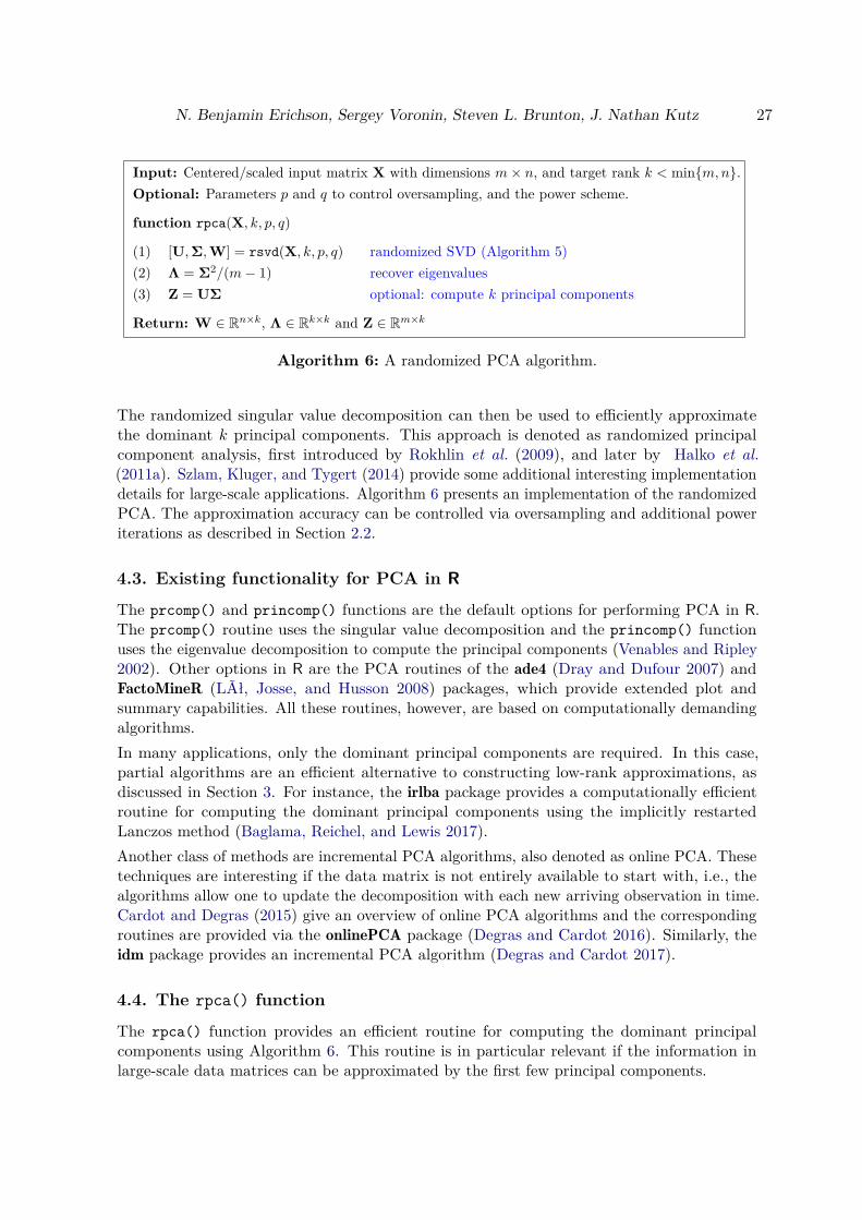
Input: Centered/scaled input matrix X with dimensions m× n, and target rank k < minm,n.Optional: Parameters p and q to control oversampling, and the power scheme.
function rpca(X, k, p, q)
(1) [U,Σ,W] = rsvd(X, k, p, q) randomized SVD (Algorithm 5)(2) Λ = Σ2/(m− 1) recover eigenvalues(3) Z = UΣ optional: compute k principal components
Return: W ∈ Rn×k, Λ ∈ Rk×k and Z ∈ Rm×k
Algorithm 6: A randomized PCA algorithm.
The randomized singular value decomposition can then be used to efficiently approximatethe dominant k principal components. This approach is denoted as randomized principalcomponent analysis, first introduced by Rokhlin et al. (2009), and later by Halko et al.(2011a). Szlam, Kluger, and Tygert (2014) provide some additional interesting implementationdetails for large-scale applications. Algorithm 6 presents an implementation of the randomizedPCA. The approximation accuracy can be controlled via oversampling and additional poweriterations as described in Section 2.2.
4.3. Existing functionality for PCA in R
The prcomp() and princomp() functions are the default options for performing PCA in R.The prcomp() routine uses the singular value decomposition and the princomp() functionuses the eigenvalue decomposition to compute the principal components (Venables and Ripley2002). Other options in R are the PCA routines of the ade4 (Dray and Dufour 2007) andFactoMineR (LÃł, Josse, and Husson 2008) packages, which provide extended plot andsummary capabilities. All these routines, however, are based on computationally demandingalgorithms.In many applications, only the dominant principal components are required. In this case,partial algorithms are an efficient alternative to constructing low-rank approximations, asdiscussed in Section 3. For instance, the irlba package provides a computationally efficientroutine for computing the dominant principal components using the implicitly restartedLanczos method (Baglama, Reichel, and Lewis 2017).Another class of methods are incremental PCA algorithms, also denoted as online PCA. Thesetechniques are interesting if the data matrix is not entirely available to start with, i.e., thealgorithms allow one to update the decomposition with each new arriving observation in time.Cardot and Degras (2015) give an overview of online PCA algorithms and the correspondingroutines are provided via the onlinePCA package (Degras and Cardot 2016). Similarly, theidm package provides an incremental PCA algorithm (Degras and Cardot 2017).
4.4. The rpca() function
The rpca() function provides an efficient routine for computing the dominant principalcomponents using Algorithm 6. This routine is in particular relevant if the information inlarge-scale data matrices can be approximated by the first few principal components.

28 Randomized Matrix Decompositions Using R
The interface of the rpca() function is similar to the prcomp() function:
rpca(A, k, center = TRUE, scale = TRUE, retx = TRUE, p = 10, q = 2)
The first mandatory argument A passes the m× n input data matrix. Note, that the analysiscan be affected if the variables have different units of measurement. In this case, scalingis required to ensure a meaningful interpretation of the components. The rpca() functioncenters and scales the input matrix by default, i.e., the analysis is based on the implicitcorrelation matrix. However, if all of the variables have same units of measurement, there isthe option to work with either the covariance or correlation matrix. In this case, the choicelargely depends on the data and the aim of the analysis. The default options can be changedvia the arguments center and scale. The second mandatory argument k sets the target rank,and it is assumed that k is smaller than the ambient dimensions of the input matrix. Theprincipal components are returned by default; otherwise the argument retx can be set toFALSE to not return the PCs. The parameters p and q are described in Section 3.6.The resulting model object is a list and contains the following components:
• rotation: n× k matrix containing the eigenvectors.• eigvals: k-dimensional vector containing the eigenvalues.• sdev: k-dimensional vector containing the standard deviations of the principal compo-
nents, i.e., the square root of the eigenvalues.• x: m× k matrix containing the principal components (rotated variables).• center, scale: the numeric centering and scalings used (if any).
Utility functions
The rpca() routine comes with methods that can be used to summarize and display the modelinformation. These are similar to the prcomp() function. The summary() function providesinformation about the explained variance, standard deviations, proportion of variance as wellas the cumulative proportion of the computed principal components. The print() functioncan be used to print the eigenvectors (principal directions). The plot() function can be usedto visualize the results, using the ggplot2 package (Wickham 2009).
4.5. PCA example: Handwritten digits
Handwritten digit recognition is a widely studied problem (Lecun, Bottou, Bengio, and Haffner1998). In the following, we use a downsampled version of the MNIST (Modified NationalInstitute of Standards and Technology) database of handwritten digits. The data are obtainedfrom http://yann.lecun.com/exdb/mnist and can be loaded from the command line:
R> data("digits", package = "rsvd")R> label <- as.factor(digits[, 1])R> digits <- digits[, 2:785]
The data matrix is of dimension 12000× 785. Each row corresponds to a digit between 0 and3. The first column is comprised of the class labels, while the following 784 columns recordthe pixel intensities for the flattened 28× 28 image patches. Figure 21a shows some of thedigits. In R the first digit can be displayed as:

N. Benjamin Erichson, Sergey Voronin, Steven L. Brunton, J. Nathan Kutz 29
0.2
0.4
0.6
0.8
0 10 20 30 40
Principal components
Cum
mula
tive
pro
port
ion
Figure 19: Cumulative proportion of the variance explained by the principal components. Thefirst 40 PCs explain about 82% of the total variation in the data.
R> digit <- matrix(digits[1, ], nrow = 28, ncol = 28)R> image(digit[, 28:1], col = gray(255:0 / 255))
The aim of principal component analysis is to find a low-dimension representation whichcaptures most of the variation in the data. PCA helps to understand the sources of variabilityin the data as well as to understand correlations between variables. The principal componentscan be used for visualization, or as features to train a classifier. A common choice is to retainthe dominant 40 principal components for classifying digits, using the k-nearest neighboralgorithm (Lecun et al. 1998). Those can be efficiently approximated using the rpca()function:
R> digits.rpca <- rpca(digits, k = 40, center = TRUE, scale = FALSE)
The target rank is defined via the argument k. By default, the data are mean centered andstandardized, i.e., the correlation matrix is implicitly computed. Here, we set scale = FALSE,since the variables have the same units of measurement, namely pixel intensities. The analysiscan be summarized using the summary() function. The screeplot function can be used tovisualize the cumulative proportion of the variance captured by the principal components:
R> ggscreeplot(digits.rpca, type = "cum")
Figure 19 shows the corresponding plot. Next, the PCs can be plotted in order to visualizethe data in low-dimensional space:
R> ggindplot(digits.rpca, groups = label, ellipse = TRUE, ind_labels = FALSE)
The so-called individual factor map, using the first and second principal component, is shownin Figure 20a. The plot helps to reveal some interesting patterns in the data. For instance, 0’sare distinct from 1’s, while 3’s share commonalities with all the other classes. Further, thecorrelation between the original variables and the PCs can be visualized:
R> ggcorplot(digits.rpca, alpha = 0.3, top.n = 10)
The correlation plot, also denoted as variables factor map, is shown in Figure 20b. It showsthe projected variables in eigenspace. This representation of the data gives some insights intothe structural relationship (correlation) between the variables and the principal components.

30 Randomized Matrix Decompositions Using R
(a) Individuals factor map. (b) Variables factor map.
Figure 20: Plotting functionality to visualize the PCs: (a) shows the individuals factor map,overlaid with ellipses for each class; (b) shows the variables factor map.
In order to quantify the quality of the dimensionality reduction, we can compute the relativeerror between the low-rank approximation and the original data. Recall, that the dominantk principal component were defined as Zk := XWk. Hence, we can approximate the inputmatrix as X ≈ ZkW>
k :
R> digits.re <- digits.rpca$x %*% t(digits.rpca$rotation)
Since the procedure has centered the data, we need to add the mean pixel values back:
R> digits.re <- sweep(digits.re, 2, digits.rpca$center, FUN = "+")
The relative error can then be computed:
R> norm(digits - digits.re, "F") / norm(digits, "F")
The relative error is approximately 32.8%. Figure 21b and 21c show the samples of thereconstructed digits using both the prcomp() and rpca() function. By visual inspection,there is virtually no noticeable difference between the deterministic and the randomizedapproximation.Runtimes and relative errors for different PCA functions in R are listed in Table 2. Therandomized algorithm is much faster than the prcomp() function, while attaining near-optimalresults. Both the dudi.pca() and PCA() functions are slower than the base prcomp() function.This is because we are using the MKL (math kernel library) accelerated R distribution MicrosoftR Open 3.4.1. The timings can vary compared to using the standard R distribution.
Handwritten digit recognition
The principal component scores can be used as features to efficiently train a classifier. Thisis because PCA assumes that the interesting information in the data are reflected by thedominant principal components. This assumption is not always valid, i.e., in some applications

N. Benjamin Erichson, Sergey Voronin, Steven L. Brunton, J. Nathan Kutz 31
Package Function Parameters Time (s) Speedup Errorbase prcomp() rank. = 40 0.56 * 0.327FactoMineR PCA() ncp = 40 0.97 0.57 0.327ade4 dudi.pca() nf = 40 0.91 0.61 0.327irlba prcomp_irlba() n = 40 0.47 1.2 0.327rsvd rpca() k = 40 0.37 1.5 0.328
Table 2: Summary of the computational performance of different PCA functions.
(a) Handwritten digits. (b) Deterministic. (c) Randomized.
Figure 21: Handwritten digits, and its low-rank approximations using k = 40 components.
it can be the case that the variance corresponds to noise rather than to the underlying signal.The question is, how good are the randomized principal components suited for this task? Inthe following, we use a simple k-nearest neighbor (kNN) algorithm to classify handwrittendigits in order to compare the performance. The idea of kNN is to find the closest point (orset of points) to a given target point (Hastie, Tibshirani, and Friedman 2009). There aretwo reasons to use PCA for dimensionality reduction: (a) kNN is known to perform poorlyin high-dimensional space, due to the “curse of dimensionality” (Donoho 2000); (b) kNN iscomputational expensive when high-dimensional data points are used for training.First, we split the dataset into a training and a test set using the caret package (Kuhn 2008).We aim to create a balanced split of the dataset, using about 80% of the data for training:
R> library("caret")R> trainIndex <- createDataPartition(label, p = 0.8, list = FALSE)
We then compute the dominant k = 40 randomized principal components of the training set:
R> train.rpca <- rpca(digits[trainIndex, ], k = 40, scale = FALSE)
We can use the predict() function to rotate the test set into low-dimensional space:
R> test.x <- predict(train.rpca, digits[-trainIndex, ])
The base class package provides a kNN algorithm, which we use for classification:
R> library("class")R> knn.1 <- knn(train.rpca$x, test.x, label[trainIndex], k = 1)
32 Randomized Matrix Decompositions Using R
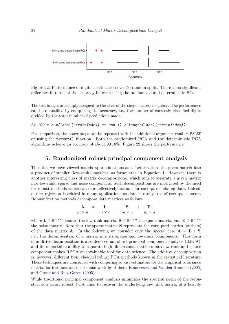
kNN using randomized PCs
kNN using deterministic PCs
98.9 99.1 99.3
Accuracy
Figure 22: Performance of digits classification over 50 random splits. There is no significantdifference in terms of the accuracy between using the randomized and deterministic PCs.
The test images are simply assigned to the class of the single nearest neighbor. The performancecan be quantified by computing the accuracy, i.e., the number of correctly classified digitsdivided by the total number of predictions made:
R> 100 * sum(label[-trainIndex] == knn.1) / length(label[-trainIndex])
For comparison, the above steps can be repeated with the additional argument rand = FALSEor using the prcomp() function. Both the randomized PCA and the deterministic PCAalgorithms achieve an accuracy of about 99.18%. Figure 22 shows the performance.
5. Randomized robust principal component analysisThus far, we have viewed matrix approximations as a factorization of a given matrix intoa product of smaller (low-rank) matrices, as formulated in Equation 1. However, there isanother interesting class of matrix decompositions, which aim to separate a given matrixinto low-rank, sparse and noise components. Such decompositions are motivated by the needfor robust methods which can more effectively account for corrupt or missing data. Indeed,outlier rejection is critical in many applications as data is rarely free of corrupt elements.Robustification methods decompose data matrices as follows:
A ≈ L + S + E,m× n m× n m× n m× n
where L ∈ Rm×n denotes the low-rank matrix, S ∈ Rm×n the sparse matrix, and E ∈ Rm×n
the noise matrix. Note that the sparse matrix S represents the corrupted entries (outliers)of the data matrix A. In the following we consider only the special case A = L + S,i.e., the decomposition of a matrix into its sparse and low-rank components. This formof additive decomposition is also denoted as robust principal component analysis (RPCA),and its remarkable ability to separate high-dimensional matrices into low-rank and sparsecomponent makes RPCA an invaluable tool for data science. The additive decompositionis, however, different from classical robust PCA methods known in the statistical literature.These techniques are concerned with computing robust estimators for the empirical covariancematrix, for instance, see the seminal work by Hubert, Rousseeuw, and Vanden Branden (2005)and Croux and Ruiz-Gazen (2005).While traditional principal component analysis minimizes the spectral norm of the recon-struction error, robust PCA aims to recover the underlying low-rank matrix of a heavily

N. Benjamin Erichson, Sergey Voronin, Steven L. Brunton, J. Nathan Kutz 33
corrupted input matrix. Candès, Li, Ma, and Wright (2011) proved that it is possible toexactly separate such a data matrix A ∈ Rm×n into both its low-rank and sparse components,under rather broad assumptions. This is achieved by solving a convenient convex optimizationproblem called principal component pursuit (PCP). The objective is to minimize a weightedcombination of the nuclear norm ‖ · ‖∗ :=
∑i σi and the `1 norm ‖ · ‖1 :=
∑ij |mij | as
minL,S‖L‖∗ + λ‖S‖1 subject to A− L− S = 0,
where λ is an arbitrary balance parameter which puts some weight on the sparse error termin the cost function. Typically λ is chosen to be λ = maxn,m−0.5. The PCP concept ismathematically sound, and has been applied successfully to many applications like videosurveillance and face recognition (Wright, Ganesh, Rao, Peng, and Ma 2009). Robust PCA isparticular relevant if the underlying model of the data naturally features a low-rank subspacethat is polluted with sparse components. The concept of matrix recovery can also be extendedto the important problem of matrix completion.The biggest challenge for robust PCA is computational efficiency, especially given the iterativenature of the optimization required. Bouwmans, Sobral, Javed, Jung, and Zahzah (2016) haveidentified more than 30 related algorithms to the original PCP approach, aiming to overcomethe computational complexity, and to generalize the original algorithm.
5.1. The inexact augmented Lagrange multiplier method
A popular choice to compute RPCA, due to its favorable computational properties, is theinexact augmented Lagrange multiplier (IALM) method (Lin, Chen, and Ma 2011). Thismethod formulates the following Lagrangian function
L(L,S,Z, µ) = ‖L‖∗ + λ‖S‖1 + 〈Z,A− L− S〉+ µ
2 ‖A− L− S‖2F , (12)
where µ and λ are positive scalars, and Z the Lagrange multiplier. Further, 〈·, ·〉 is defined as〈A,B〉 := trace(A>B). The method of augmented Lagrange multipliers can be used to solvethe optimization problem (Bertsekas 1999). Lin et al. (2011) have proposed both an exact andinexact algorithm to solve Equation 12. Here, we advocate the latter approach. Specifically,the inexact algorithm avoids solving the problem
Li+1,Ei+1 = argminL,E
L(L,E,Zi, µk),
by alternately solving the following two sub-problems at step i:
Li+1 = argminLL(L,Ei,Zi, µk),
andEi+1 = argmin
EL(Li+1,E,Zi, µk).
For details, we refer the reader to Lin et al. (2011).
5.2. Randomized algorithm
The singular value decomposition is the workhorse algorithm behind the IALM method. Thus,the computational costs can become intractable for “big” datasets. However, randomized SVD

34 Randomized Matrix Decompositions Using R
Input: Input matrix A with dimensions m× n, and λ to put weight on the sparse error term.Optional: Parameters p and q to control oversampling, and the power scheme.
function rrpca(A, λ, p, q)
(1) k = 2 initialize target rank(2) µ = 1.25 · ‖A‖2 initialize µ(3) Z = A · dual_norm(A)−1 initialize Lagrange multiplier(4) S = matrix(0,m, n) initialize sparse matrix
(5) repeat(6) [U,Σ,V] = rsvd(A− S + Z · µ−1, k, p, q) randomized SVD using Algorithm 5(7) k, l = predict_rank(Σ, µ−1) predicted rank, and updated target rank(8) Σl = soft_thres(diag(Σ)(1 : l), µ−1) soft threshold top l singular values(9) L = U(:, 1 : l)ΣlV(:, 1 : l)> update low-rank matrix(10) S = soft_thres(A− L + Z · µ−1, λ · µ−1) update sparse matrix via soft thresholding(11) Z = Z + (A− L− S) · µ update Lagrange multiplier(12) update µ(13) until some convergence criterion is reached
Return: L ∈ Rm×n, and S ∈ Rm×n
Remark 3. Lin et al. (2011) provide details on how to predict the rank in Step (6).Remark 4. Our randomized RPCA algorithm automatically switches from the randomizedSVD to the deterministic SVD, if the target rank is predicted to be k > minm,n/4.
Algorithm 7: A randomized robust PCA algorithm.
can be used to substantially ease the computational burden of the IALM method. Algorithm 7outlines the randomized implementation.
5.3. Existing functionality for robust PCA in ROnly few R packages provide robust PCA routines. For comparison, we consider the rpcapackage (Sykulski 2015). The provided RPCA function implements the algorithm describedby Candès et al. (2011). This algorithm is highly accurate. However, a large number ofiterations is required for convergence.
5.4. The rrpca() function
The rrpca() function implements the inexact augmented Lagrange multiplier method. Theinterface of the rrpca() function takes the form of:
rrpca(A, lambda = NULL, maxiter = 50, tol = 1.0e-5, p = 10, q = 2,trace = FALSE, rand = TRUE)
The first mandatory argument A passes the m× n input data matrix. The second argumentlambda is used to put some weight on the sparse error term in the cost function. By default λ

N. Benjamin Erichson, Sergey Voronin, Steven L. Brunton, J. Nathan Kutz 35
is set to λ = maxn,m−0.5. The next two parameters maxiter, and tol are used to controlthe stopping criterion of the algorithm. The routine stops either if a specified maximal numberof iterations, or if a certain tolerance level is reached. The parameters p and q are described inSection 2. The argument rand can be used to switch between the deterministic and randomizedalgorithms. By default the randomized algorithm is selected (i.e., the randomized SVD is used).Setting this argument rand = FALSE selects the deterministic algorithm (i.e., the deterministicSVD is used). To print out progress information, the argument trace can be set TRUE.The resulting model object is a list and contains the following components:
• L: m× n matrix containing the low-rank component.• S: m× n matrix containing the sparse component.
5.5. Robust PCA example: Grossly corrupted handwritten digits
To demonstrate the randomized robust PCA algorithm, we consider a grossly corrupted subsetof the handwritten digits dataset. We first extract a subset comprising only twos:
R> data("digits", package = "rsvd")R> two <- subset(digits[, 2:785], digits[, 1] == 2)
Then, we corrupt the data using salt and pepper noise, i.e., we draw i.i.d. uniform entries inthe interval [0, 255] and sparsify the matrix so that about 10% nonzero elements are retained:
R> m <- nrow(two); n <- ncol(two)R> S <- matrix(runif(m * n, 0, 255), nrow = m, ncol = n)R> S <- S * matrix(rbinom(m*n, size = 1, prob = 0.1), nrow = m, ncol = n)
The digits are then corrupted as follows:
R> two_noisy <- two + SR> two_noisy <- ifelse(two_noisy > 255, 255, two_noisy)
Note, the last line ensures that the pixel intensities remain in the interval [0, 255]. Samples ofthe corrupted digits are shown in Figure 23a. Robust PCA is now used for matrix recovery(denoising) by separating the data into a low-rank and sparse component:
R> two.rrpca <- rrpca(two_noisy, trace = TRUE, rand = TRUE)
Figure 23c and 23d shows samples of the low-rank component L and the sparse component S.For comparison, Figure 23b shows samples of the low-rank component which are computedusing the deterministic routine (rand = FALSE).Table 3 summarizes the computational results. The randomized routine does not show acomputational advantage in this case. The reasons are twofold. First, the dataset requiresa relatively large target rank to approximate the data accurately, i.e., in this example thepredicted rank-k of the IALM algorithm for the final iteration is 232. Secondly, the datamatrix is tall and thin (i.e., the ratio of rows to columns is large). For both of theses reasons,the performance of the deterministic algorithm remains competitive. The advantage of therandomized algorithms becomes pronounced for higher-dimensional problems which featurelow-rank structure.

36 Randomized Matrix Decompositions Using R
(a) Noisy digits. (b) Deterministic L. (c) Randomized L. (d) Randomized S.
Figure 23: Separation of noisy handwritten digits into a low-rank and a sparse component.
Package Function Parameters Time (s) Speedup Error Iterationsrpca rpca() max.iter = 50 11.88 * 0.265 50rsvd rrpca() rand = FALSE 6.33 1.8 0.328 27rsvd rrpca() rand = TRUE 5.56 2.1 0.329 27
Table 3: Summary of the computational performance of different RPCA functions.
It appears that the rpca() routine of the rpca package is more accurate, while computationallyless attractive (the algorithm converges slowly). However, using the relative error for comparingthe algorithms might be misleading since we do not know the ground truth. The relativeerror is computed using the original data as baseline, which contains some perturbations itself.Clearly, the advocated IALM algorithm removes not only the salt and paper noise, but alsoshadows, specularities, and saturations from the digits. This seems to be favorable, yet itleads to a larger relative error. Thus, to better compare the algorithms we perform a smallsimulation study using synthetic data. By superimposing a low-rank matrix with a sparsecomponent, the ground truth is known. First, the low-rank component is generated:
R> m <- 300; n <- 300; k <- 5R> L1 <- matrix(rnorm(m * k), nrow = m, ncol = k)R> L2 <- matrix(rnorm(n * k), nrow = k, ncol = n)R> L <- L1 %*% L2
The sparse component with about 20% nonzero i.i.d. uniform entries in the interval [−500, 500]is generated from:
R> S <- matrix(runif(m * n, -500, 500), nrow = m, ncol = n)R> S <- S * matrix(rbinom(m * n, size = 1, prob = 0.2), nrow = m, ncol = n)
The data matrix is then constructed by superimposing the low-rank and sparse components:
R> A <- L + S

N. Benjamin Erichson, Sergey Voronin, Steven L. Brunton, J. Nathan Kutz 37
Deterministic RPCA
Randomized RPCA
rpca::RPCA with max iterations set to 50
rpca::RPCA with max iterations set to 100
0.00025 0.00050 0.00075 0.00100
Accuracy
Figure 24: Matrix recovery performance of different RPCA algorithms.
Figure 24 shows the performance of the RPCA algorithms over 50 runs. Both the randomizedand deterministic routines provided by the rsvd package show a better performance than therpca package, when the maximum number of iterations is set to 50. In addition, we show theperformance after 100 iterations for the RPCA algorithms from the rpca package.
6. Additional functionalityPrincipal components analysis seeks a set of new components which are formed as weightedlinear combinations of the input data. This approach allows one to efficiently approximateand summarize the data, however, interpretation of the resulting components can be difficult.For instance, in a high-dimensional data setting it is cumbersome to interpret the largenumber of weights (loadings) required to form the components. While in many applicationsthe eigenvectors have distinct meanings, the orthogonality constraints may not be physicalmeaningful in other problems. Thus, it is plausible to look for alternative factorizationswhich may not provide an optimal rank-k approximation, but which may preserve usefulproperties of the input matrix, such as sparsity and non-negativity as well as allowing foreasier interpretation of its components. Such properties may be found in the CUR and theinterpolative decompositions (ID), which are both tools for computing low-rank approximations.
6.1. Randomized CUR decomposition
Mahoney and Drineas (2009) introduced the CUR matrix decomposition, as an interest-ing alternative to traditional approximation techniques such as SVD and PCA. The CURdecomposition admits a factorization of the form
A ≈ C U R,m× n m× k k × k k × n
where the components of the matrix C ∈ Rm×k and R ∈ Rk×n are formed by small subsets ofactual columns and rows, respectively. The matrix U ∈ Rk×k is formed so that ‖A−CUR‖Fis small. The CUR factorization is illustrated in Figure 25.

38 Randomized Matrix Decompositions Using R
=
Figure 25: Schematic of the rank-k CUR decomposition of an m× n matrix. The componentsare formed by small subsets of actual columns and rows of the input matrix.
The low-rank factor matrices C and R are interpretable, since their components maintain theoriginal structure of the data. This allows one to fully leverage any field-specific knowledgeabout the data, i.e., experts have often a clear understanding about the actual meaning ofcertain columns and rows. However, the CUR decomposition is not unique, and different com-putational strategies lead to different subsets of columns and rows, for instance, see Mahoneyand Drineas (2009) and Boutsidis and Woodruff (2017). Thus, the practical meaning of theselected rows and columns should always be carefully examined depending on the problemand its objective.Note, that the rank-k SVD (Ak = UkΣkV>k ) of a general m× n matrix A yields an optimalapproximation of rank k to A, in the sense that ‖A − Ak‖ ≤ ‖A −Mk‖ for any rank kmatrix Mk, both in the operator (spectral) and Frobenius norms. However, if A is a sparsematrix, the m× k and n× k factors Uk and Vk are typically dense. Even though the low-rankSVD is optimal for a given rank k, the choice of rank may be limited to relatively low valueswith respect to min(m,n) for sparse matrices, in order to achieve any useful compressionratios. Of course, the usefulness of the SVD is not limited to compression; but the utilityof a low-rank approximation is greatly reduced once the storage size of the factors exceedsthat of the original matrix. The CUR decomposition provides an interesting alternative forcompression, since its components preserve sparsity.The rCUR package provides an implementation in R (Bodor, Csabai, Mahoney, and Solymosi2012). The rsvd package implements both the deterministic and randomized CUR decompo-sition, following the work by Voronin and Martinsson (2017). Specifically, the interpolativedecomposition is used as an algorithmic tool to form the factor matrices C and R. Algorithm 8outlines the computational steps of the rcur() routine as implemented in the rsvd package.
6.2. The rcur() function
The rcur() function provides the option to compute both the deterministic and the randomizedCUR decomposition via Algorithm 8. The interface of the rcur() function is as follows:
rcur(A, k, p = 10, q = 0, idx_only = FALSE, rand = TRUE)
The first mandatory argument A passes the m× n input data matrix. The second mandatoryargument k sets the target rank, which is required to be k < minm,n. The parametersp and q are described in Section 2. The argument rand can be used to switch between thedeterministic and the randomized algorithm. The latter is used by default, and is more efficient
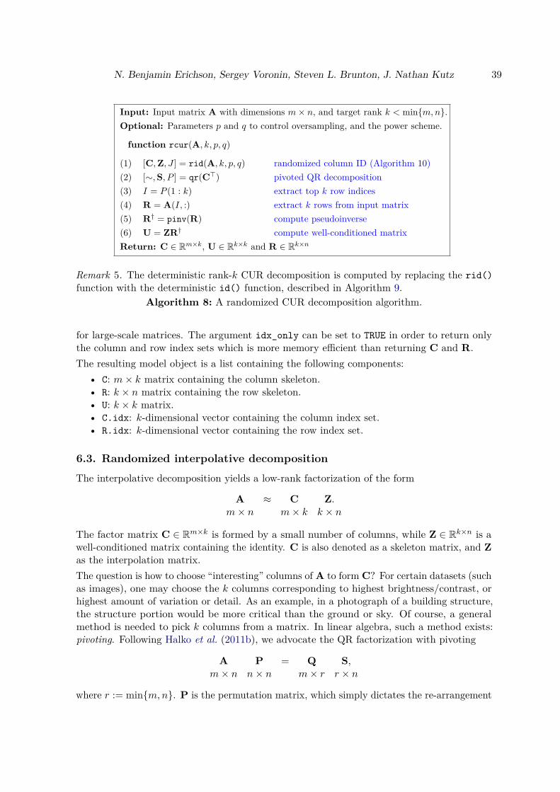
N. Benjamin Erichson, Sergey Voronin, Steven L. Brunton, J. Nathan Kutz 39
Input: Input matrix A with dimensions m× n, and target rank k < minm,n.Optional: Parameters p and q to control oversampling, and the power scheme.
function rcur(A, k, p, q)
(1) [C,Z, J ] = rid(A, k, p, q) randomized column ID (Algorithm 10)(2) [∼,S, P ] = qr(C>) pivoted QR decomposition(3) I = P (1 : k) extract top k row indices(4) R = A(I, :) extract k rows from input matrix(5) R† = pinv(R) compute pseudoinverse(6) U = ZR† compute well-conditioned matrixReturn: C ∈ Rm×k, U ∈ Rk×k and R ∈ Rk×n
Remark 5. The deterministic rank-k CUR decomposition is computed by replacing the rid()function with the deterministic id() function, described in Algorithm 9.
Algorithm 8: A randomized CUR decomposition algorithm.
for large-scale matrices. The argument idx_only can be set to TRUE in order to return onlythe column and row index sets which is more memory efficient than returning C and R.The resulting model object is a list containing the following components:
• C: m× k matrix containing the column skeleton.• R: k × n matrix containing the row skeleton.• U: k × k matrix.• C.idx: k-dimensional vector containing the column index set.• R.idx: k-dimensional vector containing the row index set.
6.3. Randomized interpolative decomposition
The interpolative decomposition yields a low-rank factorization of the form
A ≈ C Z.m× n m× k k × n
The factor matrix C ∈ Rm×k is formed by a small number of columns, while Z ∈ Rk×n is awell-conditioned matrix containing the identity. C is also denoted as a skeleton matrix, and Zas the interpolation matrix.The question is how to choose “interesting” columns of A to form C? For certain datasets (suchas images), one may choose the k columns corresponding to highest brightness/contrast, orhighest amount of variation or detail. As an example, in a photograph of a building structure,the structure portion would be more critical than the ground or sky. Of course, a generalmethod is needed to pick k columns from a matrix. In linear algebra, such a method exists:pivoting. Following Halko et al. (2011b), we advocate the QR factorization with pivoting
A P = Q S,m× n n× n m× r r × n
where r := minm,n. P is the permutation matrix, which simply dictates the re-arrangement

40 Randomized Matrix Decompositions Using R
Input: Input matrix A with dimensions m× n, and target rank k < minm,n.
function id(A, k)
(1) [∼,S, P ] = qr(A) pivoted QR decomposition(2) S† = pinv(S(1 : k, 1 : k)) compute pseudoinverse(3) T = S†S(1 : k, (k + 1) : n) compute expansions coefficients(4) Z = matrix(0, k, n) create empty k × n matrix(5) Z(:, P ) = cbind(diag(k),T) ordered expansions coefficients, using pivots P(6) J = P (1 : k) extract top k column indices from pivots(7) C = A(:, J) extract k columns from input matrix
Return: C ∈ Rm×k, Z ∈ Rk×n, and J ∈ Nk
Remark 6. The QR decomposition returns the permutation matrix P in form of a vectorP ∈ Rn. This vector contains the indices such that P = I(:, P ), where I ∈ Rn×n denotes theidentity matrix. Thus, J is comprised of the k dominant pivots.
Algorithm 9: An interpolative decomposition algorithm.
of the columns of A. The matrix Q has orthonormal columns, and S is upper triangular.1Because, the pivoted QR decomposition is an iterative algorithm, it can be stopped after kiterations to obtain only the k dominant pivots. Thus, the column subset used to form C issimply based on the pivoting strategy used in the QR factorization. The computational stepsrequired to compute the ID are outlined in Algorithm 9.The procedure can be considerably accelerated by means of randomization. Specifically, wecan first compute the randomized QB decomposition via Algorithm 4. Then, the smallermatrix B is used to compute the ID decomposition. The computational steps are outlinedin Algorithm 10. For a detailed discussion, and theoretical results we refer to Voronin andMartinsson (2015), and Voronin and Martinsson (2017). Therein, it is also described how thefactor matrix Z can be efficiently constructed. Note, however, that our algorithm differs fromthe implementation by Voronin and Martinsson (2015). We compute the ID based on thematrix B (obtained as described in Section 2). In our experiments, this approach shows to bemore accurate, while slightly more computational demanding.
6.4. The rid() function
The rid() function provides the option to compute both the deterministic and the randomizedinterpolative decomposition via Algorithms 9 and 10. The interface of the rid() functiontakes the following functional form:
rid(A, k, mode = "col", p = 10, q = 0, idx_only = FALSE, rand = TRUE)
The first mandatory argument A passes the m× n input data matrix. The second mandatoryargument k sets the desired target rank, which is required to be k < minm,n. The argumentmode = c("col", "row") determines whether the column or row ID should be computed.
1Here, we denote the upper triangular matrix as S, since R is occupied by the CUR decomposition.

N. Benjamin Erichson, Sergey Voronin, Steven L. Brunton, J. Nathan Kutz 41
Input: Input matrix A with dimensions m× n, and target rank k < minm,n.Optional: Parameters p and q to control oversampling and the power scheme.
function rid(A, k, p, q)
(1) [∼,B] = rqb(A, k, q, p) randomized QB decomposition via Algorithm 4(2) [∼,Z, J ] = id(B, k) column ID via Algorithm 9(3) C = A(:, J) extract k columns from input matrix
Return: C ∈ Rm×k, V ∈ Rk×n, and J ∈ Nk
Remark 7. The row ID can be computed by transposing the input matrix, i.e., A>.Algorithm 10: A randomized interpolative decomposition algorithm.
The parameters p and q are described in Section 2. The argument rand can be used to switchbetween the deterministic and randomized algorithms. By default the randomized algorithmis selected, and setting this argument rand = FALSE selects the deterministic algorithm.The resulting model object is a list and contains the following components:
• C: m× k matrix containing the column skeleton, if mode = "col".• R: k × n matrix containing the row skeleton, if mode = "row".• Z: k × n or m× k matrix (depending on mode), which is well-conditioned.• idx: k-dimensional vector containing the column or row index set.
7. ConclusionDimensionality reduction and the related concept of low-rank matrix approximations arefundamental algorithmic tools in machine learning and computational statistics. However, high-dimensional data pose a growing computational challenge for traditional matrix algorithms. Infact, the exponential growth rate of data is far outstripping advances in computational power,even of modern computational architectures. Thus, in the era of “big data”, the moderncomputational paradigm of randomized methods for linear algebra provides an attractivemethod for scalable, tractable computations. The price to pay is the trade-off between theapproximation accuracy and computational costs. In fact, randomized methods are highlyscalable, and can be used to tackle problems which are infeasible otherwise. The differentflavors of both deterministic and randomized methods are illustrated in Figure 26. Thus,randomized algorithms should be the default choice for applications which involve low-rankmatrices and do not require approximations with full double precision.Certainly, the randomized singular value decomposition is the most prominent and ubiquitousrandomized algorithm. This algorithm comes with strong theoretical error bounds, andthe approximation quality can be controlled via oversampling, and power iterations. Thecomputational advantage can be substantial compared to other SVD routines in R, providedthe target rank k is relatively small. While the performance of randomized methods depends onthe actual shape of the matrix, we can state (as a rule of thumb) that significant computationalspeedups are achieved if the target rank k is at least 3–6 times smaller than the ambientdimensions of the measurement space. The speedup for tall and thin matrices is in general
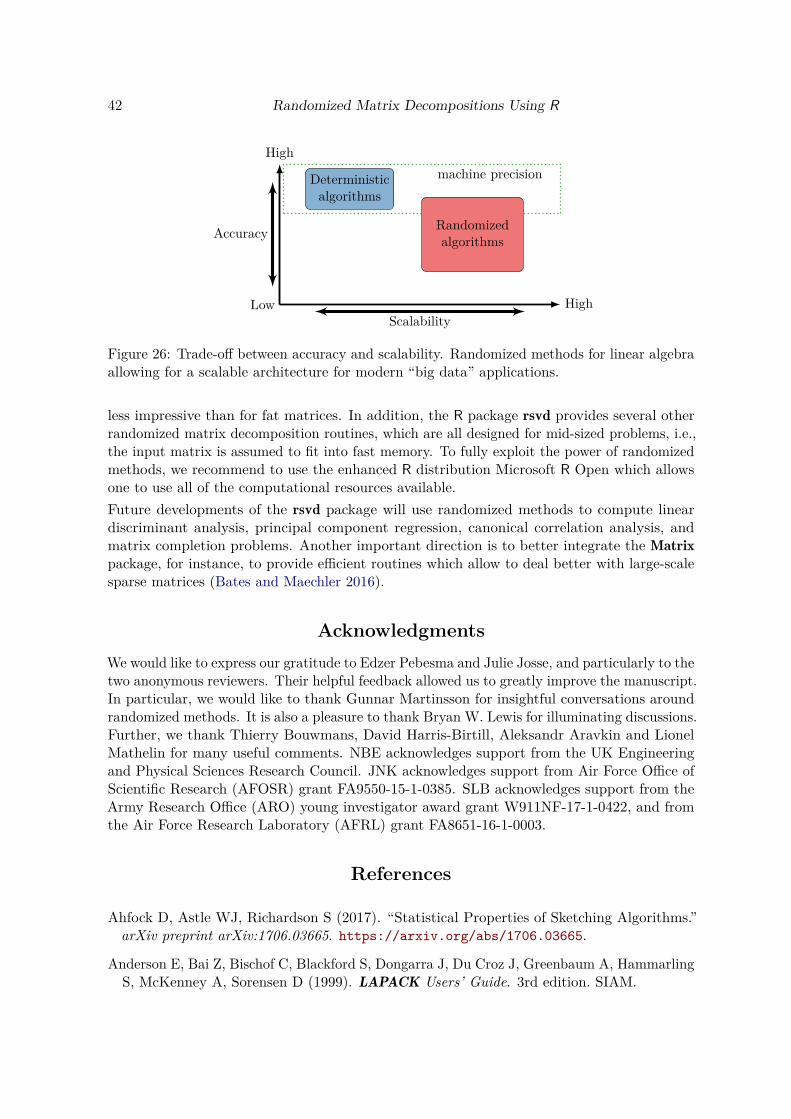
42 Randomized Matrix Decompositions Using R
Low
High
High
Accuracy
Scalability
machine precisionDeterministicalgorithms
Randomizedalgorithms
Figure 26: Trade-off between accuracy and scalability. Randomized methods for linear algebraallowing for a scalable architecture for modern “big data” applications.
less impressive than for fat matrices. In addition, the R package rsvd provides several otherrandomized matrix decomposition routines, which are all designed for mid-sized problems, i.e.,the input matrix is assumed to fit into fast memory. To fully exploit the power of randomizedmethods, we recommend to use the enhanced R distribution Microsoft R Open which allowsone to use all of the computational resources available.Future developments of the rsvd package will use randomized methods to compute lineardiscriminant analysis, principal component regression, canonical correlation analysis, andmatrix completion problems. Another important direction is to better integrate the Matrixpackage, for instance, to provide efficient routines which allow to deal better with large-scalesparse matrices (Bates and Maechler 2016).
AcknowledgmentsWe would like to express our gratitude to Edzer Pebesma and Julie Josse, and particularly to thetwo anonymous reviewers. Their helpful feedback allowed us to greatly improve the manuscript.In particular, we would like to thank Gunnar Martinsson for insightful conversations aroundrandomized methods. It is also a pleasure to thank Bryan W. Lewis for illuminating discussions.Further, we thank Thierry Bouwmans, David Harris-Birtill, Aleksandr Aravkin and LionelMathelin for many useful comments. NBE acknowledges support from the UK Engineeringand Physical Sciences Research Council. JNK acknowledges support from Air Force Office ofScientific Research (AFOSR) grant FA9550-15-1-0385. SLB acknowledges support from theArmy Research Office (ARO) young investigator award grant W911NF-17-1-0422, and fromthe Air Force Research Laboratory (AFRL) grant FA8651-16-1-0003.
References
Ahfock D, Astle WJ, Richardson S (2017). “Statistical Properties of Sketching Algorithms.”arXiv preprint arXiv:1706.03665. https://arxiv.org/abs/1706.03665.
Anderson E, Bai Z, Bischof C, Blackford S, Dongarra J, Du Croz J, Greenbaum A, HammarlingS, McKenney A, Sorensen D (1999). LAPACK Users’ Guide. 3rd edition. SIAM.

N. Benjamin Erichson, Sergey Voronin, Steven L. Brunton, J. Nathan Kutz 43
Baglama J, Reichel L (2005). “Augmented Implicitly Restarted Lanczos BidiagonalizationMethods.” SIAM Journal on Scientific Computing, 27(1), 19–42.
Baglama J, Reichel L, Lewis BW (2017). irlba: Fast Truncated Singular Value Decompositionand Principal Components Analysis for Large Dense and Sparse Matrices. R packageversion 2.2.1, URL https://CRAN.R-project.org/package=irlba.
Bates D, Maechler M (2016). Matrix: Sparse and Dense Matrix Classes and Methods. R packageversion 1.2-6, URL https://CRAN.R-project.org/package=Matrix.
Bertsekas DP (1999). Nonlinear programming. Athena scientific Belmont.
Bodor A, Csabai I, Mahoney MW, Solymosi N (2012). “rCUR: An R Package for CUR MatrixDecomposition.” BMC Bioinformatics, 13(1), 103.
Boutsidis C, Woodruff DP (2017). “Optimal CUR Matrix Decompositions.” SIAM Journal onComputing, 46(2), 543–589.
Bouveyron C, Latouche P, Mattei PA (2017). “Exact Dimensionality Selection for BayesianPCA.” arXiv preprint arXiv:1703.02834. https://arxiv.org/abs/1703.02834.
Bouwmans T, Sobral A, Javed S, Jung SK, Zahzah EH (2016). “Decomposition into Low-Rank Plus Additive Matrices for Background/Foreground Separation: A Review for aComparative Evaluation with a Large-Scale Dataset.” Computer Science Review, pp. 1–71.doi:10.1016/j.cosrev.2016.11.001.
Burges CJ (2010). “Dimension Reduction: A Guided Tour.” Foundations and Trends inMachine Learning, 2(4), 275–365.
Calvetti D, Reichel L, Sorensen DC (1994). “An Implicitly Restarted Lanczos Method forLarge Symmetric Eigenvalue Problems.” Electronic Transactions on Numerical Analysis,2(1), 21.
Candès EJ, Li X, Ma Y, Wright J (2011). “Robust Principal Component Analysis?” Journalof the ACM, 58(3), 1–37. doi:10.1145/1970392.1970395.
Cardot H, Degras D (2015). “Online Principal Component Analysis in High Dimension: WhichAlgorithm to Choose?” arXiv preprint arXiv:1511.03688.
Cipra BA (2000). “The Best of the 20th Century: Editors Name Top 10 Algorithms.” SIAMnews, 33(4), 1–2.
Croux C, Ruiz-Gazen A (2005). “High Breakdown Estimators for Principal Components: TheProjection-Pursuit Approach Revisited.” Journal of Multivariate Analysis, 95(1), 206–226.
Cunningham JP, Ghahramani Z (2015). “Linear Dimensionality Reduction: Survey, Insights,and Generalizations.” Journal of Machine Learning Research, 16, 2859–2900.
Degras D, Cardot H (2016). onlinePCA: Online Principal Component Analysis. R packageversion 1.3.1, URL https://cran.r-project.org/package=onlinePCA.
Degras D, Cardot H (2017). idm: Incremental Decomposition Methods. R package version 1.8.1,URL https://cran.r-project.org/package=idm.

44 Randomized Matrix Decompositions Using R
Demmel J (1997). Applied Numerical Linear Algebra. SIAM.
Donoho DL (2000). “High-Dimensional Data Analysis: The Curses and Blessings of Dimen-sionality.” AMS Math Challenges Lecture, pp. 1–32.
Dray S, Dufour A (2007). “The ade4 Package: Implementing the Duality Diagram forEcologists.” Journal of Statistical Software, 22(4), 1–20.
Drineas P, Mahoney MW (2016). “RandNLA: Randomized Numerical Linear Algebra.”Communications of the ACM, 59, 80–90.
Duersch JA, Gu M (2017). “Randomized QR with Column Pivoting.” SIAM Journal onScientific Computing, 39(4), C263–C291. doi:10.1137/15M1044680.
Eckart C, Young G (1936). “The Approximation of one Matrix by Another of Lower Rank.”Psychometrika, 1, 211–218.
Erichson NB, Brunton SL, Kutz JN (2017). “Randomized Dynamic Mode Decomposition.”arXiv preprint arXiv:1702.02912.
Frieze A, Kannan R, Vempala S (2004). “Fast Monte-Carlo Algorithms for Finding Low-RankApproximations.” Journal of the ACM, 51(6), 1025–1041.
Gavish M, Donoho DL (2014). “The Optimal Hard Threshold for Singular Values is 4/√
3.”IEEE Transactions on Information Theory, 60(8), 5040–5053.
Golub G, Kahan W (1965). “Calculating the Singular Values and Pseudo-Inverse of a Matrix.”SIAM, Series B: Numerical Analysis, 2(2), 205–224.
Golub GH, Reinsch C (1970). “Singular Value Decomposition and Least Squares Solutions.”Numerische Mathematik, 14, 403–420.
Golub GH, Van Loan CF (1996). Matrix Computations. 3 edition. Johns Hopkins UniversityPress.
Gu M (2015). “Subspace Iteration Randomization and Singular Value Problems.” SIAMJournal on Scientific Computing, 37(3), 1139–1173. doi:10.1137/130938700.
Halko N, Martinsson PG, Shkolnisky Y, Tygert M (2011a). “An Algorithm for the PrincipalComponent Analysis of Large Data Sets.” SIAM Journal on Scientific Computing, 33,2580–2594.
Halko N, Martinsson PG, Tropp JA (2011b). “Finding Structure with Randomness: Proba-bilistic Algorithms for Constructing Approximate Matrix Decompositions.” SIAM Review,53(2), 217–288. doi:10.1137/090771806.
Hastie T, Tibshirani R, Friedman J (2009). The Elements of Statistical Learning: Data Mining,Inference, and Prediction. Springer Series in Statistics, 2nd edition. Springer-Verlag.
Hotelling H (1933). “Analysis of a Complex of Statistical Variables into Principal Components.”Journal of Educational Psychology, 24(6), 417.

N. Benjamin Erichson, Sergey Voronin, Steven L. Brunton, J. Nathan Kutz 45
Hubert M, Rousseeuw PJ, Vanden Branden K (2005). “ROBPCA: A New Approach to RobustPrincipal Component Analysis.” Technometrics, 47(1), 64–79.
Johnson WB, Lindenstrauss J (1984). “Extensions of Lipschitz Mappings into a Hilbert Space.”Contemporary mathematics, 26(189-206), 1.
Jolliffe I (2002). Principal Component Analysis. Springer Series in Statistics, 2nd edition.Springer-Verlag.
Josse J, Husson F (2012). “Selecting the Number of Components in Principal ComponentAnalysis using Cross-Validation Approximations.” Computational Statistics & Data Analysis,56(6), 1869–1879.
Kessy A, Lewin A, Strimmer K (2018). “Optimal Whitening and Decorrelation.” The AmericanStatistician, 0(0), 1–6. doi:10.1080/00031305.2016.1277159.
Korobeynikov A, Larsen RM (2016). svd: Interfaces to Various State-of-Art SVD andEigensolvers. R package version 0.4, URL https://CRAN.R-project.org/package=svd.
Kuhn M (2008). “Caret package.” Journal of Statistical Software, 28(5), 1–26.
Larsen RM (1998). “Lanczos Bidiagonalization with Partial Reorthogonalization.” DAIMIReport Series, 27, 1–101.
Lecun Y, Bottou L, Bengio Y, Haffner P (1998). “Gradient-Based Learning Applied toDocument Recognition.” Proceedings of the IEEE, 86(11), 2278–2324. doi:10.1109/5.726791.
Lehoucq R, Sorensen D, Yang C (1998). ARPACK Users’ Guide. SIAM.
Li P, Hastie TJ, Church KW (2006). “Very sparse random projections.” In Proceedings of the12th ACM SIGKDD international conference on Knowledge discovery and data mining, pp.287–296. ACM.
Liberty E (2013). “Simple and Deterministic Matrix Sketching.” In Proceedings of the 19thACM SIGKDD International Conference on Knowledge Discovery and Data Mining, pp.581–588. ACM.
Liberty E, Woolfe F, Martinsson PG, Rokhlin V, Tygert M (2007). “Randomized Algorithmsfor the Low-Rank Approximation of Matrices.” Proceedings of the National Academy ofSciences, 104, 20167–20172.
Lin Z, Chen M, Ma Y (2011). “The augmented Lagrange Multiplier Method for Exact Recoveryof Corrupted Low-Rank Matrices.” arXiv preprint arXiv:1009.5055.
LÃł S, Josse J, Husson F (2008). “FactoMineR: An R Package for Multivariate Analysis.”Journal of Statistical Software, 25(1), 1–18. doi:10.18637/jss.v025.i01.
Mahoney MW (2011). “Randomized Algorithms for Matrices and Data.” Foundations andTrends in Machine Learning, 3, 123–224.
Mahoney MW, Drineas P (2009). “CUR Matrix Decompositions for Improved Data Analysis.”Proceedings of the National Academy of Sciences, 106(3), 697–702.

46 Randomized Matrix Decompositions Using R
Martinsson PG (2016). “Randomized Methods for Matrix Computations and Analysis ofHigh Dimensional Data.” arXiv preprint arXiv:1607.01649. https://arxiv.org/abs/1607.01649.
Martinsson PG, Rokhlin V, Tygert M (2011). “A Randomized Algorithm for the Decompositionof Matrices.” Applied and Computational Harmonic Analysis, 30, 47–68.
Mersmann O, Beleites C, Hurling R, Friedman A (2015). microbenchmark: Accurate Tim-ing Functions. R package version 1.4-2.1, URL http://CRAN.R-project.org/package=microbenchmark.
Motwani R, Raghavan P (1995). Randomized Algorithms. Cambridge University Press.
Pearson K (1901). “On Lines and Planes of Closest Fit to Systems of Points in Space.”Philosophical Magazine Series 6, 2, 559–572.
Qiu Y, Mei J, Guennebaud G, Niesen J (2016). RSpectra: Solvers for Large Scale Eigen-value and SVD Problems. R package version 0.12-0, URL https://CRAN.R-project.org/package=RSpectra.
Rokhlin V, Szlam A, Tygert M (2009). “A Randomized Algorithm for Principal ComponentAnalysis.” SIAM Journal on Matrix Analysis and Applications, 31, 1100–1124.
Sarlos T (2006). “Improved Approximation Algorithms for Large Matrices via RandomProjections.” In Foundations of Computer Science. 47th Annual IEEE Symposium on, pp.143–152.
Shabat G, Shmueli Y, Aizenbud Y, Averbuch A (2016). “Randomized LU decomposition.”Applied and Computational Harmonic Analysis.
Stewart GW (1993). “On the Early History of the Singular Value Decomposition.” SIAMReview, 35, 551–566.
Sykulski M (2015). rpca: RobustPCA: Decompose a Matrix into Low-Rank and SparseComponents. R package version 0.2.3, URL http://CRAN.R-project.org/package=rpca.
Szlam A, Kluger Y, Tygert M (2014). “An Implementation of a Randomized Algorithm forPrincipal Component Analysis.” arXiv preprint arXiv:1412.3510.
Trefethen LN, Bau D (1997). Numerical Linear Algebra. SIAM.
Tropp JA, Yurtsever A, Udell M, Cevher V (2016). “Randomized Single-View Algorithms forLow-Rank Matrix Approximation.” arXiv preprint arXiv:1609.00048.
Venables WN, Ripley BD (2002). Modern Applied Statistics with S-PLUS. Statistics andComputing. Springer-Verlag.
Voronin S, Martinsson PG (2015). “RSVDPACK: Subroutines for Computing Partial SingularValue Decompositions via Randomized Sampling on Single Core, Multi Core, and GPUArchitectures.” arXiv preprint arXiv:1502.05366. http://arxiv.org/abs/1502.05366.
Voronin S, Martinsson PG (2017). “Efficient Algorithms for CUR and Interpolative MatrixDecompositions.” Advances in Computational Mathematics, 43(3), 495–516.

N. Benjamin Erichson, Sergey Voronin, Steven L. Brunton, J. Nathan Kutz 47
Wickham H (2009). ggplot2: Elegant Graphics for Data Analysis. Springer-Verlag. URLhttp://had.co.nz/ggplot2/book.
Witten R, Candes E (2015). “Randomized algorithms for low-rank matrix factorizations:sharp performance bounds.” Algorithmica, 72, 264–281.
Woolfe F, Liberty E, Rokhlin V, Tygert M (2008). “A Fast Randomized Algorithm for theApproximation of Matrices.” Journal of Applied and Computational Harmonic Analysis,25(3), 335–366.
Wright J, Ganesh A, Rao S, Peng Y, Ma Y (2009). “Robust Principal Component Analysis:Exact Recovery of Corrupted Low-Rank Matrices via Convex Optimization.” In Advancesin Neural Information Processing Systems, pp. 2080–2088.
Affiliation:N. Benjamin ErichsonSchool of Mathematics and StatisticsUniversity of St AndrewsSt Andrews, UKE-mail: [email protected]


![Matrix Linear Discriminant Analysis - arXiv · and Suslick [2015], where they proposed a penalized matrix discriminant analysis method (PMDA) that projects the matrix coe cient into](https://static.fdocuments.in/doc/165x107/5f5b70f1e6a51a49e127237a/matrix-linear-discriminant-analysis-arxiv-and-suslick-2015-where-they-proposed.jpg)
![arXiv:1107.5194v2 [math.OC] 6 Oct 2011 · 2011-10-07 · arXiv:1107.5194v2 [math.OC] 6 Oct 2011 ... With a nonnegative input data matrix M, ... put matrix M, the new matrix MT has](https://static.fdocuments.in/doc/165x107/5e6b625840b56844d9574bf9/arxiv11075194v2-mathoc-6-oct-2011-2011-10-07-arxiv11075194v2-mathoc.jpg)


![arXiv:1504.07212v2 [math.OC] 28 Apr 2015 · 2018-11-13 · arXiv:1504.07212v2 [math.OC] 28 Apr 2015 PENNON: Software for linear and nonlinear matrix inequalities Michal Koˇcvara1](https://static.fdocuments.in/doc/165x107/5ec5c58c6d942b5f2d16a625/arxiv150407212v2-mathoc-28-apr-2015-2018-11-13-arxiv150407212v2-mathoc.jpg)
![OrientifoldABJM Matrix Model: ChiralProjections ... · arXiv:1603.00615v3 [hep-th] 20 Jun 2016 OCU-PHYS 442, YITP-16-18 OrientifoldABJM Matrix Model: ChiralProjections andWorldsheet](https://static.fdocuments.in/doc/165x107/5f03d2837e708231d40af095/orientifoldabjm-matrix-model-chiralprojections-arxiv160300615v3-hep-th.jpg)


