Randomized Computation

Slides submitted by Igor Nor , Alex Pomeransky and Shimon

PomeranskyAdapted from Ely Porat’s course Adapted from Ely Porat’s course

lecturelecture

Randomized computation

• Extend the notion of “efficient computation” by allowing Turing machines to toss coins and run no more than a fixed polynomial in the input length.

• We consider a language that can be recognized by a polynomial time probabilistic TM (Turing Machine) with good probability as relatively easy.

Randomized computation class types

• One-sided error machines (RP, co-RP)• Two-sided error machines (BPP)• Zero error machines (ZPP)• Two-sided error machines without gap

restriction (PP)• Randomized space complexity classes

(RSPACE, badRSPACE)

Random vs. Non-deterministic computations

• In an NDTM (Non Deterministic Turing Machine), one accepting computation is enough to cause the input to be accepted.

• In the randomized model - we require the probability of getting an accepting computation to be larger than a certain threshold to cause the input be accepted.

Two approaches of Randomized computationThere are two ways to define randomized computation:

1) Online approach – enable us to enter randomized steps

2) Offline approach – enables us to use an additional randomizing input and evaluate the output on such random input.

Online approach

NDTM:

: (<state>,<symbol>,<guess>) (<state>,<move>,<symbol>)

Randomized TM:

: (<state>,<symbol>,<toss>) (<state>,<move>,<symbol>)

The main difference between these two machines is at definition of the accepted language:

1. In NDTM is required to have at least one accepting computation for the input to be accepted.

2. In Randomized TM the probability of accepting computation is a cause for the input to be accepted

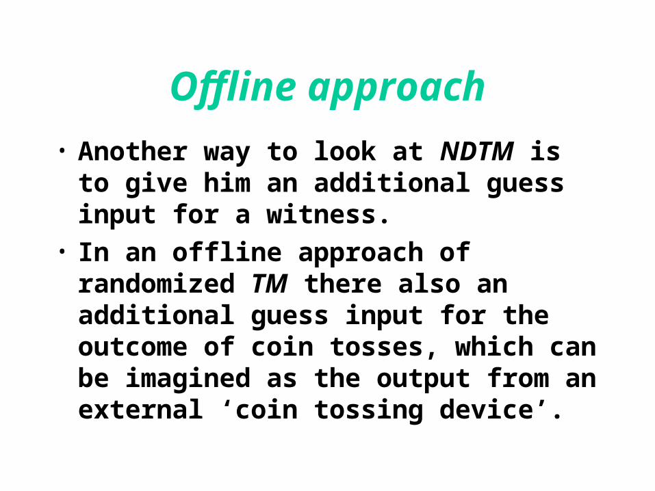
Offline approach

• Another way to look at NDTM is to give him an additional guess input for a witness.

• In an offline approach of randomized TM there also an additional guess input for the outcome of coin tosses, which can be imagined as the output from an external ‘coin tossing device’.

Offline approach (cont)

• A language LNP iff there exists a DTM M and a polynomial p(), s.t. for every xL y |y|p(|x|) and M(x,y) accepts.

• The DTM has access to a “witness” string of polynomial length.

• Similarly, a random TM has access to a “guess” input string. But there must be sufficient such witnesses

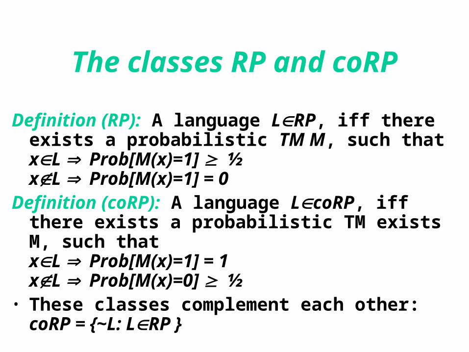
Definition (RP): A language LRP, iff there exists a probabilistic TM M, such that xL Prob[M(x)=1] ½ xL Prob[M(x)=1] = 0

Definition (coRP): A language LcoRP, iff there exists a probabilistic TM exists M, such thatxL Prob[M(x)=1] = 1xL Prob[M(x)=0] ½

• These classes complement each other:coRP = {~L: LRP }

The classes RP and coRP

Comparing RP with NP

Let L be a language in NP or in RP. Let RL be the relation defining the witness/guess

for L for a certain TM. Then the definition for NP and RP are:

L NP L RP

xL y s.t. (x,y)RL xL Prob[(x,r)RL] ½

xL y (x,y)RL xL r (x,r)RL

Explanations

Claim: RPNP

• Let L be an arbitrary language in RP. If x L then there exist a TM M and a coin-tosses y such that M(x,y)=1 in more than ½ coin tosses. We can use the same coin toss y as a witness. If x L then Probr[M(x,r) = 1] = 0, so there is no witness. ∎

Explanations

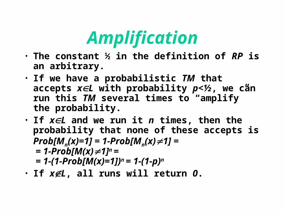
Amplification• The constant ½ in the definition of RP is an

arbitrary.• If we have a probabilistic TM that accepts xL

with probability p<½, we can run this TM several times to “amplify” the probability.

• If xL and we run it n times, then the probability that none of these accepts isProb[Mn(x)=1] = 1-Prob[Mn(x)1] = = 1-Prob[M(x)1]n = = 1-(1-Prob[M(x)=1])n = 1-(1-p)n

• If xL, all runs will return 0.

Explanations

Alternative Definitions for RP (RP1 and RP2)

Definition (RP1): LRP1 iff probabilistic Poly-time TM M and a polynomial p(), s.t. xL Prob[M(x)=1] xL Prob[M(x)=1] = 0

Definition (RP2): LRP2 iff probabilistic Poly-time TM M and a polynomial p(), s.t. xL Prob[M(x)=1] 1-2-p(|x|)

xL Prob[M(x)=1] = 0

)(1 xp

Explanations• The definitions for RP1 and RP2 seem to be very

far from each other, because:– RP1 answers correctly with a very small probability

(but not negligible)– RP2 can almost ignore the probability of it’s

mistake.

• However these two definitions actually define the same class.

• This implies that having algorithm with a noticeable probability of success implies existence of an efficient algorithm with negligible probability of error.

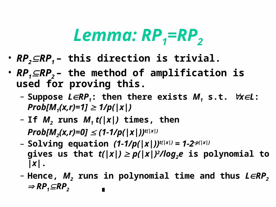
Lemma: RP1=RP2

• RP2RP1 – this direction is trivial. • RP1RP2 – the method of amplification is used for

proving this.– Suppose LRP1: then there exists M1 s.t. xL:

Prob[M1(x,r)=1] 1/p(|x|)– If M2 runs M1 t(|x|) times, then

Prob[M2(x,r)=0] (1-1/p(|x|))t(|x|)

– Solving equation (1-1/p(|x|))t(|x|) = 1-2-p(|x|) gives us that t(|x|) p(|x|)2/log2e is polynomial to |x|.

– Hence, M2 runs in polynomial time and thus LRP2 RP1RP2 ∎

Explanations• RP2RP1: if |x||x| is long enough, then

1-2-p(|x|) 1/p(|x|). So being in RP2 implies being in RP1 for almost all inputs.

• Claim: RPRP1 = RP2

– RP2RP : if |x||x| is long enough, then 1-2-p(|x|) ½.

– RPRP1 : if |x||x| is long enough, then ½ 1/p(|x|).

– From these two claims, it follows that : RP2RP RP1 .

– It was proven beforehand that RP1 = RP2 and with

RP2RP RP1 , we get that RPRP1 = RP2 . ∎

The class BPP

Definition (BPP): LBPP iff there exists a polynomial-time probabilistic TM M, such that

xL: Prob[M(x)=L(x)] 32

Explanations• We can say that RP is too strict because it ask that the machine

has to give 100% correct answer for inputs that are not in the language.

• We derived the definition of RP from the definition of NP , but NP didn't reflect an actual computational model for search problems but rather a model for verification.

• But it seems that looking at a two sided error is more appealing as a model for search problem computations.

• We want a machine that will recognize the language with high probability, where probability refers to the event “The machine answers correctly on an input x regardless if x L or x L”.

Explanations• The BPP machine is a machine that makes mistakes

but returns the correct answer most of the time.• By running the machine a large number of times and

returning the majority of the answers we are guaranteed by the law of large numbers that our mistake will be very small.

• The idea behind the BPP class is that M accept by majority with a noticeable gap between the probability to accept inputs that are in language and the probability to accept inputs that are not in the language, and it's running time is bounded by a polynomial.

Invariance of constant

• The in the definition of BPP is, again, an arbitrary constant. Replacing the

in the definition by any other constant greater than ½ does not change the class defined.

32

32

Explanations• In the RP case we had two probability spaces that we

could distinguish easily because we had a guarantee that if x L then the probability to get one is zero, hence if you get M(x) = 1 for some input x, you could say for sure that x L.

• In the BPP case, the amplification is less trivial because we have zeroes and ones in both probability spaces.

• The reason that we can apply amplification in the BPP case is that invoking the machine many times and counting how many times it returns one gives us an estimation on the fraction of ones in the whole probability space.

Invariance of constant(cont)

• We consider the following change of constants:xL Prob[M(x)=1] p+xL Prob[M(x)=1] p-for any given p (0,1) and 0 < < min{p,1-p}.

• We can build a machine M2 that runs M n times, and return the majority of results of M. After a constant number of executions (depending on p and but not on x) we would get the desired probability.

Explanations

The weakest possible BPP definition(BPP1)

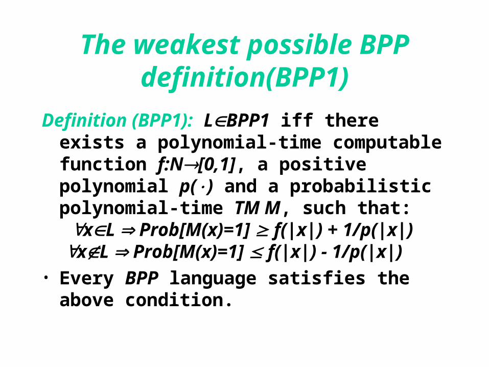
Definition (BPP1): LBPP1 iff there exists a polynomial-time computable function f:N[0,1], a positive polynomial p() and a probabilistic polynomial-time TM M, such that:

xL Prob[M(x)=1] f(|x|) + 1/p(|x|) xL Prob[M(x)=1] f(|x|) - 1/p(|x|)

• Every BPP language satisfies the above condition.

Explanations

If we set f(|x|)=½ and p(|x|)=6 we get the original definition.

Original definition of BPP is:

LBPP iff there exists a polynomial-time probabilistic TM M, such that

xL: Prob[M(x)=L(x)] 32

Claim: BPP=BPP1

Proof:• Let LBPP1 and let M be its computing TM.• Then, for any given input x, we look at the random variable

M(x), which is a Bernoulli random variable with unknown parameter p = Exp[M(x)].

• Using a well known fact that the expectation of a Bernoulli random variable is exactly the probability to get one we get that p = Prob[M(x) = 1].

• So by estimating p we can say something about whether x L or x L.

• The most natural estimator is to take the mean of n samples of the random variable.

ExplanationsBernoulli random variable • A Bernoulli trial is an experiment that can result in

only one of two possible outcomes, labeled success and failure. 

• The Bernoulli random variable is defined as X=0 if a failure occurs and X=1 if a success occurs.

• If p = P(success) then E(X) = p and Var(X) = p(1-p).• In our case we use a fact that the expectation of a

Bernoulli random variable is exactly the probability to get one(success).

Explanations• We will use the known statistical method of confidence

intervals on the parameter p. • The confidence interval method gives a bound within

which a parameter is expected to lie with a certain probability.

• Interval estimation of a parameter is often useful in observing the accuracy of an estimator as well as in making statistical inferences about the parameter in question.

Claim: BPP=BPP1(cont)

• In our case we want to know with probability higher than if p [0, f(|x|) - 1/p(|x|)]

or p [f(|x|) + 1/p(|x|), 1].• This is enough because if p [0, f(|x|) - 1/p(|x|)]

then x L and if p [f(|x|) + 1/p(|x|), 1] then

x L.• Note that p (f(|x|) - 1/p(|x|),f(|x|) + 1/p(|x|)) is

impossible.

32

Explanations• Because we assumed that LBPP1 then

according to BPP1 definition :

xL Prob[M(x)=1] f(|x|) + 1/p(|x|)xL Prob[M(x)=1] f(|x|) - 1/p(|x|)

• We get that :

p (f(|x|) - 1/p(|x|),f(|x|) + 1/p(|x|)) is impossible.

Claim: BPP=BPP1(cont)

• Define M’(x) invoke ti=M(x) i=1…n, compute p=ti/n, if p>f(|x|) return YES else return NO.

• Notice p is exactly the mean of a sample of size n taken from the random variable M(x).

Explanations• This machine does the normal statistical process of

estimating a random variable by taking samples and using the mean as an estimator for the expectation.

• If we will be able to show that with an appropriate n the estimator will not fall too far from the real value with a good probability, it will follow that this machine answers correctly with the same probability.

• To resolve n we will use Chernoff's inequality.

Claim: BPP=BPP1(cont)

2δ2n

n

4

12

2δ

np1p2

2δn

1i i e2e2e2δpnΧ

Prob

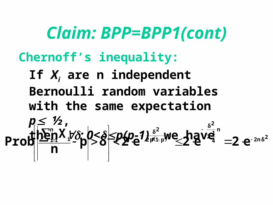
Chernoff’s inequality:

If Xi are n independent Bernoulli random variables with the same expectation p½,then : 0<p(p-1), we have

Claim: BPP=BPP1(cont)

• By setting and

we get that our Turing machine M’ will decide L(M) with probability greater than , suggesting that L(M) BPP. ∎

)xp(

1δ

2δ261ln

n

32

The strongest possible BPP definition(BPP2)

Definition (BPP2): LBPP2 iff there exists a polynomial-time probabilistic TM M and a polynomial p(), such that xL Prob[M(x)=L(x)] 1-2-p(|x|).

Explanations

• If we set p(|x|)=2 we get the original definition, because 1-2-2

• Hence, BPP2BPP.

32

Claim: BPP=BPP2

• Let LBPP and let M be its computing TM.• We can amplify the probability of right answer

by invoking M many times and taking the majority of it's answers.

• Define: M’(x) invoke ti=M(x) i=1…n,

compute p=ti/n,

if p > ½ return YES

else return NO.

Claim: BPP=BPP2(cont)

• From the original definition, we get that if we know that Exp[M(x)] > ½ it follows that x L and if we know that Exp[M(x)] < ½ it follows that x L.

• But original definition gives us more. It says that the expectation of M(x) is bounded away from ½ so we can use the confidence interval method.

Explanations

Original definition of BPP is:

LBPP iff there exists a polynomial-time probabilistic TM M, such that

xL: Prob[M(x)=L(x)]

• The confidence interval method gives a bound within which a parameter is expected to lie with a certain probability.

32

Claim: BPP=BPP2(cont)

• From Chernoff’s inequality we get that:

Prob[|M’(x)-Exp[M(x)]|2e-n/18

• But if |M’(x)-Exp[M(x)]| < we get that the answer of M’ is correct, because it is close enough to the the expectation of M(x) which is guaranteed to be above when x L and below when x L.

32

31

61

61

Claim: BPP=BPP2(cont)

• So we get that:

Prob[M’(x)=L(x)] 1-2e-n/18.

• If we choose n=18ln(2)p(|x|) we get the desired probability. ∎

Explanations• We see that a gap of 1/p(|x|) and a gap of

1- 2-p(|x|) which look like “weak” and “strong” versions of BPP are the same.

• As shown above the “weak” version is actually equivalent to the “strong” version, and both are equivalent to the original definition of BPP.

Some comments about BPP• RPBPP – one side error is a special

case of two sided error.• It’s not known if BPPNP. It might be

so but we don't get it from the definition like we did in RP.

• coBPP = BPP from the symmetry of the definition of BPP.

• And of course P BPP.

The class PP

Definition (PP): LPP iff exists a polynomial-time probabilistic TM M s.t.

xL Prob[M(x)=1] > ½ xL Prob[M(x)=1] < ½

Explanations• The class PP is wider than what we have seen so far. • In the BPP case we had a gap between the number of

accepting computations and non accepting computations. This gap enabled us to determine with good probability if x L or x L.

• The gap was wide enough so we could invoke the machine polynomially many times and notice the difference between inputs that are in the language and inputs that are not in the language.

• The PP class don't put the gap restriction, hence the gap may be very small (even one guess can make a difference), so running the machine polynomially many times may not help.

Claim: PP PSPACE

• Let LPP, M be the TM that recognizes Land p(|x|) be the time bound.

• Define M’(x) run M(x) using all p(|x|) possible coin tosses and decide by majority.

• M’ uses polynomial space for each of the invocations and answers correctly since M is a PP machine that answers correctly for more than half of the guesses.

The class PP1

Definition (PP1):L PP1 iff exists a polynomial-time

probabilistic TM M s.t.

xL Prob[M(x)=1] > ½ xL Prob[M(x)=1] £ ½

Note: PP PP1.

Explanations

The idea of class PP1: since we cannot add the equal

value to both xL and xL cases (because it will not

give us information – any coin flipping will satisfy the

definition), we want to try it in xL case only ,

and to show that it will not change the class of languages.

Obviously , PP PP1 since if exists a machine that

satisfies PP definition , it clearly satisfies PP1 definition.

Claim: PP1 PP

Proof :Let LPP1, M be the TM that recognizes Land p(|x|) be the time bound.

• M’(x,(a1,a2,...,ap(|x|),b1,b2,...,bp(|x|))) if ( a1=a2=...=ap(|x|)=1 )

return NO else

return M(x,(b1,b2,...,bp(|x|)))

Explanations

• We define MM’ that choose one of two possible moves. One move, which happens with probability 2-p(|x|)+1 , will return NO.The second move , which happens with probability 1-2-p(|x|)+1 , will invoke M with independent coin tosses.

• Note: M' is exactly the same as M, except for an additional probability of 2-p(|x|)+1 for returning NO.

Claim: PP1 PP (cont)

• xL Prob[M(x)=1] > ½ Prob[M(x)=1] ³ ½+2-p(|x|)+1 Prob[M’(x)=1] ³ (½+2-p(|x|))(1-2-p(|x|)+1) > ½

• xL Prob[M(x)=0] ³ ½ Prob[M’(x)=1] ³ ½(1-2-p(|x|)+1)+2-p(|x|)+1 > ½

Thus PP1 PP PP1 = PP ∎

Claim: NPPP

• Let LNP, M be the NDTM that recognizes L, and p(|x|) be the time bound.

• M’(x,(b1,b2,...,bp(|x|)))

if ( b1=1 )

return M(x,(b2,...,bp(|x|)))

else

return YES

Explanations

• We define MM’ that uses it's random coin-tosses as a witness to M with only one toss that it does not pass to M’.

This toss is used to choose it's move. One of the two possible moves gets it to the ordinary computation of M with the same input (and the witness is the random input). The other choice gets it to the computation that always accepts.

Claim: NPPP (cont)

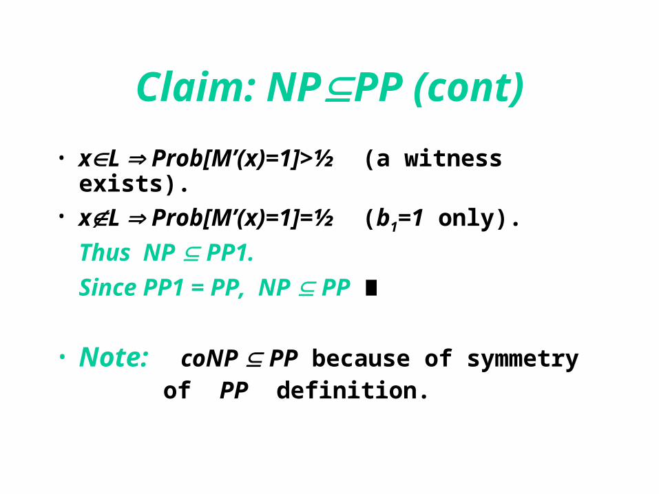
• xL Prob[M’(x)=1]>½ (a witness exists).• xL Prob[M’(x)=1]=½ (b1=1 only).

Thus NP PP1.

Since PP1 = PP, NP PP ∎

• Note: coNP PP because of symmetry of PP definition.

The class ZPP

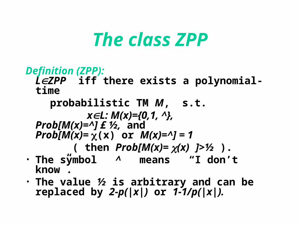
Definition (ZPP):LZPP iff there exists a polynomial-time

probabilistic TM M, s.t. xL: M(x)={0,1, ^},

Prob[M(x)=^] £ ½, and Prob[M(x)= (x) or M(x)=^] = 1

( then Prob[M(x)= (x) ]>½ ).• The symbol ^ means “I don’t know”.• The value ½ is arbitrary and can be replaced

by 2-p(|x|) or 1-1/p(|x|).

Explanations

The idea of class ZPP: we want to let the machine say

“I don’t know” for some inputs. We define the machine

that will never give a wrong answer - it will say “I don’t

know” if it is not sure. Same time , this machine

will define class , that will be equal (as we will prove)

to RPcoRP.

Claim: ZPP = RP coRP

• Let LZPP, M be a polynomial-time probabilistic TM recognizes L.

• let b=M(x).• M’(x)

if ( b = ^ ) return 0else return b

Claim: ZPP = RP coRP (cont)

• xL Prob[M’(x)=1]>½.• xL M’(x) will never return 1.

Thus ZPP RP.

Note: The proof that ZPP is in coRP

is similar ∎

Explanations

• We define MM’ so that for xL the probability of getting the right answer with M’ is greater than ½ and M’s definite answer are always correct (it never return a wrong answer because it returns ^ when it is uncertain).

In case that xL , by returning 0

when M(x) = ^ we will always answer

correctly , because in this case

M(x)!=^ M’(x)= (x) M’(x)=

Randomized space complexity

Definition (RSPACE):

LRSPACE(S) iff

there exists a randomized TM M s.t.

x {0,1}*xL Prob[M(x)=1] ½ xL Prob[M(x)=1] = 0and M uses at most S(|x|) space and

runs at most exp(S(|x|)) time.

Randomized space complexity

Definition (badRSPACE):

LbadRSPACE(S) iff

there exists a randomized TM M s.t.

x {0, 1}*xL Prob[M(x)=1] ½ xL Prob[M(x)=1] = 0and M uses at most S(|x|) space

Explanations

• Note: RSPACE machine has both

space and time restriction ,

while badRSPACE has no time restriction.

Claim: badRSPACE(S)=NSPACE(S)

• Let LbadRSPACE(S).• xL x NSPACE(S).• xL x NSPACE(S).

• Thus badRSPACE(S) NSPACE(S)

Explanations

• If xL , there are many witnesses

( but one is enough). Thus x NSPACE(S).

On other hand , if xL , there are no

witness , thus x NSPACE(S).

Claim: badRSPACE(S)=NSPACE(S)

(cont)

• Let LNSPACE(S), and M be the NDTM for L, which decides L in space S(|x|).

• For every x L, there an accepting computation in exp(S(|x|)) time

r , |r| < exp(S(|x|)) s.t. M(x,r)=1.• Thus , for uniform distributed random r:

Prob[M(x,r)=1] ³ exp(S(|x|)) .

Claim: badRSPACE(S)=NSPACE(S)

(cont)

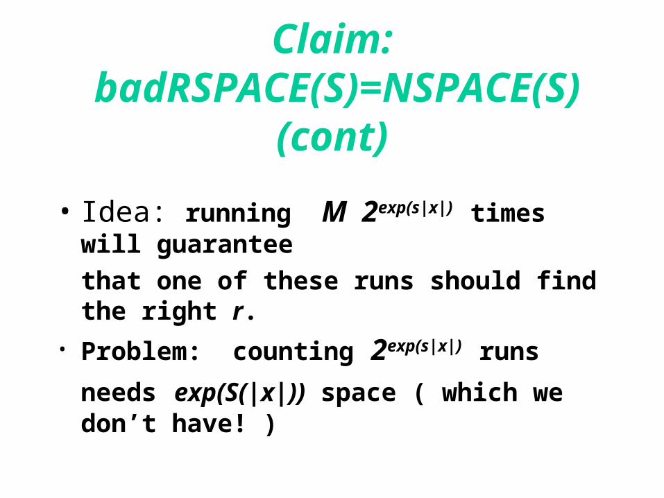
• Idea: running M 2exp(s|x|) times will guarantee

that one of these runs should find the right r.

• Problem: counting 2exp(s|x|) runs

needs exp(S(|x|)) space ( which we don’t have! )

Claim: badRSPACE(S)=NSPACE(S)

(cont)

• Solution: A randomized counter of

k = log2 2exp(s|x|) = exp(S(|x|)) coins which stops

the algorithm when i ki=1.

As a result , we don’t have to store k tosses,

we only have to count to k, which takes

log(k) = log(exp(S(|x|))) = s(|x|) space.

Thus LbadRSPACE(S) .∎

Explanations

• Some general facts:

• P ZPP RP BPP

• P ZPP coRPBPP