RANDOM WALKS FROM STATISTICALPHYSICS I

Random Walks: Simple and Self-AvoidingWald Lectures

2011 Joint Statistical Meetings

Gregory F. Lawler

Department of MathematicsDepartment of Statistics

University of Chicago

August 2, 2011

1 / 24

I Random walks appear in many places in statistical physics.

I Behavior strongly depends on the dimension in which the walklives. Our walks will live in the integer lattice

Zd = {(z1, . . . , zd) : zj ∈ Z}.

The choice of lattice is not so important (universality) but thedimension d is.

I There is an upper critical dimension above which the behavioris in some sense easy to understand (mean-field behavior)

I Below the critical dimension, there are nontrivial “criticalexponents”

I Still many open questions in these areas.

I Today I will introduce some models and will discuss alldimensions. The second two lectures will focus on work in thelast twelve years on two-dimensional systems where conformalinvariance becomes important.

2 / 24

SIMPLE RANDOM WALK

I At each step the random walker chooses randomly among its2d nearest neighbors to move to.

I Can write the position of the walker at time n as

Sn = X1 + · · ·+ Xn

where X1, . . . ,Xn are independent, identically distributed,mean zero.

I Classical probability — E[|Sn|2] = n and Sn/√

n converges indistribution to a standard normal random variable.

I At time n the walker is distance of order√

n away from theorigin. Assuming d ≥ 2, we can restate this as “the numberof points in the ball of radius R visited by the walker is R2.

I The “fractal dimension” of the set of points visited by thewalker is 2. This holds for all d ≥ 2.

3 / 24

FRACTAL DIMENSION

I Roughly speaking, a subset of Zd has fractal dimension D ifthe number of points in the disk of radius R grows like RD .Note that D ≤ d .

I The rule for variance of sums of independent random walksshows that the fractal dimension of simple random walk pathis D = 2 (provided that d ≥ 2).

I There are a number of rigorous notions of fractal dimensionsuch as Hausdorff dimension and box dimension. We will notgo into details about this.

I The Hausdorff or box dimension of the path of Brownianmotion in Rd is two.

4 / 24

WARM-UP: USING “DIMENSIONAL” ARGUMENTS

I What is the probability that a random walk is at the origin attime 2n?

I The walk is about distance√

n from the origin.

I There are about nd/2 points in Zd at that distance.

I The probability of being at a particular one is n−d/2. Thisindicates the result

P{S(2n) = 0} ∼ c n−d/2.

I Let en denote the expected number of visits up to time n.Then e∞ < ∞ for d ≥ 3 and

en ∼ c n1/2, , d = 1

en ∼ c (log n) d = 2.

5 / 24

I Two is the critical dimension. This is the critical dimensionfor intersection of a two-dimensional set (random walk) and azero-dimensional set (origin).

I Let pn denote the probability that the walk does not return upto time n. It can be shown that

pn ³ 1

en³

n−1/2, d = 1(log n)−1, d = 21, d ≥ 3

I This argument uses a Markov or renewal argument — if arandom walk returns to the origin, then the expected numberof visits after that is the same as the expected number (Thislast argument is easier if we allow a geometric number ofsteps which is the same as generating function techniques.)

I In particular, we get Polya’s theorem that the random walk isrecurrent if and only if d ≤ 2.

6 / 24

SELF-AVOIDING WALK (SAW)

I A self-avoiding walk (SAW) of length n is a simple randomwalk path that does not visit any vertex more than once.

I Used as a model of polymer chains. (A polymer consists ofmonomers that form themselves randomly with the constraintthat it cannot come back on itself.)

I Analyzing SAWs is much harder than simple random walks.Many questions remain open today.

I Let cn denote the number of SAWs of length n starting at theorigin. (The number of simple walks is (2d)n.) There is aconnective constant µ such that

cn ≈ µn.

I Numerically we know that µ ≈ 2.64 if d = 2. There is a goodchance we will never know the number exactly.

I The number µ depends on the lattice. Duminil-Copin andSmirnov recently proved a conjecture by Nienhuis that on the

honeycomb lattice µ =√

2 +√

2.

7 / 24

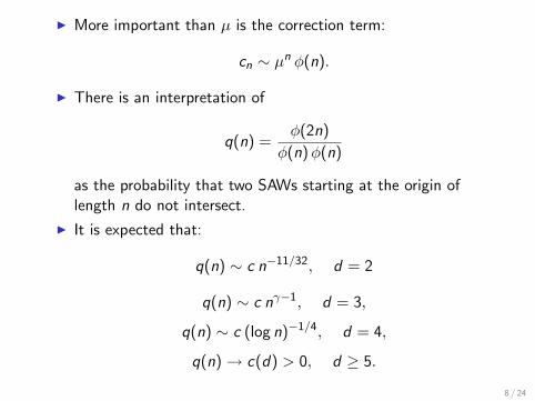
I More important than µ is the correction term:

cn ∼ µn φ(n).

I There is an interpretation of

q(n) =φ(2n)

φ(n) φ(n)

as the probability that two SAWs starting at the origin oflength n do not intersect.

I It is expected that:

q(n) ∼ c n−11/32, d = 2

q(n) ∼ c nγ−1, d = 3,

q(n) ∼ c (log n)−1/4, d = 4,

q(n) → c(d) > 0, d ≥ 5.

8 / 24

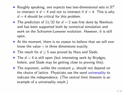
I Roughly speaking, one expects two two-dimensional sets in Rd

to intersect it d < 4 and not to intersect if d > 4. This is whyd = 4 should be critical for this problem.

I The prediction of 11/32 for d = 2 was first done by Nienhuisand has been supported both by numerical simulation andwork on the Schramm-Loewner evolution. However, it is stillopen.

I At the moment, there is no reason to believe that we will everknow the value γ in three dimensions exactly.

I The result for d ≥ 5 was proved by Hara and Slade.

I The d = 4 is still open (but interesting work by Brydges,Imbrie, and Slade may be getting close to proving this).

I The exponent, unlike the constant µ, should not depend onthe choice of lattice. Physicists use the word universality toindicate the independence. (The central limit theorem is anexample of a universality result.)

9 / 24

I Another critical exponent for the SAW ν = νd is defined bysaying that the typical displacement of a SAW of n steps lookslike nν .

I For simple random walks ν = 1/2 for all d .

I Flory gave a heuristic argument to suggest that

νd = max

{1

2,

3

d + 2

}.

I Trivial if d = 1. Not at all trivial but proved by Hara andSlade if d ≥ 5.

I For d = 4 a logarithmic correction is expected. Not proved.

I For d = 2 it is expected to be true. Although it has not beenproved, the exponent can be seen in the fractal dimension ofthe conjectured scaling limit (Schramm-Loewner evolution)

I For d = 3, the prediction is not expected to be exactly true.Numerically ν3 ≈ .58 · · · . Perhaps this number will never beknown exactly.

10 / 24

ANALOGOUS QUESTION:INTERSECTIONS OF RANDOM WALK PATHS

I Let S1 and S2 be independent simple random walks in Zd

starting at the origin. Let

ωn = {S1(j) : j = 1, . . . , n}, ηn = {S2(j) : j = 1, . . . , n},

q(n) = P{ωn ∩ ηn = ∅}.I This is analogous (but not the same!) as the quantity for

SAW.

I The expected number of intersections tends to infinity if andonly if d ≤ 4.

I If d ≥ 5, q(n) → q(∞) > 0.

I For d = 1, one can show that q(n) ³ n−1. (The blue and redstay in different half lines. The gambler’s ruin estimate forsimple random walk is the key tool.)

11 / 24

EASIER PROBLEM

λn = {S3(j) : j = 1, . . . , n}.p(n) = P{ωn ∩ [ηn ∪ λn] = ∅}.

I The origin looks like a “middle point” of the random walkpath ηn ∪ λn. This makes the quantity easier to estimate.

I Determining p(n) is not so difficult

p(n) ³ n−α, α = αd =4− d

2d < 4,

p(n) ³ (log n)−1, d = 4.

I p(n) equals

P{ωn ∩ ηn = ∅}P{ωn ∩ λn = ∅ | ωn ∩ ηn = ∅}.I Cauchy-Schwarz implies q(n)2 ≤ p(n) ≤ q(n).

12 / 24

I Mean-field behavior would be

P{ωn ∩ λn = ∅ | ωn ∩ ηn = ∅} ³ P{ωn ∩ λn = ∅}.I If mean-field, then p(n) ³ q(n)2.

I Systems at the critical dimension tend to exhibit mean-fieldbehavior. This is true here [L]: if d = 4,

q(n) ³ p(n)1/2 ³ (log n)−1/2.

I If d = 1, q(n) ³ n−1, p(n) ³ n−3/2. Not mean-field.

I If d = 2, 3, it is not mean-field. In fact [Burdzy-L], thereexists an intersection exponent ζ = ζd such that

q(n) ³ n−ζ .

This is the same as an exponent for Brownian motion.

I The argument shows existence of the exponent, but does notcompute its value.

13 / 24

I Estimates were given for the exponent ζ. In particular,

4− d

4< ζd <

4− d

2.

I Duplantier and Kwon gave a nonrigorous, physical argumentusing conformal field theory to predict ζ2 = 5/8. This wasconsistent with simulations.

I This prediction was proved by L-Schramm-Werner using theSchramm Loewner evolution (SLE).

I Numerical simulations suggest .28 < ζ3 < .29. It is possiblethat this value will never be known exactly!

I Relates to fractal nature of Brownian motion paths. SupposeBt , 0 ≤ t ≤ 1 is a d-dimensional Brownian motion (d = 2, 3).A cut time is a time that satisfies

B[0, t) ∩ B(t, 1] = ∅.Then (w.p.1), almost all times t will not be cut times. In fact,the Hausdorff dimension of the set of cut times is 1− ζd .

14 / 24

A PROBLEM OF MANDELBROT

I In his Fractal Geometry of Nature, Benoit Mandelbrot lookedat Brownian islands obtained by taking a planar Brownianmotion or random loop and filling in the bounded areas. Thecoastline is also called the ”Brownian frontier”.

I The frontier looked to him to have the same fractalcharacteristics as self-avoiding walk. In particular, the fractaldimension was 4/3.

I Studying this leads to the disconnection exponent λ definedby saying that the probability that a two-sided n-step randomwalk does not disconnect the origin decays like n−λ. (Such apoint looks like a typical point of the frontier.)

I Similar methods show that this exists and is equivalent to aBrownian exponent. The Hausdorff dimension of theboundary is 2(1− λ). This method did not compute λ.

15 / 24

I The nonrigorous prediction λ = 1/3 was made usingconformal field theory.

I The disconnection exponent is a type of intersection exponentand LSW proved Mandelbrot’s conjecture by showing λ = 1/3.

I Further work has shown that Mandelbrot was even “moreright”. The statistics of the outer boundary of the Brownianmotion are very similar to the conjectured scaling limit ofself-avoiding walk.

I In three dimensions, the outer boundary is the same as theentire path. However, one can consider the “dimension ofharmonic measure” which is the effective dimension of the setwhich are the first visit of a Brownian motion. One can provethat this dimension is strictly less than two (multifractalbehavior).

I In contrast, the effective dimension in two dimensions is one.(This is true for all connected sets by a theorem of Makarov.)

16 / 24

LOOP-ERASED RANDOM WALK

I Take a simple random walk path and erase loopschronologically.

I Easy to define for d ≥ 3 (random walk is transient). Need alimiting argument (not too difficult) for d = 2. (d = 1 is notinteresting)

I First considered in order to hope to understand self-avoidingwalk. However, it turns out that the paths look qualitativelydifferent. (Physicists would say that it is in a differentuniversality class.)

I The problem turns out to be related to a number of otherproblems: electrical networks, uniform spanning trees,determinant of the Laplacian. We will not consider thesetoday.

I We ask: how far does a loop-erased walk go in n steps?

17 / 24

I Let Yn be the number of steps on an n step walk that remainafter loop erasure. Define Φ(n) by

Φ(n) = E[Yn]

In Φ(n) steps one expects to be distance n1/2.

I In n steps expect distance [Φ−1(n)]1/2.

I Critical dimension is d = 4.

I If d > 4, with probability one Yn ∼ c n and the loop-erasedrandom walk has the scaling limit as random walk (Brownianmotion).

18 / 24

I Let Jn be the conditional probability given [S(0), . . . , S(n)] ofthe event that the nth point of the simple random walk is noterased. The probability that the nth point is not erased isE[Jn].

I The “easy” quantity to compute turns out to be the thirdmoment (recall: returns to origin — first moment;intersections of random walks — second moment)

E[J3n

] ³{

n(d−4)/2 d = 2, 3(log n)−1 d = 4.

I “Mean-field” corresponds to E[J3n

] ≈ E[Jn]3. Expect to be

true if d = 4 but not if d = 2, 3.

I If d = 4, E[Jn] ³ (log n)−1/3 and the typical path hasn/(log n)1/3 points. The typical distance of an n-step walk isn1/2 (log n)1/6. Moreover the scaled process approaches aBrownian motion.

19 / 24

I For d = 2, 3 define α = αd by E[Jn] ³ n−α. In other wordsthe loop-erasure of an n-step path has n1−α points.

I Let ν = νd denote the exponent given by the typical distancein n steps is nν .Since [n1−α]ν ≈ n1/2,

ν =1

2(1− α).

I Since E[J3n ] ≈ n(d−4)/2, we see that α ≥ (4− d)/6. This

gives the inequality

ν ≥ 3

2 + d.

The right-hand side is the Flory guess for the exponent forSAW. Since we expect not mean-field behavior, would guessthat equality does not hold.

I This indicates that loop-erased walks are “thinner” thanself-avoiding walks. (There are other heuristic arguments forthis.)

20 / 24

I For d = 2, Kenyon used an analogy with dimers and acalculation using conformal invariance to show that

ν2 = 4/5.

I LSW showed later that the scaling limit of loop-erased walkfor d = 2 is SLE with κ = 2. This is the value such that thepaths have fractal dimension 5/4.

I For d = 3 the exponent is not known exactly and it is notknown if it ever will. Wilson did numerics recently suggestingν3 = .6157 · · · .

21 / 24

LAPLACIAN RANDOM WALK

I The loop-erased random walk (LERW) is equivalent to amodel called the Laplacian random walk

I We will give the definition in the transient (d ≥ 3) case.There is a similar definition for d = 2.

I Let S0, S1, . . . denote the loop-erased walk and letωn = [S0, . . . , Sn].

I The LERW is a non-Markovian process, but we can still givetransition probabilities

I Let p(z) be the probability that a simple random walk startingat z never visits ωn. By definition p(z) = 0 if z ∈ ωn. Then,

P{Sn+1 = z | ωn} ∝ p(z).

22 / 24

I p(z) is the unique discrete harmonic function (satisfyingdiscrete Laplace equation) with boundary value 0 on ωn and 1at infinity.

I If d = 2, the boundary condition at infinity becomesp(z) ∼ log |z |.

I At least heuristically, we can write a similar expression forself-avoiding walks, except that p(z) is replaced with theprobability that a self-avoiding walk avoids ωn. Since it shouldbe easier for a SAW to avoid the set, we would guess that theSAW paths are not pushed to infinity as quickly. This is whythey should be thicker than LERW paths.

I One can create a one-parameter family of processes by sayingthat

P{Sn+1 = z | ωn} ∝ p(z)b.

This is most interesting in two and three dimensions wherethe fractal dimension is expected to vary with b.

I For d = 2, there is a one parameter family of continuousprocess, SLE.

23 / 24

SUMMARY

We have looked at three problems: SAW, intersection of randomwalks, loop-erased walk. There are many other models in “criticalphenomenon” with these properties:

I An (upper) critical dimension above which behavior is trivial.

I Mean-field behavior at the critical value with logarithmiccorrection.

I Non mean-field behavior below the critical value withnontrivial “critical exponents”

I In dimensions strictly between 2 and the critical dimension, itmay not be possible to give value exactly.

I In two dimensions, conformal invariance plays a major role.Here critical exponents can be determined exactly.

I Much progress has been made in the last twelve years in thetwo dimensional case. The second two lectures in this serieswill discuss this.

24 / 24