Random Intercept and Slope Models - Edps/Psych/Stat...
189
Random Intercept and Slope Models Edps/Psych/Stat 587 Carolyn J. Anderson Department of Educational Psychology ILLINOIS university of illinois at urbana-champaign c Board of Trustees, University of Illinois Fall 2013
-
Upload
nguyenmien -
Category
Documents
-
view
228 -
download
0
Transcript of Random Intercept and Slope Models - Edps/Psych/Stat...

Random Intercept and Slope ModelsEdps/Psych/Stat 587
Carolyn J. Anderson
Department of Educational Psychology
I L L I N O I Suniversity of illinois at urbana-champaign
c© Board of Trustees, University of Illinois
Fall 2013

Overview Intercepts & Slopes Multiple Micro Categorical Predictors NELS Cross-Level Centering Summary SAS
Outline
◮ Random intercepts and slopes with one mirco-variable.
◮ Multiple Micro-level variables.
◮ Discrete Random Effects.
◮ NELS Example.
◮ Cross-level interactions (macro level variables).
◮ Centering Level 1 Variables.
◮ SAS/MIXED.
◮ Computer Lab Session 2.
Snijders & Bosker (2012) Chapter 5
C.J. Anderson (Illinois) Random Intercept and Slope Models Fall 2013 2.1/ 189

Overview Intercepts & Slopes Multiple Micro Categorical Predictors NELS Cross-Level Centering Summary SAS
A Little Motivation
From the HSB data that we looked at before. . .
C.J. Anderson (Illinois) Random Intercept and Slope Models Fall 2013 3.1/ 189

Overview Intercepts & Slopes Multiple Micro Categorical Predictors NELS Cross-Level Centering Summary SAS
Random Intercepts & Slopes (1 xij)The model and it’s properties:
Level 1:Yij = β0j + β1jxij + Rij
where Rij ∼ N (0, σ2).
Level 2:
β0j = γ00 + U0j
β1j = γ10 + U1j
where (U0j
U1j
)= Uj ∼ N
((00
),
(τ20 τ10τ10 τ21
))
and independent over j and with Rij .C.J. Anderson (Illinois) Random Intercept and Slope Models Fall 2013 4.1/ 189
Overview Intercepts & Slopes Multiple Micro Categorical Predictors NELS Cross-Level Centering Summary SAS
Level 2 Models
Notes:
◮ τ20 is the variance of the level 2 residuals U0j from predictingthe level 1 intercept (i.e, β0j ).
◮ τ21 is the variance of the level 2 residualsU1j from predictingthe level 1 slope (i.e, β1j ).
◮ τ10 is the covariance between U0j and U1j .
cov(U0j ,U1j) = cov(β0j , β1j ) = τ10.
How to interpret τ10?
C.J. Anderson (Illinois) Random Intercept and Slope Models Fall 2013 5.1/ 189

Overview Intercepts & Slopes Multiple Micro Categorical Predictors NELS Cross-Level Centering Summary SAS
Interpreting τ10Suppose that the following two schools from the 1003 NELS88 aretypical of what’s in the population.
Would you expect τ10 <,=,or > 0?
C.J. Anderson (Illinois) Random Intercept and Slope Models Fall 2013 6.1/ 189

Overview Intercepts & Slopes Multiple Micro Categorical Predictors NELS Cross-Level Centering Summary SAS
The Linear Mixed Model
Yij = (γ00 + U0j) + (γ10 + U1j)xij + Rij
= γ00 + γ10xij︸ ︷︷ ︸+U0j + U1jxij + Rij︸ ︷︷ ︸fixed random
What’s the variance of Yij?
C.J. Anderson (Illinois) Random Intercept and Slope Models Fall 2013 7.1/ 189

Overview Intercepts & Slopes Multiple Micro Categorical Predictors NELS Cross-Level Centering Summary SAS
The Variance of Yij
var(Yij) ≡ E[(Yij − E(Yij))2]
= E[((γ00 + γ10xij + U0j + U1jxij + Rij)− (γ00 + γ10xij))2]
= E[U20j + U2
1jx2ij + R2
ij + 2U0jU1jxij + 2U0jRij + 2U1jxijRij ]
= E[U20j ] + E[U2
1jx2ij ] + E[R2
ij ] + E[2U0jU1jxij ]
= E[(U0j − 0)2] + x2ijE[(U1j − 0)2] + E[(R2ij − 0)2]
+2xijE[(U0j − 0)(U1j − 0)]
= τ20 + 2τ10xij + τ21 x2ij + σ2
C.J. Anderson (Illinois) Random Intercept and Slope Models Fall 2013 8.1/ 189

Overview Intercepts & Slopes Multiple Micro Categorical Predictors NELS Cross-Level Centering Summary SAS
The Marginal Model
Yij ∼ N ((γ00 + γ10xij), (τ20 + 2τ10xij + τ21 x
2ij + σ2))
◮ For normally distributed data, all we have to do is estimatethe mean and variance.
◮ The variance is not constant over xij → “heteroscedastic.”
◮ var(Yij) is a quadratic function of xij .
C.J. Anderson (Illinois) Random Intercept and Slope Models Fall 2013 9.1/ 189

Overview Intercepts & Slopes Multiple Micro Categorical Predictors NELS Cross-Level Centering Summary SAS
HeteroscedasticityExample of variance of Yij plotted versus xij whereτ20 = 8, τ21 = 1.5, τ10 = −.5, & σ2 = 30.
C.J. Anderson (Illinois) Random Intercept and Slope Models Fall 2013 10.1/ 189

Overview Intercepts & Slopes Multiple Micro Categorical Predictors NELS Cross-Level Centering Summary SAS
Within Group CovarianceWhat about the covariance of observations within the same group?
cov(Yij ,Yi ′j) ≡ E[((Yij − E(Yij))(Yi ′j − E(Yi ′j)))]
= E[(γ00 + γ10xij + U0j + U1jxij + Rij)− (γ00 + γ10xij)
×(γ00 + γ10xi ′j + U0j + U1jxi ′j + Ri ′j)− (γ00 + γ10xi ′j)]
= E[(U0j + U1jxij + Rij)(U0j + U1jxi ′j + Ri ′j)]
...
= τ20 + τ10(xij + xi ′j) + τ21 xijxi ′j
It depends on x .
C.J. Anderson (Illinois) Random Intercept and Slope Models Fall 2013 11.1/ 189

Overview Intercepts & Slopes Multiple Micro Categorical Predictors NELS Cross-Level Centering Summary SAS
Within Group Correlation
◮ For random intercept models,
cov(Yij ,Yi ′j) = τ20
and the intra-class correlation,
ρI =τ20
τ20 + σ2
◮ With random intercepts & slopes, the (intra-class) correlationis not constant,
ρ(Yij ,Yi ′j) =τ20 + τ10(xij + xi ′j) + τ21 xijxi ′j√
(τ20 + 2τ10xij + τ21 x2ij + σ2)
√(τ20 + 2τ10xi ′j + τ21 x
2i ′j + σ2)
C.J. Anderson (Illinois) Random Intercept and Slope Models Fall 2013 12.1/ 189

Overview Intercepts & Slopes Multiple Micro Categorical Predictors NELS Cross-Level Centering Summary SAS
. . . in Matrix Form
Yij = γ00 + γ10xij + U0j + U1jxij + Rij
Y1j
Y2j...
Ynj j
=
1 x1j1 x2j...
...1 xnj j
(γ00γ10
)+
1 x1j1 x2j...
...1 xnj j
(U0j
U1j
)+
R1j
R2j...
Rnj j
Yj = XjΓ + ZjUj + Rj
and var(Yij) = ZjTZ′j + σ2I
The elements of Zj are not the zj ’s in the level 2 models. Zj is asub-matrix of Xj .C.J. Anderson (Illinois) Random Intercept and Slope Models Fall 2013 13.1/ 189

Overview Intercepts & Slopes Multiple Micro Categorical Predictors NELS Cross-Level Centering Summary SAS
The Marginal Model
Yij ∼ N (γ00 + γ10xij , (τ20 + 2τ01xij + τ22 x
2ij + σ2))
. . . in terms of matrix notation,
Yj ∼ N (XjΓ, (ZjTZ′j + σ2I))
C.J. Anderson (Illinois) Random Intercept and Slope Models Fall 2013 14.1/ 189

Overview Intercepts & Slopes Multiple Micro Categorical Predictors NELS Cross-Level Centering Summary SAS
Example 1: High School and BeyondYij = Math achievement (outcome/response).xij = Group centered SES (micro-level variable).
Level 1:mathij = β0j + β1j (SESij − SESj) + Rij
where Rij ∼ N (0, σ2) i .i .d .
Level 2:
β0j = γ00 + U0j
β1j = γ10 + U1j
where (U0j
U1j
)∼ N
((00
),
(τ20 τ10τ10 τ21
))
or in matrix terms Uj ∼ N (0,T) and Uj is independent over j andof Rij ’s.C.J. Anderson (Illinois) Random Intercept and Slope Models Fall 2013 15.1/ 189

Overview Intercepts & Slopes Multiple Micro Categorical Predictors NELS Cross-Level Centering Summary SAS
The Linear Mixed & Marginal ModelsThe Linear Mixed Model:
mathij = γ00 + γ10(SESij − SESj)︸ ︷︷ ︸+U0j + U1j(SESij − SESj) + Rij︸ ︷︷ ︸Fixed Random
The Marginal Model:
Yij ∼ N (µij , var(Yij))
where µij = γ00 + γ10(SESij − SESj), and
var(Yij) = τ20 + 2τ10(SESij − SESj) + τ21 (SESij − SESj)2 + σ2
C.J. Anderson (Illinois) Random Intercept and Slope Models Fall 2013 16.1/ 189

Overview Intercepts & Slopes Multiple Micro Categorical Predictors NELS Cross-Level Centering Summary SAS
(Edited) SAS/MIXED Results
Dimensions
Covariance Parameters 4 −→ what are they?Columns in X 2Columns in Z Per Subject 2Subjects 160Max Obs Per Subject 67Observations Used 7185Observations Not Used 0Total Observations 7185
Convergence criteria met.
C.J. Anderson (Illinois) Random Intercept and Slope Models Fall 2013 17.1/ 189
Overview Intercepts & Slopes Multiple Micro Categorical Predictors NELS Cross-Level Centering Summary SAS
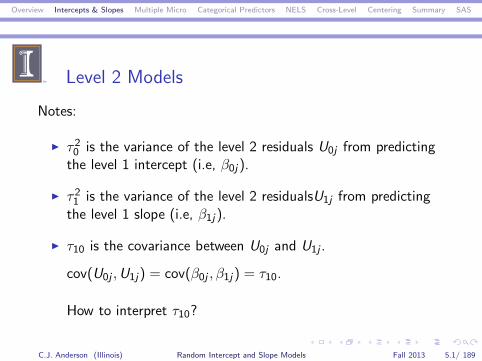
Covariance Parameter Estimates
Standard ZCovariance Parm Subject Estimate Error Value Pr Z
τ00 UN(1,1) id 8.6161 1.0684 8.06 < .0001τ01 UN(2,1) id 0.05041 0.4024 0.13 .9003τ11 UN(2,2) id 0.6782 0.2780 2.44 .0073σ2 Residual 36.7005 0.6257 58.65 < .0001
C.J. Anderson (Illinois) Random Intercept and Slope Models Fall 2013 18.1/ 189

Overview Intercepts & Slopes Multiple Micro Categorical Predictors NELS Cross-Level Centering Summary SAS
Solution for Fixed Effects
StandardEffect Estimate Error DF t Value Pr> |t|
γ00 Intercept 12.6494 0.2437 159 51.91 < .0001γ10 cses 2.1931 0.1278 159 17.15 < .0001
The average regression line (i.e., fixed part of the model):
mathij = 12.6494 + 2.1931(SESij − SESj),
which is almost the same as the random intercept model:
mathij = 12.6494 + 2.1912(SESij − SESj),
C.J. Anderson (Illinois) Random Intercept and Slope Models Fall 2013 19.1/ 189

Overview Intercepts & Slopes Multiple Micro Categorical Predictors NELS Cross-Level Centering Summary SAS
The Estimated Average Regression Line
mathij = 12.65 + 2.19(SESij − SESj)
C.J. Anderson (Illinois) Random Intercept and Slope Models Fall 2013 20.1/ 189

Overview Intercepts & Slopes Multiple Micro Categorical Predictors NELS Cross-Level Centering Summary SAS
The Estimated Group Regression Lines
mathij = 12.65 + 2.19(SESij − SESj) + U0j + U1j(SESij − SESj)
C.J. Anderson (Illinois) Random Intercept and Slope Models Fall 2013 21.1/ 189
Overview Intercepts & Slopes Multiple Micro Categorical Predictors NELS Cross-Level Centering Summary SAS
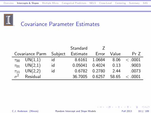
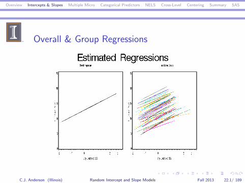
Overall & Group Regressions
C.J. Anderson (Illinois) Random Intercept and Slope Models Fall 2013 22.1/ 189

Overview Intercepts & Slopes Multiple Micro Categorical Predictors NELS Cross-Level Centering Summary SAS
Estimated Variance of Yij (math scores)Random Intercept Model:
var(mathij) = 8.61 + 37.01 = 45.62
Random Intercept and Slope Model
var(mathij) = 8.61 + 2(.05)xij + .68x2ij + 36.70
C.J. Anderson (Illinois) Random Intercept and Slope Models Fall 2013 23.1/ 189

Overview Intercepts & Slopes Multiple Micro Categorical Predictors NELS Cross-Level Centering Summary SAS
Summary & ComparisonRandom
(Baseline) Random interceptNull model intercept and slopeValue SE Value SE Value SE
Fixed Effectsγ00 12.64 .24 12.65 .24 12.65 .24γ10 — — 2.19 .11 2.19 .13
Random Effectsτ20 8.55 1.07 8.61 1.07 8.61 1.07τ10 — — — — .05 .40τ21 — — — — .68 .28σ2 39.15 .66 37.01 .63 36.70 .63
C.J. Anderson (Illinois) Random Intercept and Slope Models Fall 2013 24.1/ 189

Overview Intercepts & Slopes Multiple Micro Categorical Predictors NELS Cross-Level Centering Summary SAS
Example 2: NELS88
◮ Sample N = 23 schools from the full 1003 schools.
◮ Yij , Math achievement is the response/outcome variable.
◮ xij , Homework (time spent doing math homework) is theexplanatory variable.
The models fit to these data:
◮ Null model (Baseline).
◮ Random intercept.
◮ Random intercept and slope models (new one).
C.J. Anderson (Illinois) Random Intercept and Slope Models Fall 2013 25.1/ 189

Overview Intercepts & Slopes Multiple Micro Categorical Predictors NELS Cross-Level Centering Summary SAS
NELS88: Null Model
Dimensions
Covariance Parameters 2Columns in X 1Columns in Z Per Subject 1Subjects 23Max Obs Per Subject 67Observations Used 519Observations Not Used 0Total Observations 519
Convergence criteria met.
C.J. Anderson (Illinois) Random Intercept and Slope Models Fall 2013 26.1/ 189

Overview Intercepts & Slopes Multiple Micro Categorical Predictors NELS Cross-Level Centering Summary SAS
NELS88: Null Model
Covariance Parameter EstimatesStandard ZCov Parm Subject Estimate Error Value Pr Z
Intercept SCHOOL 24.8503 8.4079 2.96 0.0016Residual 81.2374 5.1530 15.77 < .0001
So the intra-class correlation is
ρI =24.8503
24.8503 + 81.2374= .23
C.J. Anderson (Illinois) Random Intercept and Slope Models Fall 2013 27.1/ 189

Overview Intercepts & Slopes Multiple Micro Categorical Predictors NELS Cross-Level Centering Summary SAS
NELS88: Null Model
Solution for the fixed effect:
γ00 = 50.7574
with standard error = 1.1267 (df = 22, t = 45.05, p < .0001).
C.J. Anderson (Illinois) Random Intercept and Slope Models Fall 2013 28.1/ 189

Overview Intercepts & Slopes Multiple Micro Categorical Predictors NELS Cross-Level Centering Summary SAS
NELS88: Random Intercept ModelAdd time spent doing homework,Level 1:
(math)ij = β0j + β1j(homew)ij + Rij
Level 2:
β0j = γ00 + U0j
β1j = γ10
Linear mixed model is
mathij = γ00 + γ10(homew)ij + U0j + Rij
where(
U0j
Rij
)∼ N
((00
),
(τ20 00 σ2
))i .i .d .
C.J. Anderson (Illinois) Random Intercept and Slope Models Fall 2013 29.1/ 189
Overview Intercepts & Slopes Multiple Micro Categorical Predictors NELS Cross-Level Centering Summary SAS
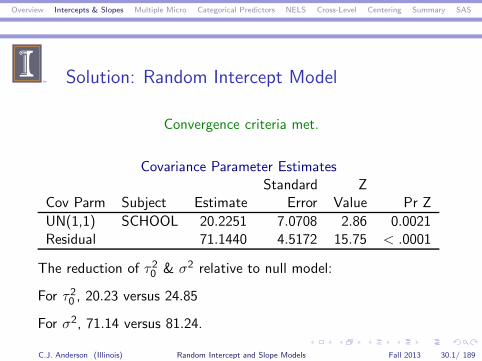
Solution: Random Intercept Model
Convergence criteria met.
Covariance Parameter EstimatesStandard Z
Cov Parm Subject Estimate Error Value Pr Z
UN(1,1) SCHOOL 20.2251 7.0708 2.86 0.0021Residual 71.1440 4.5172 15.75 < .0001
The reduction of τ20 & σ2 relative to null model:
For τ20 , 20.23 versus 24.85
For σ2, 71.14 versus 81.24.
C.J. Anderson (Illinois) Random Intercept and Slope Models Fall 2013 30.1/ 189

Overview Intercepts & Slopes Multiple Micro Categorical Predictors NELS Cross-Level Centering Summary SAS
Solution: Random Intercept Model
Solution for Fixed EffectsStandard
Effect Estimate Error DF t Value Pr > |t|Intercept 46.3494 1.1411 22 40.62 ¡.0001HOMEW 2.4020 0.2768 495 8.68 ¡.0001
The estimated overall regression,
(math)ij = 46.35 + 2.40(homew)ij
C.J. Anderson (Illinois) Random Intercept and Slope Models Fall 2013 31.1/ 189

Overview Intercepts & Slopes Multiple Micro Categorical Predictors NELS Cross-Level Centering Summary SAS
Random Intercept & Slope Model
Question: Is the effect of time spent doing homework differentamong schools?
◮ In some schools, don’t need to rely on homework (tutoring,curriculum, class size, etc.).
◮ The effect of (homew)ij is different in different schools.
◮ Add random slope for time spent doing homework.
C.J. Anderson (Illinois) Random Intercept and Slope Models Fall 2013 32.1/ 189

Overview Intercepts & Slopes Multiple Micro Categorical Predictors NELS Cross-Level Centering Summary SAS
Random Intercept & Slope Model
The model for the NELS88 (N = 23 schools):
Level 1: mathij = β0j + β1j (homew)ij + Rij
Level 2:
β0j = γ00 + U0j
β1j = γ10 + U1j
where
U0j
U1j
Rij
∼ N
(
00
),
τ20 τ10 0τ10 τ21 00 0 σ2
i .i .d .
C.J. Anderson (Illinois) Random Intercept and Slope Models Fall 2013 33.1/ 189

Overview Intercepts & Slopes Multiple Micro Categorical Predictors NELS Cross-Level Centering Summary SAS
Random Intercept & Slope ModelLinear Mixed Model:
(math)ij = γ00 + γ10(homew)ij + U0j + U1j(homew)ij + Rij
Marginal Model:
(math)ij ∼ N (µij , var((math)ij))
whereµij = (γ00 + γ10(homew)ij)
and
var((math)ij) = τ20 + 2τ10(homew)ij + τ21 (homew)2ij + σ2
C.J. Anderson (Illinois) Random Intercept and Slope Models Fall 2013 34.1/ 189

Overview Intercepts & Slopes Multiple Micro Categorical Predictors NELS Cross-Level Centering Summary SAS
Solution: Random Intercept & Slope
Convergence criteria met.
Covariance Parameter EstimatesStandard Z
Cov Parm Subject Estimate Error Value Pr Z
UN(1,1) SCHOOL 59.2439 19.9598 2.97 0.0015UN(2,1) SCHOOL −26.1242 9.8467 −2.65 0.0080UN(2,2) SCHOOL 16.7681 5.8301 2.88 0.0020Residual 53.3000 3.4665 15.38 < .0001
C.J. Anderson (Illinois) Random Intercept and Slope Models Fall 2013 35.1/ 189

Overview Intercepts & Slopes Multiple Micro Categorical Predictors NELS Cross-Level Centering Summary SAS
Solution: Random Intercept & Slope
So
T =
(59.24 −26.12
−26.12 16.77
)
and note that the correlation matrix for U0j and U1j is
Rτ =
(1 −.83
−.83 1
)
C.J. Anderson (Illinois) Random Intercept and Slope Models Fall 2013 36.1/ 189

Overview Intercepts & Slopes Multiple Micro Categorical Predictors NELS Cross-Level Centering Summary SAS
Solution:Random Intercept & Slope
Solution for Fixed EffectsStandard
Effect Estimate Error DF t Value Pr > |t|Intercept 46.3225 1.7190 22 26.95 < .0001HOMEW 1.9870 0.9056 22 2.19 0.0391
The estimated overall regression model is
(math)ij = 46.32 + 1.98(homew)ij
C.J. Anderson (Illinois) Random Intercept and Slope Models Fall 2013 37.1/ 189

Overview Intercepts & Slopes Multiple Micro Categorical Predictors NELS Cross-Level Centering Summary SAS
NELS88 : Summary & Comparison
RandomRandom interceptintercept and slope
Value SE Value SE
Fixed Effectsγ00 46.35 1.4 46.32 1.72γ10 (homew)ij 2.40 .28 1.99 .91
Random Effectsτ20 20.23 7.07 59.24 19.96τ10 −26.12 9.85τ21 16.77 5.83σ2 71.14 4.52 53.30 3.47
C.J. Anderson (Illinois) Random Intercept and Slope Models Fall 2013 38.1/ 189

Overview Intercepts & Slopes Multiple Micro Categorical Predictors NELS Cross-Level Centering Summary SAS
NELS88 : Summary & Comparison
Questions:
1. In the null model τ20 = 24.85 and σ2 = 81.23,why is there a drop in both of these variances when we add(homew)ij to the model?
2. Do we need to include (homew)ij in the random intercept andslope model (i.e., γ10 is small relative to it’s standard error)?
3. Why are the estimates of τ20 and σ2 so different in the randomintercept and slope model relative to the random interceptmodel?
C.J. Anderson (Illinois) Random Intercept and Slope Models Fall 2013 39.1/ 189

Overview Intercepts & Slopes Multiple Micro Categorical Predictors NELS Cross-Level Centering Summary SAS
Question 1School mean time spent doing homework by school...between &within variability.
C.J. Anderson (Illinois) Random Intercept and Slope Models Fall 2013 40.1/ 189

Overview Intercepts & Slopes Multiple Micro Categorical Predictors NELS Cross-Level Centering Summary SAS
Overall Regression. . . in the random intercept and slope model. . .NELS88 (N = 23): Overall (average) regression line — fixedeffects
mathij = 46.32 + 1.99(homew)ij
C.J. Anderson (Illinois) Random Intercept and Slope Models Fall 2013 41.1/ 189

Overview Intercepts & Slopes Multiple Micro Categorical Predictors NELS Cross-Level Centering Summary SAS
Schools’ Regressions. . . in the random intercept and slope model. . .NELS88 (N = 23): Overall (average) regression line — fixedeffects
mathij = 46.32 + 1.99(homew)ij + Uoj + U1j(homew)ij
C.J. Anderson (Illinois) Random Intercept and Slope Models Fall 2013 42.1/ 189

Overview Intercepts & Slopes Multiple Micro Categorical Predictors NELS Cross-Level Centering Summary SAS
Overall and School RegressionsNELS88 (N = 23) Random Intercept & Slope
C.J. Anderson (Illinois) Random Intercept and Slope Models Fall 2013 43.1/ 189

Overview Intercepts & Slopes Multiple Micro Categorical Predictors NELS Cross-Level Centering Summary SAS
Random β0j & β1j versus Random β0jNELS88 (N = 23): Why are τ20 ’s so different?
C.J. Anderson (Illinois) Random Intercept and Slope Models Fall 2013 44.1/ 189

Overview Intercepts & Slopes Multiple Micro Categorical Predictors NELS Cross-Level Centering Summary SAS
Estimated Variance of Math ScoresRandom Intercept Model:
var(Yij) = 20.2251 + 71.1440
Random Intercept and Slope Model:
var(Yij) = 59.2439+2(−26.1242)(hmwk ij)+16.7681(hmwkij)2+53.3000
C.J. Anderson (Illinois) Random Intercept and Slope Models Fall 2013 45.1/ 189

Overview Intercepts & Slopes Multiple Micro Categorical Predictors NELS Cross-Level Centering Summary SAS
Multiple Micro-Level Variables
Mini-outline
1. The model and it’s properties.
2. Example 1: High School & Beyond.
3. Example 2: NELS88.
C.J. Anderson (Illinois) Random Intercept and Slope Models Fall 2013 46.1/ 189
Overview Intercepts & Slopes Multiple Micro Categorical Predictors NELS Cross-Level Centering Summary SAS
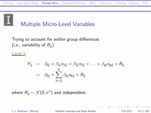
Multiple Micro-Level Variables
Trying to account for within group differences(i.e., variability of Rij).
Level 1:
Yij = β0j + β1jx1ij + β2jx2ij + . . .+ βpjxpij + Rij
= β0j +
p∑
k=1
βkjxkij + Rij
where Rij ∼ N (0, σ2) and independent.
C.J. Anderson (Illinois) Random Intercept and Slope Models Fall 2013 47.1/ 189
Overview Intercepts & Slopes Multiple Micro Categorical Predictors NELS Cross-Level Centering Summary SAS
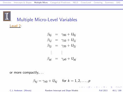
Multiple Micro-Level VariablesLevel 2:
β0j = γ00 + U0j
β1j = γ10 + U1j
β2j = γ20 + U2j
......
βpj = γp0 + Upj
or more compactly,. . .
βkj = γk0 + Ukj for k = 1, 2, . . . , p
C.J. Anderson (Illinois) Random Intercept and Slope Models Fall 2013 48.1/ 189

Overview Intercepts & Slopes Multiple Micro Categorical Predictors NELS Cross-Level Centering Summary SAS
Level 2 Assumptions
where
U0j
U1j
U2j...
Upj
∼ N
000...0
,
τ20 τ10 τ20 . . . τp0τ10 τ21 τ21 . . . τp1τ20 τ21 τ22 . . . τp2...
......
. . ....
τp0 τp1 τp2 . . . τ2p
,
and independent (between macro units) and independent of Rij .
C.J. Anderson (Illinois) Random Intercept and Slope Models Fall 2013 49.1/ 189

Overview Intercepts & Slopes Multiple Micro Categorical Predictors NELS Cross-Level Centering Summary SAS
Linear Mixed Model
Yij = γ00 + γ10x1ij + γ20x2ij + . . . + γp0xpij︸ ︷︷ ︸fixed
+U0j + U1jx1ij + U2jx2ij + . . .+ Upjxpij + Rij︸ ︷︷ ︸random
= γ00 +
p∑
k=1
γk0xkij
︸ ︷︷ ︸+U0j +
p∑
k=1
Ukjxkij + Rij
︸ ︷︷ ︸fixed random
C.J. Anderson (Illinois) Random Intercept and Slope Models Fall 2013 50.1/ 189

Overview Intercepts & Slopes Multiple Micro Categorical Predictors NELS Cross-Level Centering Summary SAS
Linear Mixed Modelin terms of vectors and matrices:
Y1j
Y2j
. . .
Ynj j
=
1 x11j x11j . . . xp1j1 x12j x12j . . . xp2j...
.... . .
......
1 x1nj j x1nj j . . . xpnj j
γ00γ10γ20...
γp0
+
1 x11j x11j . . . xp1j1 x12j x12j . . . xp2j...
.... . .
......
1 x1nj j x1nj j . . . xpnj j
U0j
U1j
U2j...
Upj
+
R1j
R2j...
Rnj j
Yj = XjΓ + ZjUj + Rj
C.J. Anderson (Illinois) Random Intercept and Slope Models Fall 2013 51.1/ 189

Overview Intercepts & Slopes Multiple Micro Categorical Predictors NELS Cross-Level Centering Summary SAS
The Marginal Model
Yij ∼ N (µij , var(Yij))
where
µij = γ00 +
p∑
k=1
γk0xkij
var(Yij) = τ20 + 2
p∑
k=1
τk0xkij +
p∑
k=1
τ2k x2kij + 2
∑
k<l
τklxkijxlij + σ2
In terms of vectors and matrices:
Yj ∼ N((XjΓ), (ZjTZ
′j + σ2I)
).
◮ Where T is the covariance matrix for Uj .◮ Rij ’s and Ukj are independent of each other (i.e., within and
between group residuals are independent)— Assumed this toderive the marginal model.
◮ cov(Yij ,Yij ′) = 0 (i.e, observations from different groups areindependent).
C.J. Anderson (Illinois) Random Intercept and Slope Models Fall 2013 52.1/ 189

Overview Intercepts & Slopes Multiple Micro Categorical Predictors NELS Cross-Level Centering Summary SAS
Example 1: HSB again
Yij = math test scores = response variable.
The xkij ’s:
◮ Student’s SES relative to average of school;
i.e., Group centered SES: (SESij − SESj) . . . numerical
◮ Student’s Gender: genderij = 1 if female, = 0 if male. . . discrete
◮ Student’s Ethnicity: ethnic = 1 if minority, = 0 if not(discrete).
C.J. Anderson (Illinois) Random Intercept and Slope Models Fall 2013 53.1/ 189

Overview Intercepts & Slopes Multiple Micro Categorical Predictors NELS Cross-Level Centering Summary SAS
Example 1: HSB again
The Plan:
1. Add the variables gender and ethnicity as fixed effects.
2. Make the slopes random.
C.J. Anderson (Illinois) Random Intercept and Slope Models Fall 2013 54.1/ 189

Overview Intercepts & Slopes Multiple Micro Categorical Predictors NELS Cross-Level Centering Summary SAS
HSB: Fixed Gender & EthnicityLevel 1:
mathij = β0j + β1j(SESij − SESj) + β2j (gender)ij
+β3j(ethnic)ij + Rij
Level 2:
β0j = γ00 + U0j
β1j = γ10 + U1j
β2j = γ20
β3j = γ30
Assumptions:
U0j
U1j
Rij
∼ N
000
,
τ20 τ10 0τ10 τ21 00 0 σ2
i .i .d .
C.J. Anderson (Illinois) Random Intercept and Slope Models Fall 2013 55.1/ 189

Overview Intercepts & Slopes Multiple Micro Categorical Predictors NELS Cross-Level Centering Summary SAS
HSB: Fixed Gender & Ethnicity
Linear Mixed Model:
mathij = γ00 + γ10(SESij − SESj)
+γ20(gender)ij + γ30(ethnic)ij
+U0j + U1j(SESij − SESj) + Rij
What’s the Marginal Model?
C.J. Anderson (Illinois) Random Intercept and Slope Models Fall 2013 56.1/ 189

Overview Intercepts & Slopes Multiple Micro Categorical Predictors NELS Cross-Level Centering Summary SAS
HSB: Model Information
Data Set WORK.HSBCENTDependent Variable mathachCovariance Structure UnstructuredSubject Effect idEstimation Method MLResidual Variance Method ProfileFixed Effects SEMethod Model-BasedDegrees of Freedom Method Containment
C.J. Anderson (Illinois) Random Intercept and Slope Models Fall 2013 57.1/ 189

Overview Intercepts & Slopes Multiple Micro Categorical Predictors NELS Cross-Level Centering Summary SAS
HSB: Dimensions
Covariance Parameters 4 −→ what are they?Columns in X 4 −→ what are they?Columns in Z Per Subject 2 −→ what are they?Subjects 160Max Obs Per Subject 67Observations Used 7185Observations Not Used 0Total Observations 7185
Convergence criteria met.
C.J. Anderson (Illinois) Random Intercept and Slope Models Fall 2013 58.1/ 189

Overview Intercepts & Slopes Multiple Micro Categorical Predictors NELS Cross-Level Centering Summary SAS
HSB: Covariance Parameters Estimates
Standard ZCov Parm Subject Estimate Error Value Pr Z
UN(1,1) id 6.2575 0.8054 7.77 < .0001UN(2,1) id −0.3014 0.3314 −0.91 0.3631UN(2,2) id 0.4798 0.2521 1.90 0.0285Residual 35.6639 0.6083 58.63 < .0001
C.J. Anderson (Illinois) Random Intercept and Slope Models Fall 2013 59.1/ 189

Overview Intercepts & Slopes Multiple Micro Categorical Predictors NELS Cross-Level Centering Summary SAS
HSB: Solution for Fixed Effects
StandardEffect Estimate Error DF t Value Pr > |t|Intercept 14.1423 0.2350 159 60.18 < .0001cses 1.8945 0.1224 159 15.47 < .0001female −1.2199 0.1643 6863 −7.42 < .0001minority −3.1191 0.2102 6863 −14.84 < .0001
All Look Good.
C.J. Anderson (Illinois) Random Intercept and Slope Models Fall 2013 60.1/ 189

Overview Intercepts & Slopes Multiple Micro Categorical Predictors NELS Cross-Level Centering Summary SAS
HSB: Summary
Null Random Random InterceptModel Intercept and Slope Modelsvalue value value SE value SE
Fixed Effectsγ00 intercept 12.64 12.65 12.65 .24 14.14 .24γ10 cses 2.19 2.19 .13 1.89 .12γ20 female −1.22 .16γ20 minority −3.12 .21
Random Effectsτ20 intercept 8.55 8.61 8.61 1.07 6.26 0.81τ10 .05 .40 −0.30 0.33τ21 cses .68 .28 0.48 0.25σ2 39.15 37.01 36.70 .63 35.66 0.61
C.J. Anderson (Illinois) Random Intercept and Slope Models Fall 2013 61.1/ 189

Overview Intercepts & Slopes Multiple Micro Categorical Predictors NELS Cross-Level Centering Summary SAS
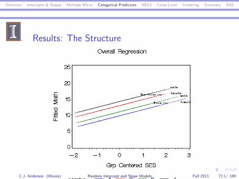
HSB: Interpretation
Random Effects : The larger a school’s intercept (i.e., U0j), thesmaller the school’s slope (i.e., U1j). Is this a valid conclusion??
Fixed Effects: Linear model,
(math)ij = 14.14+1.89(SESij−SESj)−1.22(gender)ij−3.12(ethnic)ij
math)ij =
9.8 + 1.89(SESij − SESj) for minority females
11.02 + 1.89(SESij − SESj) for minority males
12.92 + 1.89(SESij − SESj) for non-minority females
14.14 + 1.89(SESij − SESj) for non-minority males
C.J. Anderson (Illinois) Random Intercept and Slope Models Fall 2013 62.1/ 189

Overview Intercepts & Slopes Multiple Micro Categorical Predictors NELS Cross-Level Centering Summary SAS
HSB: Interpretation (continued)
C.J. Anderson (Illinois) Random Intercept and Slope Models Fall 2013 63.1/ 189

Overview Intercepts & Slopes Multiple Micro Categorical Predictors NELS Cross-Level Centering Summary SAS
Estimated Variance of Math Scores
var(mathij) = τ20 + 2τ10(SESij − SESj) + τ21 (SESij − SESj)2 + σ2
= 6.26 − .60(SESij − SESj) + .48(SESij − SESj)2 + 35.66
Minimum occurs at −τ10
τ21
= .30.48 = .625
C.J. Anderson (Illinois) Random Intercept and Slope Models Fall 2013 64.1/ 189
Overview Intercepts & Slopes Multiple Micro Categorical Predictors NELS Cross-Level Centering Summary SAS
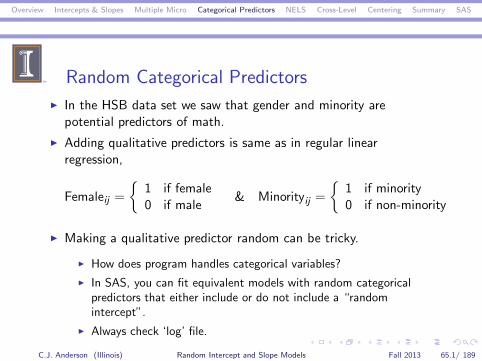
Random Categorical Predictors
◮ In the HSB data set we saw that gender and minority arepotential predictors of math.
◮ Adding qualitative predictors is same as in regular linearregression,
Femaleij =
{1 if female0 if male
& Minorityij =
{1 if minority0 if non-minority
◮ Making a qualitative predictor random can be tricky.
◮ How does program handles categorical variables?
◮ In SAS, you can fit equivalent models with random categoricalpredictors that either include or do not include a “randomintercept”.
◮ Always check ‘log’ file.
C.J. Anderson (Illinois) Random Intercept and Slope Models Fall 2013 65.1/ 189

Overview Intercepts & Slopes Multiple Micro Categorical Predictors NELS Cross-Level Centering Summary SAS
Different Linear Mixed ModelsDefine an additional variable,
Maleij =
{1 if male0 if female
Consider the following models:
(a) mathij = γ00 + γ10(SESij − SESj) + γ11SESj + γ20Femaleij
+u0j + u1jFemaleij + u2jMaleij + σ2
(b) mathij = γ00 + γ10(SESij − SESj) + γ11SESj + γ20Femaleij
+u0j + u1jFemaleij + σ2
(c) mathij = γ00 + γ10(SESij − SESj) + γ11SESj + γ20Femaleij
+u1jFemaleij + u2jMaleij + σ2
C.J. Anderson (Illinois) Random Intercept and Slope Models Fall 2013 66.1/ 189

Overview Intercepts & Slopes Multiple Micro Categorical Predictors NELS Cross-Level Centering Summary SAS
Problem with One of Them
◮ Model (a): In the log file you will find the message
“NOTE: Convergence criteria met but final hessian is notpositive definite”
◮ The hessian is a matrix that is inverted in the estimationalgorithm. If it is “not positive definite”, it cannot beinverted. In this case, it indicates that some effects are(perfectly or highly) correlated.
For males, the intercept is u0j + u2jFor females, the intercept is u0j + u1j
◮ In Model (a), one of the random effects needs to be dropped:u0j , u1j or u2j . These options lead to models (b) and (c).
C.J. Anderson (Illinois) Random Intercept and Slope Models Fall 2013 67.1/ 189

Overview Intercepts & Slopes Multiple Micro Categorical Predictors NELS Cross-Level Centering Summary SAS
HSB: Random Slopes for All
Level 1:
mathij = β0j +β1j (SESij −SESj)+β2j(gender)ij +β3j(ethnic)ij +Rij
where Rij ∼ N (0, σ2).
Level 2:
β0j = γ00 + U0j
β1j = γ10 + U1j
β2j = γ20 + U2j
β3j = γ30 + U3j
where. . .
C.J. Anderson (Illinois) Random Intercept and Slope Models Fall 2013 68.1/ 189

Overview Intercepts & Slopes Multiple Micro Categorical Predictors NELS Cross-Level Centering Summary SAS
HSB: Random Slopes for All
. . . where Uj ∼ N (0,T) i .i .d .
Note: T is (4× 4).
T =
τ20 τ10 τ20 τ30τ10 τ21 τ12 τ31τ20 τ12 τ22 τ32τ30 τ32 τ23 τ23
Linear mixed model:
mathij = γ00 + γ10(SESij − SESj) + γ20(gender)ij + γ30(ethnic)ij
U0j + U1j(SESij − SESj) + U2j(gender)ij + U3j(ethnic)ij
+Rij
C.J. Anderson (Illinois) Random Intercept and Slope Models Fall 2013 69.1/ 189

Overview Intercepts & Slopes Multiple Micro Categorical Predictors NELS Cross-Level Centering Summary SAS
Random Slopes & Discrete VariablesLinear Mixed Model:
mathij = γ00 + γ10(SESij − SESj) + γ20(gender)ij + γ30(ethnic)ij
U0j + U1j(SESij − SESj) + U2j(gender)ij + U3j(ethnic)ij + Rij
Minority Female:
mathij = (γ00 + γ20 + γ30) + γ10(SESij − SESj)
+(U0j + U2j + U3j) + U1j(SESij − SESj ) + Rij
Minority Male:
mathij = (γ00 + γ30) + γ10(SESij − SESj)
+(U0j + U3j) + U1j(SESij − SESj) + Rij
Non-Minority Female:
mathij = (γ00 + γ20) + γ10(SESij − SESj) + (U0j + U2j) + U1j(SESij − SESj) + Rij
Non-Minority Male:
mathij = γ00 + γ10(SESij − SESj) + U0j + U1j(SESij − SESj) + Rij
C.J. Anderson (Illinois) Random Intercept and Slope Models Fall 2013 70.1/ 189

Overview Intercepts & Slopes Multiple Micro Categorical Predictors NELS Cross-Level Centering Summary SAS
Results: Random Slopes for All
Solution for Fixed Effects
Standard tEffect Estimate Error DF Value Pr > |t|Intercept 14.1501 0.2358 159 60.02 < .0001cses 1.8725 0.1197 159 15.64 < .0001female −1.2581 0.1832 122 −6.87 < .0001minority −3.2012 0.2503 135 −12.79 < .0001
C.J. Anderson (Illinois) Random Intercept and Slope Models Fall 2013 71.1/ 189
Overview Intercepts & Slopes Multiple Micro Categorical Predictors NELS Cross-Level Centering Summary SAS
Results: The Structure
C.J. Anderson (Illinois) Random Intercept and Slope Models Fall 2013 72.1/ 189

Overview Intercepts & Slopes Multiple Micro Categorical Predictors NELS Cross-Level Centering Summary SAS
Results: Random Slopes for AllCovariance Parameter Estimates
Standard ZCov Parm Subject Estimate Error Value Pr Z
UN(1,1) id 6.1724 0.9763 6.32 < .0001UN(2,1) id 0.04062 0.3734 0.11 0.9134UN(2,2) id 0.3847 0.2445 1.57 0.0578UN(3,1) id −0.9950 0.6121 −1.63 0.1041UN(3,2) id −0.1339 0.2825 −0.47 0.6354UN(3,3) id 0.8502 0.5588 1.52 0.0640UN(4,1) id 0.9799 0.7496 1.31 0.1911UN(4,2) id −0.5698 0.3675 −1.55 0.1210UN(4,3) id 0.1566 0.6062 0.26 0.7962UN(4,4) id 1.9131 0.9238 2.07 0.0192Residual 35.3088 0.6116 57.73 < .0001
C.J. Anderson (Illinois) Random Intercept and Slope Models Fall 2013 73.1/ 189

Overview Intercepts & Slopes Multiple Micro Categorical Predictors NELS Cross-Level Centering Summary SAS
Results: Random Slopes for All
Covariance Parameter Estimates
T =
intercept cses female minority6.1724 0.04062 −0.9950 0.9799
0.3847 −0.1339 −0.56980.8502 0.1566
1.9131
and σ2 = 35.3088.
C.J. Anderson (Illinois) Random Intercept and Slope Models Fall 2013 74.1/ 189

Overview Intercepts & Slopes Multiple Micro Categorical Predictors NELS Cross-Level Centering Summary SAS
Results: The Stochastic PartRegressions for each school:
C.J. Anderson (Illinois) Random Intercept and Slope Models Fall 2013 75.1/ 189

Overview Intercepts & Slopes Multiple Micro Categorical Predictors NELS Cross-Level Centering Summary SAS
The Stochastic Part (continued)Regressions for each school and gender × ethnicity combination:
C.J. Anderson (Illinois) Random Intercept and Slope Models Fall 2013 76.1/ 189

Overview Intercepts & Slopes Multiple Micro Categorical Predictors NELS Cross-Level Centering Summary SAS
The Stochastic Part (continued)Regressions for two schools – the two most extreme ones in terms of
β1j = γ10 + U1j = 1.8725 + U1j
C.J. Anderson (Illinois) Random Intercept and Slope Models Fall 2013 77.1/ 189

Overview Intercepts & Slopes Multiple Micro Categorical Predictors NELS Cross-Level Centering Summary SAS
The Stochastic Part (continued)Data and Regression lines for one school
C.J. Anderson (Illinois) Random Intercept and Slope Models Fall 2013 78.1/ 189
Overview Intercepts & Slopes Multiple Micro Categorical Predictors NELS Cross-Level Centering Summary SAS
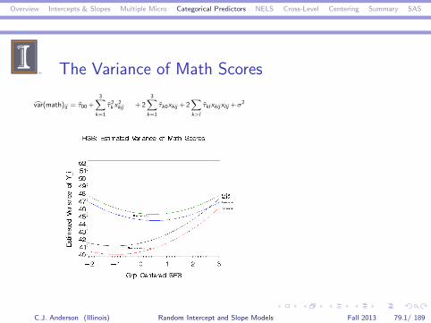
The Variance of Math Scores
var(math)ij = τ00+3∑
k=1
τ2k x2kij +2
3∑
k=1
τk0xkij +2∑
k>l
τklxkijxlij +σ2
C.J. Anderson (Illinois) Random Intercept and Slope Models Fall 2013 79.1/ 189

Overview Intercepts & Slopes Multiple Micro Categorical Predictors NELS Cross-Level Centering Summary SAS
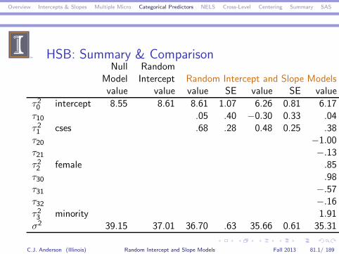
HSB: Summary & Comparison
Fixed EffectsNull Random
Model Intercept Random Intercept and Slopesvalue value value SE value SE value
γ00 intercept 12.64 12.65 12.65 .24 14.14 .24 14.15γ10 cses 2.19 2.19 .13 1.89 .12 1.87γ20 female −1.22 .16 −1.26γ20 minority −3.12 .21 −3.20
Fixed effects are basically the same for group centered SES.
C.J. Anderson (Illinois) Random Intercept and Slope Models Fall 2013 80.1/ 189
Overview Intercepts & Slopes Multiple Micro Categorical Predictors NELS Cross-Level Centering Summary SAS
HSB: Summary & ComparisonNull Random
Model Intercept Random Intercept and Slope Modelsvalue value value SE value SE value
τ20 intercept 8.55 8.61 8.61 1.07 6.26 0.81 6.17τ10 .05 .40 −0.30 0.33 .04τ21 cses .68 .28 0.48 0.25 .38τ20 −1.00τ21 −.13τ22 female .85τ30 .98τ31 −.57τ32 −.16τ23 minority 1.91σ2 39.15 37.01 36.70 .63 35.66 0.61 35.31
C.J. Anderson (Illinois) Random Intercept and Slope Models Fall 2013 81.1/ 189

Overview Intercepts & Slopes Multiple Micro Categorical Predictors NELS Cross-Level Centering Summary SAS
Example 2: NELS (N = 23)◮ homew = time spent doing homework.
◮ minority = white or not (“white” = 1 if white,= 0 otherwise).
◮ sector = public or not (“private” = 1 if private,= 0 public).
So far the models that were fit to the NELS88
◮ Null/baseline model.
◮ Random intercept with homew (time spent doing homework).
◮ Random intercept and slope for homew.
C.J. Anderson (Illinois) Random Intercept and Slope Models Fall 2013 82.1/ 189

Overview Intercepts & Slopes Multiple Micro Categorical Predictors NELS Cross-Level Centering Summary SAS
Example 2: NELS (N = 23)
Models that will be examined are random slope for “homew” and
1. Fixed slopes for minority and sector.
2. Random slope for minority but fixed slope for sector.
3. Random slope for sector but fixed slope for minority.
C.J. Anderson (Illinois) Random Intercept and Slope Models Fall 2013 83.1/ 189
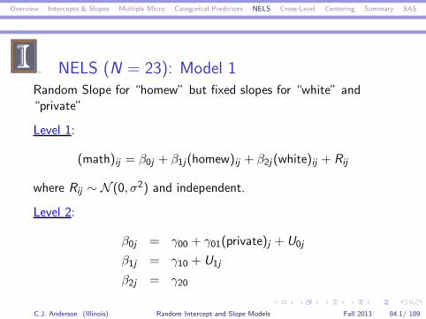
Overview Intercepts & Slopes Multiple Micro Categorical Predictors NELS Cross-Level Centering Summary SAS
NELS (N = 23): Model 1Random Slope for “homew” but fixed slopes for “white” and“private”
Level 1:
(math)ij = β0j + β1j(homew)ij + β2j (white)ij + Rij
where Rij ∼ N (0, σ2) and independent.
Level 2:
β0j = γ00 + γ01(private)j + U0j
β1j = γ10 + U1j
β2j = γ20
C.J. Anderson (Illinois) Random Intercept and Slope Models Fall 2013 84.1/ 189

Overview Intercepts & Slopes Multiple Micro Categorical Predictors NELS Cross-Level Centering Summary SAS
NELS (N = 23): Model 1
. . . where
U0j
U1j
Rij
∼ N
000
,
τ20 τ10 0τ10 τ21 00 0 σ2
Independence within schools for Rij and
Independence between schools for Rij , U0j and U1j .
C.J. Anderson (Illinois) Random Intercept and Slope Models Fall 2013 85.1/ 189

Overview Intercepts & Slopes Multiple Micro Categorical Predictors NELS Cross-Level Centering Summary SAS
NELS (N = 23): Model 1Linear mixed model:
(math)ij = γ00 + γ10(homew)ij + γ20(white)ij + γ01(private)j
+U0j + U1j(homew)ij + Rij
Marginal Model:
(math)ij ∼ N (µ(math), var(math)ij))
where
µ(mathij) = γ00 + γ10(homew)ij + γ20(white)ij + γ01(private)j
var(mathij) = τ20 + τ21 (homew)2ij + 2τ10(homew)ij + σ2.
C.J. Anderson (Illinois) Random Intercept and Slope Models Fall 2013 86.1/ 189

Overview Intercepts & Slopes Multiple Micro Categorical Predictors NELS Cross-Level Centering Summary SAS
Model 1: Fixed/Structural
Solution for Fixed EffectsStandard t
Effect Estimate Error DF Value Pr > |t|Intercept 42.7038 1.8349 21 23.27 < .0001HOMEW 1.9058 0.8819 22 2.16 0.0418WHITE 3.3588 0.9628 472 3.49 0.0005PRIVATE 3.9088 1.7171 472 2.28 0.0233
C.J. Anderson (Illinois) Random Intercept and Slope Models Fall 2013 87.1/ 189

Overview Intercepts & Slopes Multiple Micro Categorical Predictors NELS Cross-Level Centering Summary SAS
Model 1: Random/Stochastic
Covariance Parameter EstimatesStandard Z
Cov Parm Subject Estimate Error Value Pr Z
UN(1,1) SCHOOL 52.2813 18.0535 2.90 0.0019UN(2,1) SCHOOL −25.3464 9.2785 −2.73 0.0063UN(2,2) SCHOOL 15.8384 5.5157 2.87 0.0020Residual 52.6378 3.4288 15.35 < .0001
C.J. Anderson (Illinois) Random Intercept and Slope Models Fall 2013 88.1/ 189

Overview Intercepts & Slopes Multiple Micro Categorical Predictors NELS Cross-Level Centering Summary SAS
Model 1: SummaryRandom Random Intercept
Null Intercept and Slopevalue SE value SE value SE value SE
Fixed Effectsint 50.76 1.13 42.70 1.83 46.32 1.72 42.70 1.83homew 2.40 .28 1.99 .91 1.91 .88white 3.36 .96private 3.91 1.72
Random Effectsτ20 24.85 8.41 20.23 7.07 59.24 19.96 52.28 18.05τ10 −26.12 9.85 −25.35 9.28τ21 16.77 5.83 15.84 5.52σ2 81.24 5.15 71.14 4.52 53.30 3.47 52.64 3.43
C.J. Anderson (Illinois) Random Intercept and Slope Models Fall 2013 89.1/ 189

Overview Intercepts & Slopes Multiple Micro Categorical Predictors NELS Cross-Level Centering Summary SAS
NELS88 (N = 23): Model 2
Random slopes for “homew” and “white”
Level 1: (same)
(math)ij = β0j + β1j(homew)ij + β2j(white)ij + Rij
Level 2:
β0j = γ00 + γ01(private)j + U0j
β1j = γ10 + U1j
β2j = γ20 + U2j
where . . .
C.J. Anderson (Illinois) Random Intercept and Slope Models Fall 2013 90.1/ 189

Overview Intercepts & Slopes Multiple Micro Categorical Predictors NELS Cross-Level Centering Summary SAS
NELS88 (N = 23): Model 2
where Rij ∼ N (0, σ2) and independent, andUj ∼ N (0,T) and independent over schools (i.e., j) and withrespect to Rij ’s.
Note:
Uj =
U0j
U1j
U2j
and T =
τ20 τ10 τ20τ10 τ21 τ12τ20 τ12 τ22
C.J. Anderson (Illinois) Random Intercept and Slope Models Fall 2013 91.1/ 189

Overview Intercepts & Slopes Multiple Micro Categorical Predictors NELS Cross-Level Centering Summary SAS
NELS88 (N = 23): Model 2Linear mixed model:
(math)ij = γ00 + γ10(homew)ij + γ20(white)ij + γ01(private)j
+U0j + U1j(homew)ij + U2j(white)ij + Rij
Marginal Model:
(math)ij ∼ N (µ(math)ij), var(math)ij))
where
µ(math) = γ00 + γ10(homew)ij + γ20(white)ij + γ01(private)ij
var(math)ij) = τ20 + τ21 (homew)2ij + τ22 (white)2ij + 2τ10(homew)ij
+2τ20(white)ij + 2τ12(homew)ij(white)ij + σ2.
C.J. Anderson (Illinois) Random Intercept and Slope Models Fall 2013 92.1/ 189
Overview Intercepts & Slopes Multiple Micro Categorical Predictors NELS Cross-Level Centering Summary SAS
Model 2: Fixed Effects
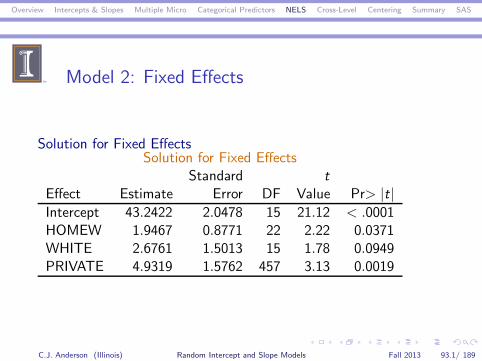
Solution for Fixed EffectsSolution for Fixed Effects
Standard tEffect Estimate Error DF Value Pr> |t|Intercept 43.2422 2.0478 15 21.12 < .0001HOMEW 1.9467 0.8771 22 2.22 0.0371WHITE 2.6761 1.5013 15 1.78 0.0949PRIVATE 4.9319 1.5762 457 3.13 0.0019
C.J. Anderson (Illinois) Random Intercept and Slope Models Fall 2013 93.1/ 189

Overview Intercepts & Slopes Multiple Micro Categorical Predictors NELS Cross-Level Centering Summary SAS
Model 2: Fixed EffectsCovariance Parameter Estimates
Standard ZCov Parm Subject Estimate Error Value Pr Z
τ00 UN(1,1) SCHOOL 64.4072 28.6721 2.25 .0123τ10 UN(2,1) SCHOOL −26.9855 11.3448 −2.38 .0174τ11 UN(2,2) SCHOOL 15.6880 5.4592 2.87 .0020τ20 UN(3,1) SCHOOL −20.1742 19.3586 −1.04 .2974τ21 UN(3,2) SCHOOL 2.7660 7.2729 0.38 .7037τ22 UN(3,3) SCHOOL 24.0397 21.2476 1.13 .1289τsigma Residual 51.1534 3.3845 15.11 < .0001
C.J. Anderson (Illinois) Random Intercept and Slope Models Fall 2013 94.1/ 189
Overview Intercepts & Slopes Multiple Micro Categorical Predictors NELS Cross-Level Centering Summary SAS
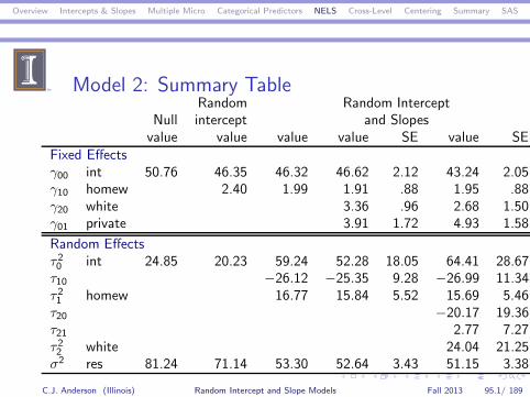
Model 2: Summary TableRandom Random Intercept
Null intercept and Slopesvalue value value value SE value SE
Fixed Effectsγ00 int 50.76 46.35 46.32 46.62 2.12 43.24 2.05γ10 homew 2.40 1.99 1.91 .88 1.95 .88γ20 white 3.36 .96 2.68 1.50γ01 private 3.91 1.72 4.93 1.58
Random Effectsτ20 int 24.85 20.23 59.24 52.28 18.05 64.41 28.67τ10 −26.12 −25.35 9.28 −26.99 11.34τ21 homew 16.77 15.84 5.52 15.69 5.46τ20 −20.17 19.36τ21 2.77 7.27τ22 white 24.04 21.25σ2 res 81.24 71.14 53.30 52.64 3.43 51.15 3.38
C.J. Anderson (Illinois) Random Intercept and Slope Models Fall 2013 95.1/ 189

Overview Intercepts & Slopes Multiple Micro Categorical Predictors NELS Cross-Level Centering Summary SAS
NELS88 (N = 23): Model 3
Random slope for “homew” and “private” but fixed slope for“white”
pause Linear Mixed Model:
(math)ij = γ00 + γ10(homew)ij + γ20(white)ij
+γ30(private)j
+U0j + U1j(homew)ij + U2j(private)j
+Rij
and the usual assumptions for the residuals.
C.J. Anderson (Illinois) Random Intercept and Slope Models Fall 2013 96.1/ 189

Overview Intercepts & Slopes Multiple Micro Categorical Predictors NELS Cross-Level Centering Summary SAS
Model 3: ResultsIn the SAS ouput file:
Convergence criteria met but final hessian is notpositive definite.
◮ What’s wrong with the model we just fit?
◮ We’ll go with Model 2 which has
◮ Random intercept with “private” as an explanatory variable forthe intercept (i.e., level 2).
◮ Random slope for “homew”.
◮ Fixed slope for “white”.
C.J. Anderson (Illinois) Random Intercept and Slope Models Fall 2013 97.1/ 189

Overview Intercepts & Slopes Multiple Micro Categorical Predictors NELS Cross-Level Centering Summary SAS
Model 2: For an average school
mathij = 46.62 + 1.91(homew)ij + 3.35(white)ij + 3.90(private)j
C.J. Anderson (Illinois) Random Intercept and Slope Models Fall 2013 98.1/ 189

Overview Intercepts & Slopes Multiple Micro Categorical Predictors NELS Cross-Level Centering Summary SAS
Model 2: For each of 23 schools
mathij = 46.62 + 1.91(homew)ij + 3.35(white)ij + 3.90(private)j
+U0j + U1j(homew)ij
C.J. Anderson (Illinois) Random Intercept and Slope Models Fall 2013 99.1/ 189

Overview Intercepts & Slopes Multiple Micro Categorical Predictors NELS Cross-Level Centering Summary SAS
Model 2: A Better Look
C.J. Anderson (Illinois) Random Intercept and Slope Models Fall 2013 100.1/ 189

Overview Intercepts & Slopes Multiple Micro Categorical Predictors NELS Cross-Level Centering Summary SAS
Model 2: A Public School
mathij = 46.62 + 1.91(homew)ij + 3.35(white)ij
+U0j + U1j(homew)ij
C.J. Anderson (Illinois) Random Intercept and Slope Models Fall 2013 101.1/ 189

Overview Intercepts & Slopes Multiple Micro Categorical Predictors NELS Cross-Level Centering Summary SAS
Model 2: A Private School
mathij = 46.62 + 1.91(homew)ij + 3.35(white)ij + 3.90(private)j
+U0j + U1j(homew)ij
C.J. Anderson (Illinois) Random Intercept and Slope Models Fall 2013 102.1/ 189

Overview Intercepts & Slopes Multiple Micro Categorical Predictors NELS Cross-Level Centering Summary SAS
Cross-Level Interactions
◮ General model.
◮ Example 1: High School & Beyond.
◮ Example 2: NELS88 (N = 23 schools.
C.J. Anderson (Illinois) Random Intercept and Slope Models Fall 2013 103.1/ 189

Overview Intercepts & Slopes Multiple Micro Categorical Predictors NELS Cross-Level Centering Summary SAS
Cross-Level: A Simple Model
Level 1:Yij = β0j + β1jxij + Rij
where Rij ∼ N (0, σ2).
Level 2:
β0j = γ00 + γ01zj + U0j
β1j = γ10 + γ11zj + U1j
where (U0j
U1j
)∼ N
((00
),
(τ20 τ10τ10 τ21
))
C.J. Anderson (Illinois) Random Intercept and Slope Models Fall 2013 104.1/ 189

Overview Intercepts & Slopes Multiple Micro Categorical Predictors NELS Cross-Level Centering Summary SAS
Cross-Level: A Simple Model
An aside:
We could have different marco variables in the level 2 regressionfor the intercepts and slopes, e.g.,
β0j = γ00 + γ01z1j + U0j
β1j = γ10 + γ11z2j + U1j
C.J. Anderson (Illinois) Random Intercept and Slope Models Fall 2013 105.1/ 189

Overview Intercepts & Slopes Multiple Micro Categorical Predictors NELS Cross-Level Centering Summary SAS
Linear Mixed Model
Yij = γ00 + γ10xij + γ01zj + γ11xijzj︸ ︷︷ ︸+U0j + U1jxij + Rij︸ ︷︷ ︸fixed random
Structural Stochastic
and independent over j and with respect to Rij .
Macro level variables in level 2 regression models for the slopesyield “cross-level interaction” terms in the fixed part of themodel.
C.J. Anderson (Illinois) Random Intercept and Slope Models Fall 2013 106.1/ 189

Overview Intercepts & Slopes Multiple Micro Categorical Predictors NELS Cross-Level Centering Summary SAS
Marginal Model
Yij ∼ N (µij , var(Yij))
where
µij = γ00 + γ10xij + γ01zj + γ11xijzj
andvar(Yij) = τ20 + 2τ10xij + τ21 x
2ij + σ2
C.J. Anderson (Illinois) Random Intercept and Slope Models Fall 2013 107.1/ 189
Overview Intercepts & Slopes Multiple Micro Categorical Predictors NELS Cross-Level Centering Summary SAS
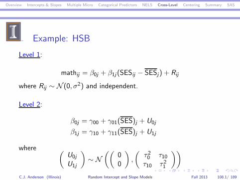
Example: HSB
Level 1:
mathij = β0j + β1j (SESij − SESj) + Rij
where Rij ∼ N (0, σ2) and independent.
Level 2:
β0j = γ00 + γ01(SES)j + U0j
β1j = γ10 + γ11(SES)j + U1j
where (U0j
U1j
)∼ N
((00
),
(τ20 τ10τ10 τ21
))
C.J. Anderson (Illinois) Random Intercept and Slope Models Fall 2013 108.1/ 189

Overview Intercepts & Slopes Multiple Micro Categorical Predictors NELS Cross-Level Centering Summary SAS
HSB ExampleLinear Mixed Model:
Yij = γ00 + γ01(SESj)︸ ︷︷ ︸Intercept
+ (γ10 +︷ ︸︸ ︷γ11SESjModerator
)(SESij − SESj)
︸ ︷︷ ︸Slope
+U0j + U1j(SESij − SESj) + Rij
= γ00 + γ10(SESij − SESj) + γ01(SES)j
+γ11(SESij − SESj)(SES)j
+U0j + U1j(SESij − SESj) + Rij
What’s the marginal model?
C.J. Anderson (Illinois) Random Intercept and Slope Models Fall 2013 109.1/ 189

Overview Intercepts & Slopes Multiple Micro Categorical Predictors NELS Cross-Level Centering Summary SAS
HSB: SAS/MIXED Results
Dimensions
Covariance Parameters 4Columns in X 4Columns in Z Per Subject 2Subjects 160Max Obs Per Subject 67Observations Used 7185Observations Not Used 0Total Observations 7185
Convergence criteria met.
C.J. Anderson (Illinois) Random Intercept and Slope Models Fall 2013 110.1/ 189

Overview Intercepts & Slopes Multiple Micro Categorical Predictors NELS Cross-Level Centering Summary SAS
HSB: Fixed & Random EffectsSolution for Fixed Effects
Standard tEffect Estimate Error Value Pr> |t|Intercept 12.6589 0.1482 85.42 < .0001cses 2.1960 0.1272 17.26 < .0001meanses 5.8700 0.3589 16.36 < .0001cses*meanses 0.2863 0.3169 0.90 0.3663
Covariance Parameter EstimatesStandard Z
Cov Parm Subject Estimate Error Value Pr Z
UN(1,1) id 2.6443 0.3963 6.67 < .0001UN(2,1) id −0.2575 0.2380 −1.08 0.2794UN(2,2) id 0.6496 0.2753 2.36 0.0091Residual 36.7156 0.6261 58.64 < .0001
C.J. Anderson (Illinois) Random Intercept and Slope Models Fall 2013 111.1/ 189

Overview Intercepts & Slopes Multiple Micro Categorical Predictors NELS Cross-Level Centering Summary SAS
Summary of Models for HSB
Null Random RandomModel Intercept Intercept and Slopevalue value value SE value SE
Fixed Effectsγ00 intercept 12.64 12.65 12.65 .24 12.66 .15γ01 cses 2.19 2.19 .13 2.20 .13γ10 meanses 5.87 .36γ11 cses*meanses .29 .32
Random Effectsτ20 intercept 8.55 8.61 8.61 1.07 2.64 .40τ10 .05 .40 −.26 .24τ21 cses .68 .28 .65 .28σ2 39.15 37.01 36.70 .63 36.72 .63
Which/what model might be a good one?C.J. Anderson (Illinois) Random Intercept and Slope Models Fall 2013 112.1/ 189
Overview Intercepts & Slopes Multiple Micro Categorical Predictors NELS Cross-Level Centering Summary SAS
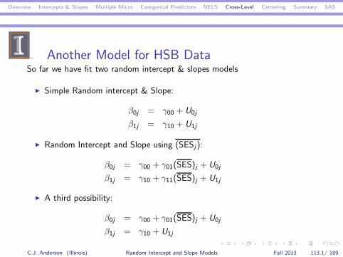
Another Model for HSB DataSo far we have fit two random intercept & slopes models
◮ Simple Random intercept & Slope:
β0j = γ00 + U0j
β1j = γ10 + U1j
◮ Random Intercept and Slope using (SESj):
β0j = γ00 + γ01(SES)j + U0j
β1j = γ10 + γ11(SES)j + U1j
◮ A third possibility:
β0j = γ00 + γ01(SES)j + U0j
β1j = γ10 + U1j
C.J. Anderson (Illinois) Random Intercept and Slope Models Fall 2013 113.1/ 189

Overview Intercepts & Slopes Multiple Micro Categorical Predictors NELS Cross-Level Centering Summary SAS
Model 3 for the HSB Data
Linear Mixed Model:
fixed
mathij =︷ ︸︸ ︷γ00 + γ10(SESij − SESj) + γ01(SES)j
+U0j + U1j(SESij − SESj) + Rij︸ ︷︷ ︸random
or in matrix terms . . .
C.J. Anderson (Illinois) Random Intercept and Slope Models Fall 2013 114.1/ 189

Overview Intercepts & Slopes Multiple Micro Categorical Predictors NELS Cross-Level Centering Summary SAS
Model 3 for the HSB DataLinear Mixed Model in Matrix Terms
math1jmath2j
...mathnj j
=
1 (SES1j − SESj) (SES)j1 (SES2j − SESj) (SES)j...
......
1 (SESnj j − SESj) (SES)j
(γ00γ10γ01
)
+
1 (SES1j − SESj)
1 (SES2j − SESj)...
...
1 (SESnj j − SESj)
(
U0j
U1j
)+
R1j
R2j
...Rnj j
Yj = XjΓ + ZjUj + Rj
C.J. Anderson (Illinois) Random Intercept and Slope Models Fall 2013 115.1/ 189

Overview Intercepts & Slopes Multiple Micro Categorical Predictors NELS Cross-Level Centering Summary SAS
More Linear AlgebraFact: If Y is a vector of random variables,
L and b are vectors of weights (constants),b+ LY is a transformed variable, andΣ is the covariance matrix for Y;
Then Σ(b+LY) = LΣL′.
Another way to write Yj = XjΓ+ ZjUj + Rj ,
Yj = XjΓ+(Zj I
)
Uj
Rj
where I is an (nj × nj) identity matrix.
So for our linear mixed model,
Σyj =(Zj I
)( T 0
0 σ2I
)
Z′
j
I
= ZjTZ
′
j + σ2I
C.J. Anderson (Illinois) Random Intercept and Slope Models Fall 2013 116.1/ 189
Overview Intercepts & Slopes Multiple Micro Categorical Predictors NELS Cross-Level Centering Summary SAS
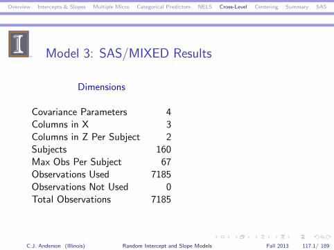
Model 3: SAS/MIXED Results
Dimensions
Covariance Parameters 4Columns in X 3Columns in Z Per Subject 2Subjects 160Max Obs Per Subject 67Observations Used 7185Observations Not Used 0Total Observations 7185
C.J. Anderson (Illinois) Random Intercept and Slope Models Fall 2013 117.1/ 189

Overview Intercepts & Slopes Multiple Micro Categorical Predictors NELS Cross-Level Centering Summary SAS
Model 3: SAS/MIXED Results
Standard ZCov Parm Subject Estimate Error Value Pr Z
UN(1,1) id 2.6445 0.3963 6.67 < .0001UN(2,1) id −0.2596 0.2396 −1.08 0.2787UN(2,2) id 0.6701 0.2766 2.42 0.0077Residual 36.7133 0.6260 58.64 < .0001
StandardEffect Estimate Error t Value Pr > |t|Intercept 12.6588 0.1482 85.41 < .0001cses 2.1912 0.1276 17.17 < .0001meanses 5.8959 0.3577 16.48 < .0001
C.J. Anderson (Illinois) Random Intercept and Slope Models Fall 2013 118.1/ 189

Overview Intercepts & Slopes Multiple Micro Categorical Predictors NELS Cross-Level Centering Summary SAS
Summary of Some of Models for HSBNull Random
Model Intercept Random Intercept and Slopevalue value value SE value SE value
Fixed Effectsγ00 intercept 12.64 12.65 12.65 .24 12.66 .15 12.66γ01 cses 2.19 2.19 .13 2.20 .13 2.19γ10 meanses 5.87 .36 5.90γ11 cses*meanses .29 .32Random Effectsτ20 intercept 8.55 8.61 8.61 1.07 2.64 .40 2.64τ10 .05 .40 −.26 .24 −.26τ21 cses .68 .28 .65 .28 .67σ2 39.15 37.01 36.70 .63 36.72 .63 36.71
mathij = 12.66 + 2.19(SESij − SESj) + 5.90(SES)j
C.J. Anderson (Illinois) Random Intercept and Slope Models Fall 2013 119.1/ 189

Overview Intercepts & Slopes Multiple Micro Categorical Predictors NELS Cross-Level Centering Summary SAS
Model 3: For the Average Schoolwhen SESj = 0, so
mathij = 12.66 + 2.19(SESij − SESj)
C.J. Anderson (Illinois) Random Intercept and Slope Models Fall 2013 120.1/ 189

Overview Intercepts & Slopes Multiple Micro Categorical Predictors NELS Cross-Level Centering Summary SAS
Model 3: For the Average Studentwithin a school when (SESij − SESj) = 0, so
mathij = 12.66 + 5.90(SES)j
C.J. Anderson (Illinois) Random Intercept and Slope Models Fall 2013 121.1/ 189

Overview Intercepts & Slopes Multiple Micro Categorical Predictors NELS Cross-Level Centering Summary SAS
Comparing Average Student & School
C.J. Anderson (Illinois) Random Intercept and Slope Models Fall 2013 122.1/ 189

Overview Intercepts & Slopes Multiple Micro Categorical Predictors NELS Cross-Level Centering Summary SAS
Lots of Micro VariablesThe models can get very complex so here is where theory andsubstantive research questions are very important.
Level 1:
Yij = β0j +
p∑
k=1
βkjxkij + Rij
where Rij ∼ N (0, σ2) i.i.d.
Level 2:β0j = γ00 +
q∑
l=1
γ0lzlj + U0j
β1j = γ10 +
q∑
l=1
γ1lzlj + U1j
......
βpj = γp0 +
q∑
l=1
γplzlj + Upj
where Uj ∼ N (0,T) i.i.d.C.J. Anderson (Illinois) Random Intercept and Slope Models Fall 2013 123.1/ 189

Overview Intercepts & Slopes Multiple Micro Categorical Predictors NELS Cross-Level Centering Summary SAS
Lots of Micro & Macro VariablesLinear Mixed Model:
Yij = γ00 +
p∑
k=1
γk0xkij +
q∑
l=1
γ0lzlj +
p∑
k=1
q∑
l=1
γklxkijzlj
+U0j +
p∑
k=1
Ukjxkij + Rij
where
U0j
U1j...
Upj
Rij
∼ N
00...00
,
τ20 τ10 . . . τp0 0τ10 τ21 . . . τp1 0...
.... . .
... 0τp0 τp1 . . . τ2p 0
0 0 0 0 σ2
i .i .d .
C.J. Anderson (Illinois) Random Intercept and Slope Models Fall 2013 124.1/ 189

Overview Intercepts & Slopes Multiple Micro Categorical Predictors NELS Cross-Level Centering Summary SAS
Lots of Micro & Macro VariablesMarginal Model
Yij ∼ N(µYij
, var(Yij))
where
µYij= γ00 +
p∑
k=1
γk0xkij +
q∑
l=1
γ0lzlj +
p∑
k=1
q∑
l=1
γklxkijzlj
and
var(Yij) = τ20 + 2
p∑
k=1
τk0xkij + 2∑
k 6=l
τklxkijxlij +
p∑
k=1
τ2k x2kij + σ2
C.J. Anderson (Illinois) Random Intercept and Slope Models Fall 2013 125.1/ 189
Overview Intercepts & Slopes Multiple Micro Categorical Predictors NELS Cross-Level Centering Summary SAS
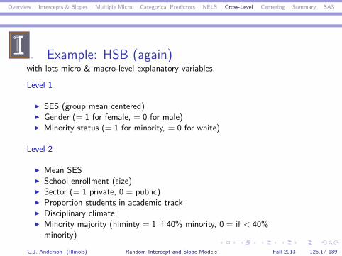
Example: HSB (again)with lots micro & macro-level explanatory variables.
Level 1
◮ SES (group mean centered)◮ Gender (= 1 for female, = 0 for male)◮ Minority status (= 1 for minority, = 0 for white)
Level 2
◮ Mean SES◮ School enrollment (size)◮ Sector (= 1 private, 0 = public)◮ Proportion students in academic track◮ Disciplinary climate◮ Minority majority (himinty = 1 if 40% minority, 0 = if < 40%
minority)
C.J. Anderson (Illinois) Random Intercept and Slope Models Fall 2013 126.1/ 189

Overview Intercepts & Slopes Multiple Micro Categorical Predictors NELS Cross-Level Centering Summary SAS
HSB: Model 1Level 1:
(math)ij = β0j + β1j (cSES)ij + β2j (minority)ij
+β3j(female)ij + Rij
where Rij ∼ N (0, σ2) and i.i.d.
Level 2: Everything into the intercept
β0j = γ00 + γ01(SES)j + γ02(size)j + γ03(sector)j
+γ04(pacad)j + γ05(disclim)j + γ06(himinty)j
+U0j
β1j = γ10 + U1j
β2j = γ20 + U2j
β3j = γ30 + U3j
where Uj ∼ N (0,T).C.J. Anderson (Illinois) Random Intercept and Slope Models Fall 2013 127.1/ 189
Overview Intercepts & Slopes Multiple Micro Categorical Predictors NELS Cross-Level Centering Summary SAS
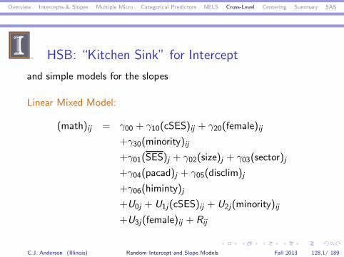
HSB: “Kitchen Sink” for Intercept
and simple models for the slopes
Linear Mixed Model:
(math)ij = γ00 + γ10(cSES)ij + γ20(female)ij
+γ30(minority)ij
+γ01(SES)j + γ02(size)j + γ03(sector)j
+γ04(pacad)j + γ05(disclim)j
+γ06(himinty)j
+U0j + U1j(cSES)ij + U2j(minority)ij
+U3j(female)ij + Rij
C.J. Anderson (Illinois) Random Intercept and Slope Models Fall 2013 128.1/ 189

Overview Intercepts & Slopes Multiple Micro Categorical Predictors NELS Cross-Level Centering Summary SAS
Model 1: SAS/MIXED (edited) Output
Solution for Fixed EffectsStandard t
Effect Estimate Error DF Value Pr> |t|Intercept 11.4831 0.5008 153 22.93 < .0001cSES 1.8867 0.1203 159 15.69 < .0001 Microfemale −1.2814 0.1737 122 −7.38 < .0001minority −3.0752 0.2429 135 −12.66 < .0001
meanses 3.1679 0.4236 6606 7.48 < .0001size 0.000694 0.000209 6606 3.31 .0009 Macrosector 0.8131 0.3776 6606 2.15 .0313pracad 2.7217 0.7952 6606 3.42 .0006disclim −0.4086 0.1753 6606 −2.33 .0198himinty 0.1856 0.3142 6606 0.59 .5548
C.J. Anderson (Illinois) Random Intercept and Slope Models Fall 2013 129.1/ 189

Overview Intercepts & Slopes Multiple Micro Categorical Predictors NELS Cross-Level Centering Summary SAS
Model 1: SAS/MIXED (Edited) OutputCovariance Parameter Estimates
Standard ZCov Parm Estimate Error Value Pr Z
UN(1,1) intercept 1.9323 0.4866 3.97 < .0001UN(2,1) 0.3281 0.2735 1.20 .2303UN(2,2) cSES 0.4029 0.2468 1.63 .0513UN(3,1) −0.8775 0.4183 −2.10 .0359UN(3,2) −0.08297 0.2623 −0.32 .7517UN(3,3) female 0.7350 0.5111 1.44 .0752UN(4,1) −0.2981 0.5291 −0.56 .5732UN(4,2) −0.6821 0.3271 −2.08 .0371UN(4,3) −0.01683 0.5077 −0.03 .9736UN(4,4) minority 1.6198 0.7871 2.06 .0198Residual 35.3381 0.6111 57.83 < .0001
C.J. Anderson (Illinois) Random Intercept and Slope Models Fall 2013 130.1/ 189

Overview Intercepts & Slopes Multiple Micro Categorical Predictors NELS Cross-Level Centering Summary SAS
Model 1: SAS/MIXED Output
The previous slide gave us T (and σ2).
We can also get
Zj TZ′j where j = 1224
Estimated G Matrix:Effect school Col1 Col2 Col3 Col4
Intercept 1224 1.9539 0.3451 −0.8893 −0.3179cSES 1224 0.3451 0.4037 −0.0795 −0.6716female 1224 −0.8893 −0.0795 0.7468 −0.02782minority 1224 −0.3179 −0.6716 −0.02782 1.6014
C.J. Anderson (Illinois) Random Intercept and Slope Models Fall 2013 131.1/ 189

Overview Intercepts & Slopes Multiple Micro Categorical Predictors NELS Cross-Level Centering Summary SAS
HSB Model 2: With Cross-Level Interactions◮ Drop percept minority from intercept model.◮ Retain other macro-variables for intercept model.◮ Add sector to model for a couple of slopes.◮ Level 1:
(math)ij = β0j + β1j (cSES)ij + β2j (minority)ij
+β3j(female)ij + Rij
where Rij ∼ N (0, σ2) and i.i.d.◮ Level 2:
β0j = γ00 + γ01(SES)j + γ02(size)j + γ03(sector)j
+γ04(pacad)j + γ05(disclim)j + U0j
β1j = γ10 + γ11(sector)j + U1j
β2j = γ20 + γ21(sector)j + U2j
β3j = γ30
where Uj ∼ N (0,T).
C.J. Anderson (Illinois) Random Intercept and Slope Models Fall 2013 132.1/ 189

Overview Intercepts & Slopes Multiple Micro Categorical Predictors NELS Cross-Level Centering Summary SAS
HSB Model 2: With Cross Level
Linear Mixed Model
(math)ij = γ00 + γ10(cSES)ij + γ20(female)ij + γ30(minority)ij
+γ01(SES)j + γ02(size)j + γ03(sector)j + γ04(pacad)j
+γ05(disclim)j
+γ11(cSES)ij(sector)j + γ21(minority)ij(sector)j
+U0j + U1j(cSES)ij + U2j(minority)ij + Rij
where (Uj
Rij
)∼ N
((0
0
),
(T 0
0 σ2
)). i .i .d .
C.J. Anderson (Illinois) Random Intercept and Slope Models Fall 2013 133.1/ 189

Overview Intercepts & Slopes Multiple Micro Categorical Predictors NELS Cross-Level Centering Summary SAS
HSB Model 2: SAS/MIXED (edited) OutputSolution for Fixed Effects
Standard tEffect Estimate Error DF Value Pr > |t|Intercept 11.1964 0.4953 154 22.60 < .0001cSES 2.3174 0.1526 158 15.18 < .0001 Microfemale −1.2433 0.1576 6728 −7.89 < .0001minority −3.8520 0.3090 134 −12.47 < .0001meanses 2.8402 0.3925 6728 7.24 < .0001 Macrosize 0.0009 0.0002 6728 4.24 < .0001sector 0.4696 0.3902 6728 1.20 .2289pracad 3.2717 0.7913 6728 4.13 < .0001disclim −0.3555 0.1801 6728 −1.97 .0484cSES*sector −1.0110 0.2277 6728 −4.44 < .0001 Cross-levelminority*sector 1.7885 0.4232 6728 4.23 < .0001
C.J. Anderson (Illinois) Random Intercept and Slope Models Fall 2013 134.1/ 189

Overview Intercepts & Slopes Multiple Micro Categorical Predictors NELS Cross-Level Centering Summary SAS
HSB Model 2: SAS/MIXED Output
Convergence criteria met.Covariance Parameter Estimates
Standard ZCov Parm Estimate Error Value Pr ZUN(1,1) intercept 1.2191 0.2729 4.47 < .0001
UN(2,1) 0.1401 0.1934 0.72 .4687UN(2,2) cSES 0.1634 0.2133 0.77 .2218UN(3,1) −0.0606 0.3554 −0.17 .8646UN(3,2) −0.1427 0.2889 −0.49 .6214UN(3,3) minority 0.7940 0.6684 1.19 .1174Residual 35.4594 0.6081 58.31 < .0001
C.J. Anderson (Illinois) Random Intercept and Slope Models Fall 2013 135.1/ 189

Overview Intercepts & Slopes Multiple Micro Categorical Predictors NELS Cross-Level Centering Summary SAS
HSB Model 3: Refining Model 2
◮ Same Level 1 model.
◮ Note that τ21 (from slope of cSES) and τ22 (from slope ofminority) are small relative to their standard errors —
Later we’ll talk about valid statistical tests of random part ofthe model.
◮ The cross-level interactions between sector and cSES andbetween sector and minority appear to be important.
◮ Let’s make slopes for cSES and minority fixed, but stillinclude explanatory variables for them.
C.J. Anderson (Illinois) Random Intercept and Slope Models Fall 2013 136.1/ 189

Overview Intercepts & Slopes Multiple Micro Categorical Predictors NELS Cross-Level Centering Summary SAS
HSB Model 3: Refining Model 2
The change in the Level 2 model:
β0j = γ00 + γ01(SES)j + γ02(size)j + γ03(sector)j
+γ04(pacad)j + γ05(disclim)j + U0j
β1j = γ10 + γ11(sector)j
β2j = γ20 + γ21(sector)j
β3j = γ30
whereU0j ∼ N (0, τ00)
C.J. Anderson (Illinois) Random Intercept and Slope Models Fall 2013 137.1/ 189

Overview Intercepts & Slopes Multiple Micro Categorical Predictors NELS Cross-Level Centering Summary SAS
HSB Model 3: SAS/MIXED Output
Convergence criteria met.
Covariance Parameter EstimatesStandard Z
Cov Parm Estimate Error Value Pr Z
UN(1,1) 1.3000 0.2423 5.37 < .0001Residual 35.6316 0.6014 59.25 < .0001
C.J. Anderson (Illinois) Random Intercept and Slope Models Fall 2013 138.1/ 189

Overview Intercepts & Slopes Multiple Micro Categorical Predictors NELS Cross-Level Centering Summary SAS
HSB Model 3: SAS/MIXED OutputSolution for Fixed Effects
Standard tEffect Estimate Error DF Value Pr > |t|Intercept 11.2320 0.4968 154 22.61 < .0001cses 2.3167 0.1457 7020 15.90 < .0001 Microfemale −1.2371 0.1575 7020 −7.85 < .0001minority −3.8231 0.2863 7020 −13.35 < .0001meanses 2.8394 0.3856 7020 7.36 < .0001 Macrosize 0.0009 0.0002 7020 4.32 < .0001sector 0.4775 0.3922 7020 1.22 0.2235pracad 3.1853 0.7880 7020 4.04 < .0001disclim −0.3749 0.1793 7020 −2.09 0.0366cses*sector −1.0075 0.2175 7020 −4.63 < .0001 Crossminority*sector 1.7673 0.3862 7020 4.58 < .0001 -level
C.J. Anderson (Illinois) Random Intercept and Slope Models Fall 2013 139.1/ 189

Overview Intercepts & Slopes Multiple Micro Categorical Predictors NELS Cross-Level Centering Summary SAS
Centering Variables
General comments:
◮ The location or centering of explanatory variables determinesthe meaning of the intercept.
◮ In standard linear regression, centering variables leads to thesame model (i.e., same fit, same slope parameters, etc), butwhat about HLM’s?
◮ We’ll investigate various forms of centering under differenttypes of centering (variables in model) and for both RandomIntercept Models and Random Intercept and Slopes Models.
C.J. Anderson (Illinois) Random Intercept and Slope Models Fall 2013 140.1/ 189

Overview Intercepts & Slopes Multiple Micro Categorical Predictors NELS Cross-Level Centering Summary SAS
Types of Centering
◮ None or “Raw Score” (RS): xij
◮ Grand Mean Centered (GMC ): (xij − x)
◮ Group Mean Centered (GpMC ): (xij − xj)
◮ Raw Score + Group Mean (RS + GpM):
xij and xj
◮ Group Mean Centered + Group Mean (GpMC + GPM):
(xij − xj) and xj
C.J. Anderson (Illinois) Random Intercept and Slope Models Fall 2013 141.1/ 189

Overview Intercepts & Slopes Multiple Micro Categorical Predictors NELS Cross-Level Centering Summary SAS
Comparisons in terms of . . .
◮ Statistical Equivalence: Whether models fit data equally well(i.e., same fit statistics, same predictions).
◮ Parameter Equivalence: Whether estimated parameters arethe same or different.
◮ fixed effects (i.e., γ’s)◮ Variances and covariances (i.e., τ ’s & σ2).◮ Estimated covariance matrix for parameter estimates.◮ Estimated correlation matrices for T & Γ.
C.J. Anderson (Illinois) Random Intercept and Slope Models Fall 2013 142.1/ 189

Overview Intercepts & Slopes Multiple Micro Categorical Predictors NELS Cross-Level Centering Summary SAS
Comparisons in terms of . . .
◮ Parameter Stability: On replications of study and/or inclusionof other variables whether the estimated parameters are likelyto be closer to those of the original.
Problem of “Bouncing Beta’s”
◮ Interpretation or the meaning of the intercept and coefficients(i.e., the slopes).
C.J. Anderson (Illinois) Random Intercept and Slope Models Fall 2013 143.1/ 189

Overview Intercepts & Slopes Multiple Micro Categorical Predictors NELS Cross-Level Centering Summary SAS
The Plan
We’ll study random intercept models and then random interceptand slopes models. For each we’ll
◮ Empirically compare models using the NELS88 (N = 23) datawith Yij = math and xij = time spent doing homework.
◮ Determine why we get what we get.
◮ Look at other implications.
◮ Conclude with recommendations.
C.J. Anderson (Illinois) Random Intercept and Slope Models Fall 2013 144.1/ 189
Overview Intercepts & Slopes Multiple Micro Categorical Predictors NELS Cross-Level Centering Summary SAS
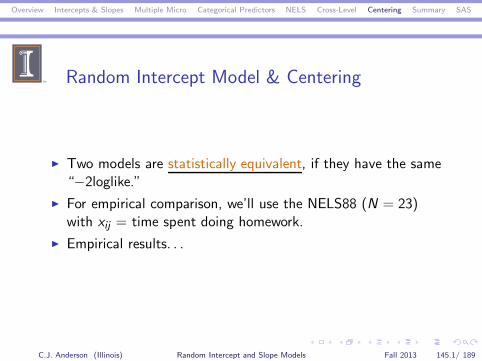
Random Intercept Model & Centering
◮ Two models are statistically equivalent, if they have the same“−2loglike.”
◮ For empirical comparison, we’ll use the NELS88 (N = 23)with xij = time spent doing homework.
◮ Empirical results. . .
C.J. Anderson (Illinois) Random Intercept and Slope Models Fall 2013 145.1/ 189

Overview Intercepts & Slopes Multiple Micro Categorical Predictors NELS Cross-Level Centering Summary SAS
Empirical Results: Statistically Equal
Variable(s) RandomType of Centering in model Intercept
None or “Raw Score” xij 3730.5Grand Mean Centered (xij − x) 3730.5Group mean centered (xij − xj) 3734.4Raw Score + Group Mean xij & xj 3729.6Group Mean Centered+ group mean (xij − xj) & xj 3729.6
C.J. Anderson (Illinois) Random Intercept and Slope Models Fall 2013 146.1/ 189
Overview Intercepts & Slopes Multiple Micro Categorical Predictors NELS Cross-Level Centering Summary SAS
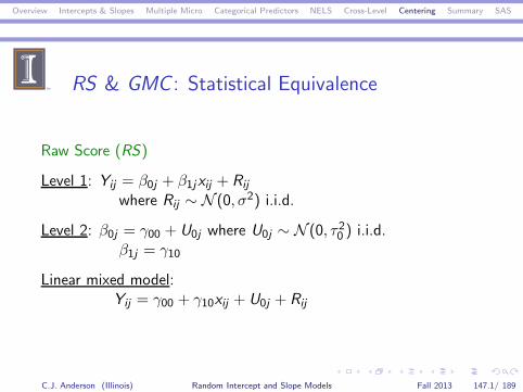
RS & GMC : Statistical Equivalence
Raw Score (RS)
Level 1: Yij = β0j + β1jxij + Rij
where Rij ∼ N (0, σ2) i.i.d.
Level 2: β0j = γ00 + U0j where U0j ∼ N (0, τ20 ) i.i.d.β1j = γ10
Linear mixed model:Yij = γ00 + γ10xij + U0j + Rij
C.J. Anderson (Illinois) Random Intercept and Slope Models Fall 2013 147.1/ 189

Overview Intercepts & Slopes Multiple Micro Categorical Predictors NELS Cross-Level Centering Summary SAS
RS & GMC : Statistical Equivalence
Grand Mean Centered (GMC )
Level 1: Yij = β0j + β1j (xij − x) + Rij
Level 2: β0j = γ00 + U0j
β1j = γ10
Linear mixed model:
Yij = γ00 + γ10(xij − x) + U0j + Rij
(γ00 − γ10x)︸ ︷︷ ︸+ γ10︸︷︷︸ xij + U0j + Rij
= γ00 + γ10xij + U0j + Rij
Same as RSC.J. Anderson (Illinois) Random Intercept and Slope Models Fall 2013 148.1/ 189
Overview Intercepts & Slopes Multiple Micro Categorical Predictors NELS Cross-Level Centering Summary SAS
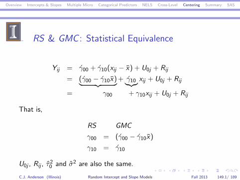
RS & GMC : Statistical Equivalence
Yij = γ00 + γ10(xij − x) + U0j + Rij
= (γ00 − γ10x)︸ ︷︷ ︸+ γ10︸︷︷︸ xij + U0j + Rij
= γ00 + γ10xij + U0j + Rij
That is,
RS GMC
γ00 = (γ00 − γ10x)
γ10 = γ10
U0j , Rij , τ20 and σ2 are also the same.
C.J. Anderson (Illinois) Random Intercept and Slope Models Fall 2013 149.1/ 189

Overview Intercepts & Slopes Multiple Micro Categorical Predictors NELS Cross-Level Centering Summary SAS
RS & GMC : Parameter Equivalence
RS : xij GMC : (xij − x)Parameter value (SE) value (SE)
Fixed effectsintercept γ00 46.3494 (1.14) 51.0840 (1.02)homework γ10 2.4020 (.28) 2.4020 (.28)
Random effectsintercept τ20 20.2251 (7.07) 20.2251 (7.07)residual σ2 71.1440 (4.52) 71.1440 (4.52)
C.J. Anderson (Illinois) Random Intercept and Slope Models Fall 2013 150.1/ 189

Overview Intercepts & Slopes Multiple Micro Categorical Predictors NELS Cross-Level Centering Summary SAS
RS & GMC : Parameter Equivalence
◮ The equivalency
γ00 = (ˆγ00 − ˆγ10x)
46.3493 = 51.0840 − 2.4020(1.9710983)
46.3493 = 46.3493
◮ The SE for the intercept is larger in the raw score model thanit is in the grand mean centered; i.e.,
SE (γ00) = 1.14 versus SE (γ00) = 1.02
◮ The other SE’s are equivalent.
C.J. Anderson (Illinois) Random Intercept and Slope Models Fall 2013 151.1/ 189

Overview Intercepts & Slopes Multiple Micro Categorical Predictors NELS Cross-Level Centering Summary SAS
RS & GMC : Parameter Equivalence
◮ The estimated covariance between the estimated interceptand slope parameters is larger in the raw score case; that is,
ΣΓ =
(1.3022 −.1405−.1405 .07660
)versus Σ
Γ=
(1.0459 .01048.01048 .07660
)
◮ And so is the estimated correlation
RΓ =
(1.0000 −.4449−.4449 1.0000
)versus R
Γ=
(1.0000 −.03702
−.03702 1.0000
)
C.J. Anderson (Illinois) Random Intercept and Slope Models Fall 2013 152.1/ 189

Overview Intercepts & Slopes Multiple Micro Categorical Predictors NELS Cross-Level Centering Summary SAS
RS & GMC : Parameter Equivalence
A little result regarding linear transformations of random variables(vectors):
◮ The linear transformation,
γ00 = (1× ˆγ00) + (−1.9710983 × ˆγ10)
= (1,−1.9710983)
(ˆγ00ˆγ10
)
= L′
(ˆγ00ˆγ10
)
C.J. Anderson (Illinois) Random Intercept and Slope Models Fall 2013 153.1/ 189

Overview Intercepts & Slopes Multiple Micro Categorical Predictors NELS Cross-Level Centering Summary SAS
RS & GMC : Parameter Equivalence
◮ The (estimated) variance for transformed (random) variable,
var(γ00) = L′Σ
ΓL
◮ Applying this to our case:
var(γ00) = (1,−1.9710983)
(1.0459 .01048.01048 .07660
)(1
−1.9710983
)
= 1.3022,
which is exactly what SAS gave us.
◮ Also, SE (γ00) =√1.3022 = 1.14
C.J. Anderson (Illinois) Random Intercept and Slope Models Fall 2013 154.1/ 189

Overview Intercepts & Slopes Multiple Micro Categorical Predictors NELS Cross-Level Centering Summary SAS
RS & GMC
◮ Parameter Stability is not an issue here since there is only oneexplanatory variable.
◮ Interpretation of the intercept:◮ Raw Score:
γ00 equals the value of Yij when xij = 0.◮ Grand mean centering:
γ00 equals the value of Yij when xij = x .
What about the equivalence between RS + GpM andGpMC + GpM?
C.J. Anderson (Illinois) Random Intercept and Slope Models Fall 2013 155.1/ 189

Overview Intercepts & Slopes Multiple Micro Categorical Predictors NELS Cross-Level Centering Summary SAS
RS + GpM and GpMC + GpM
Raw Score plus group mean (RS + GpM):
Level 1: Yij = β∗0j + β∗
1jxij + Rij
where Rij ∼ N (0, σ2) i.i.d.
Level 2: β∗0j = γ∗00 + γ∗01xj + U0j
where U0j ∼ N (0, τ20 ) i.i.d.β∗1j = γ∗10
Linear mixed model:Yij = γ∗00 + γ∗10xij + γ∗01xj + U0j + Rij
C.J. Anderson (Illinois) Random Intercept and Slope Models Fall 2013 156.1/ 189

Overview Intercepts & Slopes Multiple Micro Categorical Predictors NELS Cross-Level Centering Summary SAS
RS + GpM and GpMC + GpM
Group mean centered plus group mean GpMC + GpM
Level 1: Yij = β0j + β1j (xij − xj) + Rij
Level 2: β0j = γ00 + γ01xj + U0j
β1j = γ10
Linear mixed model:
Yij = γ00 + γ10(xij − xj) + γ01xj + U0j + Rij
= γ00︸︷︷︸+ γ10︸︷︷︸ xij + (γ01 − γ10)︸ ︷︷ ︸ xj + U0j + Rij
= γ∗00 + γ∗10xij + γ∗01xj + U0j + Rij
C.J. Anderson (Illinois) Random Intercept and Slope Models Fall 2013 157.1/ 189

Overview Intercepts & Slopes Multiple Micro Categorical Predictors NELS Cross-Level Centering Summary SAS
Parameter Equivalence
Linear mixed model for GpMC + GpM
Yij = γ00 + γ10(xij − xj) + γ01xj + U0j + Rij
= γ00︸︷︷︸+ γ10︸︷︷︸ xij + (γ01 − γ10)︸ ︷︷ ︸ xj + U0j + Rij
= γ∗00 + γ∗10xij + γ∗01xj + U0j + Rij
Same as linear mixed model for RS + GpM whereγ∗00 = γ00γ∗10 = γ10γ∗01 = (γ01 − γ10)
or γ01 = γ∗10 + γ∗01
and U0j , Rij , τ20 , and σ2 are the same.
C.J. Anderson (Illinois) Random Intercept and Slope Models Fall 2013 158.1/ 189
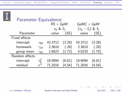
Overview Intercepts & Slopes Multiple Micro Categorical Predictors NELS Cross-Level Centering Summary SAS
Parameter EquivalenceRS + GpM: GpMC + GpM:xij & xj (xij − xj) & xj
Parameter value (SE) value (SE)
Fixed effectsintercept γ00 43.3712 (3.28) 43.3712 (3.28)homework γ10 2.3610 (.28) 2.3610 (.28)group mean γ01 1.6623 (1.72) 4.0233 (1.70)
Random effectsintercept τ20 18.9094 (6.81) 18.9094 (6.81)residual σ2 71.2016 (4.54) 71.2016 (4.54)
C.J. Anderson (Illinois) Random Intercept and Slope Models Fall 2013 159.1/ 189

Overview Intercepts & Slopes Multiple Micro Categorical Predictors NELS Cross-Level Centering Summary SAS
Interpretation of RS + GpM
C.J. Anderson (Illinois) Random Intercept and Slope Models Fall 2013 160.1/ 189

Overview Intercepts & Slopes Multiple Micro Categorical Predictors NELS Cross-Level Centering Summary SAS
Interpretation of RS + GpM
C.J. Anderson (Illinois) Random Intercept and Slope Models Fall 2013 161.1/ 189

Overview Intercepts & Slopes Multiple Micro Categorical Predictors NELS Cross-Level Centering Summary SAS
Parameter Equivalence
between RS + GpM and GpMC + GpM
γ∗01 = ˆγ01 − ˆγ10
1.6623 = 4.0233 − 2.3610
1.6623 = 1.6623
or
ˆγ01 = γ∗10 + γ∗01
4.0233 = 2.3610 + 1.6623
4.0233 = 4.0233
C.J. Anderson (Illinois) Random Intercept and Slope Models Fall 2013 162.1/ 189

Overview Intercepts & Slopes Multiple Micro Categorical Predictors NELS Cross-Level Centering Summary SAS
Parameter Differences
between RS + GpM and GpMC + GpM
◮ SE for the coefficient for the group mean is larger in the rawscore model.
◮ Estimated covariance matrices for fixed
ΣΓ∗ =γ∗00γ∗10γ∗01
10.7376 .0000 −.53139.0000 .07863 −.07863
−.53139 −.07863 2.9746
ΣΓ=
γ00γ10γ01
10.7376 .0000 −.53139.0000 .07863 .0000
−.53139 .0000 2.8960
◮ The transformation leads to this difference.
C.J. Anderson (Illinois) Random Intercept and Slope Models Fall 2013 163.1/ 189

Overview Intercepts & Slopes Multiple Micro Categorical Predictors NELS Cross-Level Centering Summary SAS
Parameter Differences
between RS + GpM and GpMC + GpM
◮ Estimated correlation matrices for fixed
RΓ∗ =γ∗
00
γ∗
10
γ∗
01
(1.0000 .0000 −.9403.0000 1.0000 −.1626
−.9403 −.1626 1.0000
)
versus
RΓ=
γ00γ10γ01
(1.000 .0000 −.9529.0000 1.0000 .0000
−.9529 .0000 1.0000
)
C.J. Anderson (Illinois) Random Intercept and Slope Models Fall 2013 164.1/ 189

Overview Intercepts & Slopes Multiple Micro Categorical Predictors NELS Cross-Level Centering Summary SAS
Parameter Stability
for RS + GpM and GpMC + GpM
◮ The correlation matrix for the explanatory variables:xij , (xij − xj), and xj :
Raw Score xijGrp Mean Center (xij − xj)Grp Mean xj
1.00 .89 .45.89 1.00 .00.45 .00 1.00
◮ Which model is better in terms of parameter stability?
C.J. Anderson (Illinois) Random Intercept and Slope Models Fall 2013 165.1/ 189

Overview Intercepts & Slopes Multiple Micro Categorical Predictors NELS Cross-Level Centering Summary SAS
Interpretation
for RS + GpM and GpMC + GpM
◮ Raw Score + Group Mean Centered (RS + GpM):
Yij = γ∗00 + γ∗10xij + γ∗01xj + U0j + Rij
◮ Group Mean Centered + Group Mean (GpMC + GpM):
Yij = γ00 + γ10(xij − xj) + γ01xj + U0j + Rij
= γ00︸︷︷︸+ γ10︸︷︷︸ xij + (γ01 − γ10)︸ ︷︷ ︸ xj + U0j + Rij
= γ∗00 + γ∗10xij + γ∗01xj + U0j + Rij
C.J. Anderson (Illinois) Random Intercept and Slope Models Fall 2013 166.1/ 189

Overview Intercepts & Slopes Multiple Micro Categorical Predictors NELS Cross-Level Centering Summary SAS
Summary of Models◮ Raw score:
Yij = γ00 + γ10xij + U0j + Rij
◮ Grand mean centered:
Yij = γ00 + γ10(xij − x) + U0j + Rij
◮ Group mean centered:
Yij = γ00 + γ10(xij − xj) + U0j + Rij
◮ Raw score plus group mean:
Yij = γ∗00 + γ∗10xij + γ∗01xj + U0j + Rij
◮ Group mean centered plus group mean:
Yij = γ00 + γ10(xij − xj) + γ01xj + U0j + Rij
C.J. Anderson (Illinois) Random Intercept and Slope Models Fall 2013 167.1/ 189

Overview Intercepts & Slopes Multiple Micro Categorical Predictors NELS Cross-Level Centering Summary SAS
Random Intercept & Slopes
Variable(s) RandomType of Centering in model Intercept
None or Raw score xij 3639.04Grand mean centered (xij − x) 3639.04Group mean centered (xij − xj) 3645.76Raw score + group mean xij & xj 3640.86Group mean centered+ group mean (xij − xj) & xj 3633.89
C.J. Anderson (Illinois) Random Intercept and Slope Models Fall 2013 168.1/ 189

Overview Intercepts & Slopes Multiple Micro Categorical Predictors NELS Cross-Level Centering Summary SAS
Random Intercept & Slopes
Statistical Equivalence:
◮ Only raw score (RS) and grand mean centered (GMC).
◮ Why only these two and why none of the others?
◮ We need to look at the models. . .
C.J. Anderson (Illinois) Random Intercept and Slope Models Fall 2013 169.1/ 189

Overview Intercepts & Slopes Multiple Micro Categorical Predictors NELS Cross-Level Centering Summary SAS
Raw Score (RS)Level 1:
Yij = β0j + β1jxij + Rij ,
where Rij ∼ N (0, σ2) i.i.d.
Level 2:
β0j = γ00 + U0j
β1j = γ10 + U1j ,
where U ∼ N (0,T) i.i.d.
Linear mixed model:
Yij = γ00 + γ10xij + U0j + U1jxij + Rij
C.J. Anderson (Illinois) Random Intercept and Slope Models Fall 2013 170.1/ 189

Overview Intercepts & Slopes Multiple Micro Categorical Predictors NELS Cross-Level Centering Summary SAS
Grand Mean Centered (GMC )
Level 1:Yij = β0j + β1j (xij − x) + Rij
Level 2:
β0j = γ00 + U0j
β1j = γ10 + U1j
Linear mixed model:
Yij = γ00 + γ10(xij − x) + U0j + U1j(xij − x) + Rij
= (γ00 − γ10x)︸ ︷︷ ︸+γ10xij + (U0j − U1j x)︸ ︷︷ ︸+U1jxij + Rij
= γ00 + γ10xij + U0j + U1jxij + RijSame as RS
C.J. Anderson (Illinois) Random Intercept and Slope Models Fall 2013 171.1/ 189

Overview Intercepts & Slopes Multiple Micro Categorical Predictors NELS Cross-Level Centering Summary SAS
Parameter Equivalence
RS GMCxij (xij − x)
Parameter value (SE) value (SE)
Fixed effectsintercept γ00 46.32 (1.72) 50.24 (1.04)homework γ10 1.99 (.91) 1.99 ( .91)
Random effectsintercept τ20 59.24 (19.96) 21.41 (7.16)
τ10 −26.12 (9.85) 6.93 (4.96)homework τ21 16.77 (5.83) 16.77 (5.83)residual σ2 53.30 (3.47) 53.30 (3.47)
C.J. Anderson (Illinois) Random Intercept and Slope Models Fall 2013 172.1/ 189

Overview Intercepts & Slopes Multiple Micro Categorical Predictors NELS Cross-Level Centering Summary SAS
Parameter Equivalence◮ Relationship between parameters
γ00 = ˆγ00 − ˆγx
46.32 = 50.24 − 1.99(1.9710983)
46.32 = 46.32
◮ We have statistical equivalence and know how parameters arerelated, but grand mean centering has an effect on theintercept variance τ20 (& therefore the covariance, τ10).
◮ Intuition regarding thisU0j = U0j − U1j x
More explicitly,
var(U0j) = var(U0j) + var(U1j )x2 − 2cov(U0j , U1j)x
C.J. Anderson (Illinois) Random Intercept and Slope Models Fall 2013 173.1/ 189

Overview Intercepts & Slopes Multiple Micro Categorical Predictors NELS Cross-Level Centering Summary SAS
Comparing Intercept & Slope Models
◮ Raw Score:Yij = γ00 + γ10xij ++U0j + U1jxij + Rij
◮ Grand Mean Centering:Yij = γ00 + γ10(xij − x) + U0j + U1j(xij − x) + Rij
◮ Group Mean Centering:Yij = γ00 + γ10(xij − xj) + U0j + U1j(xij − xj) + Rij
◮ Raw Score plus group mean:Yij = γ∗
00 + γ∗
10xij + γ∗
01xj + U∗
0j + U∗
1jxij + R∗
ij
◮ Group Mean Centering plus group mean:Yij = γ00 + γ10xij + (γ01 + γ10)xj + U0j + U1jxij − U1j xj + Rij
C.J. Anderson (Illinois) Random Intercept and Slope Models Fall 2013 174.1/ 189
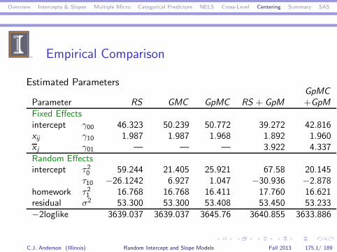
Overview Intercepts & Slopes Multiple Micro Categorical Predictors NELS Cross-Level Centering Summary SAS
Empirical Comparison
Estimated ParametersGpMC
Parameter RS GMC GpMC RS + GpM +GpMFixed Effectsintercept γ00 46.323 50.239 50.772 39.272 42.816xij γ10 1.987 1.987 1.968 1.892 1.960x j γ01 — — — 3.922 4.337Random Effectsintercept τ20 59.244 21.405 25.921 67.58 20.145
τ10 −26.1242 6.927 1.047 −30.936 −2.878homework τ21 16.768 16.768 16.411 17.760 16.621residual σ2 53.300 53.300 53.408 53.450 53.233−2loglike 3639.037 3639.037 3645.76 3640.855 3633.886
C.J. Anderson (Illinois) Random Intercept and Slope Models Fall 2013 175.1/ 189
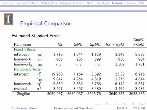
Overview Intercepts & Slopes Multiple Micro Categorical Predictors NELS Cross-Level Centering Summary SAS
Empirical Comparison
Estimated Standard ErrorsGpMC
Parameter RS GMC GpMC RS + GpM +GpMFixed Effectsintercept γ00 1.719 1.044 1.119 3.248 3.273homework γ10 .906 .906 .899 .930 .904
homeworkj γ01 n.a. n.a. n.a. 1.509 1.701Random Effectsintercept τ20 19.960 7.164 8.392 23.32 6.916
τ10 9.847 4.964 4.819 11.275 4.814homework τ21 5.830 5.830 5.758 6.142 5.837residual σ2 3.467 3.467 3.480 3.459 3.485−2loglike 3639.037 3639.037 3645.76 3640.855 3633.886
C.J. Anderson (Illinois) Random Intercept and Slope Models Fall 2013 176.1/ 189
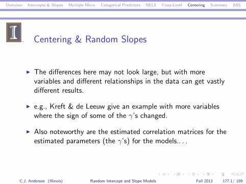
Overview Intercepts & Slopes Multiple Micro Categorical Predictors NELS Cross-Level Centering Summary SAS
Centering & Random Slopes
◮ The differences here may not look large, but with morevariables and different relationships in the data can get vastlydifferent results.
◮ e.g., Kreft & de Leeuw give an example with more variableswhere the sign of some of the γ’s changed.
◮ Also noteworthy are the estimated correlation matrices for theestimated parameters (the γ’s) for the models.. . .
C.J. Anderson (Illinois) Random Intercept and Slope Models Fall 2013 177.1/ 189

Overview Intercepts & Slopes Multiple Micro Categorical Predictors NELS Cross-Level Centering Summary SAS
Centering & Random Slopes
Raw Score plus Group Mean (RS + GpM)
RΓ∗ =
intercept γ00xij γ10xj γ01
(1.0000 -.4450 -.8280-.4450 1.0000 -.0584-.8280 -.0584 1.0000
)
and Group Mean Centering plus Group Mean,
R ˆΓ=
intercept γ00(xij − xj) γ10
xj γ01
(1.0000 -.0355 -.9521-.0355 1.0000 -.0073-.9521 -.0073 1.0000
)
Implications for parameter stability.
C.J. Anderson (Illinois) Random Intercept and Slope Models Fall 2013 178.1/ 189

Overview Intercepts & Slopes Multiple Micro Categorical Predictors NELS Cross-Level Centering Summary SAS
In Sum, With Random Slopes
The location of xij effects
◮ Meaning of the intercept.
◮ Intercept variance.
◮ Covariance between random intercept and random slope.
C.J. Anderson (Illinois) Random Intercept and Slope Models Fall 2013 179.1/ 189

Overview Intercepts & Slopes Multiple Micro Categorical Predictors NELS Cross-Level Centering Summary SAS
Recommendation 1
Snijders & Bosker (p 88):
Generally one should be reluctant to use group-meancentered random slopes models unless there is cleartheory (or an empirical clue) that not in the first placethe absolute score Xij but rather the relative score(Xij − Xj) is related to Yij
C.J. Anderson (Illinois) Random Intercept and Slope Models Fall 2013 180.1/ 189

Overview Intercepts & Slopes Multiple Micro Categorical Predictors NELS Cross-Level Centering Summary SAS
Recommendation 2
Kreft & de Leeuw (p 113–114):
This question cannot be answered on the basis of technicalconsiderations alone.. . . The choice should be made based on theresearcher’s knowledge of the data and the goals of theanalysis.. . . If one decides to center, the only advice we can give. . . is to add the subtracted mean to the model. If this is notdone. . . between effect is not corrected for the mean effect of thecentered first-level explanatory variables. This may be exactly whatone wants, as in growth curve models where the explanatoryvariable is time.
C.J. Anderson (Illinois) Random Intercept and Slope Models Fall 2013 181.1/ 189

Overview Intercepts & Slopes Multiple Micro Categorical Predictors NELS Cross-Level Centering Summary SAS
Recommendation 3
Bryk & Raudenbush (page 28)
Again, the general caveat — be conscious of the choiceof location for each Level-1 predictor because it hasimplications for interpretation of β0j , var(β0j ), and byimplication, all of the covariances involving β0j .
C.J. Anderson (Illinois) Random Intercept and Slope Models Fall 2013 182.1/ 189

Overview Intercepts & Slopes Multiple Micro Categorical Predictors NELS Cross-Level Centering Summary SAS
To Center or NotDepends on
◮ Goals of the analysis, e.g.,
◮ Fitting as much variance as possible.
◮ Substantive theory, e.g.,
Segerstrom, S.C., & Sephton, S.E. (2010).Optimistic Expectancies and Cell-MediatedImmunity : The Role of Positive Affect.Psychological Science, 2, 448–455. DOI:10.1177/0956797610362061
◮ More specific recommendations. . .
C.J. Anderson (Illinois) Random Intercept and Slope Models Fall 2013 183.1/ 189

Overview Intercepts & Slopes Multiple Micro Categorical Predictors NELS Cross-Level Centering Summary SAS
When to Use Raw Scores
or Grand mean centering
◮ If you are more interested in the effects in individuals’performance than in group effects.
e.g., Clustering is a nuisance factor
◮ If group mean centering is a different model that does notmeet requirements of analysis.
C.J. Anderson (Illinois) Random Intercept and Slope Models Fall 2013 184.1/ 189

Overview Intercepts & Slopes Multiple Micro Categorical Predictors NELS Cross-Level Centering Summary SAS
When to use Group Mean Centering
◮ Theory says that individual and group effects are separate.i.e., Two separate models to be tested: one for individual-leveland one for group-level.
◮ Group Mean Centering for technical reasons◮ Smaller correlations between random intercept and random
slope.
◮ Smaller correlations between Level 1 and Level 2 variables andcross-level interactions =⇒ stabilizes model, (coefficients aremore or less independent estimates).
C.J. Anderson (Illinois) Random Intercept and Slope Models Fall 2013 185.1/ 189

Overview Intercepts & Slopes Multiple Micro Categorical Predictors NELS Cross-Level Centering Summary SAS
Summary: Topics/Concepts Covered
◮ Within group dependency accounted for by random effects.◮ Between group differences accounted for by random effects.◮ Central role of variance between and within groups.◮ Regression models for intercept.◮ Effect of adding Level 1 and Level 2 predictors.◮ ICC (for random intercept models)◮ Regression models for intercept and slope.◮ Cross-level interactions occur when models for slopes include
Level 2 measures.◮ HLMs with random slopes (effects) predict heteroscedasticity.◮ Graphing data in various ways can provide insight into possible
effects to consider in developing models for data.. . . much moreon this later.
C.J. Anderson (Illinois) Random Intercept and Slope Models Fall 2013 186.1/ 189
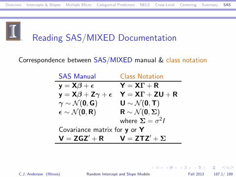
Overview Intercepts & Slopes Multiple Micro Categorical Predictors NELS Cross-Level Centering Summary SAS
Reading SAS/MIXED Documentation
Correspondence between SAS/MIXED manual & class notation
SAS Manual Class Notation
y = Xβ + ǫ Y = XΓ+ R
y = Xβ + Zγ + ǫ Y = XΓ+ ZU+ R
γ ∼ N (0,G) U ∼ N (0,T)ǫ ∼ N (0,R) R ∼ N (0,Σ)
where Σ = σ2ICovariance matrix for y or YV = ZGZ′ + R V = ZTZ′ +Σ
C.J. Anderson (Illinois) Random Intercept and Slope Models Fall 2013 187.1/ 189

Overview Intercepts & Slopes Multiple Micro Categorical Predictors NELS Cross-Level Centering Summary SAS
SAS/MIXED: Random Slopes
◮ Write down the linear mixed model.
◮ The fixed part → MODEL statement.
The COVB and the CORRB options.
◮ The random part → RANDOM statement.
◮ Need to specify TYPE of covariance matrix as an option to theRANDOM statement.
TYPE=un where “un” for unstructured.
C.J. Anderson (Illinois) Random Intercept and Slope Models Fall 2013 188.1/ 189

Overview Intercepts & Slopes Multiple Micro Categorical Predictors NELS Cross-Level Centering Summary SAS
SAS/MIXED: Examples
◮ Go through examples of
◮ Random slopes.
◮ Cross-level interactions.
◮ Note: CPU time and complex and/or poorly specified models.
◮ Computer Lab Session 2: Continue with the USA TIMSS dataset but add some random slopes and a bit of graphics.
C.J. Anderson (Illinois) Random Intercept and Slope Models Fall 2013 189.1/ 189