Random Exemplar Hashing

Tao-Yen Tang, Tzu-Wei Huang, and Hwann-Tzong Chen

Department of Computer ScienceNational Tsing Hua University, Taiwan

Abstract. We present a new method that addresses the problem of approximate nearest neighbor search viapartitioning the feature space. The proposed random exemplar hashing algorithm can be used to generatebinary codes of data to facilitate nearest neighbor search within large datasets. Inspired by the idea of usingan ensemble of classifiers for discriminative learning, we devise an unsupervised learning algorithm to explorethe feature space with respect to randomly selected exemplars. Experimental results on three large datasetsshow that our method outperforms the state-of-the-art, especially on the cases of longer binary codes.

1 Introduction

Nearest neighbor criterion [6] is one of the most popular learning strategies for solving vision problems. Despite itssimplicity, its effectiveness has been shown to be acceptable for various vision applications, especially when high-dimensional distinctive visual features are employed to represent the data [2, 13, 25, 30, 33, 34]. Approximationapproaches such as quantization trees, dimensionality reduction, low-dimensional embedding, and hashing areoften applied to the original high-dimensional data, and more economical coding schemes can be derived tomake the search of nearest neighbors among a large number of data in high-dimensional space more feasible andefficient.

Hashing techniques, e.g. [10, 34] have been widely explored for approximate nearest neighbor search. Theycan achieve fast query speed and only require a limited amount of storage. For example, locality-sensitive hashing(LSH) [10, 15] can offer sub-linear time search via hashing highly similar instances together in a hash table.Regarding data representations, binary codes generated by hashing are often preferred for large-scale search.During query time, since the original feature vectors in the dataset have been converted to binary codes, we mayuse the Hamming distance to retrieve nearest neighbors. The computation of Hamming distance can be made veryfast using bit-wise operations. Hashing-based algorithms are shown to perform well on various large datasets [17,19, 20, 24, 31, 35, 37, 38].

Beyond unsupervised hashing techniques, modern discriminative classifiers have the capability to achievegood performance on supervised image categorization problems. In this work we aim to make use of the discrimi-nating power of classifiers in an unsupervised setting. The mechanism of approximate nearest neighbor search byhashing can be viewed as partitioning the feature space into meaningful regions such that the locality property canbe preserved. The main idea and contribution of our approach is to model and partition the feature space based onlocal data distributions. We propose an unsupervised learning method that explores the feature space with respectto randomly selected exemplars. The method is called random exemplar hashing, in which the randomly selectedexemplars are employed to create an ensemble of classifiers for discriminative learning. We show that our methodis able to generate representative binary hash codes for searching large datasets.

2 Related Work

The basic idea of locality-sensitive hashing (LSH) [10, 15] is to construct hash functions from random projections,which are shown to keep near neighbors together with high probability and thus preserve locality. Since thesuccess of LSH, many hashing techniques have been proposed for approximate nearest neighbor search. Hashingtechniques like LSH are often categorized as data-independent methods because they do not need to learn hashfunctions from training data. Another example is the work of Ji et al. [19]. The basic idea of their approach is toorthogonalize the random projection vectors in batches, and it is theoretically guaranteed that the orthogonalizedrandom projections also provide an unbiased estimate of angular similarity. Yagnik et al. [37] propose the winner-takes-all hashing, which is a sparse embedding method that converts the input feature space into a Hamming spacesuch that the Hamming distance closely resemble the rank similarity.

Data-independent hashing techniques are simple and general, but the majority of hashing techniques try toderive hash codes from data. Semantic hashing [31] uses restricted Boltzmann machines to learn compact binarycodes representing the memory addresses so that semantically similar data are located at nearby addresses andcan be easily compared using the Hamming distance. In a similar spirit, Weiss et al. [36] show that the learning

of compact binary codes can be formulated as an NP-hard graph partitioning problem. They relax the originalproblem, and present the spectral hashing algorithm to solve the relaxed problem. The spectral hashing algorithmcan also handle the problem of out-of-sample extension of spectral methods, and thus can be applied to newinput data easily. More recently, Weiss et al. [35] propose a new multidimensional formulation for learning binarycodes that seek to reconstruct the affinities between data. Unlike spectral hashing whose performance may degradeas the number of bits increases, the optimal code produced by multidimensional spectral hashing is guaranteedto reproduce the affinities between data as the number of bits increases. Spectral hashing mainly assume thatthe input feature vectors are from a Euclidean space. When a better kernel function is available for measuringthe similarities between feature vectors, kernelized locality-sensitive hasing (KLSH) [22] may be used to takeadvantage of the kernel-based similarity measure and derive more effective binary codes for the data.

Several recent methods are also related to our work: The isotropic hashing (IsoHash) algorithm proposed byKong and Li [20] is to learn an orthogonal matrix to rotate the PCA projection matrix. The anchor graph hashing(AGH) algorithm presented by Liu et al. [24] uses anchor graphs to estimate graph Laplacian eigenvectors, and thehash functions are learned by thresholding the lower eigenfunctions of the anchor graph Laplacian. The iterativequantization (ITQ) algorithm proposed by Gong and Lazebnik [11] generates binary hash codes by decidinga rotation of zero-centered data such that the quantization error of mapping the data to the vertices of binaryhypercube can be minimized.

While most embedding algorithms seek to compute binary codes for both the query and the items in thedatabase, some recent research results suggest that binarizing the query is not compulsory, e.g., [3, 8, 12, 16].These asymmetric algorithms show that to binarize the database items but not the query may provide superioraccuracy. The cost of computing the asymmetric distances is generally comparable to the cost of computingsymmetric Hamming distances.

Another way of exploring the feature spaces and encoding the data is to build decision trees based on randomselection of features, such as randomized trees [1, 23] or random forests [4]. Apart from the popular strategiesof tree-structured random feature selection, Rahimi and Recht [29] present two sets of randomized feature mapsthat can be used to approximate various radial basis (shift-invariant) kernels. Rahimi and Recht show that thecombination of the random features with simple linear learning algorithms is comparable to applying kernelmethods (e.g. SVMs) and thus advantageous to dealing with large datasets.

Our work is inspired by the image categorization method of Dai et al. [7]. They use random walk to generatea series of weak training sets. For each WT set, a max-margin classifier is trained to further partition the wholedataset to produce a proximity matrix. The final ensemble proximity matrix derived from the collection of classi-fiers is used to perform spectral clustering for image categorization. In our approach, we randomly choose somedata as exemplars. We obtain the WT sets for the exemplars based on the affinities induced by Gaussian approxi-mation to the feature space, using the method described in [9]. Furthermore, we use the predictions of classifiers toproduce hash codes for searching rather than performing image clustering. Another related method is self-taughthashing (STH) proposed by Zhang et al. [38]. They treat binary codes of training data as binary class labels andtry to learn a set of binary classifiers that can predict the binary codes for new queries. While our method is topartition the feature space defined by the data, the STH method, in a similar sense, is to partition the feature spacethrough the proxy Hamming space defined by precomputed hash codes. Our method also shares similar spirits ofboundary-based representations and hyperplane partitioning methods, of which a detailed survey is available in[32].

3 Random Exemplar Hashing

Many previous algorithms try to find projections that can approximate the original distance by Hamming dis-tance in the Hamming space. We present a new method that addresses the unsupervised learning task of findingprojections through solving small classification problems. The main idea of our method is to partition the high-dimensional feature space by a set of weak classifiers. Our method is fully unsupervised despite the process ofconstructing weak classifiers involves discriminative learning. We do not use the information of class labels orattributes. The weak classifiers are learned from the distributions of data. After combining the decision surfacesof weak classifiers, we can partition the original feature space into convex sets, and the affinities of feature vectorscan be approximately measured according to the binary indexes associated with the convex sets.

Fig. 1 shows the pipeline of our method. At the training stage, we randomly select K ‘exemplars’ from thedataset and set up small classification problems to learn partition functions. We find ‘neighbors’ and ‘foreigners’for each of the exemplars, and build K weak training (WT) sets. The idea of WT sets is similar to [7] but we donot use random walk to collect the WT sets. Each WT set contains M neighboring data points denoted as positivedata andM distant data points denoted as negative data. We then train a weak linear classifier for each WT set andobtain K classifiers. The weak classifiers partition the feature space into convex regions indexed by binary codes.

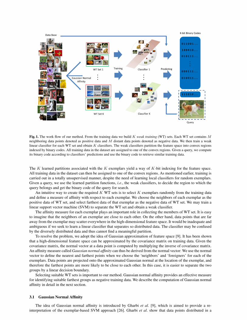
Fig. 1. The work flow of our method. From the training data we build K weak training (WT) sets. Each WT set contains Mneighboring data points denoted as positive data and M distant data points denoted as negative data. We then train a weaklinear classifier for each WT set and obtain K classifiers. The weak classifiers partition the feature space into convex regionsindexed by binary codes. All training data in the dataset are assigned to one of the convex regions. Given a query, we computeits binary code according to classifiers’ predictions and use the binary code to retrieve similar training data.

The K learned partitions associated with the K exemplars yield a way of K-bit indexing for the feature space.All training data in the dataset can then be assigned to one of the convex regions. As mentioned earlier, training iscarried out in a totally unsupervised manner, despite the need of learning local classifiers for random exemplars.Given a query, we use the learned partition functions, i.e., the weak classifiers, to decide the region to which thequery belongs and get the binary code of the query for search.

An intuitive way to create the required K WT sets is to select K exemplars randomly from the training dataand define a measure of affinity with respect to each exemplar. We choose the neighbors of each exemplar as thepositive data of WT set, and select farthest data of that exemplar as the negative data of WT set. We may train alinear support vector machine (SVM) to separate the WT set and obtain a weak classifier.

The affinity measure for each exemplar plays an important role in collecting the members of WT set. It is easyto imagine that the neighbors of an exemplar are close to each other. On the other hand, data points that are faraway from the exemplar may scatter everywhere in the high-dimensional feature space. It would be inadequate andambiguous if we seek to learn a linear classifier that separates so distributed data. The classifier may be confusedby the diversely distributed data and thus cannot find a meaningful partition.

To resolve the problem, we adopt the idea of Gaussian approximation of feature space [9]. It has been shownthat a high-dimensional feature space can be approximated by the covariance matrix on training data. Given thecovariance matrix, the normal vector at a data point is computed by multiplying the inverse of covariance matrix.An affinity measure called Gaussian normal affinity can thus be derived from the normal vector: We use the normalvector to define the nearest and farthest points when we choose the ‘neighbors’ and ‘foreigners’ for each of theexemplars. Data points are projected onto the approximated Gaussian normal at the location of the exemplar, andtherefore the farthest points are more likely to be close to each other. In this case, it is easier to separate the twogroups by a linear decision boundary.

Selecting suitable WT sets is important to our method. Gaussian normal affinity provides an effective measurefor identifying suitable farthest groups as negative training data. We describe the computation of Gaussian normalaffinity in detail in the next section.

3.1 Gaussian Normal Affinity

The idea of Gaussian normal affinity is introduced by Gharbi et al. [9], which is aimed to provide a re-interpretation of the exemplar-based SVM approach [26]. Gharbi et al. show that data points distributed in a

high-dimensional feature space can be approximated by a Gaussian, and the normal to the Gaussian at a givenpoint can be used to rank the affinities between the given point and other points. The normal wx to the Gaussianat the location of exemplar x is thus computed by

wx = Σ−1(x− µ) , (1)

where µ and Σ are the mean and the covariance matrix of the approximated Gaussian. The mean µ is triviallyobtained by µ =

∑i vi/N , where N is the number of training data and {vi|vi ∈ RD, i = 1, . . . , N} are

the feature vectors in the training set. The covariance matrix Σ, which is a D-by-D symmetric matrix, can beestimated as Σ =

∑i(vi − µ)(vi − µ)T /N . Note that we only need to compute µ and Σ once, and they are

applicable for new exemplars as long as the exemplars belong to the same feature space.We may define the Gaussian normal affinity as the closeness measured along the direction of the Gaussian

normal wx. That is, we project feature vectors onto the Gaussian normal wx, and use the projected locationsto decide the neighbors and foreigners with respect to the exemplar x. Gaussian normal affinity is an exemplar-specific function. It measures the distance with respect to the ‘shape’ of feature space and the location of exemplarin the feature space.

Gaussian normal affinity helps to define meaningful negative data for WT sets so that linear classifiers can betrained to partition the feature space. All of our experimental results confirm that using Gaussian normal affinityto choose positive and negative data for weak training is better than using Euclidean distance.

It is worth mentioning that Gaussian normal affinity is only used to build the WT sets during training. Afterwe perform weak training tasks and obtain the ensemble of weak classifiers, we directly apply the classifiers tothe input feature vectors since the classifiers have learned how to partition the feature space.

3.2 Single and Dyadic Exemplar Selection Schemes

Gharbi et al. [9] have shown that, in the high-dimensional feature space, feature vectors tend to lie at the outerhypersurface of the set of all feature vectors. Empirically we also find that the group of neighbors and the group offoreigners chosen by an exemplar according to Gaussian normal affinity often lie far away at the opposite ends ofthe outer hypersurface. As a result, the decision plane learned by a linear SVM tends to pass the center of the set offeature vectors. To explore other possibilities of partitioning the feature space, we also try another way to establishWT sets. Instead of selecting one exemplar for each weak training task, we randomly choose two exemplars andfind the neighbors of each exemplar according to its Gaussian normal affinity function. We then arbitrarily assignthe neighbors of one exemplar as positive data and the neighbors of the other exemplar as negative data, and usesuch a WT set to train a weak classifier. We call this process the dyadic exemplar selection scheme [27] in contrastto our original single exemplar selection scheme. We compare these two schemes in latter experiments and showthat they might perform differently on different datasets.

Besides the single and dyadic exemplar selection schemes, we also come up with a very simple version of ourmethod: Given a WT set of positive and negative data found by the single exemplar selection scheme, we computethe mean of positives and the mean of negatives, and take the hyperplane that is orthogonal to the Gaussian normaland passes the middle point of the two means as the decision plane. By doing so we can obtain a weak classifierwithout training linear SVM.

4 Experiments

We evaluate the proposed method on three commonly used large datasets, and compare our method with severalstate-of-the-art hashing techniques by the performance on those datasets.

4.1 Datasets

Three benchmark datasets are used in our experiments:

1. The MIR-Flickr dataset [14] consists of 25, 000 images downloaded from Flickr through its public API.We represent each image by a 540-dimensional Gist descriptor [28]. We randomly choose 1, 000 imagesas queries, and the remaining 24, 000 images are considered as the database. The ‘ground truth’ for eachquery is defined by the top 5% neighbors measured in Euclidean distance, which is the same setting presentedin [19].

2. The CIFAR-10 dataset [21] consists of 60, 000 images, each of which has a size of 32∗32 pixels. We representeach image as a 320-dimensional Gist descriptor. The dataset contains 10 classes including different kinds ofvehicles and animals. In addition to the true labels provided by the dataset, we also test it with ground truthdefined by Euclidean distance. We follow the setting of [20], which sets the average distance of the 50th

nearest neighbor as a threshold, and every image whose distance to the query is smaller than the threshold isconsidered a true positive.

3. The GIST1M dataset used in [18] contains 500, 000 Gist features for learning, 1, 000 for query, and 1, 000, 000as the database to be searched. The learning set consists of the images extracted from the tiny-image datasetof [34]. The database for search is a medley of the INRIA Holidays images and the Flickr1M used in [17].The ground truth is defined by the first 100 nearest neighbors of each query found by Euclidean distance.

4.2 Evaluation details

We compare our method with several state-of-the-art hashing techniques including LSH [10], SH [36], IsoHash[20], ITQ [11], MDSH [35], and AGH [24]. In all comparisons, we run the available program provided by thoseauthors. For the sake of speed, we replace the k-means step in AGH by random selection of data as anchors.This modification does not influence the performance much, but hugely accelerates their method. For AGH onCIFAR-10 and GIST1M datasets, we set the parameter of the number of anchors as 500 and the parameter of howmany nearest anchors used as 100. For AGH on MIR-Flickr dataset we set these two parameters as 500 and 120,respectively. The bandwidth parameter σ of MDSH for computing the affinity matrix is fixed to 0.4.

In our implementation of the proposed method, we use LIBSVM [5] with linear kernel and set the penaltyparameter C of the error term equal to 350 for both the single and dyadic schemes. Since the number of trainingdata is small, it should be adequate to enforce a larger penalty weight on the error term without increasing thetraining time. The issue of overfitting is also not a concern in our case because our goal of weak training isderiving partition functions rather than solving real classification problems. We have tried different settings on theparameter M regarding the size of WT set (containing M positive data and M negative data). We test the valueof M from M = 10 to M = 40. We find that changes in the value of M within this range do not affect the finalprecision much, and so we simply keep M = 20 for all experiments.

We compute the mean average precision (mAP) and plot the precision-recall curves for the evaluations onMIR-Flickr and CIFAR-10 datasets. For GIST1M dataset, we draw the curve that depicts the number of truepositives versus R nearest neighbors. We evaluate all the methods on each dataset using different bit lengths, from32 bits to 512 bits, except the CIFAR-10 dataset. Since ITQ and IsoHash cannot create more bits than the originalfeature dimensions, we set the largest length to 320 bits for CIFAR-10 dataset.

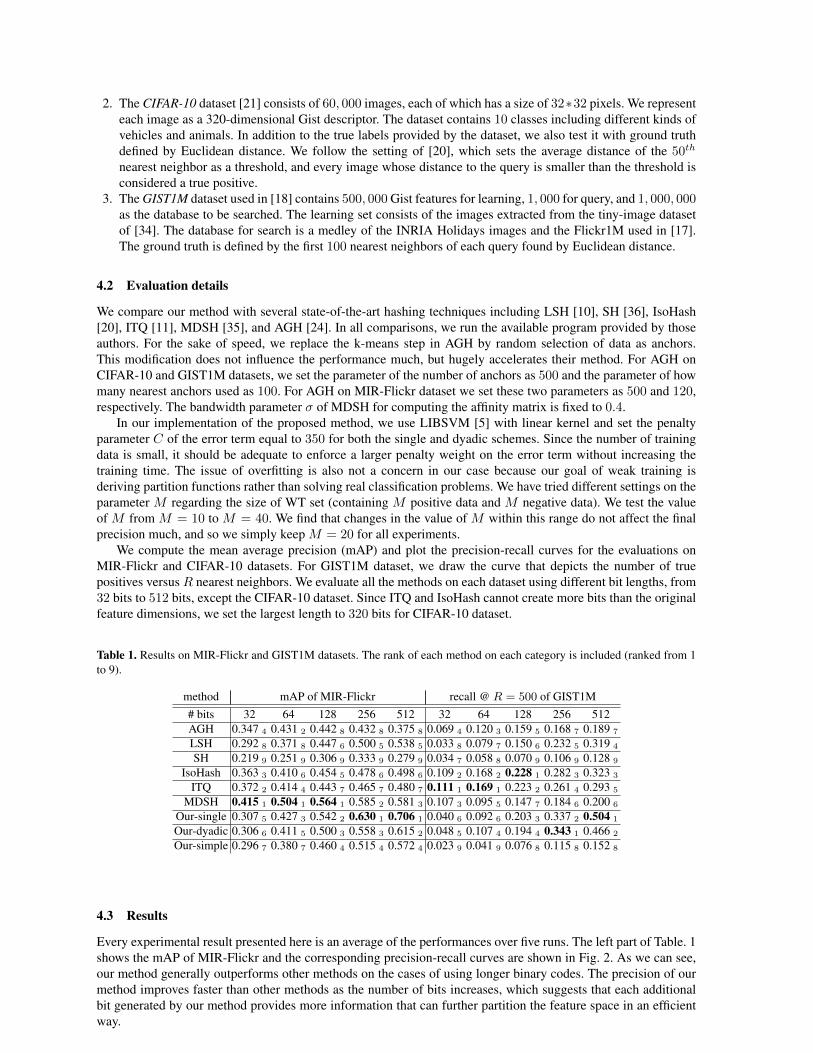
Table 1. Results on MIR-Flickr and GIST1M datasets. The rank of each method on each category is included (ranked from 1to 9).

method mAP of MIR-Flickr recall @ R = 500 of GIST1M# bits 32 64 128 256 512 32 64 128 256 512AGH 0.347 4 0.431 2 0.442 8 0.432 8 0.375 8 0.069 4 0.120 3 0.159 5 0.168 7 0.189 7

LSH 0.292 8 0.371 8 0.447 6 0.500 5 0.538 5 0.033 8 0.079 7 0.150 6 0.232 5 0.319 4

SH 0.219 9 0.251 9 0.306 9 0.333 9 0.279 9 0.034 7 0.058 8 0.070 9 0.106 9 0.128 9

IsoHash 0.363 3 0.410 6 0.454 5 0.478 6 0.498 6 0.109 2 0.168 2 0.228 1 0.282 3 0.323 3

ITQ 0.372 2 0.414 4 0.443 7 0.465 7 0.480 7 0.111 1 0.169 1 0.223 2 0.261 4 0.293 5

MDSH 0.415 1 0.504 1 0.564 1 0.585 2 0.581 3 0.107 3 0.095 5 0.147 7 0.184 6 0.200 6

Our-single 0.307 5 0.427 3 0.542 2 0.630 1 0.706 1 0.040 6 0.092 6 0.203 3 0.337 2 0.504 1

Our-dyadic 0.306 6 0.411 5 0.500 3 0.558 3 0.615 2 0.048 5 0.107 4 0.194 4 0.343 1 0.466 2

Our-simple 0.296 7 0.380 7 0.460 4 0.515 4 0.572 4 0.023 9 0.041 9 0.076 8 0.115 8 0.152 8

4.3 Results

Every experimental result presented here is an average of the performances over five runs. The left part of Table. 1shows the mAP of MIR-Flickr and the corresponding precision-recall curves are shown in Fig. 2. As we can see,our method generally outperforms other methods on the cases of using longer binary codes. The precision of ourmethod improves faster than other methods as the number of bits increases, which suggests that each additionalbit generated by our method provides more information that can further partition the feature space in an efficientway.

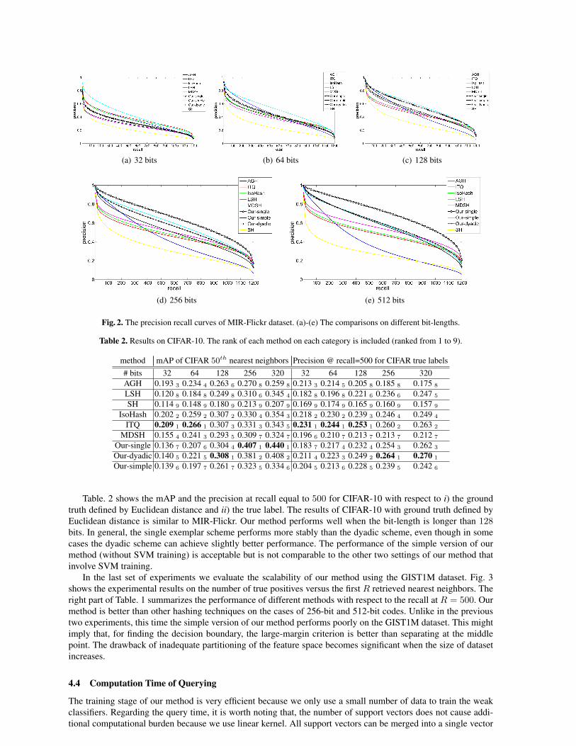
(a) 32 bits (b) 64 bits (c) 128 bits

(d) 256 bits (e) 512 bits

Fig. 2. The precision recall curves of MIR-Flickr dataset. (a)-(e) The comparisons on different bit-lengths.

Table 2. Results on CIFAR-10. The rank of each method on each category is included (ranked from 1 to 9).

method mAP of CIFAR 50th nearest neighbors Precision @ recall=500 for CIFAR true labels# bits 32 64 128 256 320 32 64 128 256 320AGH 0.193 3 0.234 4 0.263 6 0.270 8 0.259 8 0.213 3 0.214 5 0.205 8 0.185 8 0.175 8

LSH 0.120 8 0.184 8 0.249 8 0.310 6 0.345 4 0.182 8 0.196 8 0.221 6 0.236 6 0.247 5

SH 0.114 9 0.148 9 0.180 9 0.213 9 0.207 9 0.169 9 0.174 9 0.165 9 0.160 9 0.157 9

IsoHash 0.202 2 0.259 2 0.307 2 0.330 4 0.354 3 0.218 2 0.230 2 0.239 3 0.246 4 0.249 4

ITQ 0.209 1 0.266 1 0.307 3 0.331 3 0.343 5 0.231 1 0.244 1 0.253 1 0.260 2 0.263 2

MDSH 0.155 4 0.241 3 0.293 5 0.309 7 0.324 7 0.196 6 0.210 7 0.213 7 0.213 7 0.212 7

Our-single 0.136 7 0.207 6 0.304 4 0.407 1 0.440 1 0.183 7 0.217 4 0.232 4 0.254 3 0.262 3

Our-dyadic 0.140 5 0.221 5 0.308 1 0.381 2 0.408 2 0.211 4 0.223 3 0.249 2 0.264 1 0.270 1

Our-simple 0.139 6 0.197 7 0.261 7 0.323 5 0.334 6 0.204 5 0.213 6 0.228 5 0.239 5 0.242 6

Table. 2 shows the mAP and the precision at recall equal to 500 for CIFAR-10 with respect to i) the groundtruth defined by Euclidean distance and ii) the true label. The results of CIFAR-10 with ground truth defined byEuclidean distance is similar to MIR-Flickr. Our method performs well when the bit-length is longer than 128bits. In general, the single exemplar scheme performs more stably than the dyadic scheme, even though in somecases the dyadic scheme can achieve slightly better performance. The performance of the simple version of ourmethod (without SVM training) is acceptable but is not comparable to the other two settings of our method thatinvolve SVM training.

In the last set of experiments we evaluate the scalability of our method using the GIST1M dataset. Fig. 3shows the experimental results on the number of true positives versus the first R retrieved nearest neighbors. Theright part of Table. 1 summarizes the performance of different methods with respect to the recall at R = 500. Ourmethod is better than other hashing techniques on the cases of 256-bit and 512-bit codes. Unlike in the previoustwo experiments, this time the simple version of our method performs poorly on the GIST1M dataset. This mightimply that, for finding the decision boundary, the large-margin criterion is better than separating at the middlepoint. The drawback of inadequate partitioning of the feature space becomes significant when the size of datasetincreases.

4.4 Computation Time of Querying

The training stage of our method is very efficient because we only use a small number of data to train the weakclassifiers. Regarding the query time, it is worth noting that, the number of support vectors does not cause addi-tional computational burden because we use linear kernel. All support vectors can be merged into a single vector

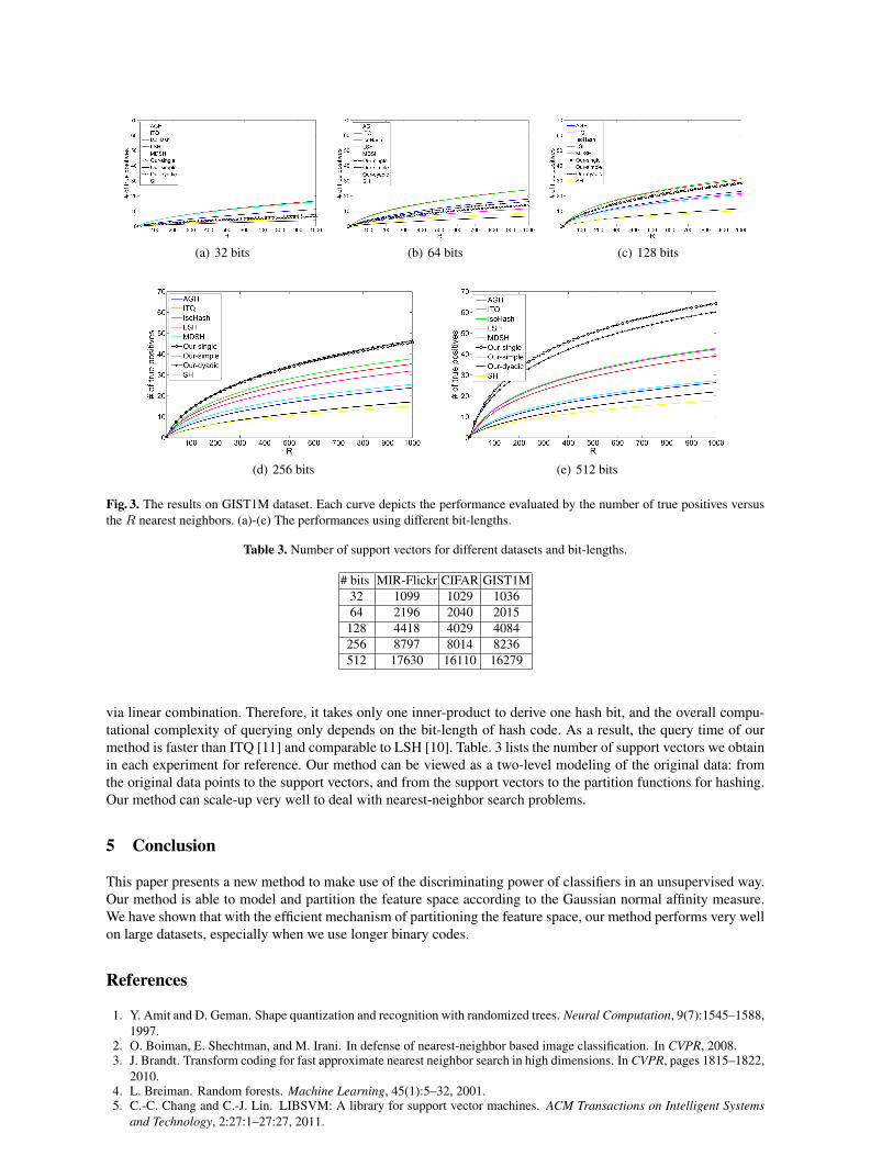
(a) 32 bits (b) 64 bits (c) 128 bits

(d) 256 bits (e) 512 bits

Fig. 3. The results on GIST1M dataset. Each curve depicts the performance evaluated by the number of true positives versusthe R nearest neighbors. (a)-(e) The performances using different bit-lengths.

Table 3. Number of support vectors for different datasets and bit-lengths.

# bits MIR-Flickr CIFAR GIST1M32 1099 1029 103664 2196 2040 2015

128 4418 4029 4084256 8797 8014 8236512 17630 16110 16279

via linear combination. Therefore, it takes only one inner-product to derive one hash bit, and the overall compu-tational complexity of querying only depends on the bit-length of hash code. As a result, the query time of ourmethod is faster than ITQ [11] and comparable to LSH [10]. Table. 3 lists the number of support vectors we obtainin each experiment for reference. Our method can be viewed as a two-level modeling of the original data: fromthe original data points to the support vectors, and from the support vectors to the partition functions for hashing.Our method can scale-up very well to deal with nearest-neighbor search problems.

5 Conclusion

This paper presents a new method to make use of the discriminating power of classifiers in an unsupervised way.Our method is able to model and partition the feature space according to the Gaussian normal affinity measure.We have shown that with the efficient mechanism of partitioning the feature space, our method performs very wellon large datasets, especially when we use longer binary codes.

References

1. Y. Amit and D. Geman. Shape quantization and recognition with randomized trees. Neural Computation, 9(7):1545–1588,1997.

2. O. Boiman, E. Shechtman, and M. Irani. In defense of nearest-neighbor based image classification. In CVPR, 2008.3. J. Brandt. Transform coding for fast approximate nearest neighbor search in high dimensions. In CVPR, pages 1815–1822,

2010.4. L. Breiman. Random forests. Machine Learning, 45(1):5–32, 2001.5. C.-C. Chang and C.-J. Lin. LIBSVM: A library for support vector machines. ACM Transactions on Intelligent Systems

and Technology, 2:27:1–27:27, 2011.

6. T. Cover and P. Hart. Nearest neighbor pattern classification. IEEE Transactions on Information Theory, 13:21–27, 1967.7. D. Dai, M. Prasad, C. Leistner, and L. J. V. Gool. Ensemble partitioning for unsupervised image categorization. In ECCV

(3), pages 483–496, 2012.8. W. Dong, M. Charikar, and K. Li. Asymmetric distance estimation with sketches for similarity search in high-dimensional

spaces. In SIGIR, pages 123–130, 2008.9. M. Gharbi, T. Malisiewicz, S. Paris, and F. Durand. A gaussian approximation of feature space for fast image similarity.

Technical report, Massachusetts Institute of Technology, 2012.10. A. Gionis, P. Indyk, and R. Motwani. Similarity search in high dimensions via hashing. In VLDB, pages 518–529, 1999.11. Y. Gong and S. Lazebnik. Iterative quantization: A procrustean approach to learning binary codes. In CVPR, pages

817–824, 2011.12. A. Gordo and F. Perronnin. Asymmetric distances for binary embeddings. In CVPR, pages 729–736, 2011.13. K. Grauman and T. Darrell. Pyramid match hashing: Sub-linear time indexing over partial correspondences. In CVPR,

2007.14. M. J. Huiskes and M. S. Lew. The mir flickr retrieval evaluation. In MIR ’08: Proceedings of the 2008 ACM International

Conference on Multimedia Information Retrieval, New York, NY, USA, 2008. ACM.15. P. Indyk and R. Motwani. Approximate nearest neighbors: Towards removing the curse of dimensionality. In STOC, pages

604–613, 1998.16. M. Jain, H. Jegou, and P. Gros. Asymmetric hamming embedding: taking the best of our bits for large scale image search.

In ACM Multimedia, pages 1441–1444, 2011.17. H. Jegou, M. Douze, and C. Schmid. Hamming embedding and weak geometric consistency for large scale image search.

In ECCV (1), pages 304–317, 2008.18. H. Jegou, M. Douze, and C. Schmid. Product quantization for nearest neighbor search. IEEE Transactions on Pattern

Analysis & Machine Intelligence, 33(1):117–128, jan 2011.19. J. Ji, J. Li, S. Yan, B. Zhang, and Q. Tian. Super-bit locality-sensitive hashing. In NIPS, pages 108–116, 2012.20. W. Kong and W.-J. Li. Isotropic hashing. In NIPS, pages 1655–1663, 2012.21. A. Krizhevsky. Learning multiple layers of features from tiny images. Technical report, Toronto University, 2009.22. B. Kulis and K. Grauman. Kernelized locality-sensitive hashing for scalable image search. In ICCV, pages 2130–2137,

2009.23. V. Lepetit, P. Lagger, and P. Fua. Randomized trees for real-time keypoint recognition. In CVPR (2), pages 775–781,

2005.24. W. Liu, J. Wang, S. Kumar, and S.-F. Chang. Hashing with graphs. In ICML, pages 1–8, 2011.25. D. G. Lowe. Object recognition from local scale-invariant features. In ICCV, pages 1150–1157, 1999.26. T. Malisiewicz, A. Gupta, and A. A. Efros. Ensemble of exemplar-svms for object detection and beyond. In ICCV, pages

89–96, 2011.27. B. Moghaddam and G. Shakhnarovich. Boosted dyadic kernel discriminants. In NIPS, pages 745–752, 2002.28. A. Oliva and A. Torralba. Modeling the shape of the scene: A holistic representation of the spatial envelope. International

Journal of Computer Vision, 42(3):145–175, 2001.29. A. Rahimi and B. Recht. Random features for large-scale kernel machines. In NIPS, 2007.30. R. Salakhutdinov and G. E. Hinton. Learning a nonlinear embedding by preserving class neighbourhood structure. Journal

of Machine Learning Research - Proceedings Track, 2:412–419, 2007.31. R. Salakhutdinov and G. E. Hinton. Semantic hashing. Int. J. Approx. Reasoning, 50(7):969–978, 2009.32. H. Samet. Foundations of Multidimensional and Metric Data Structures (The Morgan Kaufmann Series in Computer

Graphics and Geometric Modeling). Morgan Kaufmann Publishers Inc., San Francisco, CA, USA, 2005.33. G. Shakhnarovich, T. Darrell, and P. Indyk. Nearest-neighbor methods in learning and vision. IEEE Transactions on

Neural Networks, 19(2):377, 2008.34. A. Torralba, R. Fergus, and W. T. Freeman. 80 million tiny images: A large data set for nonparametric object and scene

recognition. IEEE Trans. Pattern Anal. Mach. Intell., 30(11):1958–1970, 2008.35. Y. Weiss, R. Fergus, and A. Torralba. Multidimensional spectral hashing. In ECCV (5), pages 340–353, 2012.36. Y. Weiss, A. Torralba, and R. Fergus. Spectral hashing. In NIPS, pages 1753–1760, 2008.37. J. Yagnik, D. Strelow, D. A. Ross, and R.-S. Lin. The power of comparative reasoning. In ICCV, pages 2431–2438, 2011.38. D. Zhang, J. Wang, D. Cai, and J. Lu. Self-taught hashing for fast similarity search. In SIGIR, pages 18–25, 2010.