RAMS data collection and failure rate analysis at...

This project has received funding from the European Union’s Horizon 2020 research and innovation programme under grant agreement No 636496

H2020-MG-8.1a-2014

INFRALERT: Linear Infrastructure Efficiency Improvement by Automated Learning and Optimised Predictive Maintenance Techniques

Grant Agreement number: 636496

Work Package WP5. RAMS & LCC models and analysis

Task T5.1. Data compilation at component level T5.2. Failure rate analysis

Revision 5 Due date 30/04/2016

Revision date 10/05/2016 Submission date 29/04/2016

Deliverable type Report

Deliverable leader

CEMOSA

Contributing partners

Fraunhofer IVI, DMA, Universidad de Sevilla, Regens

Dissemination Level

PU Public X

CO Confidential, only for members of the consortium (including the Commission Services)

CI Classified, as referred to in Commission Decision 2001/844/EC.

Deliverable D5.1

RAMS data collection and failure rate analysis at component level

D5.1 – RAMS data collection and failure rate analysis at component level. Revision 5 - 10/05/2016

INFRALERT - 636496 PU

Document status

Revision Date Description

1 21/03/2016 First draft (internal)

2 05/04/2016 Second draft

3 27/04/2016 Third draft

4 29/04/2016 Final

5 10/05/2016 Final (minor corrections)

Status Final



Executive Summary

The deliverable D5.1 belongs to task 5.1 “Data compilation at component level” and partially to task 5.2 “Failure rate analysis”, from WP5, “RAMS & LCC models and analysis”.

The aim of WP5 is to develop a set of algorithms capable of using relevant data collected from the system under study and stored in the Data Farm, and to perform failure rate analysis automatically. This failure rate data will be subsequently used in probabilistic models to derive RAMS&LCC parameters.

This deliverable is intended to provide an overview of RAMS data collection and failure rate analysis, and the identification of the relevant data to perform RAMS&LCC, which usually comprises type and nature of the failure, effects and consequences of the failure, location, environmental conditions, actions taken, repair times and costs, outage cost, date of installations and running time since last failure, etc.

A general description of the relevant data needed in order to accomplish the tasks of WP5, and the tentative output data of this work package will be given.

This deliverable will be subject to revision during the progress of WP5 in order to be in accordance with the rest of the project. Therefore, the information given here should be taken as a first approximation of the final task and might suffer modifications.

This document is organized as follows: in Section 1 the WP5 is contextualised within the INFRALERT eIMS. In Section 2 the objectives of this deliverable are outlined. In Section 3 the RAMS concept is reviewed. Section 4 setups the methodology that will be used to construct the algorithms calculating RAMS and tentative computer tools that could be appropriate to carry out the task. Next, Section 5 deals with the necessary data that will be needed for our calculations and finally in Section 6 the outputs to be obtained as a result of the analysis will be commented.



Table of content

1 Background ........................................................................................................................................... 9

2 Objectives ........................................................................................................................................... 10

3 RAMS concept .................................................................................................................................... 12

4 RAMS methodology ............................................................................................................................ 14

4.1 Basic concepts about the model .................................................................................................. 14

4.2 Analysis of reliability data with covariates .................................................................................. 20

4.3 Model validation .......................................................................................................................... 22

4.4 Software / Tools ........................................................................................................................... 22

5 WP5 Input data ................................................................................................................................... 24

6 WP5 Outputs ...................................................................................................................................... 26

7 Conclusions ......................................................................................................................................... 28

8 Glossary of terms ................................................................................................................................ 29

9 References .......................................................................................................................................... 30



List of tables

Table 1 Relationship between functions defining reliability ................................................................. 18 Table 2 RAMS parameters according to IEC 61703, 2001 ..................................................................... 19 Table 3 Two examples of failure mode record in a DB ......................................................................... 24 Table 4 Files provided for the road demo case ..................................................................................... 26 Table 5 Tentative WO information for the rail demo case ................................................................... 26



List of figures

Figure 1 Components of the INFRALERT eIMS ........................................................................................ 9 Figure 2 Railway system asset hierarchy tree ....................................................................................... 10 Figure 3 Road system asset hierarchy tree ........................................................................................... 10 Figure 4 eIMS architecture .................................................................................................................... 12 Figure 5 Failure episode and definition of times ................................................................................... 15 Figure 6 Schematic course of track quality [13] .................................................................................... 17 Figure 7 Bathtub curve .......................................................................................................................... 17



Abbreviations and acronyms

Abbreviation / Acronym

Description

AFT Accelerate Failure Time

AI Artificial Intelligence

ANOVA Analysis Of Variance

DB Database

DT Down Time

eIMS Expert-based Infrastructure Management System

FOM Force Of Mortality

LCC Life-Cycle Cost

PDF Probability Distribution Function

PH Proportional Hazard

RAMS Reliability, Availability, Maintainability and Safety

ROCOF Rate Of Occurrence Of Failures

RRT Relative Restoration Time

S&C Switches and Crossings

TBF Time Between Failures

TTM Time To Maintain

TTM Time To Maintain

TTR Time To Restore

UT Up Time

WO Work Order

WP Work Package

WT Waiting Time



Mathematical terminology

Throughout this deliverable the following notation will be used:

Capital T denotes the random variable for the survival time, and since T denotes time, then it can only be T>0.

A small letter t denotes any specific value of interest for the random variable capital T. For example, if one is interested in evaluating whether a component survives for more than 5 years, then t=5, and survival means that T may take values larger than 5.

Cumulative density functions are represented in capitals F(t), probability density functions in lower cases f(t). Failure rate is represented with the letter λ(t), and the reliability with R(t).

Letter d stands for a (0,1) random variable indicating either failure (event) or censorship (no event). That is, d=1 for a failure happening during the study period, or d=0 none event happened by the end of the study period.

Vectors are usually represented with capital letters X, for instance the column vector X is:

(

), and its transpose is a row vector ( ), where the set of numbers

x1, …, xn are scalars. The scalar product between two vectors is .



1 Background

INFRALERT aims to develop an expert-based Infrastructure Management System (eIMS) based on artificial intelligence (AI) and optimisation techniques which will rationalise maintenance of linear asset infrastructure systems in favour of increasing its efficiency and cost sustainability, and select optimal strategic decisions on new infrastructure construction.

To reach this goal, one of the objectives is to develop an expert-based toolkit able to perform real-time RAMS&LCC analysis to assess the reliability and life cycle cost of the infrastructure system following probabilistic approaches to allow dealing with uncertainties in intervention planning. The eIMS includes three main subsystems: Data Management, Data Analytics and Decision Support (see Figure 1), and among others, RAMS&LCC analyses will be part of the Data Analytics.

FIGURE 1 COMPONENTS OF THE INFRALERT EIMS

RAMS techniques are a central element in many different application areas, ranging from manufacturing, electrical engineering, transport, and process industry, to nuclear and space industry [1]. Although widely used in the chemical, electronics or nuclear industry, they are new in construction [2]. They have a high potential for applications in transport infrastructure management, but currently there is a lack of standardisation and stated procedures in its implementation [3]. LCC analysis, on the other hand, estimates the most cost-effective option among competing alternatives in maintenance, rehabilitation or construction for a single project and they are common practice in Engineering and Industry. Recently, RAMS&LCC analyses have attracted much attention in the railway sector, with a large number of projects devoted to their development and applications, although their main focus is on LCC methodologies. On the contrary, few experiences of implementing RAMS&LCC approaches are known in the road sector. There is therefore a need for an integrated study of RAMS&LCC to enhance the cost effectiveness of these linear infrastructure systems. Moreover, traditional applications of RAMS&LCC in transport infrastructures have followed a deterministic approach in part due to data availability and computer processing capabilities. The predicting deficiencies inherent of such approaches can be overcome using a probabilistic point of view, where RAMS&LCC are described by probability functions expressing the likelihood that a particular RAMS or LCC state will actually occur.



2 Objectives

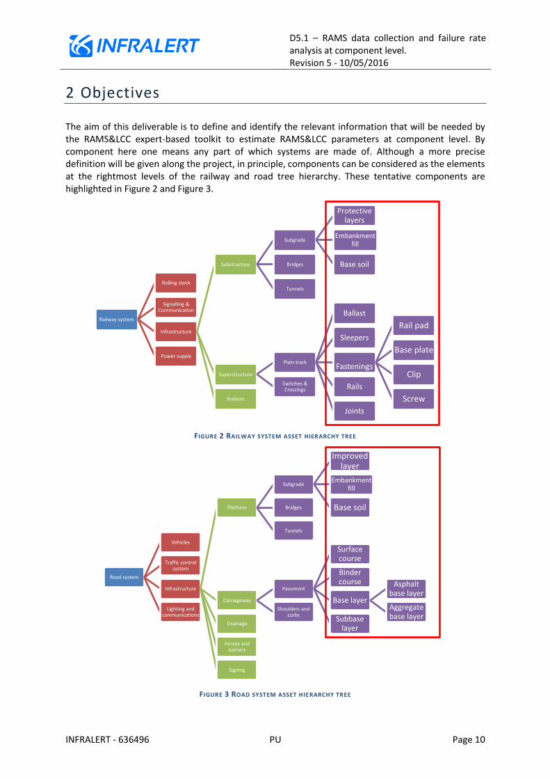
The aim of this deliverable is to define and identify the relevant information that will be needed by the RAMS&LCC expert-based toolkit to estimate RAMS&LCC parameters at component level. By component here one means any part of which systems are made of. Although a more precise definition will be given along the project, in principle, components can be considered as the elements at the rightmost levels of the railway and road tree hierarchy. These tentative components are highlighted in Figure 2 and Figure 3.

FIGURE 2 RAILWAY SYSTEM ASSET HIERARCHY TREE

FIGURE 3 ROAD SYSTEM ASSET HIERARCHY TREE

Railway system

Rolling stock

Signalling & Communication

Infrastructure

Substructure

Subgrade

Protective layers

Embankment fill

Base soil Bridges

Tunnels

Superstructure

Plain track

Ballast

Sleepers

Fastenings

Rail pad

Base plate

Clip

Screw

Rails

Joints

Switches & Crossings

Stations

Power supply

Road system

Vehicles

Traffic control system

Infrastructure

Platform

Subgrade

Improved layer

Embankment fill

Base soil Bridges

Tunnels

Carriageway

Pavement

Surface course

Binder course

Base layer

Asphalt base layer

Aggregate base layer Subbase

layer

Shoulders and curbs

Drainage

Fences and barriers

Signing

Lighting and communications



The basic information needed to calculate RAMS parameters will consist in detailed descriptions of failures in these components previously defined (type, nature, location, time, effects and consequences) as well as a description of the environmental conditions, repair actions taken, their costs, among others.

This information needs to be given in form of data, previously collected and organised in the Data Farm developed in the WP2. In fact, the Data Farm will provide a set of failure occurrences at component level as inputs to the RAMS&LCC expert-based toolkit. Furthermore, the output parameters obtained in the RAMS&LCC simulation will be inputs used by the Smart Decision Support expert-based toolkit later on.

In the next sections, a general description of RAMS parameters at component level, based on its common and widely used mathematical formulation in Reliability Engineering [4], [5], [6] is provided. The required inputs to calculate these RAMS parameters as well as the way they are usually collected are also outlined. Finally, the possible outputs data that will be forwarded to the Smart Decision Support expert-based toolkit are presented.



3 RAMS concept

As shown in Figure 1, RAMS analysis is at the core of the INFRALERT concept. The expert-based Infrastructure Management System (eIMS) includes a collection of toolkits (see Figure 4 on eIMS architecture) and RAMS analysis is one of them. This report defines the basis of INFRALERT RAMS analysis and its interactions with other modules in the eIMS. This section introduces the RAMS concept.

FIGURE 4 EIMS ARCHITECTURE

RAMS techniques will be applied to railway and road infrastructures. These techniques allow forecasting failures from the observation of operational field data. The aim is to predict potential failure modes in such infrastructures as well as to optimize decision making. The decision-making optimization will be able to follow probabilistic approaches (stochastic optimization) thanks to the information provided by the RAMS analysis in form of probability distributions.

RAMS techniques help to predict, from failure data and repair interventions previously collected, the number and distribution on frequency1 of failures in infrastructures, which in turns provide an estimate of the availability of the system. RAMS are obtained from failure rate data, which basically consists in failure modes and frequencies at which those failures were recorded. Moreover, the statistical nature of failure rate analysis requires a sufficient amount of data in the study to be able to make reliable predictions.

1 Here we understand frequency either as calendar time or accumulated loading.

External systems Users

eIMS System

Integration Gateway Presentation Layer

eIMS Framework

(common ontology, interoperability features, internal messaging)

expert-based Toolkits

Asset

Condition

Alert

Management

RAMS&LCC

analysis

Smart

Decision Support



RAMS stands for Reliability, Availability, Maintainability and Safety [7].

Reliability and Availability refer to the ability of a system to operate correctly, and they depend on several factors such as failure modes, the ratio of these failures over time or cumulated tonnes of loads, and their effects on the whole system. Reliability functions can by estimated using non-parametric or parametric analyses, having both methods their advantages and disadvantages:

Non-parametric analyses do not require any specific distributional assumptions about the shape of the reliability function, so errors coming from selecting a potentially incorrect distribution are avoided.

Parametric models on the other hand make assumptions about the distribution function, but when a good fit to data is obtained, they tend to give more precise estimates of the quantities of interest, because these estimates are based on fewer parameters.

In principle both approaches are suitable to be implemented in the Smart Decision Support toolkit to be developed in WP5, so they will be used to test and cross-check our outcomes. Maintainability of a system is related with duration and effort required by corrective actions, and it depends on the duration of those actions, time used in failure detection, identification and location, and time used to restore the system to its normal operation. Safety is concerned with the non-existence of an unacceptable damage risk. Most of our discussion henceforth concerns the determination of Reliability, because the rest of RAMS parameters, namely, Availability, Maintainability and Safety are derived from it.



4 RAMS methodology

This section provides an overall description of the methodology that will be used in this WP together with some suggestions about software tools that may be possibly used to implement INFRALERT RAMS analysis algorithms at a later stage in the project. The definitions presented here follow the European standard UNE-EN 50126-1:2010 [8].

4.1 BASIC CONCEPTS ABOUT THE MODEL

The methodology used in WP5 is known as Reliability Analysis2 of corrective maintenance records and it is of interest when quantifying a product’s expected useful life. Therefore our analysis will be grounded on historical data from Work Orders (WO) and maintenance tasks related to the railway and road infrastructures as described in Section 3 “Definition of case studies” of Deliverable D1.2 [9]. Due to the stochastic nature of our model, data quality and quantity will be of fundamental importance in the study. In this sense, the more quality in our data, the less biased our predictions will be, and the more quantity the less variance in our final results.

Reliability Analysis considers a set of items, e.g. components of an electronic device or an engine, to which an event (viz. a failure) may occur at some point in time. Each item in the set may or may not fail. If all of the items in the sample have experienced the event, the data is said to be complete, otherwise is said to be censored. Items with no registered failures and continuing their normal functioning are therefore called censored.

Censoring is an important concept and the main characteristic of failure-event analysis. For that reason it deserves a few comments about its meaning in our context.

In our case, the objects under study are the linear assets of the railway/road infrastructures. Our Data Farm will contain basically the topology of the network, asset registers, inspections and work orders carried out for maintenance/repair purposes. It is obvious that not all of the items under study, and recorded in the Data Farm, will contain a failure event. Therefore one can only be certain that a number of items have not failed in a particular time period, not knowing whether they would have failed after a longer period. Unlike other methodologies in Statistics, this type of data can be handled by Reliability or Survival Theory [10], [11], [12]. Different types of censoring can be presented (see i.e. [10] for a classification) depending on different factors, and the classification varies among authors. Nevertheless, given the characteristics of the system, a further analysis of the type of censored-data involved will be needed. In any case, analytic methods for complete, singly, and progressively censored data can be accommodated here. These analytic methods include parametric and nonparametric approaches, but before going into the details about these methodologies, it is convenient to define a series of important parameters needed to calculate the RAMS.

2 The techniques described here were primarily developed in the medical and biological sciences, and they were

subsequently applied in sociology and economics, as well as in engineering (reliability and failure time analysis). For deeper insights into the subject we refer to the bibliography [7], [10], [11], [12].



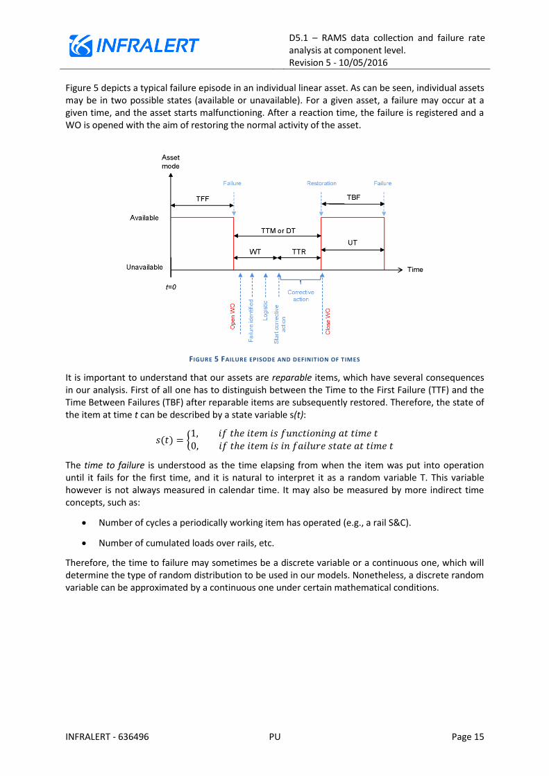
Figure 5 depicts a typical failure episode in an individual linear asset. As can be seen, individual assets may be in two possible states (available or unavailable). For a given asset, a failure may occur at a given time, and the asset starts malfunctioning. After a reaction time, the failure is registered and a WO is opened with the aim of restoring the normal activity of the asset.

FIGURE 5 FAILURE EPISODE AND DEFINITION OF TIMES

It is important to understand that our assets are reparable items, which have several consequences in our analysis. First of all one has to distinguish between the Time to the First Failure (TTF) and the Time Between Failures (TBF) after reparable items are subsequently restored. Therefore, the state of the item at time t can be described by a state variable s(t):

( ) {

The time to failure is understood as the time elapsing from when the item was put into operation until it fails for the first time, and it is natural to interpret it as a random variable T. This variable however is not always measured in calendar time. It may also be measured by more indirect time concepts, such as:

Number of cycles a periodically working item has operated (e.g., a rail S&C).

Number of cumulated loads over rails, etc.

Therefore, the time to failure may sometimes be a discrete variable or a continuous one, which will determine the type of random distribution to be used in our models. Nonetheless, a discrete random variable can be approximated by a continuous one under certain mathematical conditions.



From Figure 5 the following important parameters are defined:

TFF: Time to First Failure, when the item fails for the first time.

TBF: Time Between Failures, which excludes the down time.

TTM or DT: Time To Maintain or Down Time, during which the system (or asset) is not available for operation.

TTM = t(finish corrective action) – t(failure identification)

UT: Up Time or available state, during which the system is in full operation.

WT: Waiting Time, in which the WO has been opened and the system is waiting for a corrective action to be taken.

TTR: Time To Restore, in which the failure has been already identified and the corrective action is taking place.

TTR = t(finish corrective action) – t(start corrective action)

The Relative Restoration Time (RRT) is a ratio defined as RRT(%) = TTR/TTM, and gives an idea of the efficiency of the corrective actions.

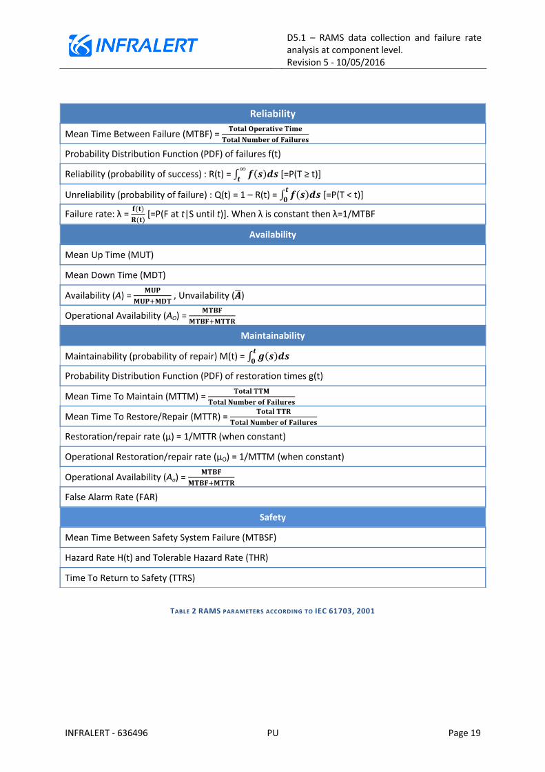
Table 2 shows the definition of the RAMS parameters that will be calculated in this WP according to the standard [13]. Some important remarks are in order:

1) Given a set of failures and times at which these failures occur, MTBF can be evaluated as the average of up times, i.e. cumulative UT, over the total number of failures. This is an important parameter because it is used to estimate the failure rate λ in cases where it is constant as λ=1/MTBF.

Constant failure rates are feasible when failures have a random character. This happens for instance in electronic devices when the malfunctioning components are replaced when they fail. Hence, constant failure rates are a common approximation when only TTFs are considered in the study. As it was pointed out earlier, due to the fact that most items are repairable and because of the system complexity, this is not a good approximation in the case study.

2) The Probability Distribution Function (PDF) of failures f(t) represents the probability that the asset working in time t fails in the interval (t, t+dt). The Reliability R(t) and Unreliability Q(t) are defined in terms of this PDF. The Reliability3 is a function of time t, and is defined as the probability that the duration be greater or equal to t. The Unreliability is the probability that the duration be less than t. By definition Q(t) is the cumulative density function associated to the PDF, i.e., Q(t) = 1- R(t) = F(t), with f(t)=dF(t)/dt.

3) The failure rate λ is formally defined as the (Bayesian) probability of failure at a given time t provided that the system has survived until t. In general this failure rate is a function of time and is assumed to be constant when the rate of occurrence of failures of the components can be considered uniformly random distributed. As already mentioned, in some cases the constant approximation is adopted when items are not repairable, few data is available or the degradation mechanism is unknown. As a matter of fact, the failure rate is sometimes called Force Of Mortality (FOM) to avoid the confusion with this Rate Of Occurrence Of Failures (ROCOF) of a

3 The Reliability function is usually known as survival function in Statistics.



repairable item. The ROCOF is a function of time as repaired items are not as-good-as-new most of the times, and as a consequence their failure rate will not be constant.

4) It is worth commenting at this point that the previous remark is intimately related with the so called Quality Index, an index that takes into account how much a deteriorated infrastructure is, and its impact on safety, speed and riding comfort. Normally, maintenance will not achieve the initial quality of the infrastructure when it was first put into services and for that reason failures will occur more often. Figure 6 shows a typical example of the course of a track quality. When the intervention threshold (desirable driving comfort) is reached, the track is put into its initial state. This period is followed by a growth of the track defect. The initial quality is only recovered in the first few maintenance cycles. After a given amount of cumulated load, the initial quality cannot be achieved again with regular maintenance activities, and after some time it is necessary to proceed with the renewal of the asset.

FIGURE 6 SCHEMATIC COURSE OF TRACK QUALITY [14]

5) The typical behaviour of the failure rate of a component is quite well described by the so called bathtub curve (see Figure 7) after its characteristic shape. The lifetime of an item can be divided into three useful life periods: the burn-in period, the useful-life period and the wear-out period. The failure rate is usually high in the initial phase, due possibly to undiscovered defects (“infant mortality”) of the items which soon show up when the items are active. When the items have survived the infant mortality, the failure rate often stabilizes (useful-life period) at a level where it remains for a certain amount of time until it starts to increase as the items begin to wear out.

FIGURE 7 BATHTUB CURVE



6) Given the complexity of the systems considered, the constant failure rate approximation is not expected to work. As a consequence approaches based on non-parametric or parametric estimators will be more appropriate. Many different types of distributions have been proposed for modelling component failures. Sometimes there are probabilistic arguments based on the physics of failures modes that tend to justify their choices. In other cases, specific models are used solely because of its empirical success in fitting the experimental data. Among these models, the most commonly used (non-parametric) estimators are the Kaplan-Meier and Nelson-Aalen, as well as the (parametric) Exponential, Weibull, Extreme Value, Gamma and Lognormal distributions. One of the tasks that will be developed in this WP is analysing this broad spectrum of models and finding out which of them suit best our data (our infrastructure rail and road systems) and give us the best results.

7) In general Availability A(t) and Maintainability M(t) are functions of time, but take simple expression when both, failure λ and repair µ rates are assumed to be constants. Otherwise, more complex probability distributions for failure f(t) and restorations g(t) need to be considered. Maintainability is the probability that a system be repaired at time t if the corrective action started at t=0.

8) The relationships between the functions F(t) (cumulative density), f(t) (probability density), R(t) (reliability), and λ(t) (failure rate) are presented in Table 1. It can be seen that the reliability function R(t) is uniquely determined by the failure rate function λ(t) for a given type of item.

TABLE 1 RELATIONSHIP BETWEEN FUNCTIONS DEFINING RELIABILITY

F(t) f(t) R(t) λ(t)

F(t) = - ∫ ( )

( ) ( )

( ∫ ( )

)

f(t) =

( )

-

( ) ( ) ( ∫ ( )

)

R(t) = ( ) ∫ ( )

-

( ∫ ( )

)

λ(t) = ( )

( )

( )

∫ ( )

( )

-



TABLE 2 RAMS PARAMETERS ACCORDING TO IEC 61703, 2001

Reliability

Mean Time Between Failure (MTBF) =

Probability Distribution Function (PDF) of failures f(t)

Reliability (probability of success) : R(t) = ∫ ( )

[=P(T ≥ t)]

Unreliability (probability of failure) : Q(t) = 1 – R(t) = ∫ ( )

[=P(T < t)]

Failure rate: λ = ( )

( ) [=P(F at t|S until t)]. When λ is constant then λ=1/MTBF

Availability

Mean Up Time (MUT)

Mean Down Time (MDT)

Availability (A) =

, Unvailability ( ̅)

Operational Availability (AO) =

Maintainability

Maintainability (probability of repair) M(t) = ∫ ( )

Probability Distribution Function (PDF) of restoration times g(t)

Mean Time To Maintain (MTTM) =

Mean Time To Restore/Repair (MTTR) =

Restoration/repair rate (µ) = 1/MTTR (when constant)

Operational Restoration/repair rate (µO) = 1/MTTM (when constant)

Operational Availability (Ao) =

False Alarm Rate (FAR)

Safety

Mean Time Between Safety System Failure (MTBSF)

Hazard Rate H(t) and Tolerable Hazard Rate (THR)

Time To Return to Safety (TTRS)



Explanatory variables Failure status

4.2 ANALYSIS OF RELIABILITY DATA WITH COVARIATES

In many reliability analyses as well as the information on the component’s (or system’s) lifetimes there is also available further information about the component, the system or the environment. Typically there will be information on the design of a given component or the wear the component has suffered. Hence, associated with each lifetime there may be other variables, known as covariates, which give extra information and yield more understanding about the performance of the components or the system.

As pointed out earlier, reliability functions can be modelled using parametric or non-parametric models to account for failure time data. If covariates or explanatory variables (upon which failure time may depend) exist, it becomes of interest to generalize these models to take into account the additional information on the items sampled. This information is interesting for several reasons:

to find significant factors (or variables) which affect lifetime;

to remove nuisance variables which distort the analysis;

to increase comprehension of failure modes; and

to produce a better prediction of the failure rate.

In general, useful covariates explain/predict why some units fail quickly and some units survive a long time. They can be continuous variables like stress, temperature, and pressure; discrete variables like number of loads or number of simultaneous users of a system; or categorical variables like manufacturer, design, and location.

The suitable technique to be used to analyse this type of data is Regression Analysis (supervised learning with continuous responses). In using regression models the aim is to account for the variation in one variable in terms of other variables.

Let us consider the failure time of the assets T>0 (random variable) and suppose that a set of covariates (predictors) is available for each item XT=(X1, X2, …, Xp) giving information about the item and which measures have been taken before time 0. The X’s may contain information on specific characteristics (type of item, physical information, environmental conditions, locations, type of maintenances, etc) in such a way that, aspects of the X’s are supposed to be predictive of subsequent failure times. A typical layout for this data could be the following:

Item # t δ X1 X2 … Xp

1 t1 d1 x11 x12 … x1p 2 t2 d2 x21 x22 … x2p ⁞ ⁞ ⁞ ⁞ ⁞ ⁞ 5 t5 d5 x51 x52 … x5p ⁞ ⁞ ⁞ ⁞ ⁞ ⁞ n tn dn xn1 xn2 … xnp



The first column is an index identifying each item. The remaining columns provide information on the survival time t of the items, the status (whether the item is censured d=0 or uncensored d=1) and further information of interest about the item encoded in the vector of explanatory variables XT=(X1, X2, …, Xp). For instance the explanatory variable X1 may refer to the number of loads and it may vary depending on the item (x4,1 does not have to be equal to x7,1)

4.

X stands for the basic covariates. In general, we may consider models for the failure times that depend on a vector of derived covariates ZT=(Z1, …, Zp) which are obtained as functions of the basic covariates. For instance, interactions (i.e. terms of the type Xi × Xj ) or nonlinearities (i.e. quadratic Xi

2 or cubic Xi

3 terms) could be considered if they are of potential interest. The basic problem consists on determining a relation between the random variable T and the covariate functions Z.

The generalization of the failure model is made by allowing the failure rate to be a function of the time and the covariates X:

( ) ( ).

Two models are generally used to tackle the problem: Proportional Hazard and Accelerate Failure Time models.

Proportional Hazard (PH) Models

The family of PH models assume that the effect of the covariates in the previous failure rate function is multiplicative, i.e. it can encoded in a linear form,

( ) ( ) ( ).

Here ( ) is an arbitrary unspecified function called baseline, ( ) is a functional form which choice may depend on the data being analysed, and . The vector

( ) defines the set of regression parameters to be determined. In the

simplest version (absence of interactions and polynomial terms) the linear term reduces to . The most natural choice for the function ( ) is the one suggested

by [15] and which gives name to his model:

( ) ( ) ( ).

The Cox model can be viewed as a semi-parametric or parametric model, depending whether a functional form for the baseline ( ) is specified or not.

Accelerate Failure Time (AFT) Models

The family of AFT models assume a generalized log-location-scale distribution for T. Let us clarify this; the lifetime T is assumed to have a log-location-scale family of distributions if ln T has a location-scale family of distributions, i.e., it can be written has,

,

where U has a “standardized” distribution centered around 0, with values in ( ).

4 In Machine Learning the value of the feature (name given to covariates) j in the i

th training example is denoted

as ( )

, which may be a clearer notation and may be adopted in the future development of this expert-based

toolkit.



For instance the following cases are often considered,

- if ( ), then - ( )

- if ( ) then - ( )

- if ( ) then ( ) with

.

Then, AFT models assume a distribution for the lifetime of the form,

The interpretation is that the role of Z is to accelerate or decelerate the time to failure.

In this expert-based toolkit regression analysis will be applied to field data in order extract relevant knowledge for RAMS parameters.

4.3 MODEL VALIDATION

As discussed earlier, the use of parametric models implies to select a given probability distribution function. The parameters of such distribution are obtained from the data via maximum likelihood or other statistical techniques. The problem of residual errors estimation comes into play here. Moreover, the model obtained from our analysis to estimate RAMS parameters, whichever it is parametric or non-parametric, needs to be tested in order to have an estimation of our predictive power. For this purpose, and provided enough data is at disposal, resampling techniques [16] [17], such as cross-validation or bootstrap, will be applied. In these techniques the complete data set is divided into two sub-sets. The first set (the training set) is used for model selection and parameter estimation, and the second set (the validation set) is used for model validation and error estimation.

4.4 SOFTWARE / TOOLS

In order to have an idea of how this expert-based toolkit fits in with the rest of the data analytics tasks in INFRALERT, it is worth making some comments about the computing technology that will most probably be used for this particular task.

There is a variety of commercial software available to carry out RAMS analyses. Although commercial software has the advantage of having been previously tested, this type of software packages results most of the times in black-boxes, becoming in loss of control, manoeuvrability and flexibility. One of the goals of this expert-based toolkit is to develop our own algorithms and codes to implement the calculation of RAMS, so they can be efficiently integrated within the rest of the analyses in the project.

It is desirable that our calculations be fast, the access to the Data Farm be easy and that our computational tools be integrated with the rest of the code as much as possible. As a first approach, the use of high level programming languages, such as Python or R, is proposed to implement our models (or calculations) for several reasons. Firstly, they are powerful tools widely used in statistic data analysis. They have become very popular in recent years and as a consequence, numerous packages have been developed which suit our study quite well. Specific survival analysis packages are already available in Python (lifelines, PyRe) and R (survival). Secondly, it is open-source and licence free software, under GNU licence, so cost-less. Thirdly they can be used for Big Data Analytics as they



can implement MapReduce algorithms which may be useful for future applications beyond the scope of this particular project. And finally, R and Python get along well with both relational data bases (for structured data) and non-relational data bases (for highly unstructured data). Both can integrate quite straightforwardly MySQL, MariaDB, Hive, Hadoop, Cassandra, MongoDB among other.



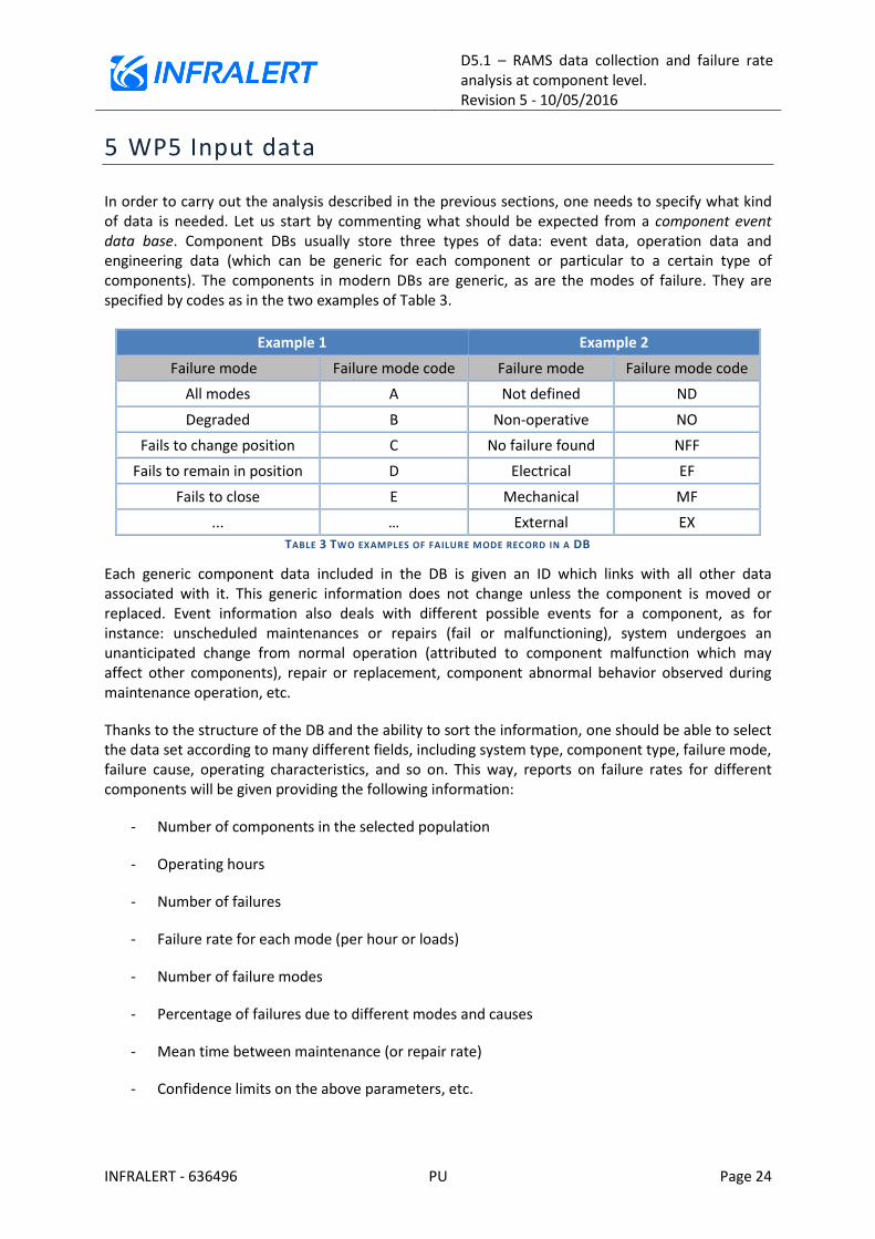
5 WP5 Input data

In order to carry out the analysis described in the previous sections, one needs to specify what kind of data is needed. Let us start by commenting what should be expected from a component event data base. Component DBs usually store three types of data: event data, operation data and engineering data (which can be generic for each component or particular to a certain type of components). The components in modern DBs are generic, as are the modes of failure. They are specified by codes as in the two examples of Table 3.

TABLE 3 TWO EXAMPLES OF FAILURE MODE RECORD IN A DB

Each generic component data included in the DB is given an ID which links with all other data associated with it. This generic information does not change unless the component is moved or replaced. Event information also deals with different possible events for a component, as for instance: unscheduled maintenances or repairs (fail or malfunctioning), system undergoes an unanticipated change from normal operation (attributed to component malfunction which may affect other components), repair or replacement, component abnormal behavior observed during maintenance operation, etc.

Thanks to the structure of the DB and the ability to sort the information, one should be able to select the data set according to many different fields, including system type, component type, failure mode, failure cause, operating characteristics, and so on. This way, reports on failure rates for different components will be given providing the following information:

- Number of components in the selected population

- Operating hours

- Number of failures

- Failure rate for each mode (per hour or loads)

- Number of failure modes

- Percentage of failures due to different modes and causes

- Mean time between maintenance (or repair rate)

- Confidence limits on the above parameters, etc.

Example 1 Example 2

Failure mode Failure mode code Failure mode Failure mode code

All modes A Not defined ND

Degraded B Non-operative NO

Fails to change position C No failure found NFF

Fails to remain in position D Electrical EF

Fails to close E Mechanical MF

... … External EX



The analysis will therefore need historical data of failures and associated WOs for the case studies (road and railway demo cases). The historical maintenance interventions undergone on any of the infrastructure assets will be stored in the Data Farm. Two cases of study and therefore two different sources of data are involved. According to Deliverable D1.2 “Set up of case studies and evaluation framework” [9], work order data will come from SGPav (IP Pavement Management System) and Trafikverket (TRV) and the data structure is described in this deliverable.

The data should at least contain the following information (among other):

Asset ID: which identify the item (asset/system/subsystem)

In service date: restoration date if asset previously failed, or initial service date if censored

Failure date: a recorded date (time) when a failure was detected

Diagnostic: information about the failure if possible

Censure: 1/0 if a failure for the item has/has not been detected yet

Cause of failure: design, electrical, environmental, external, lack of maintenance or incorrect operation, mechanical, no failure found, not defined, etc.

Corrective actions taken: repair/replacement, software restart/update, provisional repair, adjustment, cleaning of obstacles, etc.

This information should be accessible or able to transform from raw data to structured data, so a suitable statistical analysis algorithm can be applied.

According to the documentation already provided in Deliverable D1.2 [9], for the road case the following data files were provided (Table 3 in D1.2):

File Description

v_sgp_xi_seccao Generic information of sections including values of parameters from last inspection

v_sgp_xi_no Node points that are used to define sections

t_sgp_seccao_campanhap Metadata of the measurements done for each section, made with the laser profiler

t_sgp_seccao_campanhap_obs Values of measurements for each 10 meter made with the laser RST profiler

t_sgp_seccao_campanhap_eve Events (collected visually) during inspection

t_sgp_seccao_campanhap_iq Aggregated calculated values, including Quality index, for aggregations above or equal to 100m

v_sgp_xi_img Right of way images collected with RST profiler

t_sgp_seccao_scrim Metadata of the measurements done for each section, with the SCRIM (for SKID resistance)

t_sgp_seccao_scrim_obs Values of measurements for each 10 meter made with the SCRIM

v_sgp_xi_historico Pavement interventions inventory

t_sgp_seccao_obra Maintenance and rehabilitation pavement interventions and its costs



File Description

Rede_Infralert_20150630_CODSEC_SEC_ID Shape files with geographical information of the road sections used in the case study

TABLE 4 FILES PROVIDED FOR TH E ROAD DEMO CASE

In principle the needed information can be retrieved from these tables, specifically from t_sgp_seccao_campanhap_eve, v_sgp_xi_historico and t_sgp_seccao_obra.

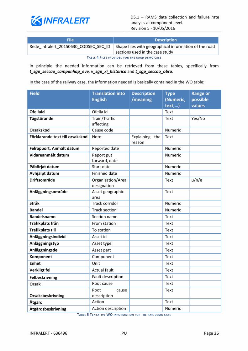
In the case of the railway case, the information needed is basically contained in the WO table:

Field Translation into English

Description /meaning

Type (Numeric, text,…)

Range or possible values

OfeliaId Ofelia id Text

Tågstörande Train/Traffic affecting

Text Yes/No

Orsakskod Cause code Numeric

Förklarande text till orsakskod Note Explaining the reason

Text

Felrapport, Anmält datum Reported date Numeric

Vidareanmält datum Report put forward, date

Numeric

Påbörjat datum Start date Numeric

Avhjälpt datum Finished date Numeric

Driftsområde Organization/Area designation

Text u/n/e

Anläggningsområde Asset geographic area

Text

Stråk Track corridor Numeric

Bandel Track section Numeric

Bandelsnamn Section name Text

Trafikplats från From station Text

Trafikplats till To station Text

Anläggningsindivid Asset id Text

Anläggningstyp Asset type Text

Anläggningsdel Asset part Text

Komponent Component Text

Enhet Unit Text

Verkligt fel Actual fault Text

Felbeskrivning Fault description Text

Orsak Root cause Text

Orsaksbeskrivning Root cause description

Text

Åtgärd Action Text

Åtgärdsbeskrivning Action description Numeric

TABLE 5 TENTATIVE WO INFORMATION FOR THE RAIL DEMO CASE



6 WP5 Outputs

RAMS and LCC analyses will follow a stochastic approach whose objective is to obtain failure information (in form of distributions) of the entire system based on the failure distributions of its components. Although this will be described in more detail in forthcoming deliverables, it is worth commenting here the expected type of outputs.

In the previous sections, the methodology to be followed to calculate RAMS parameters at component level has been described. These parameters will contain information on failure and repair times in the form of statistical estimates. From RAMS at component level one can access system RAMS by different approaches (reliability block diagrams, fault tree, Markov chain method, flow networks, Petri nets or Monte Carlo next event simulation, among others). Probably the most flexible of all these approaches is Monte Carlo next event simulation, because it can be used to analyse almost any type of system. More information will be given in Deliverable D6.1.

From a model for the system as a whole, and the previous knowledge of RAMS parameters at component level, Monte Carlo next event simulation is carried out by simulating typical lifetime scenarios for the system under study. Random events (i.e., events associated to item failures) are generated which together with scheduled events (e.g., preventive maintenance actions) and conditional events (i.e., initiated by the occurrence of other events) are included to create a scenario as close as possible to reality.

The simulation plays the role of a “real experiment”, from which rich probabilistic information from the system can be accessed. These are for instance, estimates of performance measures of interest as mean values (MTBF, MTTF, MRL), confidence limits, higher order moments, p-values, statistical tests (ANOVA) or underlying probability distribution functions (distributions of system failures).

The input of the simulation is a model for the system and the RAMS at component levels. The outputs of the simulation are probabilistic estimates for RAMS parameters at system level, and as such, they are subject to uncertainty. These outputs can be eventually used in stochastic optimization (optimization under uncertainties) to be carried out in the Smart decision support framework. Moreover, thanks to the simulation, and regression analysis, the most prone failure modes to occur will be revealed. This information will be of great importance because it can be used to predict faults and condition evolving in specific asset components, as well as to improve the predicting capability of asset’s alerts and the efficiency of the asset management system.



7 Conclusions

This deliverable has presented the relevant information needed by the RAMS&LCC toolkit developed in WP5 to calculate RAMS parameters. For this purpose, the deliverable has described the methodology that will be followed, the set of parameters to be calculated, the input data needed to calculate them and the results or output data that will be obtained as a product.

The information presented herein is a framework based on current basic knowledge, and as such, it may be subject to improvements, revisions or modifications during the progress of this WP.



8 Glossary of terms

Asset The physical transportation infrastructure (e.g. travel way, structures, etc.); more generally can include the full range of resources capable of producing value-added for an agency (e.g. human resources, equipment, materials, financial capacity, real state, corporate information, etc.).

Availability The percentage of time that a system is able to perform its required functions at a stated instant of time or over a stated period of time. The faster the system can be repaired after a failure, the greater the availability (EN50126, 1999).

Censoring Censoring is present when some information about a subject or item’s event time is available, but the exact event time is unknown, so it restrict the ability to observe failure time exactly.

Covariate Variable X that is possibly predictive of an outcome or response Y through the relation Y=f(X)+ε, where ε is an error term. In statistics is also known as independent variable, predictor, regressor, explanatory o feature (in machine learning).

Failure Departure of a component’s functionality targets from specification (Smith, 2005). Termination of the ability of an entity to perform a required function under specified conditions (Villemeur, 1992).

Linear asset An asset not specific to a single location representing a network. For example, oil and gas pipe lines, roads, highways, rail tracks and utility lines (water, sewage and power [8] transmission). They can cross over with other networks and hold many non-linear assets (traffic control systems, stations, power generating stations).

Maintainability The ability of an item, under stated conditions of use, to be retained in, or restored to, a state in which it can perform it required functions. The probability that a failed item will be restored to operational effectiveness (Smith, 2011; EN50126, 1999).

Regression Statistical method that attempts to determine the strength of the relationship between one dependent variable (usually denoted Y) and a series of other changing variables (known as independent variables or covariates).

Reliability The probability that an item will perform a required function, under stated conditions, for a stated period of time (Smith, 2011; EN50126, 1999).

Repairable item Items that can be repaired after a failure has occurred.

Safety Freedom from those conditions that can cause an unacceptable damage risk such as death, injury, occupational illness, or damage to or loss of equipment or property (EN50126, 1999).



9 References

[1] Norwegian University of Science and Technology, «Reliability Data Sources - ROSS - NTNU,» Available at: http://www.ntnu.edu/ross/info/data [Accessed 5 Apr. 2016], Trondheim (Norway), 2016.

[2] J. van den Breemer, «RAMS and LCC in the design process of infrastructural construction projects : an implementation case. Civil Engineering and Management MSc (60026),» Available at: http://essay.utwente.nl/, University of Twente, The Netherlands, 2009.

[3] S. Al-Jibouri y G. Ogink, «Proposed model for integrating RAMS method in the design process in construction.,» Architectural Engineering and Design Management, 5(4), 179–92, 2009.

[4] W. R. Blischke y D. N. P. Murthy, «. Reliability: Modeling, Prediction, and Optimization (Wiley Series in Probability and Statistics),» John Wiley & Sons, New Jersey, 2000.

[5] W. R. Blischke y M. D. N. Prabhakar, «Case Studies in Reliability and Maintenance (Wiley Series in Probability and Statistics),» John Wiley & Sons, New Jersey, 2003.

[6] D. N. P. Murthy, M. Xie y R. J. Murthy, «Weibull Models (Wiley series in probability and statistics),» John Wiley & Sons, New Jersey, 2004.

[7] D. J. Smith, «Reliability, Maintainability and Risk 8th Edition: Practical Methods for Engineers including Reliability Centred Maintenance and Safety-Related Systems,» Butterworth-Heinemann, Oxford, 2011.

[8] European Commettee for Electronical Standardization, «UNE-EN 50126-1:2010. Railway applications - The specification and demonstration of Reliability, Availability, Maintainability and Safety (RAMS). Part 1: Basic requirements and generic process. British Standards (BSI).,» Brussels, 2010.

[9] INFRALERT consortium, «Deliverable D1.2 Definition of case studies and evaluation framework,» INFRALERT project, H2020, 2015.

[10] E. T. Lee and J. Wang, Statistical methods for survival data analysis, 2nd ed., New Jersey: John Wiley & Sons, 2003.

[11] J. P. Klein y M. L. Moeschberger, «Survival analysis: Techniques for censored and truncated data,» Springer-Verlag, New York, 2003.

[12] J. F. Lawless, «Statistical Models and Methods for Lifetime Data.,» Wiley-Interscience, New Jersey, 2002.

[13] International Electrotechnical Commission (IEC), «Mathematical expressions for reliability, availability, maintainability and maintenance support terms. n.61703,» International Electrotechnical Commission, Geneva, 2001.

[14] B. Lichtberger, «Track Compendium: Formation, Permanent Way, Maintenance, Economics. Eurailpress, Hamburg.,» 2005.



[15] D. R. Cox, «Regression models and life-tables.,» Journal of the Royal Statistical Society. Series B (Methodological), 34, 187. Retrieved from http://www.jstor.org/stable/2985181, London, 1972.

[16] B. Efron y R. Tibshirani, «An Introduction to the Bootstrap,» Chapman and Hall/CRC, London, 1994.

[17] P. I. Good, «Introduction to Statistics Through Resampling Methods and R (2nd Ed.).,» Wiley, New Jersey, 2013.

RAMS data collection and failure rate analysis at...

Documents

Transcript of RAMS data collection and failure rate analysis at...