R&D White Paper - downloads.bbc.co.uk

R&D White Paper

WHP 080

April 2004

Modelling impulsive interference in DVB-T: statistical analysis, test waveforms & receiver performance

J. Lago-Fernández and J. Salter

Research & Development BRITISH BROADCASTING CORPORATION

© BBC 2004. All rights reserved.

BBC Research & Development White Paper WHP 080

Modelling Impulsive Interference in DVB-T:

Statistical Analysis, Test Waveforms and Receiver Performance

José Lago-Fernández, John Salter

Abstract

Impulsive interference is an elusive phenomenon which cast a shadow on the initial success of Digital Terrestrial Television in the UK at the time of launch of ITV Digital. The unavailability of suitable test methods for impulsive noise has also hindered the search for new measures to counter its effect. Until now, gated Gaussian noise had been widely recognised as the only calibrated tool available to measure impulsive interference performance. From October 2001 to October 2002 a working group within the DTG led by BBC R&D carried out a series of theoretical and practical studies to devise a representative set of test waveforms for impulsive interference. A statistical parametric model for impulsive interference based on randomly pulsed bursts of Gaussian noise was fitted to a large set of captures of real impulsive noise. This model was extensively used in laboratory measurements and its applicability was validated. The result of all this work was the proposal of a group of new ‘gated-squared’ Gaussian noise tests. Some recommendations for test methods and measurement equipment were also made. As a by-product of this measurement campaign came the realisation that the impulsive noise performance of a DTT receiver equipped with no specific countermeasures can be determined from the effective duration of the burst of noise.

A shortened version of this white paper is to be published in the EBU Technical Review.

Key words: Ignition noise, EMC, statistics

© BBC 2004. All rights reserved.





Contents

1 Introduction............................................................................................................................. 1 2 What is impulsive interference?.............................................................................................. 2 3 Capturing impulsive interference............................................................................................ 3

4 The statistics of impulsive interference................................................................................... 4 5 Preliminary recommendation for impulsive noise tests........................................................... 7 6 Experimental results................................................................................................................ 8

6.1 Capture waveforms + SMIQ results................................................................................... 10 6.2 Preliminary test waveforms results.................................................................................... 13

7 DTG impulsive noise test waveforms.................................................................................... 19

8 Conclusions........................................................................................................................... 20 Acknowledgements......................................................................................................................... 20 Glossary .......................................................................................................................................... 21

References....................................................................................................................................... 22 A Sample captures and histograms for impulsive interference.................................................. 23 B Additional DVB-T II performance plots for capture waveforms + SMIQ............................. 41

© BBC 2004. All rights reserved. Except as provided below, no part of this document may be reproduced in any material form (including photocopying or storing it in any medium by electronic means) without the prior written permission of BBC Research & Development except in accordance with the provisions of the (UK) Copyright, Designs and Patents Act 1988.

The BBC grants permission to individuals and organisations to make copies of the entire document (including this copyright notice) for their own internal use. No copies of this document may be published, distributed or made available to third parties whether by paper, electronic or other means without the BBC's prior written permission. Where necessary, third parties should be directed to the relevant page on BBC's website at http://www.bbc.co.uk/rd/pubs/whp for a copy of this document.

White Papers are distributed freely on request.

Authorisation of the Chief Scientist is required for publication.

1





1 Introduction

Impulsive interference (II) has been an elusive phenomenon casting a shadow on the initial launch of Digital Terrestrial Television (DTT) in the UK in 1998. The lack of a suitable time-interleaving scheme in the DVB-T specification makes the system rather sensitive to sources of interference of impulsive nature. Strategies for improving the performance of DTT in the presence of impulsive noise have met with varying success. One reason for this is the unavailability of a DTT model for II that can be used by set-top box and demodulator chip manufacturers to develop new II countermeasures.

In October 2001 a working group within the Digital Television Group (DTG) led by BBC R&D and formed by Sony, Philips, Rohde & Schwarz, Zarlink and ST Microelectronics was set up. Other invited parties included Roke Manor Research and the Radiocommunications Agency. The aims were to propose a set of test waveforms and methods which could be used to faithfully represent the effect II has on DTT. At that time, this task did not seem to be too complex. However, just like a previous DTG Interference Working Group, the present group soon discovered this subject is very complex.

This white paper reports on the work done by the BBC as a member of the DTG II working group from October 2001 to October 2002. Basically, our contribution to the group consisted of two main areas of work:

• Capture and statistical analysis of real impulsive interference so as to come up with a simulation model for II

• Campaign of laboratory measurements to validate and simplify the proposed model. These measurements were also used as an assessment of the key parameters determining the performance of DTT when affected by II

In Section 2 we give a brief description of what impulsive interference is and how it has been modelled in the literature. The use of a previously designed system to capture impulsive noise in different environments is the subject of Section 3. The statistical model proposed within the DTG II working group is presented in Section 4 together with the statistical analysis performed on all captured data. A preliminary suite of test waveforms is introduced in Section 5, whilst Section 6 presents a summary of the laboratory results obtained using these waveforms in different setups. The test waveforms finally agreed within the working group are presented in Section 7. This same section describes test methods and suggests the measurement equipment that can be utilised to carry out II tests in a DTT system. Finally, a brief summary and conclusions are presented in Section 8. A glossary, a list of references and two appendices are included at the end of the document.

2

2 What is impulsive interference?

A variety of naturally occurring and man-made phenomena exhibit impulsive behaviour. Impulsive noise is usually described in the literature as a process characterised by bursts of one or more short pulses whose amplitude, duration and time of occurrence are random [1]. The inter arrival time of these pulses is generally assumed to be greater than the time constants of the measuring system. This does not introduce any restrictions and simply means that individual pulses can be resolved by the system.

There are many potential sources of impulsive interference in a domestic DTT installation:

• House appliances (washing machine, dish washer, food mixer, iron, oven, kettle, electric razor, drill, microwave oven, etc.)

• Central heating thermostats

• Light switches (fluorescent, incandescent, etc.)

• Ignition systems (traffic, lawn mower, etc)

The first three can affect the DTT receiver through ingress into the downlead and/or flylead. The use of properly screened cables and mains outlets is of paramount importance here. Also, the use of a balun antenna reduces the coupling considerably. Ignition interference is received by the rooftop antenna and cannot be so easily eliminated.

Impulsive noise models for systems operating at low frequencies have been proposed by the ITU [1]. These models are based on measurements of median levels of interfering noise. However, for higher frequencies as used in DTT and other digital transmission systems, high peak levels of interference may adversely affect reception even though the measured median level of the interferer does not rise above the background noise. This is why a fresh approach was needed to characterise impulsive interference in the UHF band.

Mathematically, impulsive interference is usually modelled as a train of pulses which can be expressed as [2, 3]

� −=i

iwi tPAtni

)()( τ (1)

where the amplitude Ai, duration Wi and arrival time τi of each pulse is a random variable whose distribution is a priori unknown. The parametric model above is fully defined when we establish the statistical distribution of the three parameters characterising each pulse.

In [2] the arrival times are modelled using a gamma distribution (which includes the exponential distribution and periodic function as particular cases). The RF bandwidth of impulsive interference is typically much greater than that of the measuring system [1, 4]. The shape of the pulses is therefore given by the impulse response of the actual receiving or measuring system. In [2] an exponentially decaying unit step is used as a typical pulse. When the measuring system is operating at an intermediate frequency fI, the impulse response further modulates a carrier of frequency fI. The amplitude of the pulses can be modelled using either a lognormal distribution or a power-Rayleigh distribution. The choice of statistical distribution for each parameter made in [2] seems rather arbitrary since it is based on models available in the literature which are usually either too specific or excessively theoretical. The applicability of these results to DTT is thus rather limited.

In [5] the model in (1) is used to characterise impulsive interference in the UHF bands using a 10 MHz measurement bandwidth. In this study no suitable probability distribution could be

3

reliably fitted to the measured pulse amplitudes and time spacing between pulses1. The pulse duration seemed to be gamma-distributed and, in outdoor environments, it was apparently correlated with the amplitude of the pulse. This should come as no surprise since the power spectrum of impulsive interference is much wider than that of the measurement system and can be assumed to be constant across a UHF channel [4]. Therefore, both the observed amplitude and pulse duration are closely related to the measurement bandwidth employed.

A similar statistical analysis in the VHF/UHF bands using a 10 kHz measurement bandwidth and a time resolution of 50 µs was presented in [6]. In this case only vehicle ignition noise was considered. The amplitude of the pulses2 was modelled using a lognormal distribution, whereas the time spacing between consecutive pulses was observed to be uniformly distributed between 5 and 15 ms. The measured pulse duration was about 150 µs. This parameter is sensitive to the measurement bandwidth used in the analysis and probably would have been much lower had a greater bandwidth been used.

Another statistical model mentioned in [1] is the so-called Noise Amplitude Distribution (NAD), which gives the number of pulses per second which exceed a given energy threshold. Allegedly, this is the most appropriate noise descriptor for single-carrier digital systems. For multi-carrier systems, as we will see in Section 6, it is not the rate at which noise energy varies within an OFDM symbol but the total amount of energy that determines the performance of the system3. The NAD seems of little use in this case.

3 Capturing impulsive interference

To gather a sufficiently large set of captured II data we used a capture system which takes 200-ms snapshots of an 8-MHz clean DTT channel filtered and down converted to 2nd IF (central frequency 4.57 MHz and 7.61 MHz bandwidth). The captured waveforms span several hundred OFDM symbols and in most cases are long enough to hold complete impulsive events. Data is sampled at 40 MHz using a 12-bit ADC. The time resolution of the captures is 25 ns.

A similar capture system is proposed in [1]. The measurement bandwidth is slightly greater (10 MHz) and the sampling frequency is lower (25 MHz).

More than two hundred captures were taken at several households and also at locations where traffic interference could be detected. A 200-ms capture contains the impulsive noise waveform responsible for triggering the capture system. This waveform may consist of just one impulsive event or several impulsive events. The definition of event is somewhat subjective and is related to the behaviour of a typical DTT receiver. A new impulsive event starts when the time elapsed between this event and the previous one is greater than the “recovery time” of the receiver. This recovery time represents the time it takes the receiver to completely reacquire lock after having lost synchronisation because of a previous error event.

Appendix A shows sample waveforms for each of the categories the set of captures has been divided into. From a purely theoretical point of view, the amount of data we need to capture for each category should depend on some sort of a priori knowledge about the statistical distribution of the parameters were are trying to estimate. In most cases not even a rough estimate of this information is available and therefore we tried to capture as many impulsive events as possible.

__________________________________________________________________________________________ 1 Which evidences the difficulty in fitting a statistical model to impulsive interference. 2 Measured above a certain threshold carefully chosen above the background noise level. 3 When no special II counter measures are used.

4

4 The statistics of impulsive interference

A sentence that summarises the chaotic nature of impulsive interference is “no two impulsive events are the same” . Trying to characterise it statistically using a complex model may thus sound too ambitious. Instead, it seems more plausible to use a simple model to characterise II as seen by a DTT receiver at IF, that is, to model II once it has been downconverted and band limited to 8 MHz. This model could be used by chip manufacturers in their research for new algorithms to counter II.

If it were the impact of II on the receiver front end that we are interested in, as it is the case for tuner and antenna manufacturers, another approach would be to replicate the actual impulses occurring at the aerial input. Philips has contributed to the DTG II working group with some work on this area. The main drawback of this method seems to be the accurate calibration of the equipment used to generate the fast edges4. Further work would be needed to assess the applicability of this approach.

As described in Appendix A, all captured data was classified and catalogued as belonging to one of the following categories:

• Central heating types 1, 2 and 3

• Cooker ignition

• Dishwasher

• Light switches being thrown off

• Fluorescent and incandescent light switches being thrown on

• Traffic interference types 1, 2 and 3

Some other capture groups such as drill or food mixer were discarded because their chaotic nature prevented any further analysis.

To each of these groups of captures we tried to fit the statistical model shown in Figure 1. The model is similar to that proposed in (1). An impulsive event is made of one or more bursts. Each of these bursts contains a number of pulses. The pulse amplitude AP is assumed constant. In reality the amplitude of the pulses varies largely within the same capture but in an apparently chaotic and unpredictable way (see Appendix A). PS is the spacing between pulses within the same burst and equals the distance between arrival times in (1). PD and BD denote the duration of a pulse and a burst, respectively. BS represents the spacing between consecutive bursts. Appendix A details how this model is fitted to the II data set.

Am

plitu

de

Time

Burst n Burst n+1BS

PD

PS

BD

AP

Figure 1: Parametric model for impulsive noise used in the capture data fit.

__________________________________________________________________________________________ 4 It is very difficult to relate a voltage transition at the antenna input to the total energy in any UHF channel because small changes in the rise time slope have a large effect in the energy of the interference.

5

Upon visual inspection of the histograms shown in Appendix A, the difficulty in adjusting a statistical distribution to each of the six parameters AP, PD, PS, BD, BS and event duration ED becomes evident (Appendix A explains the nomenclature used). In view of this, and after several brainstorming sessions within the DTG II working group, the following conclusions and compromises were reached:

• Pulse amplitude is to be held constant within an impulsive event. This stems from the fact that it proved almost impossible to glean any useful information from the different pulse amplitude distributions (APD). The actual amplitude level of the simulated interferer can be varied to change its total power.

• Pulse duration is assumed constant and is fixed at 250 ns. As we mentioned earlier, the elementary pulses within a burst are shaped by the impulse response of the tuner. This response spreads the energy of the incoming short impulses over about 200 to 350 ns. The actual figure depends on how narrow the incoming impulses are. If we accept the rising times of the edges at the input to the aerial to be negligible when compared with the duration of the tuner’s impulse response, then fixing PD at 250 ns does not imply a loss of generality in our model. Besides, in our statistical analysis PD is estimated by taking into account both the rising and falling edges of the tuner’s impulse response. In practice, this tends to overestimate the basic pulse duration. As a side note, the mean pulse duration measured in [5] is 230 ns.

• PS follows a uniform distribution. Again no statistical distribution could be fitted to the PSD histograms and therefore uniform distributions with suitably chosen lower and upper limits are used. In [5] the pulse spacing was deemed to vary between 37 and 54 µs. We found a much greater variation in our results.

• A burst is not allowed to last more than a useful OFDM symbol (224 µµµµs for the UK). Bursts longer than this can be treated as Gaussian noise as far as DVB-T is concerned. It also seemed more appropriate to express the duration of a burst as a number of pulses per burst rather than a time duration.

• BS is fixed at 10 ms. Closely spaced bursts fill in the whole OFDM symbol and are usually too destructive for DVB-T. It was agreed within the working group to use a fixed burst spacing so that by the time a new impulsive burst hits the receiver the effect of previous bursts has long died away. This burst spacing is also consistent with the repetition period of engine ignition interference [6].

• The observation period determines the duration of the impulsive event. A new burst is generated every 10 ms and this is repeated until the observation period chosen for the measurements elapses5. Typically a 1-minute observation period is used.

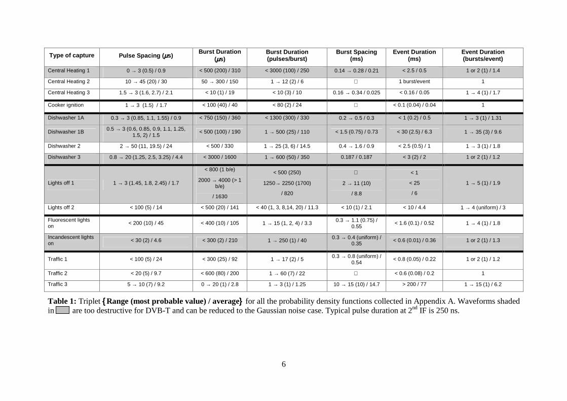
For each type of capture Table 1 summarises the range as lower limit to upper limit (→) or just upper (<) or lower limits (>), the approximate value at which histograms peak, and the mean value for histograms PSD, BDD, BSD and EDD (these terms refer to probability distributions of PS, BD, BS and ED, respectively). Interference types shaded in grey have the same effect as Gaussian noise and are thus not further considered.

Figures in Table 1 are the result of several discussions within the DTG II working group. Sometimes they are just rough guesses or rather loose bounds on the actual values. This simplification was found necessary in order to rationalise the vast amount of data available.

__________________________________________________________________________________________ 5 Note that we are mixing the fit of capture data to our statistical model with the actual use of this model to simulate impulsive interference in the laboratory. Both are closely related and the latter conditions any subjective choice we might have to make in the model fitting process.

6

Type of capture Pulse Spacing (µµµµs) Burst Duration

(µµµµs) Burst Duration (pulses/burst)

Burst Spacing (ms)

Event Duration (ms)

Event Duration (bursts/event)

Central Heating 1 0 → 3 (0.5) / 0.9 < 500 (200) / 310 < 3000 (100) / 250 0.14 → 0.28 / 0.21 < 2.5 / 0.5 1 or 2 (1) / 1.4

Central Heating 2 10 → 45 (20) / 30 50 → 300 / 150 1 → 12 (2) / 6 1 burst/event 1

Central Heating 3 1.5 → 3 (1.6, 2.7) / 2.1 < 10 (1) / 19 < 10 (3) / 10 0.16 → 0.34 / 0.025 < 0.16 / 0.05 1 → 4 (1) / 1.7

Cooker ignition 1 → 3 (1.5) / 1.7 < 100 (40) / 40 < 80 (2) / 24 < 0.1 (0.04) / 0.04 1

Dishwasher 1A 0.3 → 3 (0.85, 1.1, 1.55) / 0.9 < 750 (150) / 360 < 1300 (300) / 330 0.2 → 0.5 / 0.3 < 1 (0.2) / 0.5 1 → 3 (1) / 1.31

Dishwasher 1B 0.5 → 3 (0.6, 0.85, 0.9, 1.1, 1.25, 1.5, 2) / 1.5

< 500 (100) / 190 1 → 500 (25) / 110 < 1.5 (0.75) / 0.73 < 30 (2.5) / 6.3 1 → 35 (3) / 9.6

Dishwasher 2 2 → 50 (11, 19.5) / 24 < 500 / 330 1 → 25 (3, 6) / 14.5 0.4 → 1.6 / 0.9 < 2.5 (0.5) / 1 1 → 3 (1) / 1.8

Dishwasher 3 0.8 → 20 (1.25, 2.5, 3.25) / 4.4 < 3000 / 1600 1 → 600 (50) / 350 0.187 / 0.187 < 3 (2) / 2 1 or 2 (1) / 1.2

Lights off 1 1 → 3 (1.45, 1.8, 2.45) / 1.7

< 800 (1 b/e)

2000 → 4000 (> 1 b/e)

/ 1630

< 500 (250)

1250→ 2250 (1700)

/ 820

2 → 11 (10)

/ 8.8

< 1

< 25

/ 6

1 → 5 (1) / 1.9

Lights off 2 < 100 (5) / 14 < 500 (20) / 141 < 40 (1, 3, 8,14, 20) / 11.3 < 10 (1) / 2.1 < 10 / 4.4 1 → 4 (uniform) / 3

Fluorescent lights on < 200 (10) / 45 < 400 (10) / 105 1 → 15 (1, 2, 4) / 3.3 0.3 → 1.1 (0.75) /

0.55 < 1.6 (0.1) / 0.52 1 → 4 (1) / 1.8

Incandescent lights on < 30 (2) / 4.6 < 300 (2) / 210 1 → 250 (1) / 40 0.3 → 0.4 (uniform) /

0.35 < 0.6 (0.01) / 0.36 1 or 2 (1) / 1.3

Traffic 1 < 100 (5) / 24 < 300 (25) / 92 1 → 17 (2) / 5 0.3 → 0.8 (uniform) / 0.54

< 0.8 (0.05) / 0.22 1 or 2 (1) / 1.2

Traffic 2 < 20 (5) / 9.7 < 600 (80) / 200 1 → 60 (7) / 22 < 0.6 (0.08) / 0.2 1

Traffic 3 5 → 10 (7) / 9.2 0 → 20 (1) / 2.8 1 → 3 (1) / 1.25 10 → 15 (10) / 14.7 > 200 / 77 1 → 15 (1) / 6.2

Table 1: Triplet {{{{Range (most probable value) / average}}}} for all the probability density functions collected in Appendix A. Waveforms shaded in are too destructive for DVB-T and can be reduced to the Gaussian noise case. Typical pulse duration at 2nd IF is 250 ns.

7

5 Preliminary recommendation for impulsive noise tests

Once the bulk of captured data has been analysed and the table on page 6 has been compiled, we are in a position to propose a preliminary set of test waveforms conforming to the template shown in Figure 1. The basic requirements for these test waveforms as agreed within the II working group are:

• They must be representative of actual interference. Albeit somewhat tailored to the peculiarities of the DVB-T system, this has been borne in mind when doing the statistical analysis and subsequent data fit

• They must be easily reproducible, repeatable and should yield the same results regardless of who uses them

• Test and measurement equipment must be readily available to the user

Table 2 and Table 3 gather the nine test waveforms initially proposed within the DTG II working group. These waveforms were used in many DVB-T II performance tests carried out in the laboratory. A summary of these results is presented Section 6. A more complete compilation of plots and results can be found in Appendix B. The main purpose of these tests was to further reduce the number of waveforms needed to simulate II in a DTT system.

The pulse spacing in Table 2 is uniformly distributed and is expressed as a mid-range value plus or minus a “dither” factor. Burst duration is expressed in number of pulses per burst. From the bounds on PS we can work out the minimum and maximum burst durations in µs. Contrary to the burst duration, which includes the time spacing between pulses, the effective burst duration τE is defined as the number of pulses per burst times the pulse duration. That is, τE represents the total amount of time the interference is ‘on’ . Captures traffic 3A and 3B in Table 2 correspond to the two types of captures identified in Section A.14.

Table 3 complements the tests in Table 2 with two gated Gaussian noise tests. This type of tests has been widely used in the past [4]. Test GN1 accounts for the class of noise-like impulsive interferers with 100-µs bursts spaced by just 1 ms. Test GN2 is a downscaled version of the specification for impulsive interference made by Canal +6.

The Canal + proposal was originally made for DVB-T modes using 8K carriers. The chosen burst duration was 3 µs. The burst repetition rate was given by

1

2

11

001.1−

��

��

� +=GT

RS

where ( )GTT US /11+= , being 1/G the guard interval fraction. For instance, in the UK G =

32, TU = 224 µs and 1/R = 234.38 µs. This short repetition period means that each 2K OFDM symbol is effectively corrupted by a burst of Gaussian noise. For the sake of completeness we have tailored the Canal + test to UK DTT system. More precisely, the burst duration is divided by 4 to account for the difference in number of carriers whilst the burst spacing is increased from 1/R to 10 ms for consistency with the other tests.

__________________________________________________________________________________________ 6 Contribution to the DTG II working group from Philips.

8

Noise type

Type of capture accounted for

Pulse spacing

(µµµµs)

Burst duration (pulses per

burst)

Minimum and maximum burst

duration (µµµµs)

Effective burst

duration ττττE

N1 CH type 2 25 ± 10 6 75.25 → 175.25 1.5 µs

N2 CH type 3 2 ± 0.5 2 1.75 → 2.75 500 ns

N3 Cooker ignition 1.5 ± 0.5 20 19.25 → 38.25 5 µs

N4 Dishwasher type 2 & Light s off type 2 12.5 ± 2.5 10 90.25 → 135.25 2.5 µs

N5 Fluorescent light s on 25 ± 20 2 5.25 → 45.25 500 ns

N6 Traffic 3A 7.5 ± 2.5 2 5.25 → 10.25 500 ns

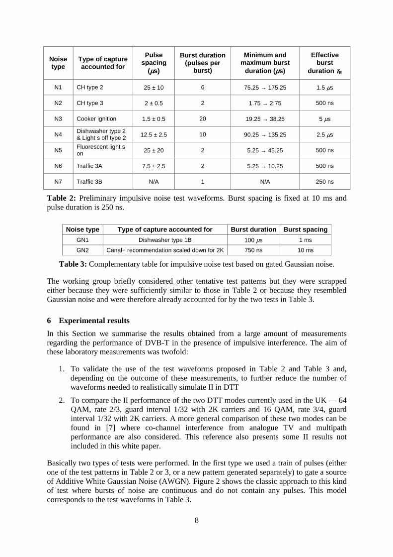
N7 Traffic 3B N/A 1 N/A 250 ns

Table 2: Preliminary impulsive noise test waveforms. Burst spacing is fixed at 10 ms and pulse duration is 250 ns.

Noise type Type of capture accounted for Burst duration Burst spacing

GN1 Dishwasher type 1B 100 µs 1 ms

GN2 Canal+ recommendation scaled down for 2K 750 ns 10 ms

Table 3: Complementary table for impulsive noise test based on gated Gaussian noise.

The working group briefly considered other tentative test patterns but they were scrapped either because they were sufficiently similar to those in Table 2 or because they resembled Gaussian noise and were therefore already accounted for by the two tests in Table 3.

6 Experimental results

In this Section we summarise the results obtained from a large amount of measurements regarding the performance of DVB-T in the presence of impulsive interference. The aim of these laboratory measurements was twofold:

1. To validate the use of the test waveforms proposed in Table 2 and Table 3 and, depending on the outcome of these measurements, to further reduce the number of waveforms needed to realistically simulate II in DTT

2. To compare the II performance of the two DTT modes currently used in the UK — 64 QAM, rate 2/3, guard interval 1/32 with 2K carriers and 16 QAM, rate 3/4, guard interval 1/32 with 2K carriers. A more general comparison of these two modes can be found in [7] where co-channel interference from analogue TV and multipath performance are also considered. This reference also presents some II results not included in this white paper.

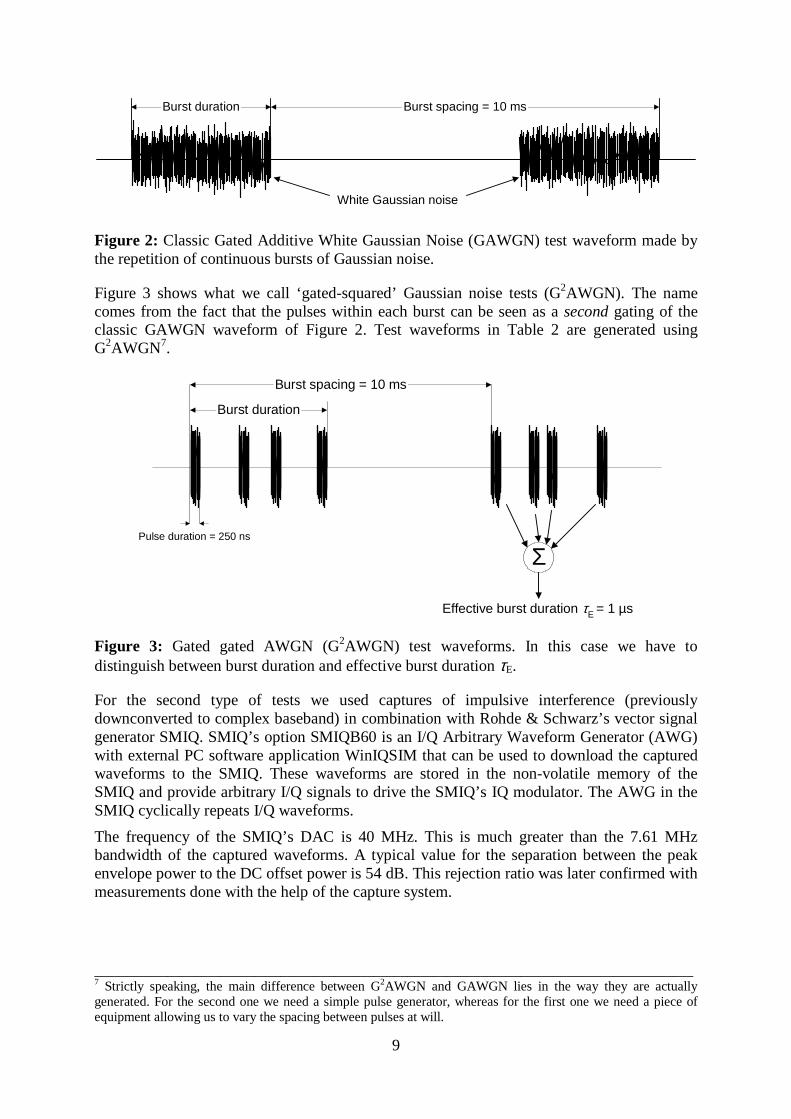
Basically two types of tests were performed. In the first type we used a train of pulses (either one of the test patterns in Table 2 or 3, or a new pattern generated separately) to gate a source of Additive White Gaussian Noise (AWGN). Figure 2 shows the classic approach to this kind of test where bursts of noise are continuous and do not contain any pulses. This model corresponds to the test waveforms in Table 3.

9

Burst duration Burst spacing = 10 ms

White Gaussian noise

Figure 2: Classic Gated Additive White Gaussian Noise (GAWGN) test waveform made by the repetition of continuous bursts of Gaussian noise.

Figure 3 shows what we call ‘gated-squared’ Gaussian noise tests (G2AWGN). The name comes from the fact that the pulses within each burst can be seen as a second gating of the classic GAWGN waveform of Figure 2. Test waveforms in Table 2 are generated using G2AWGN7.

Burst duration

Burst spacing = 10 ms

Pulse duration = 250 ns

Σ

Effective burst duration τE = 1 µs

Figure 3: Gated gated AWGN (G2AWGN) test waveforms. In this case we have to distinguish between burst duration and effective burst duration τE.

For the second type of tests we used captures of impulsive interference (previously downconverted to complex baseband) in combination with Rohde & Schwarz’s vector signal generator SMIQ. SMIQ’s option SMIQB60 is an I/Q Arbitrary Waveform Generator (AWG) with external PC software application WinIQSIM that can be used to download the captured waveforms to the SMIQ. These waveforms are stored in the non-volatile memory of the SMIQ and provide arbitrary I/Q signals to drive the SMIQ’s IQ modulator. The AWG in the SMIQ cyclically repeats I/Q waveforms.

The frequency of the SMIQ’s DAC is 40 MHz. This is much greater than the 7.61 MHz bandwidth of the captured waveforms. A typical value for the separation between the peak envelope power to the DC offset power is 54 dB. This rejection ratio was later confirmed with measurements done with the help of the capture system.

__________________________________________________________________________________________ 7 Strictly speaking, the main difference between G2AWGN and GAWGN lies in the way they are actually generated. For the second one we need a simple pulse generator, whereas for the first one we need a piece of equipment allowing us to vary the spacing between pulses at will.

10

6.1 Capture waveforms + SMIQ results

The setup for this type of tests is shown in Figure 4. Attenuator A is used to set the level of the useful DVB-T signal C. The SMIQ is used to upconvert the complex baseband II captures to the UHF channel where the DVB-T signal is. Another source of Gaussian noise N is also added to the DVB-T signal. The channel power measurement option of a spectrum analyser is used to measure the average power of the different signals. The DVB-T receiver decodes the received signal providing a running count of the number of Uncorrectable Errors (UCE) and receiver sync losses. Picture errors on the decoded picture can be spotted on a TV set.

DVB-Tmodulator

dB

IMPULSIVE NOISE GENERATION

PC laptoprunning

WinIQSIMSMIQ AWG dB

+

C

I50

75DVB-T

receiver

MonitoringPC

UCE, sync losses

TV set

Picture errors

Spectrumanalyser

A

GPIB

AWGNsource

dB

N

Figure 4: Set-up for measurements using capture waveforms.

For our measurements we chose four representative capture waveforms from the capture database (central heating, traffic, spark generator and light switch). These are shown in Appendix B.

Performance results are presented here in a novel way used before in [7]. The wanted DTT signal level at the input to the DVB-T receiver remains fixed at –50 dBm (see footnote 8 on page 13). For each level of impulsive interference I we add enough Gaussian noise N to make the DVB-T receiver fail. The failure criterion used in this case is the onset of visual errors on the decoded picture. The observation period is 1 minute. By plotting C/N versus C/I we include in just one plot the AWGN C/N performance of the receiver (asymptote corresponding to increasing C/I), the C/I performance for the II capture in question (asymptote when no additional noise is added) and the performance when both Gaussian noise and impulsive interference are present in the system.

The power level shown on the SMIQ display corresponds to the average taken over the total duration of the downloaded waveform, which in this case corresponds to BS = 10 ms. To allow for comparison between C/N and C/I we define the so-called windowed C/I. Basically, given the mean power level shown on the SMIQ front display for a 10-ms waveform I, the windowed C/I is referred to the useful OFDM symbol duration and is computed as:

��

��

�+−=��

��

�−2U

W 10

Tlog10IC

I

C (2)

where TU = 224 × 10–6 seconds for the UK modes. The 6-dB II performance gain predicted by the ‘energy bucket’ theory [8] when changing from a 2K to an 8K mode is not accounted for by the windowed C/I because the interfering power is normalised with respect to the useful OFDM symbol duration (the 6 dB comes from the fourfold increase in window duration).

11

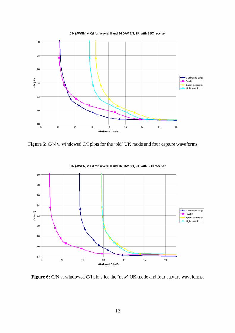
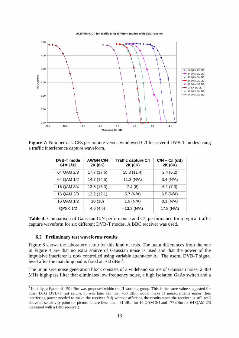
Figures 5 and 6 show C/N v. windowed C/I plots for the two DTT modes currently radiated in the UK. A first generation BBC DVB-T receiver without II countermeasures was used for these measurements. Similar plots were obtained for another two DVB-T receivers. The shape of the curves is very similar. The only difference is the actual performance values but the same conclusions as for the BBC receiver can be drawn. Plots for another three DVB-T modes are shown in Appendix B.

As II is reduced in the system, the C/N asymptotically approaches the value associated to the AWGN failure point which, for the receiver used in these tests, is 17.6 dB and 13.3 dB for 64 QAM rate 2/3 (old UK mode) and 16 QAM rate 3/4 (new UK mode), respectively. Thus, the improvement of the new UK mode over the old UK mode for an AWGN channel is approximately 4 dB, much as expected.

As II is added, system performance starts to be dominated by the impulsive noise instead of the Gaussian noise. This area corresponds to the bends in all curves. When most of the noise bucket in the old UK mode is filled with II (vertical asymptotes), the new UK mode still allows for an increase in I before the receiver fails. When II is the only source of impairment (C/N tends to infinity), we can measure the raw improvement in C/I obtained with a change to the new UK mode. Obviously, this improvement is lower bounded by the 4 dB measured for an AWGN channel. For captures with very high peak to mean power ratios (e.g. traffic interference), clipping effects start to take place in the receiver and an improvements of up to 8 dB can be obtained with the new UK mode.

The major drawback of this approach is the limited isolation of the SMIQ (~54 dB). When the peak to mean ratio of the simulated II is very high, noise from the SMIQ’s DAC breaks through, filling the noise bucket of the DTT receiver and affecting the measurements. A second limitation of this approach is the bandwidth of the interfering signal (only about 20 MHz). The II working group considered that this approach might be useful for chip manufacturers to develop counter measures for 8 MHz circuitry. However, to be representative and for test and development of the whole UHF receiver, the bandwidth of the interfering signal should ideally cover the whole UHF band.

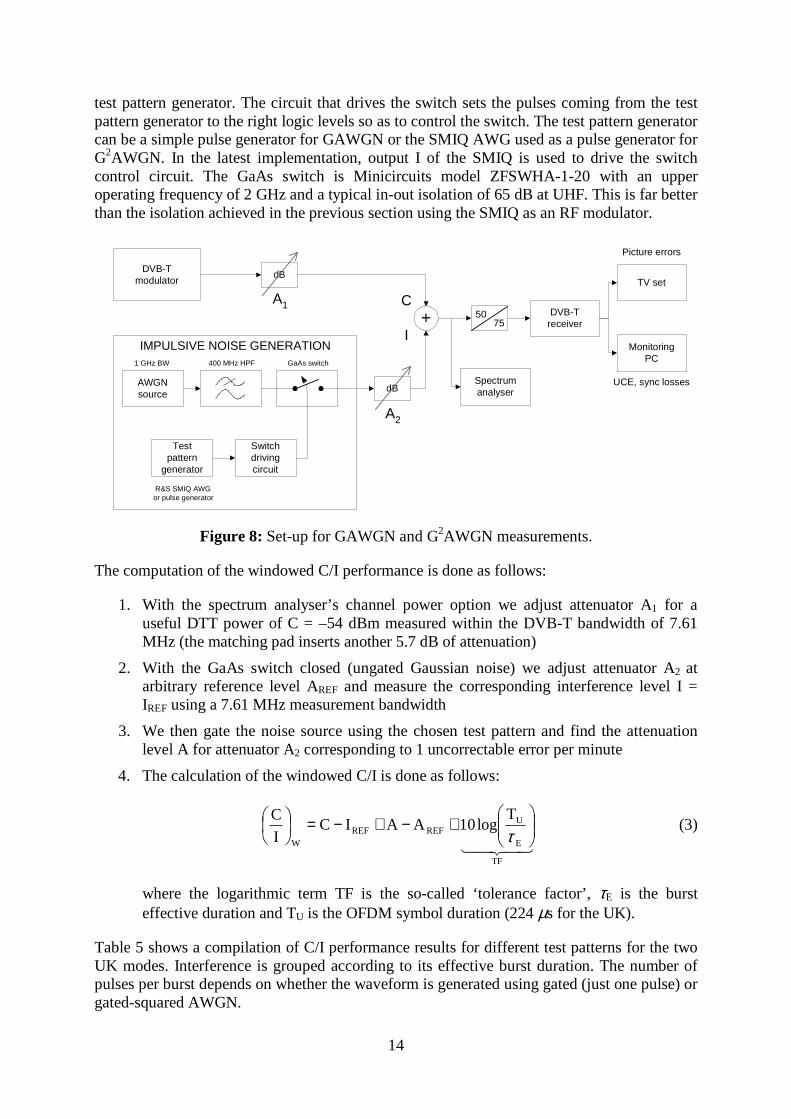
Figure 7 presents some performance results for the captured traffic interference in a different way. No additional Gaussian noise is used this time, and the number of UCE per minute is noted for each level of interference. The failure criterion is 1 UCE per minute (0 in a logarithmic scale). Table 4 shows a comparison of the AWGN C/N values for picture failure and the analogous C/I values extracted from Figure 7.

The advantage of going from 2K to 8K for the two UK modes ranges from 1.5 to 4 dB. To this value we have to add another 6 dB that are not accounted for in the windowed C/I. The disparity between the AWGN C/N and the C/I for traffic is greater for more robust modes. For these modes we need very high peak interference levels to break the system. The limited isolation of the SMIQ means that these high levels cannot be achieved because too much spurious noise gets to the receiver.

12

C/N (AWGN) v. C/I for several II and 64 QAM 2/3, 2K, with BBC receiver

18

20

22

24

26

28

30

14 15 16 17 18 19 20 21 22

Windowed C/I (dB)

C/N

(dB

) Central Heating

Traffic

Spark generator

Light switch

Figure 5: C/N v. windowed C/I plots for the ‘old’ UK mode and four capture waveforms.


14

16

18

20

22

24

26

28

30

7 9 11 13 15 17 19

Windowed C/I (dB)

C/N

(dB

) Central Heating

Traffic

Spark generator

Light switch

Figure 6: C/N v. windowed C/I plots for the ‘new’ UK mode and four capture waveforms.

13

UCE/min v. C/I for Traffic II for different modes with BBC receiver

-1.00

0.00

1.00

2.00

3.00

4.00

5.00

-21.0 -16.0 -11.0 -6.0 -1.0 4.0 9.0 14.0

Windowed C/I (dB)

log

UC

E/m

in

64 QAM 2/3 2K

64 QAM 1/2 2K

16 QAM 3/4 2K

16 QAM 2/3 2K

16 QAM 1/2 2K

QPSK 1/2 2K

16 QAM 3/4 8K

64 QAM 2/3 8K

Figure 7: Number of UCEs per minute versus windowed C/I for several DVB-T modes using a traffic interference capture waveform.

DVB-T mode

GI = 1/32 AWGN C/N

2K (8K) Traffic capture C/I

2K (8K) C/N – C/I (dB)

2K (8K)

64 QAM 2/3 17.7 (17.6) 15.3 (11.4) 2.4 (6.2)

64 QAM 1/2 14.7 (14.5) 11.3 (N/A) 3.4 (N/A)

16 QAM 3/4 13.5 (13.3) 7.4 (6) 6.1 (7.3)

16 QAM 2/3 12.2 (12.1) 5.7 (N/A) 6.5 (N/A)

16 QAM 1/2 10 (10) 1.9 (N/A) 8.1 (N/A)

QPSK 1/2 4.6 (4.5) –13.3 (N/A) 17.9 (N/A)

Table 4: Comparison of Gaussian C/N performance and C/I performance for a typical traffic capture waveform for six different DVB-T modes. A BBC receiver was used.

6.2 Preliminary test waveforms results

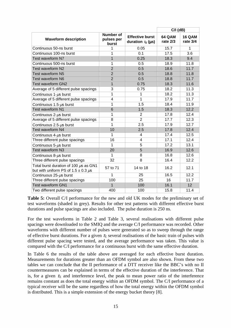
Figure 8 shows the laboratory setup for this kind of tests. The main differences from the one in Figure 4 are that no extra source of Gaussian noise is used and that the power of the impulsive interferer is now controlled using variable attenuator A2. The useful DVB-T signal level after the matching pad is fixed at –60 dBm8.

The impulsive noise generation block consists of a wideband source of Gaussian noise, a 400 MHz high-pass filter that eliminates low frequency noise, a high isolation GaAs switch and a

__________________________________________________________________________________________ 8 Initially, a figure of –50 dBm was proposed within the II working group. This is the same value suggested for other DTG DVB-T test setups. It was later felt that –60 dBm would make II measurements easier (less interfering power needed to make the receiver fail) without affecting the results since the receiver is still well above its sensitivity point for picture failure (less than –81 dBm for 16 QAM 3/4 and –77 dBm for 64 QAM 2/3 measured with a BBC receiver).

14

test pattern generator. The circuit that drives the switch sets the pulses coming from the test pattern generator to the right logic levels so as to control the switch. The test pattern generator can be a simple pulse generator for GAWGN or the SMIQ AWG used as a pulse generator for G2AWGN. In the latest implementation, output I of the SMIQ is used to drive the switch control circuit. The GaAs switch is Minicircuits model ZFSWHA-1-20 with an upper operating frequency of 2 GHz and a typical in-out isolation of 65 dB at UHF. This is far better than the isolation achieved in the previous section using the SMIQ as an RF modulator.

DVB-Tmodulator

dB

IMPULSIVE NOISE GENERATION

AWGNsource

1 GHz BW 400 MHz HPF GaAs switch

Testpattern

generator

Switchdrivingcircuit

R&S SMIQ AWGor pulse generator

dB

+C

I

5075

DVB-Treceiver

MonitoringPC

UCE, sync losses

TV set

Picture errors

Spectrumanalyser

A1

A2

Figure 8: Set-up for GAWGN and G2AWGN measurements.

The computation of the windowed C/I performance is done as follows:

1. With the spectrum analyser’s channel power option we adjust attenuator A1 for a useful DTT power of C = –54 dBm measured within the DVB-T bandwidth of 7.61 MHz (the matching pad inserts another 5.7 dB of attenuation)

2. With the GaAs switch closed (ungated Gaussian noise) we adjust attenuator A2 at arbitrary reference level AREF and measure the corresponding interference level I = IREF using a 7.61 MHz measurement bandwidth

3. We then gate the noise source using the chosen test pattern and find the attenuation level A for attenuator A2 corresponding to 1 uncorrectable error per minute

4. The calculation of the windowed C/I is done as follows:

��TF

E

UREFREF

W

Tlog10AAIC

I

C��

��

�+−+−=�

�

��

�

τ (3)

where the logarithmic term TF is the so-called ‘ tolerance factor’ , τE is the burst effective duration and TU is the OFDM symbol duration (224 µs for the UK).

Table 5 shows a compilation of C/I performance results for different test patterns for the two UK modes. Interference is grouped according to its effective burst duration. The number of pulses per burst depends on whether the waveform is generated using gated (just one pulse) or gated-squared AWGN.

15

C/I (dB)

Waveform description Number of pulses per

burst

Effective burst duration τE (µµµµs)

64 QAM rate 2/3

16 QAM rate 3/4

Continuous 50-ns burst 1 0.05 15.7 1 Continuous 100-ns burst 1 0.1 17.5 3.6 Test waveform N7 1 0.25 18.3 9.4 Continuous 500-ns burst 1 0.5 18.9 11.8 Test waveform N2 2 0.5 18.6 11.7 Test waveform N5 2 0.5 18.8 11.8 Test waveform N6 2 0.5 18.8 11.7 Test waveform GN2 1 0.75 18.3 11.6 Average of 5 different pulse spacings 3 0.75 18.2 11.3 Continuous 1-µs burst 1 1 18.2 11.3 Average of 5 different pulse spacings 4 1 17.9 11.7 Continuous 1.5-µs burst 1 1.5 18.4 11.9 Test waveform N1 6 1.5 18.3 12.2 Continuous 2-µs burst 1 2 17.8 12.4 Average of 5 different pulse spacings 8 2 17.7 12.3 Continuous 2.5-µs burst 1 2.5 17.9 12.7 Test waveform N4 10 2.5 17.8 12.4 Continuous 4-µs burst 1 4 17.4 12.5 Three different pulse spacings 16 4 17.1 12.4 Continuous 5-µs burst 1 5 17.2 13.1 Test waveform N3 20 5 16.9 12.6 Continuous 8-µs burst 1 8 16.8 12.6 Three different pulse spacings 32 8 16.4 12.2 Total burst duration of 100 µs as GN1 but with uniform PS of 1.5 ± 0.3 µs

57 to 71 14 to 18 16.2 12.1

Continuous 25-µs burst 1 25 16.5 12.2 Three different pulse spacings 100 25 16 11.7 Test waveform GN1 1 100 16.1 12 Two different pulse spacings 400 100 15.8 11.4

Table 5: Overall C/I performance for the new and old UK modes for the preliminary set of test waveforms (shaded in grey). Results for other test patterns with different effective burst durations and pulse spacings are also included. The pulse duration is 250 ns.

For the test waveforms in Table 2 and Table 3, several realisations with different pulse spacings were downloaded to the SMIQ and the average C/I performance was recorded. Other waveforms with different number of pulses were generated so as to sweep through the range of effective burst durations. For a given τE several realisations of the basic train of pulses with different pulse spacing were tested, and the average performance was taken. This value is compared with the C/I performance for a continuous burst with the same effective duration.

In Table 6 the results of the table above are averaged for each effective burst duration. Measurements for durations greater than an OFDM symbol are also shown. From these two tables we can conclude that the II performance of a DTT receiver like the BBC’s with no II countermeasures can be explained in terms of the effective duration of the interference. That is, for a given τE and interference level, the peak to mean power ratio of the interference remains constant as does the total energy within an OFDM symbol. The C/I performance of a typical receiver will be the same regardless of how the total energy within the OFDM symbol is distributed. This is a simple extension of the energy bucket theory [8].

16

Effective burst duration ττττE (µµµµs)

C/I for 64 QAM rate 2/3

C/I for 16 QAM rate 3/4 C/I (dB)

0.05 15.7 1 14.7 0.1 17.5 3.6 13.9

0.25 18.3 9.4 8.9 0.5 18.8 11.8 7

0.75 18.3 11.4 6.9 1 18.1 11.5 6.6

1.5 18.3 12 6.3 2 17.8 12.3 5.5

2.5 17.8 12.5 5.3 4 17.2 12.5 4.7 5 17.1 12.8 4.3 8 16.6 12.4 4.2 16 16.2 12.1 4.1 25 16.3 12 4.3

100 16 11.8 4.2 200 16 11.7 4.3 300 16.1 11.9 4.2 500 16.8 12.4 4.4 1000 17.3 13.1 4.2 5000 17.6 13.4 4.2

Table 6: Averaged windowed C/I performance for the two UK DTT modes for different effective burst durations. The right-most column represents the C/I improvement for the new UK mode with respect the old UK mode.

The right-most column in Table 6 shows the average II improvement obtained from the change of DTT mode in the UK. This improvement ranges from approximately 4 dB for AWGN to more than 10 dB for impulsive interference with very high peak to mean ratios (in this latter case clipping effects occur in the front end and part of the interference power is thrown away before the demodulation process starts).

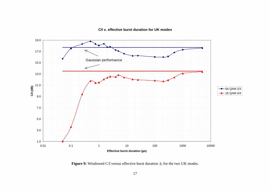
In Figure 9 we show the plots of windowed C/I performance versus effective burst duration for the two UK modes. The AWGN performance of the BBC receiver is also shown as solid lines. As τE increases the C/I asymptotically approaches the AWGN C/N. For bursts shorter than an OFDM symbol but longer than 0.5 µs, the C/I performance is roughly within a 2-dB neighbourhood of the Gaussian performance. For pulses shorter than half a microsecond, clipping occurs in the front end and the behaviour of the receiver departs from the Gaussian performance.

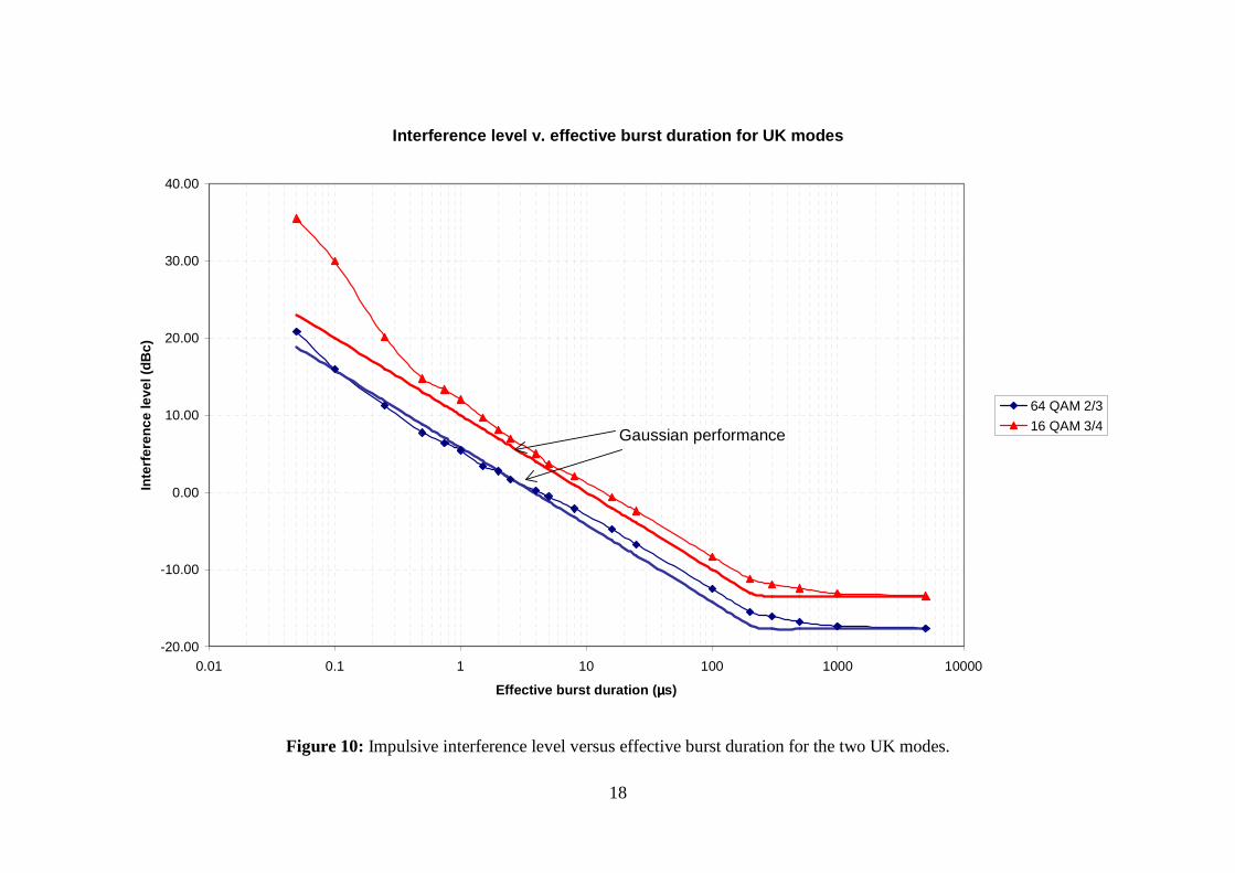
The same results are plotted in Figure 10 but now the amplitude of the interferer is referred to the carrier level. The departure from Gaussian performance is more clearly seen in this figure. The straight line for effective burst durations lesser than an OFDM symbol period has a –3 dB per octave characteristic. That is, doubling the burst duration implies halving the burst amplitude. For effective burst durations greater than an OFDM symbol period, the amplitude approaches that for a Gaussian channel.

The main advantage of using the test setup in Figure 8 to simulate II is that the wide flat power spectrum of the generated interference makes for a fairly easy power calibration and performance measurement. Also, the randomness introduced by the source of noise partly counters the deterministic generation of the test patterns using SMIQ’s arbitrary waveform generator. With gated Gaussian noise we can recreate the basic characteristics of impulsive interference: Wideband spectrum and high peak to mean power ratio.

17

C/I v. effective burst duration for UK modes

1.0

3.0

5.0

7.0

9.0

11.0

13.0

15.0

17.0

19.0

0.01 0.1 1 10 100 1000 10000

Effective burst duration (µµµµs)

C/I

(dB

)

64 QAM 2/3

16 QAM 3/4

Gaussian performance

Figure 9: Windowed C/I versus effective burst duration τE for the two UK modes.

18

Interference level v. effective burst duration for UK modes

-20.00

-10.00

0.00

10.00

20.00

30.00

40.00

0.01 0.1 1 10 100 1000 10000

Effective burst duration (µµµµs)

Inte

rfer

ence

leve

l (d

Bc)

64 QAM 2/3

16 QAM 3/4Gaussian performance

Figure 10: Impulsive interference level versus effective burst duration for the two UK modes.

19

7 DTG impulsive noise test waveforms

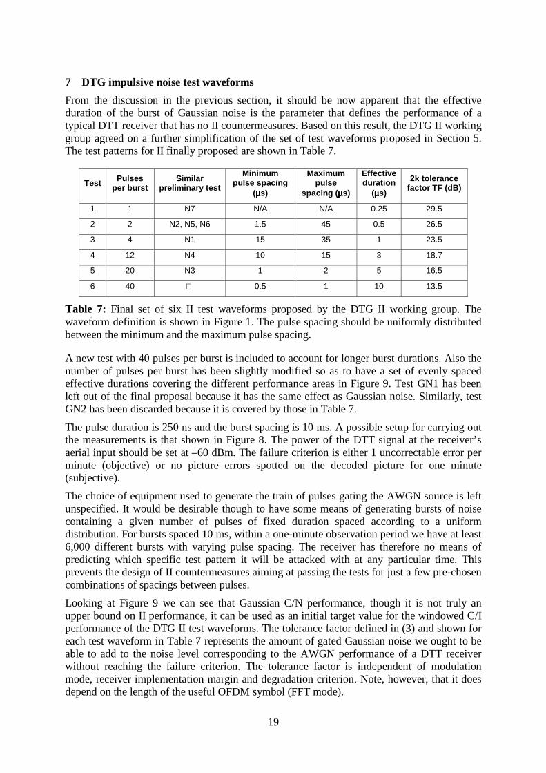
From the discussion in the previous section, it should be now apparent that the effective duration of the burst of Gaussian noise is the parameter that defines the performance of a typical DTT receiver that has no II countermeasures. Based on this result, the DTG II working group agreed on a further simplification of the set of test waveforms proposed in Section 5. The test patterns for II finally proposed are shown in Table 7.

Test Pulses per burst

Similar preliminary test

Minimum pulse spacing

(µµµµs)

Maximum pulse

spacing (µµµµs)

Effective duration

(µµµµs)

2k tolerance factor TF (dB)

1 1 N7 N/A N/A 0.25 29.5

2 2 N2, N5, N6 1.5 45 0.5 26.5

3 4 N1 15 35 1 23.5

4 12 N4 10 15 3 18.7

5 20 N3 1 2 5 16.5

6 40 0.5 1 10 13.5

Table 7: Final set of six II test waveforms proposed by the DTG II working group. The waveform definition is shown in Figure 1. The pulse spacing should be uniformly distributed between the minimum and the maximum pulse spacing.

A new test with 40 pulses per burst is included to account for longer burst durations. Also the number of pulses per burst has been slightly modified so as to have a set of evenly spaced effective durations covering the different performance areas in Figure 9. Test GN1 has been left out of the final proposal because it has the same effect as Gaussian noise. Similarly, test GN2 has been discarded because it is covered by those in Table 7.

The pulse duration is 250 ns and the burst spacing is 10 ms. A possible setup for carrying out the measurements is that shown in Figure 8. The power of the DTT signal at the receiver’s aerial input should be set at –60 dBm. The failure criterion is either 1 uncorrectable error per minute (objective) or no picture errors spotted on the decoded picture for one minute (subjective).

The choice of equipment used to generate the train of pulses gating the AWGN source is left unspecified. It would be desirable though to have some means of generating bursts of noise containing a given number of pulses of fixed duration spaced according to a uniform distribution. For bursts spaced 10 ms, within a one-minute observation period we have at least 6,000 different bursts with varying pulse spacing. The receiver has therefore no means of predicting which specific test pattern it will be attacked with at any particular time. This prevents the design of II countermeasures aiming at passing the tests for just a few pre-chosen combinations of spacings between pulses.

Looking at Figure 9 we can see that Gaussian C/N performance, though it is not truly an upper bound on II performance, it can be used as an initial target value for the windowed C/I performance of the DTG II test waveforms. The tolerance factor defined in (3) and shown for each test waveform in Table 7 represents the amount of gated Gaussian noise we ought to be able to add to the noise level corresponding to the AWGN performance of a DTT receiver without reaching the failure criterion. The tolerance factor is independent of modulation mode, receiver implementation margin and degradation criterion. Note, however, that it does depend on the length of the useful OFDM symbol (FFT mode).

20

For instance, let us assume that the Gaussian performance of a receiver for picture failure is 20 dB for a certain DVB-T mode. The anticipated picture failure point for test waveform 6 should correspond to an ungated noise power equal or greater to –20 dBc + 13.5 dB = –6.5 dBc. A receiver with measures to counter impulsive interference should be expected to perform better than that.

8 Conclusions

This white paper has presented the work carried out by the BBC as leading member of the working group set up within the DTG to study impulsive interference. The aim of this group was to propose a set of realistic and repeatable tests to assess the performance of a DTT receiver suffering from impulsive interference.

As a result of the statistical analysis of a large amount of captures of impulsive interference, we concluded that an effective yet not too simplistic way of simulating impulsive noise was using the well-known gated Gaussian noise model. We have introduced a variation on this model which is the use of a train of gating pulses with constant amplitude and duration but whose spacing is random and follows a uniform distribution. This simulation model has been renamed ‘gated-squared’ Gaussian noise model.

The finally agreed set of tests consists of six waveform patterns with different number of 250-ns pulses which are randomly spaced. These waveforms gate a wideband source of Gaussian noise and must be repeated every 10 ms. The suggested observation period is one minute and the failure criterion is that there can be no more than 1 uncorrectable error per minute. An alternative subjective criterion when this figure is not available is the onset of errors on the decoded picture. We also presented a possible impulsive interference test setup including the type of equipment needed and a recommended measurement method.

The campaign of laboratory measurements used to validate the use of the proposed test waveforms to simulate impulsive interference also yielded other results:

• A 4 to 10 dB improvement in impulsive interference performance obtained with the change from the old UK DTT mode (64 QAM, rate 2/3, 2K and 1/32 guard interval) to the new UK mode (16 QAM, rate 3/4, 2K and 1/32) was measured. This improvement is at least equivalent to the difference in Gaussian noise performance but, depending on the exact nature of the interference, may be up to 6 dB greater.

• It was shown that we need just a single parameter to determine the impulsive noise performance of a DTT receiver equipped with no special countermeasures. That is, for pulsed impulsive interferers receiver performance depends on how many samples of a particular OFDM symbol are affected by the interference, not on how many pulses are present or how they are distributed in the time domain

Acknowledgements

The authors would both like to thank the other contributors within the DTG Impulsive Interference Working Group for their input and useful discussions, in particular Peter Lewis and Vu Pham from Philips Semiconductors who have also developed a capture system in order to analyse engine ignition interference.

Personal acknowledgement by John Salter

As Chairman of the DTG II Working Group, I would like to thank José for his significant contribution to the work of this group.

21

Glossary

ADC Analogue-to-Digital Converter

AP Pulse Amplitude

APD Pulse Amplitude probability Distribution

AWG Arbitrary Waveform Generator

AWGN Additive White Gaussian Noise

BD Burst Duration

BDD Burst Duration probability Distribution

BS Burst Spacing

BSD Burst Spacing probability Distribution

C/I Carrier to Interference Ratio

C/N Carrier to Noise Ratio

DAC Digital-to-Analogue Converter

DTG Digital Television Group

DTT Digital Terrestrial Television

DVB-T Digital Video Broadcasting Terrestrial

ED Event Duration

EDD Event Duration probability Distribution

EMC Electromagnetic Compatibility

GAWGN Gated AWGN

G2AWGN Gated squared or gated gated AWGN

II Impulsive Interference

NAD Noise Amplitude Distribution

OFDM Orthogonal Frequency Division Multiplex

PD Pulse Duration

PDD Pulse Duration probability Distribution

PS Pulse Spacing

PSD Pulse Spacing probability Distribution

QAM Quadrature Amplitude Modulation

TF Tolerance Factor

UCE UnCorrectable Errors

22

References

1. A. Shukla, “Radiocommunications Agency – Feasibility study into the measurement of man-made noise” , DERA/KIS/COM/CR10470, March 2001.

2. M.C. Jeruchim, P. Balaban, K.S. Shanmugan, Simulation of Communication Systems: Modelling, Methodology, and Techniques, 2nd Ed., Kluwer Academic / Plenum Publishers, August 2000.

3. K.L. Blackard, T.S. Rappaport, and C.W. Bostian, “Measurements and Models of Radio Frequency Impulsive Noise for Indoor Wireless Communications”, IEEE Journal on Selected Areas in Comms., Vol. 11, No. 7, September 1993.

4. P. Lewis, “A Tutorial on Impulsive Noise in COFDM Systems” , DTG Monograph No. 5, Digital TV Group, 2001.

5. M.G. Sánchez, L. de Haro, M.C. Ramón, A. Mansilla, C.M. Ortega, D. Oliver, “ Impulsive Noise Measurements and Characterization in a UHF Digital TV Channel” , IEEE Trans. On Electromagnetic Compatibility, Vol. 41, No.2, May 1999.

6. W.R. Lauber, J.M. Bertrand, “Statistics of Motor Vehicle Ignition Noise at VHF/UHF” , IEEE Trans. On Electromagnetic Compatibility, Vol. 41, No. 3, August 1999.

7. J. Salter, J. Lago-Fernández, “DTT Comparison of 64QAM(2/3) with 16QAM(3/4): Co-channel Interference from PAL, Echoes and Impulsive Interference” , BBC R&D White Paper WHP 056, March 2003.

8. R. Poole, “DVB-T Transmission, Reception and Measurement” , DTG Monograph No. 4, Digital TV Group, 2001.

23

A Sample captures and histograms for impulsive interference

This appendix contains the histograms of the II captures used to define the set of test waveforms.

Capture files produced by the capture system are plotted using Octave. Waveforms can be plotted as real signals centred on 4.57 MHz with 7.61 MHz bandwidth or after a second down conversion to their complex baseband equivalent. The down conversion is done directly by multiplying the IF signal by a complex exponential with frequency 4.57 MHz and filtering the resulting waveform with a 28-th order Chebyshev type II low pass filter with a stop band cut-off of –40 dB at 4 MHz. The cut-off frequency is about 3.93 MHz and the filter keeps the average power of the signal.

Prior to the statistical analysis, visual inspection was used to catalogue all captured data. First, data was grouped according to the interfering source. Second, for each source captures showing similar characteristics were grouped together to facilitate the analysis. The validity of this approach can be questioned because of its subjectivity, but given the chaotic nature of impulsive interference, some subjective pre-processing is needed in order to glean anything useful from the statistical analysis.

In the statistical analysis we generate histograms that approximate the probability density function (pdf) for the pulse amplitude (Amplitude Probability Distribution, APD), pulse duration (PDD), pulse spacing (PSD), burst duration (BDD), burst spacing (BSD) and event duration (EDD) for each of the pre-defined II categories. These are the parameters shown in Figure 1 (there it is further assumed that all pulses have the same amplitude).

Captured waveforms are first downconverted to complex baseband in order to facilitate the statistical analysis. We use the magnitude of the envelope of the resulting complex waveform to estimate the parameters in model (1). This eliminates the additional ringing in the capture waveform caused by the 4.57 MHz modulating carrier, making it easier to identify the different statistical parameters.

The first difficulty we face when trying to extract from a set of captures the statistical distribution of a certain parameter is how we distinguish between the different units that comprise an impulsive event. That is, for instance, when do we decide that a burst is a complete event or that a group of pulses can be called a burst? The following set of thresholds is used in the statistical analysis to tackle this problem:

• PS: Minimum spacing between pulses to avoid mistaking for a new pulse the pulse side lobes still remaining in the capture waveform after pre-processing

• PS2BS: Time threshold above which the spacing between pulses becomes the spacing between bursts. The next pulse will then belong to a new burst

• BS2ES: Time threshold above which a burst within the same capture file is considered to belong to a new impulsive event

• VTHR: Amplitude threshold used to determine where pulses start and end. This is the decision level used to extract the impulse of noise from the background noise of the capture system.

Even after the introduction of these thresholds, for some interfering sources we still found it hard to subjectively determine what a burst or event is.

24

In the capture waveforms pulses correspond to the impulse response of the complete downconversion process (from the aerial input to complex baseband). A typical plot of the complex envelope of this impulse response is shown in Figure A-1. The spacing between the main peak and the main first lobe is about 8 samples (200 ns) whilst the spacing between the latter and the second lobe is 6 samples (150 ns).

0

50

100

150

200

0 0.2 0.4 0.6 0.8 1

Env

elop

e am

plitu

de (

mV

)

Elapsed time (us)

Snapshot taken at Thu Nov 22 11:50:51 2001. Captured range: 134737.490 to 134738.565 us

Figure A-1: Magnitude of the complex impulse response of the tuner used in the capture system.

The information about the timing of the side lobes is used in the analysis to remove all spurious side lobes introduced by the impulse response of the tuner, leaving only the main lobes for subsequent analysis. The identification of side lobes relies more on the spacing between them than on their relative amplitudes. This is so because the former is less likely to be affected by non-linearities in the first stages of the front end and/or system noise.

In the following sections we present the histograms for fourteen types of impulsive interference. The APD approximates the distribution of the peak values of the impulse response’s main lobe. The pulse duration is calculated taking into account both the rising and falling tails of the main lobe. BDD and EDD are only shown here expressed in pulses per burst and bursts per event, respectively. Other way of presenting these two histograms would be using time units. Vector MAX sets the abscissa’s upper limit for each histogram plot.

Between brackets and above each histogram we show the mean value for the distribution and its standard deviation expressed as a percentage of the average value.

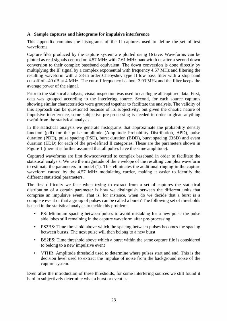
A.1 Central Heating type 1 (CH thermostat switches on)

A sample capture belonging to this group is shown in Figure A-2. The histograms obtained from the analysis of all captured data under this category are shown in Figure A-3. Visually the interference is made of noise-like long impulsive bursts.

Most events contain just one burst. The average pulse duration is 260 ns and pulses are very close to each other. Bursts span less than half a millisecond and contain several hundred pulses. As far as DVB-T is concerned, this interferer resembles Gaussian noise.

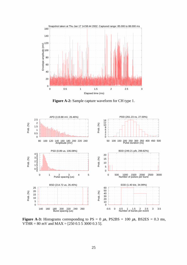
25

0

20

40

60

80

100

120

140

160

0 0.5 1 1.5 2 2.5 3

Env

elop

e am

plitu

de (

mV

)

Elapsed time (ms)

Snapshot taken at Thu Jan 17 14:58:44 2002. Captured range: 85.000 to 88.000 ms

Figure A-2: Sample capture waveform for CH type 1.

00.5

11.5

22.5

80 100 120 140 160 180 200 220 240

Pro

b. (

%)

Amplitude (mV)

APD (119.88 mV, 26.46%)

02468

101214

50 100 150 200 250 300 350 400 450 500

Pro

b. (

%)

Pulse duration (ns)

PDD (261.23 ns, 27.00%)

00.5

11.5

22.5

33.5

44.5

0 1 2 3 4 5

Pro

b. (

%)

Pulse spacing (us)

PSD (0.89 us, 106.08%)

0

5

10

15

20

0 500 1000 1500 2000 2500 3000

Pro

b. (

%)

Number of pulses per burst

BDD (249.21 p/b, 299.82%)

05

10152025

140 160 180 200 220 240 260

Pro

b. (

%)

Burst spacing (us)

BSD (214.72 us, 26.45%)

0102030405060

-0.5 0 0.5 1 1.5 2 2.5 3 3.5

Pro

b. (

%)

Number of bursts per event

EDD (1.40 b/e, 34.99%)

Figure A-3: Histograms corresponding to PS = 0 µs, PS2BS = 100 µs, BS2ES = 0.3 ms, VTHR = 80 mV and MAX = [250 0.5 5 3000 0.3 5].

26

A.2 Central Heating type 2 (CH thermostat switches on or off)

Another group of captures obtained from central heating thermostats look like the one in Figure A-4. The corresponding histograms are displayed in Figure A-5. Bursts are spiky and rather short (~150 µs) and contain a few pulses whose frequency repetition is in the range of a few tens of kHz. An event consists of just one burst.

0

50

100

150

200

0 0.1 0.2 0.3 0.4 0.5 0.6 0.7 0.8 0.9 1

Env

elop

e am

plitu

de (

mV

)

Elapsed time (ms)

Snapshot taken at Tue Oct 16 11:47:21 2001. Captured range: 94.000 to 95.000 ms


012345

100 200 300 400 500 600

Pro

b. (

%)

Amplitude (mV)

APD (192.31 mV, 81.35%)

05

10152025

150 200 250 300 350 400 450 500

Pro

b. (

%)

Pulse duration (ns)

PDD (318.75 ns, 18.89%)

01234567

0 20 40 60 80 100

Pro

b. (

%)

Pulse spacing (us)

PSD (30.41 us, 76.74%)

05

101520253035

0 2 4 6 8 10 12

Pro

b. (

%)


BDD (6.00 p/b, 75.15%)

020406080

100

-0.5 0 0.5 1 1.5 2 2.5

Pro

b. (

%)


EDD (1.00 b/e, 0.00%)

Figure A-5: Histograms corresponding to PS = 1.2 µs, PS2BS = 140 µs, BS2ES = 1 ms, VTHR = 65 mV and MAX = [650 0.5 140 20 1 10].

27

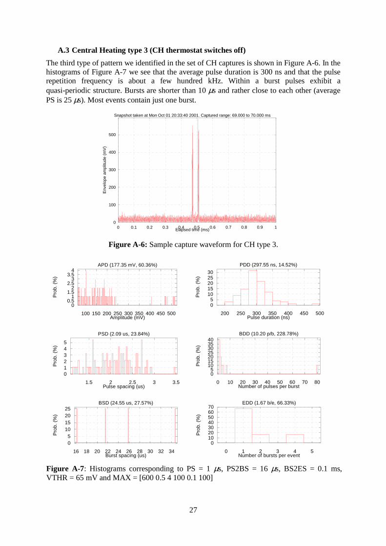
A.3 Central Heating type 3 (CH thermostat switches off)

The third type of pattern we identified in the set of CH captures is shown in Figure A-6. In the histograms of Figure A-7 we see that the average pulse duration is 300 ns and that the pulse repetition frequency is about a few hundred kHz. Within a burst pulses exhibit a quasi-periodic structure. Bursts are shorter than 10 µs and rather close to each other (average PS is 25 µs). Most events contain just one burst.

0

100

200

300

400

500

0 0.1 0.2 0.3 0.4 0.5 0.6 0.7 0.8 0.9 1

Env

elop

e am

plitu

de (

mV

)

Elapsed time (ms)

Snapshot taken at Mon Oct 01 20:33:40 2001. Captured range: 69.000 to 70.000 ms


00.5

11.5

22.5

33.5

4

100 150 200 250 300 350 400 450 500

Pro

b. (

%)

Amplitude (mV)

APD (177.35 mV, 60.36%)

05

1015202530

200 250 300 350 400 450 500

Pro

b. (

%)

Pulse duration (ns)

PDD (297.55 ns, 14.52%)

012345

1.5 2 2.5 3 3.5

Pro

b. (

%)

Pulse spacing (us)

PSD (2.09 us, 23.84%)

05

10152025303540

0 10 20 30 40 50 60 70 80

Pro

b. (

%)


BDD (10.20 p/b, 228.78%)

05

10152025

16 18 20 22 24 26 28 30 32 34

Pro

b. (

%)

Burst spacing (us)

BSD (24.55 us, 27.57%)

010203040506070

0 1 2 3 4 5

Pro

b. (

%)


EDD (1.67 b/e, 66.33%)

Figure A-7: Histograms corresponding to PS = 1 µs, PS2BS = 16 µs, BS2ES = 0.1 ms, VTHR = 65 mV and MAX = [600 0.5 4 100 0.1 100]

28

A.4 Cooker ignition

The spark generated by the electronic ignition system in a cooker induces the sort of waveform shown in Figure A-8. The histograms obtained from the statistical analysis are shown in Figure A-9. Pulses are an average of 290 ns long and are spaced by 1 or 2 µs, although some scattered pulses can be spotted as well. Events amount to bursts and last about 40 µs. The number of pulses per burst varies, but typically it is less than 20.

0

50

100

150

200

250

300

350

400

0 0.1 0.2 0.3 0.4 0.5 0.6 0.7 0.8 0.9 1

Env

elop

e am

plitu

de (

mV

)

Elapsed time (ms)


Figure A-8: Sample capture waveform for cooker ignition system.

0

0.5

1

1.5

2

100 200 300 400 500 600

Pro

b. (

%)

Amplitude (mV)

APD (182.87 mV, 43.00%)

02468

1012141618

50 100 150 200 250 300 350 400 450 500

Pro

b. (

%)

Pulse duration (ns)

PDD (288.36 ns, 23.42%)

00.5

11.5

22.5

33.5

44.5

1 2 3 4 5 6 7 8

Pro

b. (

%)

Pulse spacing (us)

PSD (1.73 us, 66.26%)

05

10152025

0 10 20 30 40 50 60 70 80

Pro

b. (

%)


BDD (24.17 p/b, 96.55%)

020406080

100

-0.5 0 0.5 1 1.5 2 2.5

Pro

b. (

%)


EDD (1.00 b/e, 0.00%)

Figure A-9: Histograms corresponding to PS = 0.975 µs, PS2BS = 30 µs, BS2ES = 0.1 ms, VTHR = 90 mV and MAX = [600 0.5 8 100 0.1 100].

29

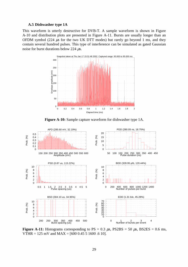
A.5 Dishwasher type 1A

This waveform is utterly destructive for DVB-T. A sample waveform is shown in Figure A-10 and distribution plots are presented in Figure A-11. Bursts are usually longer than an OFDM symbol (224 µs for the two UK DTT modes) but rarely go beyond 1 ms, and they contain several hundred pulses. This type of interference can be simulated as gated Gaussian noise for burst durations below 224 µs.

0

50

100

150

200

250

300

0 0.2 0.4 0.6 0.8 1 1.2 1.4 1.6 1.8 2

Env

elop

e am

plitu

de (

mV

)

Elapsed time (ms)


Figure A-10: Sample capture waveform for dishwasher type 1A.

00.10.20.30.40.5

150 200 250 300 350 400 450 500 550 600

Pro

b. (

%)

Amplitude (mV)

APD (285.60 mV, 32.19%)

0

5

10

15

20

50 100 150 200 250 300 350 400 450

Pro

b. (

%)

Pulse duration (ns)

PDD (280.05 ns, 18.75%)

02468

10

0.5 1 1.5 2 2.5 3 3.5 4 4.5 5

Pro

b. (

%)

Pulse spacing (us)

PSD (0.87 us, 115.22%)

02468

10

0 200 400 600 800 1000 1200 1400

Pro

b. (

%)


BDD (328.95 p/b, 120.44%)

02468

10

200 250 300 350 400 450 500

Pro

b. (

%)

Burst spacing (us)

BSD (304.10 us, 34.95%)

010203040506070

0 1 2 3 4

Pro

b. (

%)


EDD (1.31 b/e, 45.28%)

Figure A-11: Histograms corresponding to PS = 0.3 µs, PS2BS = 50 µs, BS2ES = 0.6 ms, VTHR = 125 mV and MAX = [600 0.45 5 1600 .6 10].

30

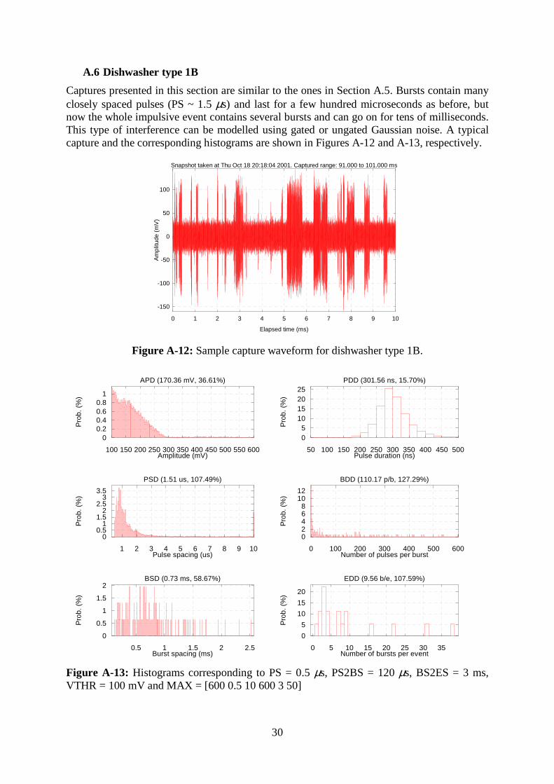
A.6 Dishwasher type 1B

Captures presented in this section are similar to the ones in Section A.5. Bursts contain many closely spaced pulses (PS ~ 1.5 µs) and last for a few hundred microseconds as before, but now the whole impulsive event contains several bursts and can go on for tens of milliseconds. This type of interference can be modelled using gated or ungated Gaussian noise. A typical capture and the corresponding histograms are shown in Figures A-12 and A-13, respectively.

-150

-100

-50

0

50

100

0 1 2 3 4 5 6 7 8 9 10

Am

plitu

de (

mV

)

Elapsed time (ms)

Snapshot taken at Thu Oct 18 20:18:04 2001. Captured range: 91.000 to 101.000 ms

Figure A-12: Sample capture waveform for dishwasher type 1B.

00.20.40.60.8

1

100 150 200 250 300 350 400 450 500 550 600

Pro

b. (

%)

Amplitude (mV)

APD (170.36 mV, 36.61%)

05

10152025

50 100 150 200 250 300 350 400 450 500

Pro

b. (

%)

Pulse duration (ns)

PDD (301.56 ns, 15.70%)

00.5

11.5

22.5

33.5

1 2 3 4 5 6 7 8 9 10

Pro

b. (

%)

Pulse spacing (us)

PSD (1.51 us, 107.49%)

02468

1012

0 100 200 300 400 500 600

Pro

b. (

%)


BDD (110.17 p/b, 127.29%)

0

0.5

1

1.5

2

0.5 1 1.5 2 2.5

Pro

b. (

%)

Burst spacing (ms)

BSD (0.73 ms, 58.67%)

0

5

10

15

20

0 5 10 15 20 25 30 35

Pro

b. (

%)


EDD (9.56 b/e, 107.59%)

Figure A-13: Histograms corresponding to PS = 0.5 µs, PS2BS = 120 µs, BS2ES = 3 ms, VTHR = 100 mV and MAX = [600 0.5 10 600 3 50]

31

A.7 Diswasher type 2

Captures in this section exhibit a more repeatable behaviour and it is relatively easier to extract a common pattern. The PSD peaks at 11 and 19.5 µs and the total duration of the bursts is on average 330 µs. Bursts are spaced by 900 µs and there are between 1 and 3 bursts per event.

0

50

100

150

200

0 0.1 0.2 0.3 0.4 0.5 0.6 0.7 0.8 0.9 1

Env

elop

e am

plitu

de (

mV

)

Elapsed time (ms)

Snapshot taken at Thu Oct 18 20:15:50 2001. Captured range: 71.000 to 72.000 ms

Figure A-14: Sample capture waveform for dishwasher type 2.

00.5

11.5

22.5

100 200 300 400 500 600

Pro

b. (

%)

Amplitude (mV)

APD (170.28 mV, 62.75%)

05

10152025

100 200 300 400 500 600

Pro

b. (

%)

Pulse duration (ns)

PDD (319.61 ns, 19.10%)

00.5

11.5

22.5

3

0 20 40 60 80 100 120 140 160 180 200

Pro

b. (

%)

Pulse spacing (us)

PSD (24.50 us, 128.07%)

02468

1012141618

0 10 20 30 40 50 60 70 80

Pro

b. (

%)


BDD (14.50 p/b, 146.30%)

02468

101214

0.4 0.6 0.8 1 1.2 1.4 1.6

Pro

b. (

%)

Burst spacing (ms)

BSD (0.87 ms, 51.70%)

01020304050

0 1 2 3 4

Pro

b. (

%)


EDD (1.78 b/e, 51.54%)

Figure A-15: Histograms corresponding to PS = 2 µs, PS2BS = 200 µs, BS2ES = 2 ms, VTHR = 70 mV and MAX = [700 0.6 200 100 2 10]

32

A.8 Dishwasher type 3

This third type of capture produced by a dishwasher is characterised by long noise-like bursts of variable duration containing hundreds of pulses with repetition frequencies of the order of several hundred hertz. Events almost always correspond to one burst and can be modelled as Gaussian noise. A sample capture is shown in Figure A-16 and the histograms are plotted in Figure A-17.

0

50

100

150

200

250

0 0.2 0.4 0.6 0.8 1 1.2 1.4 1.6 1.8 2

Env

elop

e am

plitu

de (

mV

)

Elapsed time (ms)

Snapshot taken at Mon Oct 01 20:09:20 2001. Captured range: 92.000 to 94.000 ms

Figure A-16: Sample capture waveform for dishwasher type 3.

0

0.5

1

1.5

2

100 150 200 250 300 350

Pro

b. (

%)

Amplitude (mV)

APD (111.63 mV, 42.17%)

0

5

10

15

20

50 100 150 200 250 300 350 400 450 500

Pro

b. (

%)

Pulse duration (ns)

PDD (295.42 ns, 18.31%)

00.5

11.5

22.5

5 10 15 20 25 30

Pro

b. (

%)

Pulse spacing (us)

PSD (4.42 us, 102.22%)

02468

10121416

0 200 400 600 800 1000 1200 1400

Pro

b. (

%)


BDD (347.69 p/b, 126.27%)

01020304050

182 184 186 188 190 192

Pro

b. (

%)

Burst spacing (us)

BSD (187.00 us, 1.87%)

01020304050607080

-0.5 0 0.5 1 1.5 2 2.5 3 3.5

Pro

b. (

%)


EDD (1.18 b/e, 32.64%)


33

A.9 Light switch off type 1

The first type of impulsive interference captured after throwing a light switch spans several OFDM symbols and thus, from the point of view of a DTT receiver, it is equivalent to Gaussian noise. However its internal structure is more complex. The PSD is almost continuous, peaking at 1.45, 1.8 and 2.45 µs. There are two types of bursts: those shorter than 800 µs containing several hundred pulses and those lasting between 2 and 4 ms with several thousand pulses per burst. Short bursts come usually alone. Long bursts form events of usually two bursts each separated by around 10 ms. Figures A-18 and A-19 show two sample capture waveforms and the histograms for this capture category.

0

50

100

150

200

250

0 2 4 6 8 10 12 14 16 18

Env

elop

e am

plitu

de (

mV

)

Elapsed time (us)

0

50

100

150

200

250

300

350

400

450

0 0.5 1 1.5 2 2.5 3 3.5 4 4.5 5

Env

elop

e am

plitu

de (

mV

)

Elapsed time (ms)

Snapshot taken at Wed Jan 23 21:46:24 2002. Captured range: 155.000 to 160.000 ms

Figure A-18: Sample capture waveforms for light switch off type 1.

00.10.20.30.40.50.60.70.80.9

100 150 200 250 300 350 400 450 500

Pro

b. (

%)

Amplitude (mV)

APD (369.53 mV, 22.55%)

05

10152025

50 100 150 200 250 300 350 400 450

Pro

b. (

%)

Pulse duration (ns)

PDD (330.97 ns, 13.69%)

012345678

1 1.5 2 2.5 3 3.5 4

Pro

b. (

%)

Pulse spacing (us)

PSD (1.72 us, 31.66%)

012345

0 500 1000 1500 2000 2500

Pro

b. (

%)


BDD (816.16 p/b, 108.27%)

02468

10121416

2 4 6 8 10

Pro

b. (

%)

Burst spacing (ms)

BSD (8.78 ms, 34.29%)

01020304050607080

0 2 4 6 8 10 12

Pro

b. (

%)


EDD (1.95 b/e, 131.69%)


34

A.10 Light switch off type 2

This other set of captures corresponding to light switches being thrown off is characterised by long spiky bursts which form events not stretching beyond 10 ms. Two captures representative of this group and the associated histograms are show in Figure A-20 and Figure A-21, respectively. Some figures seem to repeatedly crop up for the spacing between bursts (1, 2, 4 and 10 ms). Bursts contain only a few pulses which are rather close to each other.

0

50

100

150

200

250

300

350

400

0 10 20 30 40 50 60 70 80

Env

elop

e am

plitu

de (

mV

)

Elapsed time (us) 0

50

100

150

200

0 0.1 0.2 0.3 0.4 0.5 0.6 0.7 0.8 0.9 1E

nvel

ope

ampl

itude

(m

V)

Elapsed time (ms)

Snapshot taken at Wed Jan 23 21:46:24 2002. Captured range: 114.000 to 115.000 ms

Figure A-20: Sample capture waveforms for light switch off type 2.

0

0.5

1

1.5

2

100 150 200 250 300 350 400

Pro

b. (

%)

Amplitude (mV)

APD (145.62 mV, 47.14%)

0

5

10

15

20

100 150 200 250 300 350 400 450 500

Pro

b. (

%)

Pulse duration (ns)

PDD (310.51 ns, 17.82%)

00.5

11.5

22.5

33.5

0 20 40 60 80 100

Pro

b. (

%)

Pulse spacing (us)

PSD (13.80 us, 150.23%)

02468

1012141618

0 10 20 30 40 50 60

Pro

b. (

%)


BDD (11.28 p/b, 109.34%)

02468

101214

0 2 4 6 8 10 12 14 16

Pro

b. (

%)

Burst spacing (ms)

BSD (2.11 ms, 167.64%)

05

10152025

0 2 4 6 8 10

Pro

b. (

%)


EDD (3.00 b/e, 64.46%)

Figure A-21: Histograms corresponding to PS = 1 µs, PS2BS = 120 µs, BS2ES = 20 ms, VTHR = 70 mV and MAX = [450 0.5 120 100 18 20].

35

A.11 Fluorescent/low-energy lights switched on

For this group of captures pulses are spaced by an average of 45 µs and bursts contain between 1 and 4 pulses. There are usually one or two bursts per event and bursts are separated by about half a millisecond. The corresponding plots are shown in Figures A-22 and A-23.

0

50

100

150

200

250

300

0 0.5 1 1.5 2 2.5 3

Env

elop

e am

plitu

de (

mV

)

Elapsed time (ms)


Figure A-22: Sample capture waveform for fluorescent lights switched on.

0

0.5

1

1.5

2

100 200 300 400 500 600 700

Pro

b. (

%)

Amplitude (mV)

APD (355.61 mV, 52.14%)

02468

1012141618

150 200 250 300 350 400 450 500 550 600

Pro

b. (

%)

Pulse duration (ns)

PDD (346.56 ns, 17.87%)

00.5

11.5

22.5

50 100 150 200

Pro

b. (

%)

Pulse spacing (us)

PSD (44.55 us, 104.95%)

05

10152025

0 2 4 6 8 10 12 14 16

Pro

b. (

%)


BDD (3.35 p/b, 83.49%)

00.5

11.5

22.5

33.5

44.5

0.3 0.4 0.5 0.6 0.7 0.8 0.9 1 1.1

Pro

b. (

%)

Burst spacing (ms)

BSD (0.55 ms, 44.96%)

01020304050

0 1 2 3 4 5

Pro

b. (

%)


EDD (1.76 b/e, 55.18%)

Figure A-23: Histograms corresponding to PS = 5 µs, PS2BS = 250 µs, BS2ES = 2 ms, VTHR = 100 mV and MAX = [700 0.6 250 100 1.5 10]

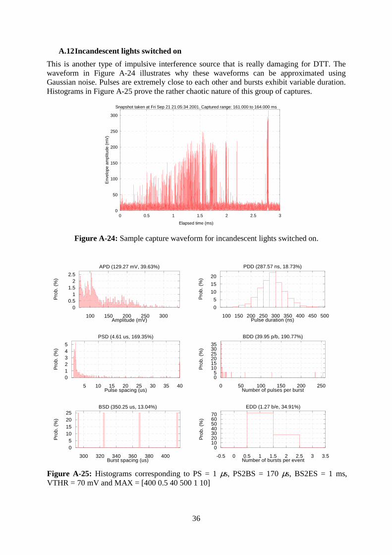
36

A.12 Incandescent lights switched on

This is another type of impulsive interference source that is really damaging for DTT. The waveform in Figure A-24 illustrates why these waveforms can be approximated using Gaussian noise. Pulses are extremely close to each other and bursts exhibit variable duration. Histograms in Figure A-25 prove the rather chaotic nature of this group of captures.

0

50

100

150

200

250

300

0 0.5 1 1.5 2 2.5 3

Env

elop

e am

plitu

de (

mV

)

Elapsed time (ms)

Snapshot taken at Fri Sep 21 21:05:34 2001. Captured range: 161.000 to 164.000 ms

Figure A-24: Sample capture waveform for incandescent lights switched on.

00.5

11.5

22.5

100 150 200 250 300

Pro

b. (

%)

Amplitude (mV)

APD (129.27 mV, 39.63%)

0

5

10

15

20

100 150 200 250 300 350 400 450 500

Pro

b. (

%)

Pulse duration (ns)

PDD (287.57 ns, 18.73%)

012345

5 10 15 20 25 30 35 40

Pro

b. (

%)

Pulse spacing (us)

PSD (4.61 us, 169.35%)

05

101520253035

0 50 100 150 200 250

Pro

b. (

%)


BDD (39.95 p/b, 190.77%)

05

10152025

300 320 340 360 380 400

Pro

b. (

%)

Burst spacing (us)

BSD (350.25 us, 13.04%)

010203040506070

-0.5 0 0.5 1 1.5 2 2.5 3 3.5

Pro

b. (

%)


EDD (1.27 b/e, 34.91%)


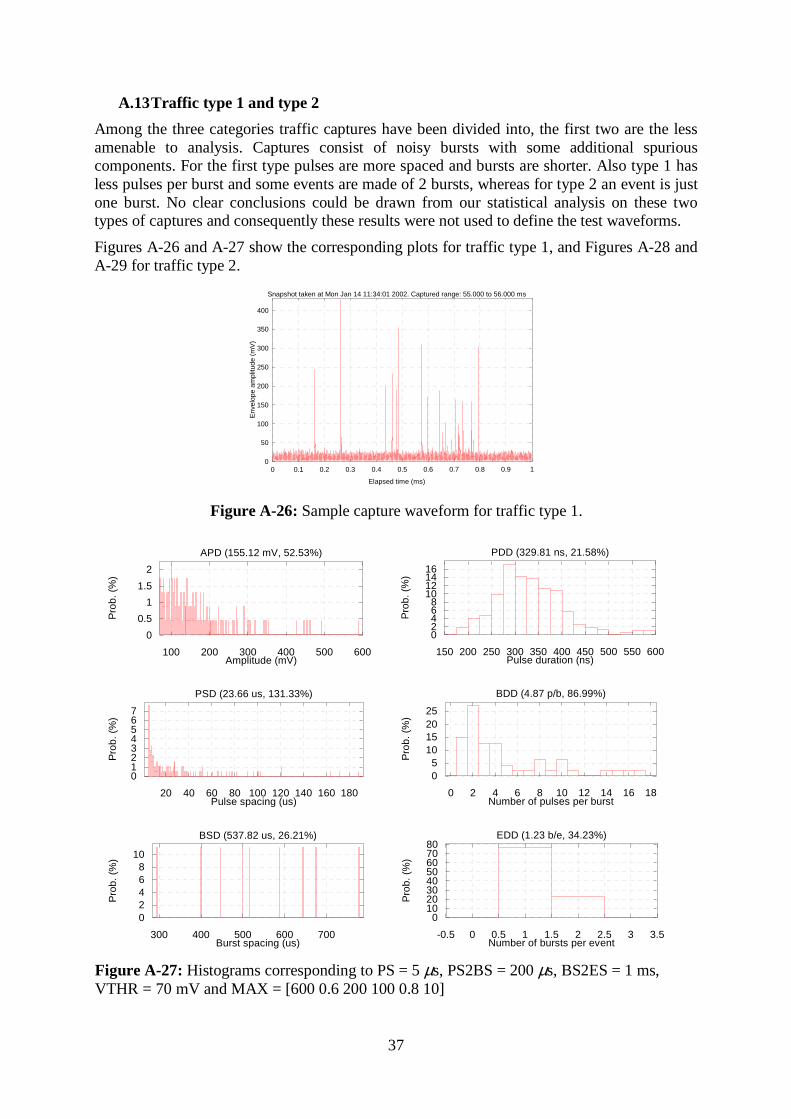
37

A.13 Traffic type 1 and type 2

Among the three categories traffic captures have been divided into, the first two are the less amenable to analysis. Captures consist of noisy bursts with some additional spurious components. For the first type pulses are more spaced and bursts are shorter. Also type 1 has less pulses per burst and some events are made of 2 bursts, whereas for type 2 an event is just one burst. No clear conclusions could be drawn from our statistical analysis on these two types of captures and consequently these results were not used to define the test waveforms.

Figures A-26 and A-27 show the corresponding plots for traffic type 1, and Figures A-28 and A-29 for traffic type 2.

0

50

100

150

200

250

300

350

400

0 0.1 0.2 0.3 0.4 0.5 0.6 0.7 0.8 0.9 1

Env

elop

e am

plitu

de (

mV

)

Elapsed time (ms)

Snapshot taken at Mon Jan 14 11:34:01 2002. Captured range: 55.000 to 56.000 ms

Figure A-26: Sample capture waveform for traffic type 1.

0

0.5

1

1.5

2

100 200 300 400 500 600

Pro

b. (

%)

Amplitude (mV)

APD (155.12 mV, 52.53%)

02468

10121416

150 200 250 300 350 400 450 500 550 600

Pro

b. (

%)

Pulse duration (ns)

PDD (329.81 ns, 21.58%)

01234567

20 40 60 80 100 120 140 160 180

Pro

b. (

%)

Pulse spacing (us)

PSD (23.66 us, 131.33%)

05

10152025

0 2 4 6 8 10 12 14 16 18

Pro

b. (

%)


BDD (4.87 p/b, 86.99%)

02468

10

300 400 500 600 700

Pro

b. (

%)

Burst spacing (us)

BSD (537.82 us, 26.21%)

01020304050607080

-0.5 0 0.5 1 1.5 2 2.5 3 3.5

Pro

b. (

%)


EDD (1.23 b/e, 34.23%)

Figure A-27: Histograms corresponding to PS = 5 µs, PS2BS = 200 µs, BS2ES = 1 ms, VTHR = 70 mV and MAX = [600 0.6 200 100 0.8 10]

38

0

20

40

60

80

100

120

0 0.1 0.2 0.3 0.4 0.5 0.6 0.7 0.8 0.9 1

Env

elop

e am

plitu

de (

mV

)

Elapsed time (ms)


Figure A-28: Sample capture waveform for traffic type 2.

00.5

11.5

22.5

33.5

44.5

60 80 100 120 140 160 180

Pro

b. (

%)

Amplitude (mV)

APD (81.15 mV, 21.35%)

0

5

10

15

20

100 150 200 250 300 350 400 450 500 550 600

Pro

b. (

%)

Pulse duration (ns)

PDD (315.48 ns, 23.05%)

012345

20 40 60 80 100 120

Pro

b. (

%)

Pulse spacing (us)

PSD (9.68 us, 129.51%)

02468

1012141618

0 20 40 60 80 100 120 140

Pro

b. (

%)


BDD (22.00 p/b, 156.94%)

020406080

100

-0.5 0 0.5 1 1.5 2 2.5

Pro

b. (

%)


EDD (1.00 b/e, 0.00%)


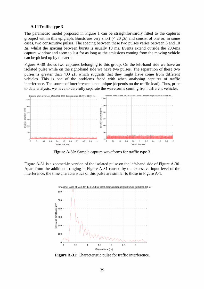
39

A.14 Traffic type 3

The parametric model proposed in Figure 1 can be straightforwardly fitted to the captures grouped within this epigraph. Bursts are very short (< 20 µs) and consist of one or, in some cases, two consecutive pulses. The spacing between these two pulses varies between 5 and 10 µs, whilst the spacing between bursts is usually 10 ms. Events extend outside the 200-ms capture window and seem to last for as long as the emissions coming from the moving vehicle can be picked up by the aerial.

Figure A-30 shows two captures belonging to this group. On the left-hand side we have an isolated pulse while on the right-hand side we have two pulses. The separation of these two pulses is greater than 400 µs, which suggests that they might have come from different vehicles. This is one of the problems faced with when analysing captures of traffic interference. The source of interference is not unique (depends on the traffic load). Thus, prior to data analysis, we have to carefully separate the waveforms coming from different vehicles.

0

100

200

300

400

500

600

0 0.1 0.2 0.3 0.4 0.5 0.6 0.7 0.8 0.9 1

Env

elop

e am

plitu

de (

mV

)

Elapsed time (ms)


0

50

100

150

200

250

300

0 0.2 0.4 0.6 0.8 1 1.2 1.4 1.6 1.8 2

Env

elop

e am

plitu

de (

mV

)

Elapsed time (ms)


Figure A-30: Sample capture waveforms for traffic type 3.

Figure A-31 is a zoomed-in version of the isolated pulse on the left-hand side of Figure A-30. Apart from the additional ringing in Figure A-31 caused by the excessive input level of the interference, the time characteristics of this pulse are similar to those in Figure A-1.

0

100

200

300

400

500

600

0 0.5 1 1.5 2 2.5 3

Env

elop

e am

plitu

de (

mV

)

Elapsed time (us)

Snapshot taken at Mon Jan 14 11:54:12 2002. Captured range: 85606.500 to 85609.975 us

Figure A-31: Characteristic pulse for traffic interference.

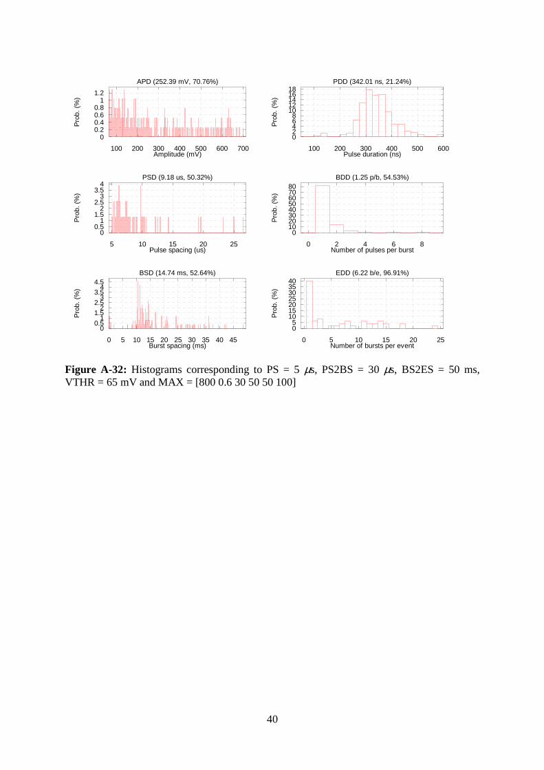
40

00.20.40.60.8

11.2

100 200 300 400 500 600 700

Pro

b. (

%)

Amplitude (mV)

APD (252.39 mV, 70.76%)

02468

1012141618

100 200 300 400 500 600

Pro

b. (

%)

Pulse duration (ns)

PDD (342.01 ns, 21.24%)

00.5

11.5

22.5

33.5

4

5 10 15 20 25

Pro

b. (

%)

Pulse spacing (us)

PSD (9.18 us, 50.32%)

01020304050607080

0 2 4 6 8

Pro

b. (

%)


BDD (1.25 p/b, 54.53%)

00.5

11.5

22.5

33.5

44.5

0 5 10 15 20 25 30 35 40 45

Pro

b. (

%)

Burst spacing (ms)

BSD (14.74 ms, 52.64%)

05

10152025303540

0 5 10 15 20 25

Pro

b. (

%)


EDD (6.22 b/e, 96.91%)


41

B Additional DVB-T II performance plots for capture waveforms + SMIQ

Figures B-1 to B-4 show the normalised amplitude of the complex baseband II captures used in Section 6.1.

0

0.2

0.4

0.6

0.8

1

0 50 100 150 200

Nor

mal

ised

am

plitu

de

Time (us)

Figure B-1: Capture waveform of central heating interference.

0

0.2

0.4

0.6

0.8

1

0 1 2 3 4 5 6 7 8 9

Nor

mal

ised

am

plitu

de

Time (us)

Figure B-2: Capture of traffic interference.

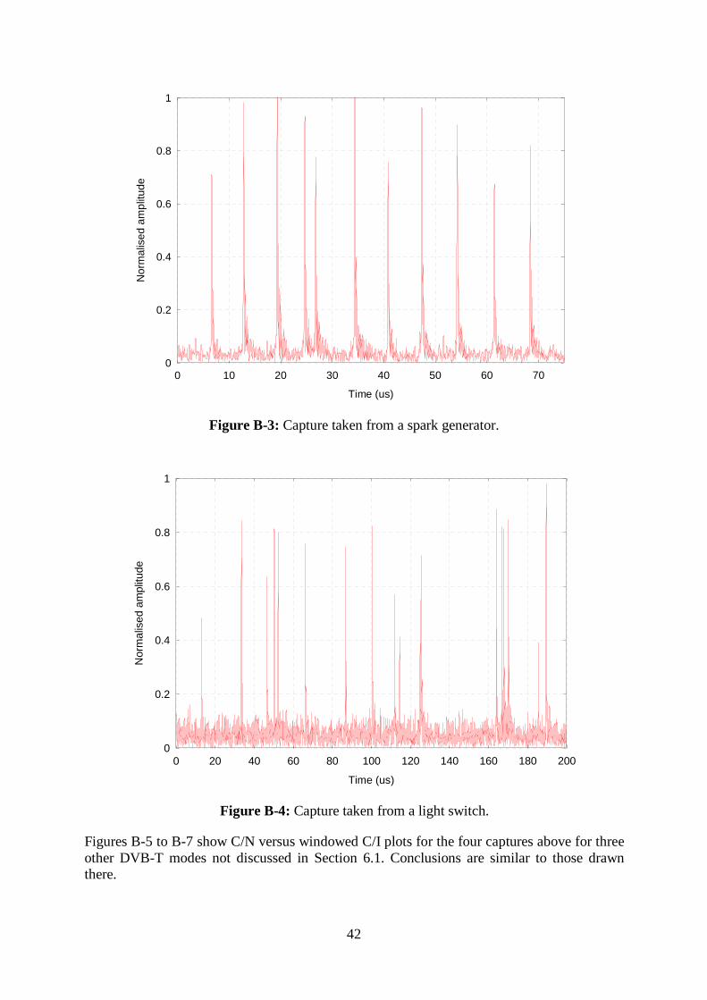
42

0

0.2

0.4

0.6

0.8

1

0 10 20 30 40 50 60 70

Nor

mal

ised

am

plitu

de

Time (us)

Figure B-3: Capture taken from a spark generator.

0

0.2

0.4

0.6

0.8

1

0 20 40 60 80 100 120 140 160 180 200

Nor

mal

ised

am

plitu

de

Time (us)

Figure B-4: Capture taken from a light switch.

Figures B-5 to B-7 show C/N versus windowed C/I plots for the four captures above for three other DVB-T modes not discussed in Section 6.1. Conclusions are similar to those drawn there.

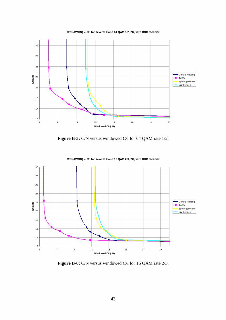
43


15

17

19

21

23

25

27

29

9 11 13 15 17 19 21 23

Windowed C/I (dB)

C/N

(dB

) Central Heating

Traffic

Spark generator

Light switch

Figure B-5: C/N versus windowed C/I for 64 QAM rate 1/2.


12

14

16

18

20

22

24

26

28

30

5 7 9 11 13 15 17 19

Windowed C/I (dB)

C/N

(dB

) Central Heating

Traffic

Spark generator

Light switch


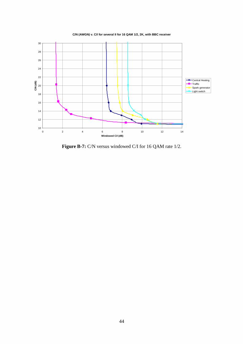
44

C/N (AWGN) v. C/I for several II for 16 QAM 1/2, 2K, with BBC receiver

10

12

14

16

18

20

22

24

26

28

30

0 2 4 6 8 10 12 14

Windowed C/I (dB)

C/N

(dB

) Central Heating

Traffic

Spark generator

Light switch


R&D White Paper - downloads.bbc.co.uk

Documents

Transcript of R&D White Paper - downloads.bbc.co.uk