
Rajesh Vasa -- PhD Thesis
252
Growth and Change Dynamics in Open Source Software Systems Rajesh Vasa A thesis presented for the degree of Doctor of Philosophy 2010
-
Upload
rajeshvasa -
Category
Documents
-
view
222 -
download
0
Transcript of Rajesh Vasa -- PhD Thesis
8/8/2019 Rajesh Vasa -- PhD Thesis
http://slidepdf.com/reader/full/rajesh-vasa-phd-thesis 1/252
Growth and Change Dynamicsin Open Source Software
Systems
Rajesh Vasa
A thesis presented for the degree of Doctor of Philosophy
2010

8/8/2019 Rajesh Vasa -- PhD Thesis
http://slidepdf.com/reader/full/rajesh-vasa-phd-thesis 2/252
Abstract
In this thesis we address the problem of identifying where, in successfulsoftware systems, maintenance effort tends to be devoted. By examin-ing a larger data set of open source systems we show that maintenance
effort is, in general, spent on addition of new classes. Interestingly, ef-forts to base new code on stable classes will make those classes lessstable as they need to be modified to meet the needs of the new clients.
This thesis advances the state of the art in terms of our understandingof how evolving software systems grow and change. We propose aninnovative method to better understand growth dynamics in evolvingsoftware systems. Rather than relying on the commonly used methodof analysing aggregate system size growth over time, we analyze how the probability distribution of a range of software metrics change over time. Using this approach we find that the process of evolution typically drives the popular classes within a software system to gain additionalclients over time and the increase in popularity makes these classeschange-prone.
Furthermore, we show that once a set of classes have been released,they resist change and the modifications that they do undergo are ingeneral, small adaptations rather than substantive rework. The meth-ods we developed to analyze evolution can be used to detect releases
with systemic and architectural changes as well as identify presence of machine generated code.
Finally, we also extend the body of knowledge with respect to validationof the Laws of Software Evolution as postulated by Lehman. We findconsistent support for the applicability of the following laws of softwareevolution: first law Continuing Change , third law Self Regulation , fifthlaw Conservation of Familiarity , and the sixth law Continuing Growth .However, our analysis was unable to find evidence to support the other
laws.
i

8/8/2019 Rajesh Vasa -- PhD Thesis
http://slidepdf.com/reader/full/rajesh-vasa-phd-thesis 3/252
Dedicated to all my teachers
ii

8/8/2019 Rajesh Vasa -- PhD Thesis
http://slidepdf.com/reader/full/rajesh-vasa-phd-thesis 4/252
Acknowledgements
I would like to acknowledge with particular gratitude the assistance of my supervisors, Dr. Jean-Guy Schneider and Dr. Philip Branch. I amalso indebted to a number of other people, in particular, Dr. MarkusLumpe, Prof. Oscar Nierstrasz, Dr. Clinton Woodward, Andrew Cain,Dr. Anthony Tang, Samiran Muhmud, Joshua Hayes and Ben Hall whocollaborated with me on various research papers and provided muchneeded support. Thanks also to the various developers of open sourcesoftware systems for releasing their software with non-restrictive li-censing. I am grateful to my current employer, Swinburne University of Technology for providing the resources and support to pursue a re-search higher degree.
Finally, I would like to thank my family for their loving forbearance dur-ing the long period it has taken me to conduct the research and writeup this thesis.
Rajesh Vasa, 2010
iii
8/8/2019 Rajesh Vasa -- PhD Thesis
http://slidepdf.com/reader/full/rajesh-vasa-phd-thesis 5/252
Declaration
I declare that this thesis contains no material that has been accepted for the award of any other degree or diploma and to the best of my knowl-edge contains no material previously published or written by another person except where due reference is made in the text of this thesis.
Rajesh Vasa, 2010
iv

8/8/2019 Rajesh Vasa -- PhD Thesis
http://slidepdf.com/reader/full/rajesh-vasa-phd-thesis 6/252
Publications Arising from this
Thesis
The work described in this thesis has been published as described inthe following list:
1. R. Vasa and J.-G. Schneider. Evolution of Cyclomatic Complexity in Object-Oriented Software. In Proceedings of 7th ECOOP Work- shop on Quantitative Approaches in Object-Oriented Software Engi- neering (QAOOSE ’03) , 2003.
2. R. Vasa, J.-G. Schneider, C. Woodward, and A. Cain. DetectingStructural Changes in Object-Oriented Software Systems. In Pro- ceedings of 4th IEEE International Symposium on Empirical Soft- ware Engineering (ISESE ’05) , 2005.
3. R. Vasa, M. Lumpe, and J.-G. Schneider. Patterns of Component Evolution. In Proceedings of the 6th International Symposium on Software Composition (SC ’07) , Springer, 2007.
4. R. Vasa, J.-G. Schneider, and O. Nierstrasz. The Inevitable Stabil-ity of Software Change. In Proceedings of 23rd IEEE International Conference on Software Maintenance (ICSM ’07) , 2007.
5. R. Vasa, J.-G. Schneider, O. Nierstrasz, and C. Woodward. Onthe Resilience of Classes to Change. In Proceedings of 3rd Interna- tional ERCIM Symposium on Software Evolution (Evol ’07) , Volume8. Electronic Communications of the EASST, 2008.
6. A. Tang, J. Han, and R. Vasa. Software Architecture Design Rea-soning: A Case for Improved Methodology Support. IEEE Software ,26(2):43 – 49, 2009.
v

8/8/2019 Rajesh Vasa -- PhD Thesis
http://slidepdf.com/reader/full/rajesh-vasa-phd-thesis 7/252
7. R. Vasa, M. Lumpe, P. Branch, and O. Nierstrasz. Comparative Analysis of Evolving Software Systems using the Gini Coefficient.In Proceedings of the 25th IEEE International Conference on Soft-
ware Maintenance (ICSM ’09) , 2009.
8. M. Lumpe, S. Mahmud, and R. Vasa. On the Use of Propertiesin Java Applications. In Proceedings of the 21st Australian Soft- ware Engineering Conference (ASWEC ’10) . Australian Computer Society, 2010.
Although the thesis is written as a linear document, the actual research work involved substantial exploration, idea formation, modelling, ex-
perimenting and some backtracking as we hit dead-ends. The followingtext outlines how the publications relate to this thesis.
The early articles helped lay the foundation and scope the work pre-sented in this thesis. Specifically, the QAOOSE’03 and ISESE’05 ar-ticles (papers 1 and 2) showed that software metrics typically exhibit highly skewed distributions that retain their shape over time and that architectural changes can be detected by analyzing these changing dis-tributions. The article published at SC’2007 (paper 3) expanded on theISESE’05 article (paper 2) and presented a mathematical model to de-scribe the evolution process and also put forward the thresholds as wellas a technique to detect substantial changes between releases. Thesepapers helped establish and refine the input data selection method(Chapter 3), validate the approach that we take for extracting metrics(Chapter 4), and developed the modelling approach that we eventually used to detect substantial changes between releases (Chapter 5).
More recent work (in particular, ICSM’07 and ICSM’09 articles and theEVOL’07 article – papers 4, 5 and 7) contributed to the content pre-
sented in Chapters 5 and 6 of this thesis which address the primary research questions. The article in ASWEC’10 (paper 8) showed that thekey analysis approach advocated in this thesis can also be used to un-derstand how properties are used in Java software. The IEEE Softwarearticle in 2009 (paper 6) presented a method for reasoning about soft-
ware architecture and the findings from this thesis influenced some of the arguments with respect to the long term stability of software archi-tecture. The implications that we derived from all of the various papersare expanded upon in Chapter 7.
vi

8/8/2019 Rajesh Vasa -- PhD Thesis
http://slidepdf.com/reader/full/rajesh-vasa-phd-thesis 8/252
Contents
1 Introduction 1
1.1 Research Goals . . . . . . . . . . . . . . . . . . . . . . . . . . 4
1.2 Research Approach . . . . . . . . . . . . . . . . . . . . . . . 5
1.3 Main Research Outcomes . . . . . . . . . . . . . . . . . . . . 6
1.4 Thesis Organisation . . . . . . . . . . . . . . . . . . . . . . . 8
2 Software Evolution 10
2.1 Evolution . . . . . . . . . . . . . . . . . . . . . . . . . . . . . 10
2.2 Software Evolution . . . . . . . . . . . . . . . . . . . . . . . . 13
2.3 The Laws of Software Evolution . . . . . . . . . . . . . . . . 18
2.4 Studies of Growth . . . . . . . . . . . . . . . . . . . . . . . . 22
2.5 Studies of Change . . . . . . . . . . . . . . . . . . . . . . . . 30
2.6 Research Questions . . . . . . . . . . . . . . . . . . . . . . . 39
3 Data Selection Methodology 41
3.1 Evolution History . . . . . . . . . . . . . . . . . . . . . . . . 41
3.2 Open Source Software (OSS) . . . . . . . . . . . . . . . . . . 44
3.3 Open Source Project Repositories . . . . . . . . . . . . . . . 46
vii

8/8/2019 Rajesh Vasa -- PhD Thesis
http://slidepdf.com/reader/full/rajesh-vasa-phd-thesis 9/252
C
3.4 Selection Criteria . . . . . . . . . . . . . . . . . . . . . . . . . 47
3.5 Selected Systems - An Overview . . . . . . . . . . . . . . . . 50
3.6 Focus of Study . . . . . . . . . . . . . . . . . . . . . . . . . . 53
3.6.1 Categories of data sources . . . . . . . . . . . . . . . 53
3.6.2 Java Software Systems . . . . . . . . . . . . . . . . . 54
3.7 Summary . . . . . . . . . . . . . . . . . . . . . . . . . . . . . 59
4 Measuring Evolving Software 60
4.1 Measuring Software . . . . . . . . . . . . . . . . . . . . . . . 61
4.2 Types of Metrics . . . . . . . . . . . . . . . . . . . . . . . . . 62
4.2.1 Size Metrics . . . . . . . . . . . . . . . . . . . . . . . . 62
4.2.2 Complexity Metrics . . . . . . . . . . . . . . . . . . . . 63
4.3 Software Evolution History Model . . . . . . . . . . . . . . . 66
4.4 Measuring Time . . . . . . . . . . . . . . . . . . . . . . . . . 67
4.4.1 Release Sequence Number (RSN) . . . . . . . . . . . . 67
4.4.2 Calendar Time . . . . . . . . . . . . . . . . . . . . . . 70
4.5 Metric Extraction . . . . . . . . . . . . . . . . . . . . . . . . 72
4.5.1 Jar Extraction . . . . . . . . . . . . . . . . . . . . . . 73
4.5.2 Class Metric Extraction . . . . . . . . . . . . . . . . . 74
4.5.3 Merge Inner Classes . . . . . . . . . . . . . . . . . . . 82
4.5.4 Class Dependency Graph Construction . . . . . . . . 82
4.5.5 Dependency Metric Extraction . . . . . . . . . . . . . 84
4.5.6 Inheritance Metric Extraction . . . . . . . . . . . . . 88
viii

8/8/2019 Rajesh Vasa -- PhD Thesis
http://slidepdf.com/reader/full/rajesh-vasa-phd-thesis 10/252
C
4.6 Summary . . . . . . . . . . . . . . . . . . . . . . . . . . . . . 89
5 Growth Dynamics 90
5.1 Nature of Software Metric Data . . . . . . . . . . . . . . . . 92
5.1.1 Summarising with Descriptive Statistics . . . . . . . 93
5.1.2 Distribution Fitting to Understand Metric Data . . . 95
5.2 Summarizing Software Metrics . . . . . . . . . . . . . . . . . 98
5.2.1 Gini Coefficient - An Overview . . . . . . . . . . . . . 98
5.2.2 Computing the Gini Coefficient . . . . . . . . . . . . 99
5.2.3 Properties of Gini Coefficient . . . . . . . . . . . . . . 101
5.2.4 Application of the Gini Coefficient - An Example . . 102
5.3 Analysis Approach . . . . . . . . . . . . . . . . . . . . . . . . 103
5.3.1 Metrics Analyzed . . . . . . . . . . . . . . . . . . . . . 103
5.3.2 Metric Correlation . . . . . . . . . . . . . . . . . . . . 104
5.3.3 Checking Shape of Metric Data Distribution . . . . . 105
5.3.4 Computing Gini Coefficient for Java Programs . . . . 106
5.3.5 Identifying the Range of Gini Coefficients . . . . . . . 106
5.3.6 Analysing the Trend of Gini Coefficients . . . . . . . 107
5.4 Observations . . . . . . . . . . . . . . . . . . . . . . . . . . . 109
5.4.1 Correlation between measures . . . . . . . . . . . . . 109
5.4.2 Metric Data Distributions are not Normal . . . . . . 111
5.4.3 Evolution of Metric Distributions . . . . . . . . . . . 111
5.4.4 Bounded Nature of Gini Coefficients . . . . . . . . . 113
ix
8/8/2019 Rajesh Vasa -- PhD Thesis
http://slidepdf.com/reader/full/rajesh-vasa-phd-thesis 11/252
C
5.4.5 Identifying Change using Gini Coefficient . . . . . . 115
5.4.6 Extreme Gini Coefficient Values . . . . . . . . . . . . 117
5.4.7 Trends in Gini Coefficients . . . . . . . . . . . . . . . 118
5.4.8 Summary of Observations . . . . . . . . . . . . . . . 119
5.5 Discussion . . . . . . . . . . . . . . . . . . . . . . . . . . . . 121
5.5.1 Correlation between Metrics . . . . . . . . . . . . . . 122
5.5.2 Dynamics of Growth . . . . . . . . . . . . . . . . . . . 123
5.5.3 Preferential Attachment . . . . . . . . . . . . . . . . . 124
5.5.4 Stability in Software Evolution . . . . . . . . . . . . . 126
5.5.5 Significant Changes . . . . . . . . . . . . . . . . . . . 128
5.5.6 God Classes . . . . . . . . . . . . . . . . . . . . . . . . 130
5.5.7 Value of Gini Coefficient . . . . . . . . . . . . . . . . . 132
5.5.8 Machine-generated Code . . . . . . . . . . . . . . . . 134
5.6 Summary . . . . . . . . . . . . . . . . . . . . . . . . . . . . . 136
6 Change Dynamics 138
6.1 Detecting and Measuring Change . . . . . . . . . . . . . . . 140
6.1.1 Approaches for Detecting Change . . . . . . . . . . . 140
6.1.2 Our Approach for Detecting Change in a Class . . . 142
6.1.3 Identifying Modified, New and Deleted Classes . . . . 143
6.1.4 Measuring Change . . . . . . . . . . . . . . . . . . . . 144
6.1.5 Measuring Popularity and Complexity of a Class . . 145
6.2 Observations . . . . . . . . . . . . . . . . . . . . . . . . . . . 145
x

8/8/2019 Rajesh Vasa -- PhD Thesis
http://slidepdf.com/reader/full/rajesh-vasa-phd-thesis 12/252
C
6.2.1 Probability of Change . . . . . . . . . . . . . . . . . . 146
6.2.2 Rate of Modification . . . . . . . . . . . . . . . . . . . 153
6.2.3 Distribution of the Amount of Change . . . . . . . . 155
6.2.4 Modified Classes and Popularity . . . . . . . . . . . . 157
6.2.5 Modification Probability and In-Degree Count . . . . 159
6.2.6 Popularity of New Classes . . . . . . . . . . . . . . . . 160
6.2.7 Structural Complexity of Modified Classes . . . . . . 162
6.2.8 Summary of Observations . . . . . . . . . . . . . . . 164
6.3 Discussion . . . . . . . . . . . . . . . . . . . . . . . . . . . . 165
6.3.1 Probability of Change . . . . . . . . . . . . . . . . . . 165
6.3.2 Rate and Distribution of Change . . . . . . . . . . . . 167
6.3.3 Popularity of Modified Classes . . . . . . . . . . . . . 168
6.3.4 Popularity of New Classes . . . . . . . . . . . . . . . . 170
6.3.5 Complexity of Modified Classes . . . . . . . . . . . . . 170
6.3.6 Development Strategy and its Impact on Change . . 171
6.4 Related work . . . . . . . . . . . . . . . . . . . . . . . . . . . 174
6.5 Limitations . . . . . . . . . . . . . . . . . . . . . . . . . . . . 179
6.6 Summary . . . . . . . . . . . . . . . . . . . . . . . . . . . . . 180
7 Implications 181
7.1 Laws of Software Evolution . . . . . . . . . . . . . . . . . . . 181
7.2 Software Development Practices . . . . . . . . . . . . . . . . 186
7.2.1 Project Management . . . . . . . . . . . . . . . . . . . 186
xi

8/8/2019 Rajesh Vasa -- PhD Thesis
http://slidepdf.com/reader/full/rajesh-vasa-phd-thesis 13/252
C
7.2.2 Software Metric Tools . . . . . . . . . . . . . . . . . . 188
7.2.3 Testing and Monitoring Changes . . . . . . . . . . . . 189
7.2.4 Competent programmer hypothesis . . . . . . . . . . 190
7.2.5 Creating Reusable Software Components . . . . . . . 191
7.3 Summary . . . . . . . . . . . . . . . . . . . . . . . . . . . . . 192
8 Conclusions 193
8.1 Contributions . . . . . . . . . . . . . . . . . . . . . . . . . . . 193
8.2 Future Work . . . . . . . . . . . . . . . . . . . . . . . . . . . 195
A Meta Data Collected for Software Systems 199
B Raw Metric Data 200
C Mapping between Metrics and Java Bytecode 201
D Metric Extraction Illustration 202
E Growth Dynamics Data Files 204
F Change Dynamics Data Files 205
References 207
xii

8/8/2019 Rajesh Vasa -- PhD Thesis
http://slidepdf.com/reader/full/rajesh-vasa-phd-thesis 14/252
List of Figures
2.1 The process of evolution. . . . . . . . . . . . . . . . . . . . . 12
2.2 The different types of growth rates observed in evolvingsoftware systems. . . . . . . . . . . . . . . . . . . . . . . . . 23
2.3 Illustration of the segmented growth in the Groovy lan-guage compiler. The overall growth rate appears to besuper-linear, with two distinct sub-linear segments. . . . . 27
3.1 Component diagram of a typical software system in our study. Only the Core System JAR components (highlighted
in the image) are investigated and used for the metric ex-traction process. . . . . . . . . . . . . . . . . . . . . . . . . . 55
4.1 UML Class diagram of evolution history model. . . . . . . . 66
4.2 Time intervals (measured in days) between releases is er-ratic. . . . . . . . . . . . . . . . . . . . . . . . . . . . . . . . . 69
4.3 Cumulative distribution showing the number of releasesover the time interval between releases. . . . . . . . . . . . 70
4.4 Age is calculated in terms of the days elapsed since first release. . . . . . . . . . . . . . . . . . . . . . . . . . . . . . . 71
4.5 The metric extraction process for each release of a softwaresystem . . . . . . . . . . . . . . . . . . . . . . . . . . . . . . . 72
4.6 The dependency graph that is constructed includes classesfrom the core, external libraries and the Java framework.
The two sets, N and K, used in our dependency graph pro-
cessing are highlighted in the figure. . . . . . . . . . . . . . 83
xiii

8/8/2019 Rajesh Vasa -- PhD Thesis
http://slidepdf.com/reader/full/rajesh-vasa-phd-thesis 15/252
L F
4.7 Class diagram showing dependency information to illus-trate how dependency metrics are computed. The metricsfor the various classes shown in the table below the diagram 86
4.8 Class diagram to illustrate how inheritance metrics arecomputed. The metrics for the diagram shown in the table
below the diagram. . . . . . . . . . . . . . . . . . . . . . . . . 88
5.1 Relative and Cumulative frequency distribution showingpositively skewed metrics data for the Spring Framework 2.5.3. The right y-axis shows the cumulative percentage,
while the left side shows the relative percentage. . . . . . . 93
5.2 Change in Median value for 3 metrics in PMD. . . . . . . . 95
5.3 Lorenz curve for Out-Degree Count in Spring framework inrelease 2.5.3. . . . . . . . . . . . . . . . . . . . . . . . . . . . 100
5.4 Correlation coefficient distributions across all systems andreleases. The top graph shows the box-plots for each of the 10 metrics under analysis. The bottom graph plotsthe distribution for the metrics. . . . . . . . . . . . . . . . . 108
5.5 Spring evolution profiles showing the upper and lower bound-aries on the relative frequency distributions for Number of Branches , In-Degree Count , Number of Methods and Out- Degree Count . All metric values during the entire evolutionof 5 years fall within the boundaries shown. The y-axis inall the charts shows the percentage of classes (similar toa histogram). . . . . . . . . . . . . . . . . . . . . . . . . . . . 112
5.6 The distinct change in shape of the profile for Hibernateframework between the three major releases. Major re-
leases were approximately 2 years apart. . . . . . . . . . . . 113
5.7 Box plot of Gini coefficients across all selected Java systems.115
5.8 IDC Gini evolution for Struts. . . . . . . . . . . . . . . . . . 116
5.9 Evolution of selected Gini coefficients in Spring. The high-lighted sections are discussed in Section 5.4.5. . . . . . . . 117
5.10Box plot of Gini coefficients correlated with Age . . . . . . . 120
xiv
8/8/2019 Rajesh Vasa -- PhD Thesis
http://slidepdf.com/reader/full/rajesh-vasa-phd-thesis 16/252
L F
5.11Correlation between Number of Branches and all other mea-sures in Proguard. Box plots show the range and distribu-tion of the correlation coefficients over the release history. 122
5.12Evolution of Type Construction Count for ProGuard. . . . . 129
5.13NOB Gini profile for JabRef. . . . . . . . . . . . . . . . . . . 134
6.1 Change evolution in the Hibernate framework. This graphillustrates change property captured by Equation 6.2.9. . . 148
6.2 Change evolution in the Hibernate framework. This graphillustrates change property captured by Equation 6.2.10. . 149
6.3 Box plot of system maturity showing distribution of age(in days since birth) and if the change properties hold.Graph on the left covers Equation 6.2.9, while the right side graph covers Equation 6.2.10. . . . . . . . . . . . . . . 150
6.4 Probability of change reduces with system maturity. Graphon the left indicates the probability that Equation 6.2.9holds, while the right side graph indicates probability for Equation 6.2.10. The probabilities were predicted from the
Logistic regression models. Age indicates days since birth. 151
6.5 Cumulative distribution of the modification frequency of classes that have undergone a change in their lifetime.
The figure only shows some systems from our data set toimprove readability. Systems that are considered outliershave been shown with dotted lines . . . . . . . . . . . . . . 154
6.6 Number of measures that change for modified classes. x-axis shows the number of measures that have been mod-
ified, while the y-axis shows the percentage of classes . . . 155
6.7 Spring In-Degree Count evolution. Proportion of modifiedclasses with high In-Degree Count is greater than that of new or all classes. . . . . . . . . . . . . . . . . . . . . . . . . 158
6.8 Probability of modification increases as the In-Degree Count of a class increases. This graph is generated based on pre-dicted values from the Logistic regression where In-Degree Count is the independent variable. . . . . . . . . . . . . . . 160
xv

8/8/2019 Rajesh Vasa -- PhD Thesis
http://slidepdf.com/reader/full/rajesh-vasa-phd-thesis 17/252
L F
6.9 Probability of modification increases as the Number of Branches of a class increases. The graph on the left shows the rela-tionship between Number of Branches (independent vari-
able) and the probability that a class will be modified. Thegraph of the right uses the Size adjusted branch count asthe independent variable. As can be seen from the graphs,the probability increases independent of the size of the class163
xvi
8/8/2019 Rajesh Vasa -- PhD Thesis
http://slidepdf.com/reader/full/rajesh-vasa-phd-thesis 18/252
List of Tables
2.1 The Laws of Software Evolution [175] . . . . . . . . . . . . . 19
3.1 The different types of histories that typically provide input data for studies into software evolution. . . . . . . . . . . . 42
3.2 The criteria that defines an Open Source Software System. 45
3.3 Systems investigated - Rel. shows the total number of dis-tinct releases analyzed. Age is shown in Weeks since thefirst release. Size is a measure of the number of classes inthe last version under analysis. . . . . . . . . . . . . . . . . 52
4.1 Structure of a compiled Java Class. Items that end withan * indicate a cardinality of zero or more [180]. . . . . . . 75
4.2 Direct count metrics computed for both classes and inter-faces. . . . . . . . . . . . . . . . . . . . . . . . . . . . . . . . 79
4.3 Metrics computed by processing method bodies of eachclass. The mapping between these measures and the byte-code is presented in Appendix C. . . . . . . . . . . . . . . . 80
4.4 Flags extracted for each class. . . . . . . . . . . . . . . . . . 81
4.5 Dependency metrics computed for each class. . . . . . . . . 85
4.6 Inheritance metrics computed for each class. . . . . . . . . 87
5.1 Collected measures for distribution and change analysisusing the Gini Coefficient . . . . . . . . . . . . . . . . . . . . 103
xvii
8/8/2019 Rajesh Vasa -- PhD Thesis
http://slidepdf.com/reader/full/rajesh-vasa-phd-thesis 19/252
L T
5.2 Spearman’s Rank Correlation Coefficient values for one version (0.3.0) of JasperReports. Strong correlation val-ues are highlighted. . . . . . . . . . . . . . . . . . . . . . . . 109
5.3 Gini value ranges in Spring Framework across 5 years of evolution . . . . . . . . . . . . . . . . . . . . . . . . . . . . . 114
5.4 Sample of observed significant changes to Gini coefficientsin consecutive releases. . . . . . . . . . . . . . . . . . . . . . 128
A.1 Meta data captured for each software system . . . . . . . . 199
C.1 Metrics are computed by processing opcodes inside method bodies of each class. . . . . . . . . . . . . . . . . . . . . . . . 201
E.1 Data files used in the study of Growth (Chapter 5) . . . . . 204
F.1 Data files used in the study of Change (Chapter 6) . . . . . 206
xviii

8/8/2019 Rajesh Vasa -- PhD Thesis
http://slidepdf.com/reader/full/rajesh-vasa-phd-thesis 20/252
Chapter 1
Introduction
Software engineering literature provides us with a diverse set of tech-
niques and methods on how one should build software. This includes
methodologies [49, 158, 159], modelling notations [2, 32] as well as ad-
vice on how best to structure, compose and improve software systems
[70, 81, 88, 237]. This knowledge base has also been enhanced by work
investigating how humans tend to construct software [297] and by ad-
vances in understanding how we can better organise teams [50, 56].
We also have techniques available to measure properties of software
and guidelines on what would be considered desirable characteristics
of software development [77, 165, 227]. Despite a wealth of knowledge
in how to construct software, relatively little deep knowledge is avail-
able on what software looks like and how its internal structure changes
over time. This knowledge is critical as it can better inform, support and
improve the quality of the guidance provided by much of the software
engineering literature. Despite this need, a survey of empirical researchin software engineering has found that less than two percent of empir-
ical studies focused on maintenance and much less on how software
evolves [147].
Research in the field of software evolution aims to bridge the gap in our
understanding of how software changes by undertaking rigorous stud-
ies of how a software system has evolved. Over the past few decades,
work in this field has identified generalizations that are summarized
1

8/8/2019 Rajesh Vasa -- PhD Thesis
http://slidepdf.com/reader/full/rajesh-vasa-phd-thesis 21/252
C . I
in the laws of software evolution [174, 175] and has identified general
facets of evolution [198], put forward techniques for visualising evolu-
tion and change [59,65,95,163], collated and analyzed software metric
data in order to understand the inherent nature of change [27], as-
sembled methods for identifying change prone components [109, 281]
as well as advise on expected statistical properties in evolving software
systems [21, 270]. Although earlier work on how software evolves fo-
cused on large commercial systems [17,146,147,175,283], recent stud-
ies have investigated open source software systems [41, 100, 101, 192,
239,305]. This work has been enriched by more recent studies into how
object oriented software systems evolve [64, 71, 193, 269, 270].
An important contribution of research in the field of software evolu-
tion are the Laws of Software Evolution , as formulated and refined by
Lehman and his colleagues [171,172,174,175], which state that regard-
less of domain, size, or complexity, software systems evolve as they are
continually adapted, they become more complex, and require more re-
sources to preserve and simplify their structure. The laws also suggest
that the process of evolution is driven by multi-level feedback, where
the feedback mechanisms play a vital role in further evolution in boththe evolution process as well as the software that is produced.
From a practical point of view, software development can be seen as a
process of change. Developers work with, and build on top of existing
libraries, as well as the code base from the previous version. Starting
from an initial solution, most software systems evolve over a number
of releases, each new release involving the following activities: (i) defect
identification/repair, (ii) addition of new functionality, (iii) removal of
some existing functionality, and (iv) optimisations / refactoring. When
looking at this process from an evolutionary perspective, software de-
velopers tend to undertake all of the activities outlined above between
two releases of a software system, possibly resulting in a substantial
number of changes to the original system. The decisions that are made
as a part of this process are constrained by their own knowledge, as
well as the existing code base that they have to integrate the new en-
hancements into.
2

8/8/2019 Rajesh Vasa -- PhD Thesis
http://slidepdf.com/reader/full/rajesh-vasa-phd-thesis 22/252
C . I
Given that change is inherent within an active and used software sys-
tem, the key to a successful software evolution approach lies not only in
anticipating new requirements and adapting a system accordingly [87],
but also in understanding the nature and the dynamics of change, es-
pecially as this has an influence on the type of decisions the devel-
opers make. Changes over time lead to software that is progressively
harder to maintain if no corrective action is taken [168]. Compound-
ing this, these changes are often time consuming to reverse even with
tool support. Tools such as version control systems can revert back to a
previous state, but they cannot bring back the cognitive state in the de-
veloper’s mind. Developers can often identify and note local or smaller
changes, but this task is much more challenging when changes tendto have global or systemic impact. Further, the longer-term evolution-
ary trends are often not easily visible due to a lack of easy to interpret
summary measures that can be used to understand the patterns of
change.
Software engineering literature recommends that every time a software
system is changed, the type of change, the design rationale and im-
pact should be appropriately documented [219, 257]. However, due toschedule and budget pressures, this task is often poorly resourced, with
consequent inadequate design document quality [50, 97]. Another fac-
tor that contributes to this task being avoided is the lack of widespread
formal education in software evolution, limited availability of appropri-
ate tools, and few structured methods that can help developers under-
stand evolutionary trends in their software products. To ensure that all
changes are properly understood, adequately explained and fully docu-
mented, there is a need for easy to use methods that can identify these
changes and highlight them, allowing developers to explain properly the
changes.
Given this context, where we have an evolving product, there is a strong
need for developers to understand properly the underlying growth dy-
namics as well as have appropriate knowledge of major changes to the
design and/or architecture of a software system, beyond an appreci-
ation of the current state. Research and studies into how software
evolves is of great importance as it aids in building richer evolution
3

8/8/2019 Rajesh Vasa -- PhD Thesis
http://slidepdf.com/reader/full/rajesh-vasa-phd-thesis 23/252
C . I
models that are much more descriptive and can be used to warn de-
velopers of significant variations in the development effort or highlight
decisions that may be unusual within the historical context of a project.
1.1 Research Goals
This study aims to improve the current understanding of how software
systems grow and change as they are maintained, specifically by provid-
ing models that can be used to interpret evolution of Open Source Soft-
ware Systems developed using the Java programming language [108].
Two broad facets of evolution are addressed in this thesis (i) Nature of growth and (ii) Nature of change .
Our goal is driven by the motivation to understand where and how
maintenance effort is focused, and to develop techniques for detecting
substantial changes, identify abnormal patterns of evolution, and pro-
vide methods that can identify change-prone components. This knowl-
edge can aid in improving the documentation of changes, and enhance
the productivity of the development team by providing a deeper insight into the changes that they are making to a software system. The models
can also provide information for managers and developers to objectively
reflect on the project during an iteration retrospective. Additionally, the
analysis techniques developed can be used to compare not just different
releases of a single software system, but also the evolution of different
software systems.
The primary focus of our research is towards building descriptive mod-
els of evolution in order to identify typical patterns of evolution rather than in establishing the underlying drivers of change (as in the type of
maintenance activities that causes the change). Though the drivers are
important, our intention is to provide guidance to developers on what
can be considered normal and what would be considered abnormal.
Furthermore, empirically derived models provide a baseline from which
we can investigate our efforts in identifying the drivers of evolution.
4

8/8/2019 Rajesh Vasa -- PhD Thesis
http://slidepdf.com/reader/full/rajesh-vasa-phd-thesis 24/252
C . I
1.2 Research Approach
Empirical research by its very nature relies heavily on quantitative in-formation. Our research is based on an exploratory study of forty non-
trivial and popular Java Open Source Software Systems and the results
and interpretation are from an empirical software engineering perspec-
tive. The data set consists of over 1000 distinct releases encompassing
an evolution history comprising approximately 55000 classes. We in-
vestigate Open Source Software Systems due to their non-restrictive
licensing, ease of access, and their growing use in a wide range of
projects.
Our approach involves collecting metric data by processing compiled
binaries (Java class files) and analysing how these metrics change over
time in order to understand both growth as well as change. Although we
use the compiled builds as input for our analysis, we also make use of
other artifacts such as revision logs, project documentation, and defect
logs as well as the source code in order to interpret our findings and
better understand any abnormal change events. For instance, if the size
of the code base has doubled between two consecutive releases withina short time frame (as observable in the history), additional project
documentation and messages on the discussion board often provide an
insight into the rationale and motivations within the team that cannot
be directly ascertained from an analysis of the binaries alone.
In order to understand the nature of growth, we construct relative and
absolute frequency histograms of the various metrics and then observe
how these histograms change over time using higher-order statistical
techniques. This method of analysis allows us, for example, to iden-
tify if a certain set of classes is gaining complexity and volume at the
expense of other classes in the software system. By analysing how de-
velopers choose to distribute functionality, we can also identify if there
are common patterns across software systems and if evolutionary pres-
sures have any impact on how developers organise software systems.
We examine the nature of change, by analyzing software at two levels of
granularity: version level and class level. The change measures that we
5

8/8/2019 Rajesh Vasa -- PhD Thesis
http://slidepdf.com/reader/full/rajesh-vasa-phd-thesis 25/252
C . I
compute at the level of a version allow us to identify classes that have
been added, removed, modified and deleted between versions. Class
level change measures allow us to detect the magnitude and frequency
of change an individual class has undergone over its lifetime within the
software system. We use the information collected to derive a set of
common statistical properties, and identify if certain properties within
a class cause them to be more change-prone.
1.3 Main Research Outcomes
In this thesis we address the problem of identifying, in successful soft- ware systems, where and how maintenance effort tends to be devoted.
We show that maintenance effort is, in general, spent on addition of new
classes with a preference to base new code on top of a small set of class
that provide key services. Interestingly, these choices make the heavily
used classes change-prone as they are modified to meet the needs of the
new clients.
This thesis makes a number of significant contributions to the softwareevolution body of knowledge:
Firstly, we investigated the validity of Lehman’s Laws of software evo-
lution related to growth and complexity within our data set, and found
consistent support for the applicability of the following laws: First law
Continuing Change , third law Self Regulation , fifth law Conservation of
Familiarity , and the sixth law Continuing Growth . However, our analy-
sis was not able to provide sufficient evidence to show support for the
other laws.
Secondly, we investigated how software metric data distributions (as
captured by a probability density function) change over time. We con-
firm that software metric data exhibits highly skewed distributions, and
show that the use of first order statistical summary measures (such as
mean and standard deviation) is ineffective when working with such
data. We show that by using the Gini coefficient [91], a high-order
statistical measure widely used in the field of economics, we can inter-
6

8/8/2019 Rajesh Vasa -- PhD Thesis
http://slidepdf.com/reader/full/rajesh-vasa-phd-thesis 26/252
C . I
pret the software metrics distributions more effectively and can identify
if evolutionary pressures are causing centralisation of complexity and
functionality into a small set of classes.
We find that the metric distributions have a similar shape across a
range of different system, and that the growth caused by evolution does
not have a significant impact on the shape of these distributions. Fur-
ther, these distributions are stable over long periods of time with only
occasional and abrupt spikes indicating that significant changes that
cause a substantial redistribution of size and complexity are rare. We
also show an application of our metric data analysis technique in pro-
gram comprehension, and in particular flagging the presence of ma-chine generated code.
Thirdly, we find that the popularity of a class is not a function of its size
or complexity, and that evolution typically drives these popular classes
to gain additional users over time. Interestingly, we did not find a con-
sistent and strong trend for measures of class size and complexity. That
is, large and complex classes do not get bigger and more complex purely
due to the process of evolution, rather, there are other contributing fac-tors that determine which classes gain complexity and volume.
Finally, based on an analysis of how classes change, we show that, in
general, code resists change and the common patterns can be summa-
rized as follows: (a) most classes are never modified, (b) even those that
are modified, are changed only a few times in their entire evolution his-
tory, (c) the probability that a class will undergo major change is very
low, (d) complex classes tend to be modified more often, (e) the probabil-
ity that a class will be deleted is very small, and (f) popular classes that
are used heavily are more likely to be changed. We find that mainte-
nance effort (post initial release) is in general spent on addition of new
classes and interestingly, efforts to base new code on stable classes will
make those classes less stable as they need to be modified to meet the
needs of the new clients.
A key implication of our finding is that the Laws of Software Evolution
also apply to some degree at a micro scale: “a class that is used will
7

8/8/2019 Rajesh Vasa -- PhD Thesis
http://slidepdf.com/reader/full/rajesh-vasa-phd-thesis 27/252
C . I
undergo continuing change or become progressively less useful.” An-
other implication of our findings is that designers need to consider with
care both the internal structural complexity as well as the popularity
of a class. Specifically, components that are designed for reuse, should
also be designed to be flexible since they are likely to be change-prone.
1.4 Thesis Organisation
This thesis is organised into a set of chapters, followed by an Appendix.
The raw metric data used in our study as well as the tools used are
included in a DVD attached to the thesis.
Chapter 2 - Software Evolution provides an overview of prior research
in the field of software evolution and motivates our own work.
Chapter 3 - Data Selection Methodology explains our input data se-
lection criteria and the data corpus selected for our study. We discuss
the various types of histories that can be used as an input for studying
evolution of a software system and provide a rationale for the history
that we select for analysis.
Chapter 4 - Measuring Evolving Software explains the metric extrac-
tion process and provides a discussion of the metrics we collect from
the Java software systems and provide appropriate motivation for our
choices.
Chapter 5 - Growth Dynamics deals with how size and complexity
distributions change as systems evolve. We discuss an novel analy-
sis technique that effectively summarises the distributions and discuss
our findings.
Chapter 6 - Change Dynamics deals with how classes change. We
present our technique for detecting change, identify typical patterns of
change and provide additional interpretation to the results found in our
growth analysis.
Chapter 7 - Implications outlines the implications arising from the
findings described in Chapter 5 and Chapter 6.
8

8/8/2019 Rajesh Vasa -- PhD Thesis
http://slidepdf.com/reader/full/rajesh-vasa-phd-thesis 28/252
C . I
Chapter 8 - Summary provides a summary of the thesis and presents
future work possibilities. In this chapter we argue that the findings
presented in the thesis can aid in building better evolution simulation
models.
The Appendix collates the data tables and provides an overview of the
files on the companion DVD for this thesis which has the raw metric
data extracted from software systems under investigation.
9

8/8/2019 Rajesh Vasa -- PhD Thesis
http://slidepdf.com/reader/full/rajesh-vasa-phd-thesis 29/252
Chapter 2
Software Evolution
How does software change over time? What constitutes normal change?
Can we detect patterns of change that are abnormal and might be in-
dicative of some fundamental issue in the way software is developed?
These are the types of questions that research in the field of software
evolution aims to answer, and our thesis makes a contribution towards
this end. Over the last few decades research in this field has contributed
qualitative laws [174] and insights into the nature and dynamics of this
evolutionary process at various levels of granularity [41, 59, 65, 71, 85,
96, 100, 118, 127, 162, 171, 188, 194, 200, 284, 289, 289, 290, 292 – 294,
304]. In this chapter we present the background literature relevant for
this thesis and provide motivation for our research goals.
2.1 Evolution
Evolution describes a process of change that has been observed over a
surprisingly wide range of natural and man-made entities. It spans sig-
nificant temporal and spacial scales from seconds to epochs and from
microscopic organisms to the electricity grids that power continents.
The term evolution was originally popularised within the context of
biology and captures the “process of change in the properties of popu-
lations of organisms or groups of such populations, over the course of
generations” [84]. Biological evolution postulates that organisms have
10
8/8/2019 Rajesh Vasa -- PhD Thesis
http://slidepdf.com/reader/full/rajesh-vasa-phd-thesis 30/252
C . S E
descended with modifications from common ancestors . As a theory it
provides a strong means for interpretation and explanation of observed
data. As such, this theory has been refined over a century and pro-
vides a set of mature and widely accepted processes such as natural
selection and genetic drift [84]. The biological process of evolution ap-
plies to populations as opposed to an individual. However, over time the
term evolution has been adopted and used in a broad range of fields to
describe ongoing changes to systems as well as individual entities. Ex-
amples include the notion of stellar evolution, evolution of the World
Wide Web as well as “evolution of software systems”.
Evolution, like other natural processes, requires resources and energy for it to continue. Within the context of biological and human systems
(manufactured and social), evolution is an ongoing process that is di-
rected, feedback driven, and aims to ensure that the population is well
adapted to survive in the changing external environment [84]. The evo-
lutionary process achieves this adaptation by selecting naturally occur-
ring variations based on their fitness. The selection process is directed,
while the variations that occur within the population are considered to
be random. In its inherent nature this process is gradual, incrementaland continuously relies on a fitness function that ensures the popula-
tion’s continued survival [60].
A facet of evolution is the general tendency of entities undergoing evo-
lution to gain a greater level of complexity over time [300]. But what is
complexity? In general usage, this term characterises something with
many parts that are organised or designed to work together. From this
perspective, evolution drives the creation of new parts (it may also dis-
card some parts) as well as driving how they are organised. This pro-cess adds volumetric complexity (more parts) and structural complexity
(inter-connections between parts). The consequence of this increasing
complexity, however, is the need for an increase in the amount of energy
needed for the process to be able to sustain ongoing evolution.
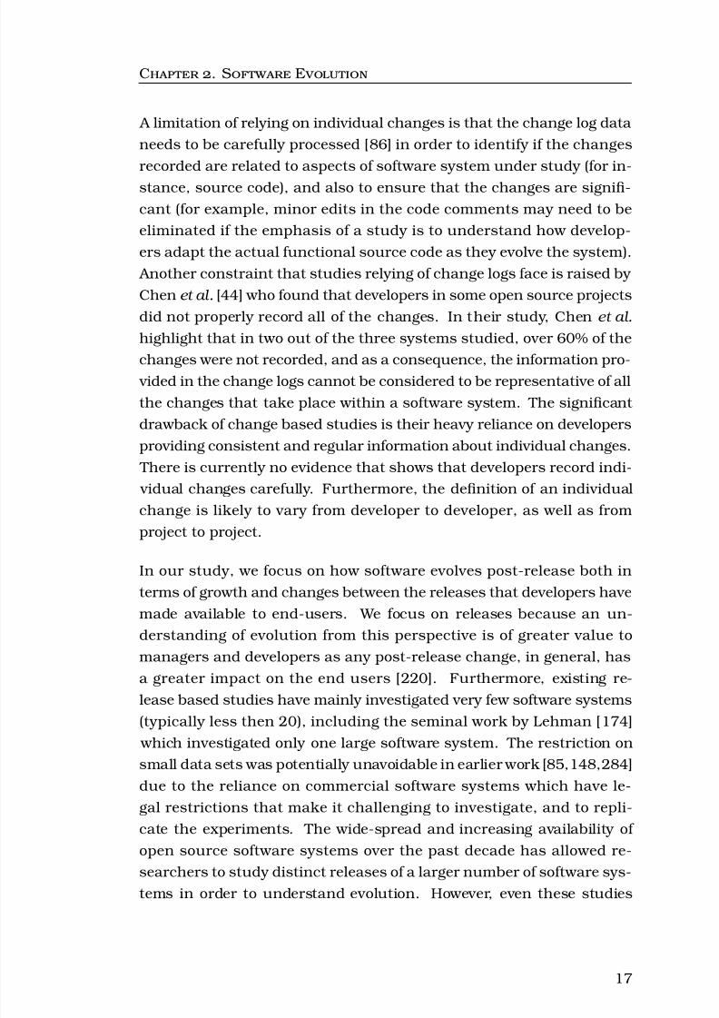
Within the context of software the term evolution has been used since
the 1960s to characterise growth dynamics. For example work by Halpern
[112] has shown how programming systems have evolved and Fry et.
11

8/8/2019 Rajesh Vasa -- PhD Thesis
http://slidepdf.com/reader/full/rajesh-vasa-phd-thesis 31/252
C . S E
Directed Selection(based on fitness)
Random Variation(Reproduction)
Process of Biological Evolution
Software System
Process of Software Evolution
Directed Adaptation(based on feedback/external pressures)
Population
Figure 2.1: The process of evolution.
al. [82] studied how database management systems evolve. The termin relation to how a software system changes started to appear in work
done by Couch [57]. Building on this foundation, Lehman [174], in his
seminal work argued that E-type software (application software used
in the real-world) due to their very use provide evolutionary pressures
that drive change. This argument was supported by the observation
that stakeholder requirements continually change, and in order to stay
useful, a software system must be adapted to ensure ongoing satisfac-
tion of the stakeholders. Unlike biological evolution which applies to a
population of organisms, the term software evolution is used within the
context of an individual software system. Similar to biological evolution,
the process of evolution in software is directed and feedback-driven to
ensure the software system is continuously adapted to satisfy the user’s
requirements. However, a key distinction is that in software evolution,
there is no random variation occurring within the software system (see
Figure 2.1) and the term “evolution” in the context of software implies
directed adaptation.
12

8/8/2019 Rajesh Vasa -- PhD Thesis
http://slidepdf.com/reader/full/rajesh-vasa-phd-thesis 32/252
C . S E
Although software evolution is typically used to imply a process of change
to an individual software system, it is also used within the context of
a product family [216], where the process involves a set of similar soft-
ware systems, akin to the concept of population in biology. Though in
both of these cases, there is a process of change, the object under study
is quite different - a single product versus an entire product family. Fur-
ther, the underlying drivers and mechanisms are also quite different.
When a product family is considered, evolution is a process with some
similarity to that in biological systems. For example, Nokia has a popu-
lation of mobile phones and they mine functionality from a range of their
models when creating new models [238]. In this scenario new phones
can be seen to descend from an ancestor and market driven mecha-nisms of selection of functionality, cross-breeding of functionality from
a number of models as well as intentional and random mutation where
new ideas are tried out.
In the context of this thesis, we take an approach similar to that used
by Lehman in this seminal work [174] and focus on the evolution of
individual software systems as they are adapted over time to satisfy
stakeholder requirements.
2.2 Software Evolution
Interestingly the term software evolution currently has no single widely
accepted definition [26] and the term is used to refer to both the process
of discrete, progressive, and incremental changes as well as the outcome
of this process [171]. In the first perspective, the focus is on evolution
as a verb (the process), and in the second perspective it is a noun (the
outcome) [171].
Lehman et al. [174] describe software evolution as the dynamic be-
haviour of programming systems as they are maintained and enhanced
over their life times . This description explicitly indicates evolution as
the observable outcome of the “maintenance” activity that causes the
changes, that is, the focus is on the outcome rather than the process.
13

8/8/2019 Rajesh Vasa -- PhD Thesis
http://slidepdf.com/reader/full/rajesh-vasa-phd-thesis 33/252
C . S E
Software maintenance which drives the software to change and evolve
as originally proposed by Swanson [267] and later updated in ISO-
14764 [126] involves the following mutually exclusive activities: (i) Cor-
rective work which is undertaken to rectify identified errors, (ii) Adaptive
work which is needed to ensure that the software can stay relevant and
useful to changing needs, (iii) Perfective work that is done to ensure it
meets new performance objectives as well as to ensure future growth,
and (iv) Preventive work that ensures that actively corrects potential
faults in the system, essentially as a risk mitigation activity. The main-
tenance activity, in general, is considered to take place after an initial
release has been developed and delivered [257].
Though the four key activities of maintenance as identified by ISO-
14764 [126] are a good starting point, Chapin [43] refines these into 12
orthogonal drivers that cause software evolution: evaluative, consul-
tive, training, updative, reformative, adaptive, performance, preventive,
groomative, enhancive, corrective, and reductive. Unlike the original
ISO-14764 classification which was based on intentions, Chapin’s ty-
pology is based on actual work undertaken as activities or processes,
and detected as changes or lack of in: (i) the software (executable),(ii) the properties of the software (captured from code), and (iii) the
customer-experienced functionality. In essence, Chapin et al. argue
that in a given software system, these are the three sources that can
change and evolve.
Within the context of this thesis, software evolution implies the measur-
able changes between releases made to the software as it is maintained
and enhanced over its life time . Software, the unit of change, includes
the executable as well as the source code. Our definition is a minor adaptation to the one proposed by Lehman [174], and reinforces the dis-
tinction between maintenance and evolution. It also explicitly focuses
on the outcome of the maintenance activity and changes that can be
measured from the software system using static analysis. That is, we
focus only on the set of changes that can be detected without executing
the software system, and without direct analysis of artifacts external to
the software system, for example, product documentation. Our study
focuses on the outcome from changes that are possible due to the fol-
14

8/8/2019 Rajesh Vasa -- PhD Thesis
http://slidepdf.com/reader/full/rajesh-vasa-phd-thesis 34/252
C . S E
lowing drivers (as per Chapin’s typology [43]): groomative, preventative,
performance, adaptive, enhancive, corrective and reductive.
Our definition of software evolution does not explicitly position it fromthe entire life-cycle (i.e. from concept till the time it is discontinued) of a
product perspective as suggested by Rajlich [230], but it ensures that as
long as there is a new release with measurable changes, then the soft-
ware is considered to be evolving. However, if there are changes made
via modifications to external configuration/data files, they will not be
within the scope of our definition. Similarly, we also ignore changes
made to the documentation, training material or other potential data
sources like the development plans. Alhough these data sources addadditional information, the most reliable source of changes to a software
system is the actual executable (and source code) itself. Hence in our
study of software evolution, we focus primarily on the actual artefact
and use other sources to provide supporting rationale, or explanation
for the changes.
Studies of Software Evolution
Studies into software evolution can be classified based on the primary
entities and attributes that are used in the analysis [25]. One perspec-
tive is to collect a set of measurements from distinct releases of a soft-
ware system and then analyze how these measures change over time in
order to understand evolution – these are referred to as release based
studies . The alternative perspective is to study evolution by analyzing
the individual changes that are made to a software system through-
out its life cycle – referred to as change based studies . These studiesconsider an individual change to be a specific change task, an action
arising from a change request, or a set of modifications made to the
components of a software system [25].
Release based studies are able to provide an insight into evolution from
a post-release maintenance perspective. That is, we can observe the
evolution of the releases of a software system that the stakeholders are
likely to deploy and use. The assumption made by these studies is that
15

8/8/2019 Rajesh Vasa -- PhD Thesis
http://slidepdf.com/reader/full/rajesh-vasa-phd-thesis 35/252
C . S E
developers will create a release of a software system once it is deemed to
be relatively stable and defect-free [254]. By focusing on how a sequence
of releases of a software system evolve, the release-based studies gain
knowledge about the dynamics of change between stable releases and
more importantly have the potential to identify releases with significant
changes (compared to a previous release). The assumption that devel-
opers formally release only a stable build allows release based studies
to identify patterns of evolution across multiple software systems (since
they compare what developers consider stable releases across different
systems) [254].
Change based studies, on the other hand, view evolution as the ag-gregate outcome of a number of individual changes over the entire life
cycle [25]. That is, they primarily analyze information generated during
the development of a release. Due to the nature of information that they
focus on, change based studies tend to provide an insight into the pro-
cess of evolution that is comparatively more developer centric. Although
change based studies can also be used to determine changes from the
end-user perspective, additional information about releases that have
been deployed for customers to use has to be taken into considerationduring analysis.
Though software evolution can be studied from both a release based
as well as the change based perspective, most of the studies in the lit-
erature have been based on an analysis of individual changes [139].
A recent survey paper by Kagdi et al. [139] reports on the result of
an investigation into the various approaches used for mining software
repositories in the context of software evolution. Kadgi et al. show that
most studies of evolution tend to rely on individual changes as recordedin the logs generated and maintained by configuration/defect manage-
ment systems (60 out of the 80 papers that they studied). Though a
specific reason for the preference towards studying these change logs is
not provided in the literature, it is potentially because the logs permit
an analysis of software systems independent of the programming lan-
guage, and the data is easily accessible directly from the tools typically
used by the development team (e.g. CVS logs).
16
8/8/2019 Rajesh Vasa -- PhD Thesis
http://slidepdf.com/reader/full/rajesh-vasa-phd-thesis 36/252
C . S E
A limitation of relying on individual changes is that the change log data
needs to be carefully processed [86] in order to identify if the changes
recorded are related to aspects of software system under study (for in-
stance, source code), and also to ensure that the changes are signifi-
cant (for example, minor edits in the code comments may need to be
eliminated if the emphasis of a study is to understand how develop-
ers adapt the actual functional source code as they evolve the system).
Another constraint that studies relying of change logs face is raised by
Chen et al. [44] who found that developers in some open source projects
did not properly record all of the changes. In their study, Chen et al.
highlight that in two out of the three systems studied, over 60% of the
changes were not recorded, and as a consequence, the information pro- vided in the change logs cannot be considered to be representative of all
the changes that take place within a software system. The significant
drawback of change based studies is their heavy reliance on developers
providing consistent and regular information about individual changes.
There is currently no evidence that shows that developers record indi-
vidual changes carefully. Furthermore, the definition of an individual
change is likely to vary from developer to developer, as well as from
project to project.
In our study, we focus on how software evolves post-release both in
terms of growth and changes between the releases that developers have
made available to end-users. We focus on releases because an un-
derstanding of evolution from this perspective is of greater value to
managers and developers as any post-release change, in general, has
a greater impact on the end users [220]. Furthermore, existing re-
lease based studies have mainly investigated very few software systems
(typically less then 20), including the seminal work by Lehman [174]
which investigated only one large software system. The restriction on
small data sets was potentially unavoidable in earlier work [85,148,284]
due to the reliance on commercial software systems which have le-
gal restrictions that make it challenging to investigate, and to repli-
cate the experiments. The wide-spread and increasing availability of
open source software systems over the past decade has allowed re-
searchers to study distinct releases of a larger number of software sys-
tems in order to understand evolution. However, even these studies
17

8/8/2019 Rajesh Vasa -- PhD Thesis
http://slidepdf.com/reader/full/rajesh-vasa-phd-thesis 37/252
C . S E
[59, 100, 101, 103, 127, 193, 204, 217, 239, 254, 277, 304, 310] focused
on a few popular and large software systems (for example, the Linux
operating system or the Eclipse IDE).
Interestingly, evolution studies that have consistently investigated many
different software systems (in a single study) are change based stud-
ies. Change based studies tend to use the revision logs generated and
maintained by the configuration management tools rather than col-
lecting data from individual releases in order to analyze the dynamics
within evolving software systems [25]. A few notable large change based
studies are Koch et al. [152, 153] who studied 8621 software systems,
Tabernero et al. [118] who investigated evolution in 3821 software sys-tems and Capiluppi et al. [39] who analysed 406 projects.
Given the small number of systems that are typically investigated in re-
lease based evolution studies, there is a need for a comparatively larger
longitudinal release based software evolution study to confirm findings
of previous studies still hold, to increase the generalizability of the find-
ings, and to improve the strength of the conclusions. Even though pre-
vious release based studies [59, 100, 101, 103, 127, 193, 204, 217, 239,
254, 277, 304, 310] have investigated a range of different software sys-
tems, a general limitation is that there has been no single study that
has attempted to analyze a significant set of software systems. Our
work fills this gap and involves a release based study of forty software
systems comprising 1057 releases. The focus on a comparatively larger
set of software systems adds to the existing body of knowledge since
our results have additional statistical strength than studies that inves-
tigated only a few software systems. Our data set selection criteria and
the method used to extract information is discussed in Chapter 3 andChapter 4, respectively.
2.3 The Laws of Software Evolution
The laws of software evolution are a set of empirically derived gener-
alisations that were originally proposed in a seminal work by Lehman
and Belady [168]. Five laws were initially defined [168] and later ex-
18

8/8/2019 Rajesh Vasa -- PhD Thesis
http://slidepdf.com/reader/full/rajesh-vasa-phd-thesis 38/252
C . S E
No. Name Statement1 Continuing
Change An E-type system must be continually adapted,else it becomes progressively less satisfactory
in use2 IncreasingComplexity
As an E-type system is changed its complexity increases and becomes more difficult to evolveunless work is done to maintain or reduce thecomplexity
3 Self Regulation
Global E-type system evolution is feedback reg-ulated
4 Conservationof Stability
The work rate of an organisation evolving anE-type software system tend to be constant over the operational lifetime of that system or phases of that lifetime
5 Conservationof Familiarity
In general, the incremental growth (growth ratetrend) of E-type systems is constrained by theneed to maintain familiarity
6 ContinuingGrowth
The functional capability of E-type systemsmust be continually enhanced to maintain user satisfaction over system lifetime
7 DecliningQuality
Unless rigorously adapted and evolved to takeinto account changes in the operational envi-ronment, the quality of an E-type system willappear to be declining
8 Feedback System
E-type evolution processes are multi-level,multi-loop, multi-agent feedback systems
Table 2.1: The Laws of Software Evolution [175]
tended into eight laws (See Table 2.1) [175]. These laws are based on
a number of observations of size and complexity growth in a large and
long lived software system. Lehman and his colleagues in their ini-
tial work discovered [168] and refined [171, 175] the laws of evolution
(which provide a broad description of what to expect), in part, from di-rect observations of system size growth (measured as number of mod-
ules) as well as by analysing the magnitude of changes to the modules.
The initial set of Five laws were based on the study of evolution of one
large mainframe software system. These five laws were later refined,
extended and supported by a series of case studies by Lehman and his
colleagues [171, 283, 284].
19

8/8/2019 Rajesh Vasa -- PhD Thesis
http://slidepdf.com/reader/full/rajesh-vasa-phd-thesis 39/252
C . S E
These empirical generalisations have been termed laws because they
capture and relate to mechanisms that are largely independent of tech-
nology and process detail. Essentially these laws are qualitative de-
scriptors of behaviour similar to laws from social science research and
are not as deterministic or specific as those identified in natural sci-
ences [198].
The Laws of Software Evolution (Table 2.1), state that regardless of do-
main, size, or complexity, real-world software systems evolve as they are
continually adapted, grow in size, become more complex, and require
additional resources to preserve and simplify their structure. In other
words, the laws suggest that as software systems evolve they becomeincreasingly harder to modify unless explicit steps are taken to improve
maintainability [175].
The laws broadly describe general characteristics of the natural incre-
mental transformations evolving software systems experience over time
and the way the laws have been described reflect the social context
within which software systems are constructed [198]. Furthermore,
these laws also suggest that at the global level the evolutionary be-
haviour is systemic, feedback driven and not under the direct control
of an individual developer [171].
The laws capture the key drivers and characteristics of software evo-
lution, are tightly interrelated, and capture both the change as well as
the context within which this change takes place [168, 170, 175]. The
first law (Continuing Change ) summarises the observation that soft-
ware will undergo regular and ongoing changes during its life-time in
order to stay useful to the users. These changes are driven by externalpressures, causing growth in the software system (captured as Con-
tinuing Growth by the sixth law) and in general, this increase in size
also causes a corresponding increase in the complexity of the software
structure (captured by the second law as Increasing Complexity ). Inter-
estingly, the process of evolution is triggered when the user perceives a
decrease in quality (captured as Declining Quality in the seventh law).
Additionally, the laws also state that the changes take place within an
environment that forces stability and a rate of change that permits the
20
8/8/2019 Rajesh Vasa -- PhD Thesis
http://slidepdf.com/reader/full/rajesh-vasa-phd-thesis 40/252
C . S E
organisation to keep up with the changes (captured by the fourth and
fifth laws of Conservation of Organisational Stability and Conservation
of Familiarity respectively). The laws suggest that in order to maintain
the stability and familiarity within certain boundaries, the evolution-
ary process is feedback regulated (third law – Self Regulation ), and that
the feedback takes place at multiple levels from a number of different
perspectives (eighth law of Feedback System ).
The Laws of Software Evolution are positioned as general laws [171,175]
even though there is support for the validity of only some of the laws [41,
59, 85, 171, 188, 192, 200]. However, there is increasing evidence [39,
100,101,103,119,120,127,153,217,239,277,306,310] to suggest that these laws are not applicable in many open source software systems and
hence have to be carefully interpreted (we elaborate on these studies in
the next section). A recent survey paper by Ramil et al. [192] studied
the literature and argues that there is consistent support for the first
law (Continuing Change) as well as the sixth law (Continuing Growth),
but no broad support exists for the other laws across different empirical
studies of open source software systems.
From a practical perspective, the applicability of the laws is limited by
their inability to provide direct quantitative measures or methods for in-
terpreting the changes that take place as software evolves [198]. Whilst
the laws of evolution continue to offer valuable insight into evolutionary
behaviour (effect), they do not completely explain the underlying drivers
or provide a behavioural model of change (the why) [169]. Despite many
studies into software evolution, a widely accepted cause and effect rela-
tionship has not yet been identified, potentially due to the large number
of inter-related variables involved and the intensely humanistic natureof software development that adds social aspects to the inherently com-
plex technical aspects [188, 192, 198].
In spite of their limitations, the laws of evolution have provided a consis-
tent reference point since their formulation for many studies of software
evolution, and therefore we investigate the validity and applicability of
these laws within our data set. Furthermore, our research approach
analyzes the distribution of growth and change (discussed in Chapter 5
21

8/8/2019 Rajesh Vasa -- PhD Thesis
http://slidepdf.com/reader/full/rajesh-vasa-phd-thesis 41/252
C . S E
and Chapter 6) rather than observe the overall growth trend in cer-
tain measures which is the technique employed by many earlier stud-
ies [39, 41, 59, 85, 100, 101, 103, 119, 120, 127, 153, 171, 175, 192, 200,
217, 239, 277, 306, 310] (discussed further in the next section – Sec-
tion 2.4). As a consequence our study can offer a different insight into
the laws, as well as the dynamics of change within open source software
systems.
2.4 Studies of Growth
The Laws of Software Evolution, as well as many studies over the last few decades have consistently shown that evolving software systems
tend to grow in size [188, 192]. But, what is the nature of this growth?
In this section we summarise the current understanding of the nature
of growth in evolving software systems. In particular, we focus heavily
on studies of growth in open source software systems as they are more
appropriate for the scope of this thesis.
In studies of software evolution, the observed growth dynamics are of interest as they can provide some insight into the underlying evolu-
tionary process [283]. In particular, it is interesting to know if growth
is smooth and consistent, or if a software system exhibits an erratic
pattern in its growth. For instance, managers can use this knowledge
to undertake a more detailed review of the project if development ef-
fort was consistent, but the resulting software size growth was erratic.
Although the observed changes do not directly reveal the underlying
cause, it can guide the review team by providing a better temporal per-
spective which can help them arrive at the likely drivers more efficiently.
Additionally, studies into growth dynamics also establish what can be
considered typical and hence provide a reference point for comparisons.
Lehman and his colleagues in their initial work [168] discovered and re-
fined [171,175] the laws of evolution (which provide a broad description
of the dynamics of software evolution), in part, from direct observations
of size growth in long lived commercial software systems.
22

8/8/2019 Rajesh Vasa -- PhD Thesis
http://slidepdf.com/reader/full/rajesh-vasa-phd-thesis 42/252
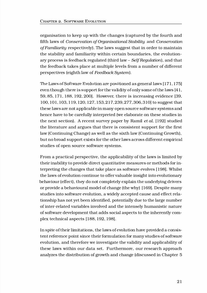
C . S E
time
s i z e
time
s i z e
time
s i z e
Sub-Linear Growth Super-Linear Growth Linear Growth
Figure 2.2: The different types of growth rates observed in evolvingsoftware systems.
Growth rate
The laws of evolution state that software will grow as it is adapted to
meet the changing user needs. However, what is the typical growth
rate that we can expect to see in a software system? A consistent and
interesting observation captured in early studies [85,168,175,283] into
software evolution was that the typical rate of growth is sub-linear (see
Figure 2.2). That is, the rate of growth decreases over time. The laws of
software evolution suggest that this is to be expected in evolving soft-
ware since complexity increases (second law), and average effort is con-sistent (Fourth Law). The argument that is extended to support the
sub-linear growth expectation is that in evolving software, the increas-
ing complexity forces developers to allocate some of the development
effort into managing complexity rather than towards adding new func-
tionality [283] resulting in a sub-linear growth rate.
A model that captures this relationship between complexity and growth
rate is Turski’s Inverse Square Model [283, 284]. Turski’s model (see
Equation 2.4.1) is built around the assumption that the system size
growth as measured in terms of number of source modules is inversely
proportional to its complexity (measured as a square of the size to cap-
ture the number of intermodule interaction patterns) and has been
shown to fit the data for a large long-lived software system [283].
23

8/8/2019 Rajesh Vasa -- PhD Thesis
http://slidepdf.com/reader/full/rajesh-vasa-phd-thesis 43/252
C . S E
Turski’s Inverse Square model [283] is formulated with system size
S at release i (Si) and constant effort E. Complexity of software is
the square of the size at previous version (S2
i−1).
Si =E
S2i−1
+ Si−1 (2.4.1)
Beyond the work by Turski [283, 284], the sub-linear growth rate ob-
servation is also supported by a number of different case studies [41,
59, 85, 171, 175, 188, 192, 200, 217] that built models based on regres-
sion techniques. The increasing availability and acceptance of Open
Source Software Systems has allowed researchers to undertake com-paratively larger studies in order to understand growth as well as other
aspects of evolution [39, 100, 103, 127, 217, 306]. Interestingly, it is
these studies that have initially provided a range of conflicting results,
some studies [17, 129, 153] found that growth typically tends to be
sub-linear supporting the appropriateness of Lehman’s laws, but oth-
ers [101, 119, 120, 127, 153, 239] have observed linear as well as super-
linear growth rates suggesting that the growth expectations implied by
Lehman’s laws of evolution are not universal.
Godfrey and his colleagues [101] were one of the first to question the
validity of Lehman’s laws in the context of Open Source Software Sys-
tems. In their study they observed growth to be super-linear in certain
sub-systems of Linux (specifically the driver sub-system in their study),
suggesting that the increasing complexity and sub-linear growth rate
expectation of Lehman’s laws do not universally hold. This observation
of super-linearity was later confirmed by Succi et al. [264], González-
Barahona et al. [105, 106] and more recently by Israeili et al. [127].
In contrast to these multiple findings on super-linear growth rates,
Izurieta et al. [129] found no evidence of super linear growth rate in
FreeBSD and the Linux kernels. Godfrey et al. [100] found that Fetch-
mail (e-mail retrieval and forwarding system), X-Windows (a Window
manager) and the gcc compiler exhibit near linear growth while the Pine
e-mail client had a sub-linear growth rate. Additional evidence from a
study by Paulson et al. [217] suggests that the Linux kernel, Apache
24
8/8/2019 Rajesh Vasa -- PhD Thesis
http://slidepdf.com/reader/full/rajesh-vasa-phd-thesis 44/252
C . S E
Web server and gcc compiler all showed only linear growth. Robles et
al. [239] analyzed 18 different open source software systems and found
that sub-linear and linear growth rates to be the dominant trend with
only two systems (Linux and KDE) fitting a super-linear growth trend.
Mens et al. [192] in a study of the evolution of the Eclipse IDE observed
super-linear growth in the number of plug-ins, while the core platform
exhibited a linear growth rate. Koch [152], in an extensive change based
study of over 4000 different software systems mined from Sourceforge (a
popular open source software repository), found linear and sub-linear
growth rates to be common, while only a few systems exhibited super-
linear growth rate. Though, Koch et al. undertook a change based
study by analysing the source code control logs, they reconstruct sizemeasures in order to analyze the growth rates. More recently, Thomas
et al. [277] investigated the rate of growth in Linux kernel and found a
linear growth rate.
Researchers [101, 127, 153, 192, 200] that have observed the super-
linear growth rate argue that the underlying structure and organisa-
tion of a system has an impact on the evolutionary growth potential
and that modular architectures can support super-linear growth rates. They suggest that these modular architectures can support an increas-
ing number of developers, allowing them to make contributions in par-
allel without a corresponding amplification of the communication over-
head [153].
From an alternate perspective, in systems with a plug-in architectural
style, evolutionary growth can be seen as adding volumetric complex-
ity without a corresponding increase in the cognitive complexity [101].
This is the case because developers do not need to gain an understand-ing of all of the plug-ins in the system, rather they need to understand
the core framework and the plug-in interface in order to add new func-
tionality. For instance, in the case of Linux, the super-linear growth was
attributed to a rapid growth in the number of device drivers [101], most
of which tend to adhere to a standard and relatively stable functional
interface, allowing multiple development teams to contribute without
increasing the communication overhead and more importantly without
adding defects directly into the rest of the system. Similarly, the expo-
25

8/8/2019 Rajesh Vasa -- PhD Thesis
http://slidepdf.com/reader/full/rajesh-vasa-phd-thesis 45/252
C . S E
nential growth in the number of plug-ins for the Eclipse platform [192]
is similar to that of the driver sub-system in Linux and shows that cer-
tain architectural styles can allow the overall software systems to grow
at super-linear rates, suggesting limitations to Lehman’s laws.
Studies that found super-linear growth rates [101, 119, 120, 127, 153,
239] show that it is possible to manage the increase in volumetric com-
plexity and the consequent structural complexity. The implication of
these studies is that certain architectural choices made early in the
life cycle can have an impact on the growth rate, and a certain level of
structural complexity can be sustained without a corresponding invest-
ment of development effort (in contrast to the expectations of the lawsof software evolution).
A consistent method that is generally applied by earlier studies of growth
has been to observe how certain system wide measures change over
time (for example, Number of modules). These observations have then
typically been interpreted within the context of Lehman’s laws of evo-
lution in order to understand growth dynamics within evolving soft-
ware systems. Though these previous studies have improved our un-
derstanding of how software evolves, there is limited knowledge with
respect to how this growth is distributed among the various abstrac-
tions of a software system.
An early study that has provided some data about the distribution of
growth is the one undertaken by Gall et al. [85] that suggests that differ-
ent modules grow at different rates. This observation is also confirmed
by Barry et al. [17]. Although these studies highlight that growth rates
can differ across modules, they do not discuss in depth how the growthis distributed and what the impact of this distribution is on the over-
all evolution of the software that they study. More recently, Israeli et
al. [127] investigated the Linux kernel and identified that average com-
plexity is decreasing. The interesting aspect of the study by Israeli et al.
was that they note that the reduction of the average complexity was a re-
sult of developers adding more functions with lower relative complexity.
However, all of these studies have focused on individual systems and on
a small set of metrics, and hence there is a gap in our understanding
26

8/8/2019 Rajesh Vasa -- PhD Thesis
http://slidepdf.com/reader/full/rajesh-vasa-phd-thesis 46/252
C . S E
y = 0.0001x2 + 0.1072x + 213.29
R² = 0.97821
y = ‐0.0002x2 + 0.3909x + 174.69
R² = 0.9659
y = ‐0.0009x2 + 3.4153x ‐ 2516.7
R² = 0.9968
0
100
200
300
400
500
600
700
800
900
1000
0 500 1000 1500 2000 2500
S i z e ( N u m b e r o f C l a s s e s )
Age (Days)
Version 1.0.x (Sub‐Linear)
Versions 1.1.x to 1.6.x (Sub‐Linear)
All versions (Super‐Linear)
Figure 2.3: Illustration of the segmented growth in the Groovy lan-guage compiler. The overall growth rate appears to be super-linear, with two distinct sub-linear segments.
of how different measures are distributed and if a general pattern ex-
ists in terms of how growth is distributed across a larger set of software
systems.
Segmented Growth
The common theme in studies of growth [101, 127, 152, 153, 192, 217,
239] is that they focus on the growth over the entire evolution history
and as a consequence attach only a single growth rate to software sys-
tems. That is, they tend to classify the size growth of a system to be
one of the following: sub-linear, linear, or super-linear. However, when
a more fine-grained analysis was performed, software systems under-going evolution have been shown to exhibit a segmented and uneven
growth pattern. That is, the software system can grow at different rates
at different time periods [6,120,123,175,256,305], and also that some
modules can grow much faster than others [17, 85]. This segmented
growth pattern is illustrated in Figure 2.3. The data in the figure is
from one of the software systems that we analyse in our study and
highlights the need for analyzing growth from different perspectives.
27
8/8/2019 Rajesh Vasa -- PhD Thesis
http://slidepdf.com/reader/full/rajesh-vasa-phd-thesis 47/252
C . S E
The observation of segmented growth has been used to suggest that
developers periodically restructure and reorganise the code base po-
tentially causing a temporary reduction in size and complexity followed
by a period of renewed growth [175]. An example of this segmented
growth has been captured by Capiluppi et al. [38 – 41] in a sequence of
studies. They presented evidence that shows that open source software
systems tend to have segmented growth where each segment may have
a different growth rate. For instance, Capiluppi et al. note that Gaim
(an internet chat software that was investigated in their study) grows at
a super-linear rate early in its life cycle, with a large gap in development
followed by a linear growth rate.
The segmented growth pattern has also been confirmed by Smith et
al. [256] and by Wu et al. [304, 305]. Smith et al. [256] studied 25 open
source systems developed in C/C++ and showed that growth rates are
not consistent during the evolution of a software system and that they
can change. More recently, Wu et al. [304, 305] presented evidence of a
punctuated growth in open source software system based on a study of
3 systems (including Linux). Wu et al. observed that developers work
in periodic bursts of activity, where intensive effort goes into creating a major release followed by a less active period where minor defects are
corrected. Additionally, work done by Hsi et al. [123] has also shown
how the evolutionary drivers result in asymmetric and clumpy growth.
Summary
Studies of software evolution that have investigated the phenomenon
of growth have shown that the rate of growth can be super-linear, lin-ear or sub-linear. Furthermore, since this growth has been shown to
be segmented, there are limitations in the value offered by an under-
standing of the overall growth rate. Additionally, the lack of consis-
tency with respect to the observed growth rate in the studies of evolu-
tion [101, 127, 152, 153, 192, 217, 239] shows that there are limitations
within the explanation of the dynamics as postulated by the laws of
software evolution [175]. Specifically, there is evidence to suggest that
the complexity that arises due to evolution does not necessarily create
28

8/8/2019 Rajesh Vasa -- PhD Thesis
http://slidepdf.com/reader/full/rajesh-vasa-phd-thesis 48/252
C . S E
a drag on the rate of growth [101]. Another aspect is that the studies
identifying linear and super-linear growth rates show that the parame-
ters considered in simple growth models (like Turski’s [283,284], or by
models developed using regression techniques) are not sufficient when
attempting to model and understand growth. That is, though there is
some relationship between complexity and growth, there may be other
aspects that influence the growth of a software system.
Current models and methods of understanding of growth in evolving
software [118, 119, 127, 153, 168, 175, 200, 217, 239, 277, 284, 305, 310]
have allowed for inferences to be drawn about certain attributes of
the software system, for instance, regarding the architecture [100, 101,127, 153, 192, 200, 290, 294], complexity and its impact on the effort
[118, 168, 284]. However, an inherent limitation of these models is that
they do not provide any direct insight into where growth takes place. In
particular, we cannot assess the impact of evolution on the underlying
distribution of size and complexity among the various classes. Such
an analysis is needed in order to answer questions such as “do devel-
opers tend to evenly distribute complexity as systems get bigger?” , and
“do large and complex classes get bigger over time?” . These are ques-tions of more than passing interest since by understanding what typical
and successful software evolution looks like, we can identify anomalous
situations and take action earlier than might otherwise be possible. In-
formation gained from an analysis of the distribution of growth will also
show if there are consistent boundaries within which a software design
structure exists.
In particular a key gap in our understanding of growth arises because
previous studies have, in general, analyzed the changes to the aggregatemeasures (for example, the growth of total SLOC, or the total number
of classes) rather than how these measures are distributed within the
abstractions of a software system. This additional detail is necessary
in order to gain an insight into the decisions that developers make.
That is, when developers add, modify and extend existing classes, do
they gradually centralise functionality and complexity, or does this pro-
cess spread out the functionality and complexity across classes? This
knowledge of the typical patterns of growth and its distributions can be
29
8/8/2019 Rajesh Vasa -- PhD Thesis
http://slidepdf.com/reader/full/rajesh-vasa-phd-thesis 49/252
C . S E
used to guide development teams to identify abnormal growth patterns.
Further, we can also verify if developers follow what are considered good
software engineering practice and avoid god classes [237] as software
evolves. This form of analysis is also helpful in early identification of
abnormal and unusual changes. This is necessary because research
into software reliability shows us that structurally complex parts of the
software tend to contain a higher rate of defects [20, 205, 281, 317] and
early identification of parts that are gaining in complexity will allow us
to take corrective actions sooner.
In our study we aim to close these gap in our understanding and ob-
serve evolution from a different perspective. Rather than use globalsize growth models to infer support for laws and understand the na-
ture of evolution, we study software evolution by observing how the
distribution of size and complexity changes over time. More specifically,
we undertake a longitudinal study that constructs probability density
functions of different metrics collected from the software systems, and
builds a descriptive model of evolution by observing how these metric
distributions change over time.
2.5 Studies of Change
It is a widely accepted that software systems that are in active use need
to be changed at some or many stages of its life in order to stay use-
ful [175, 188, 192]. Given that change is the one inherent constant of
an active and used software system, the key to a successful software
evolution approach lies, however, not only in adapting a system to sup-
port the new requirements [87], but also in understanding the nature
and the dynamics of change. Managing and reducing the costs and
risks of changes to software that arise as part of the maintenance pro-
cess are important goals for both research and the practice of software
engineering [25, 220].
The laws of software evolution, as well as a number of other studies,
have consistently suggested that evolving software will grow and un-
dergo change as it is adapted [175,188,192,293]. Since software growth
30

8/8/2019 Rajesh Vasa -- PhD Thesis
http://slidepdf.com/reader/full/rajesh-vasa-phd-thesis 50/252
C . S E
is dependent on change, a proper understanding of the nature and type
of changes that a software system undergoes is important to under-
stand the growth dynamics. For instance, the growth can be caused by
developers adding new abstractions, removing existing code, or modi-
fying some existing abstractions. Furthermore, studies of change can
help address questions such as – Are there any common and recurring
patterns of changes? Do developers tend to grow software by creat-
ing new abstractions?, or Do they prefer to modify and extend existing
abstractions?, and Do certain attributes make a class more change-
prone?. Knowledge gained from these studies of change help us un-
derstand growth better [102], improve development plans by providing
information about the typical patterns and impact of change [281], andidentify and inform developers of the changes that they made in a spe-
cific time interval to help them reflect on the development process bet-
ter.
Detecting Change
The first step in understanding change is to identify the unit of change ,
specifically, the entity that is undergoing change [17]. In this thesis, we take a class to be the unit of change. We study classes since they
are the primary organisational abstractions in object-oriented software
systems [185, 186]. A class contains both data as well as methods and
is the natural abstraction that developers use when designing, con-
structing and modifying an object oriented software system. Although,
change can be studied at a lower level of abstractions such as a method,
within object-oriented software systems, a method is considered to be a
part of a class and hence any change to methods are better understood within the context of a class. Similarly, focusing on a higher-level ab-
straction such as a package or a component provides a coarse-grained
view of change than can be obtained by observing changes in classes.
The next step in understanding change requires the detection of change
in a class. There are two approaches that are typically used to detect
change in a class. The first, and more widely used method is to identify
change by analysing transaction logs (e.g. CVS logs, issue logs) created
31

8/8/2019 Rajesh Vasa -- PhD Thesis
http://slidepdf.com/reader/full/rajesh-vasa-phd-thesis 51/252
C . S E
during the development of a specific release [25]. This is the analy-
sis technique preferred by change based studies (as discussed in Sec-
tion 2.2). Though this approach is widely used in the literature [138],
there are significant limitations to this method of detecting change. The
transaction logs that are used as input for detecting change do not di-
rectly record the nature of change. Specifically, they do not record if the
modification altered the functional semantics of the program, or if the
change was purely cosmetic [80]. For instance, widely used source code
control systems such as CVS and SVN record changes by string compar-
ison between two text files and tend to identify the lines added, removed
and modified. However, these tools do not check if the change impacts
the actual semantics of the program. That is, these tools treat thefollowing change actions identically – comment addition, source code
reformatting, and removing a method from a class. This inability of the
current generation of popular tools of recording the type of change is a
significant limitation if a study purely relies on data generated by these
tools to detect change. The limitation arises because changes to the
functional aspects of a class have a greater impact in maintenance as
they have the potential to impact other classes [281], and as a conse-
quence have a higher risk profile.
The second approach to detecting change analyses the actual class (or a
program file) at two different points in time in order to determine if it has
changed. This approach, referred to as origin analysis in the literature
[102,282] is comparatively more complex, but provides a more accurate
reflection of the changes since there is no reliance on reconstructing
change information by analysing an external transaction log. Detecting
change between two releases of a class has been an area of study for
many years [242,282] and different methods to assist in the detection of
the change have been developed [5,22,72,80,135,143,155,243,294]. In
this thesis, we detect changes by analysing classes in two consecutive
releases as it enables us to focus on changes to the functional aspects
of a program. A more detailed discussion of these techniques, their
strengths and limitations, as well as our own method for detecting the
change is presented in Chapter 6.
32

8/8/2019 Rajesh Vasa -- PhD Thesis
http://slidepdf.com/reader/full/rajesh-vasa-phd-thesis 52/252
C . S E
Dimensions of Change
Change is defined1 as a process of transformation — to make the form
different from what it is . Some of the earliest studies that attempted to
investigate and understand the nature of change were undertaken by
Lehman et al. [168, 175] as part of the work that developed the Laws of
Software Evolution. Lehman et al. were able to establish that existing
software was being adapted based on direct observation of size growth,
and confirmation from the development team that the software was
being adapted to meet changing requirements. Based on the work by
Lehman et al., Gall et al. [85] observed change by measuring the number
of program files that were added, removed and modified in each release by analysing 20 releases of a single commercial software system. In this
study, Gall et al. showed that some modules changed more than others
and also that the rate of change, in general, decreased over time. More
recent studies have focused on observing changes by measuring the
number of functions that were modified, and also by observing how the
complexity of functions changed over time [217, 291, 310]. A common
finding in these studies of change is that they confirm the applicability
of the First Law of Software Evolution – Continuing Change . A recent survey paper by Ramil et al. [192] that summarises empirical studies
of evolution within the context of open source software evolution also
suggests that there is consistent support for the first law.
Early work of Lehman et al., as well as following studies into software
evolution (as discussed in previous sections) have consistently found
that software is adapted as it evolves. However, they have not focused
on a more detailed analysis of the various dimensions of change. A
method to understand change more effectively was proposed by Barry et al. [17] where they argue that volatility within software has three
distinct dimensions from which it can be studied: amplitude (size of
change), periodicity (frequency of change), and dispersion (consistency
of change). Amplitude measures the size of modification and a number
of different approaches can be applied to determine this amplitude. An
example of a method used to determine the amplitude of change in a
file (at two instances in time) can be measured as the sum of the lines
1Oxford American Dictionary, 2005
33

8/8/2019 Rajesh Vasa -- PhD Thesis
http://slidepdf.com/reader/full/rajesh-vasa-phd-thesis 53/252
C . S E
added, removed and modified [85, 217]. Periodicity measures the reg-
ularity at with a system or an abstraction is modified. For instance,
this measure is required to determine how often a file is modified over
the evolution history. The expectation is that if a large part of the code
base is modified frequently, then the software is highly volatile and may
require corrective action. Finally, the measure of dispersion aims to
identify if there is a consistent pattern to the change. This measure
is motivated by the assumption that consistency allows managers to
anticipate how much of the code base may change in the next version
and hence can allocate resources appropriately. The dispersion mea-
sure can be applied to determine the consistency of the size of change,
as well as the consistency in the frequency of change. In this thesis, we study change against these three dimensions. A discussion our ap-
proach to compute change against these three dimensions is presented
in Chapter 6.
Studies of change that investigate these dimensions are able to provide
us with a baseline on what to expect in evolving software. Specifically,
we can identify periods of normal and abnormal change. Though an
understanding of these dimensions of change is useful [17], we foundcomparatively few studies in the literature that have focused on a quan-
titative analysis of these dimensions of change. Furthermore, most
studies investigated only a few software systems (typically under 10),
impacting on the strength of their findings.
An early study that presents observations from an investigation of the
frequency of change was undertaken by Kemerer et al. [147] who stud-
ied the profile of software maintenance in five business systems at the
granularity of modules. They concluded that very few modules changefrequently, and later extended this study by identifying that the mod-
ules that did change can be considered to be strategic [148] (in terms of
business functionality offered). Both of these studies inferred change
by analysing defect logs generated during the development of a com-
mercial non-object oriented software system. This study was not able
to establish the typical size of change, or the consistency of the change.
34

8/8/2019 Rajesh Vasa -- PhD Thesis
http://slidepdf.com/reader/full/rajesh-vasa-phd-thesis 54/252
C . S E
More recent work by Purushothaman et al. [228] has provided some
insight into the size of change. Purushotham et al., based on an anal-
ysis of the source code revision control system logs conclude that most
of the changes are very small based on the observation that 95% of
the changes required a modification of less than 50 lines of code. A key
weakness of this study is that it was based on a single large commercial
software system, and hence lacks sufficient generalizability. Another
study that investigated the size of change was undertaken by Mockus
et al. [201] who observed that the size of change was very small for
defect corrections. The study by Mockus et al. however does not pro-
vide any further insight into the dimensions of change beyond defect
corrections.
Wu et al. [304, 305] in a release-based study investigated the nature of
change in 3 open-source software systems. They found that projects
alternate between periods of localised small incremental changes and
periods of deep architectural changes (which impacted a large number
of modules). The studies by Wu et al. focused on a comparatively small
data set, and investigated only architectural changes by analysing how
incoming and outgoing dependencies for each object file change over time.
Anton et al. [3, 4] investigated change in the set of functionality offered
by the telephone network to end-users over a 50 year period. Antonet al.
showed that different change drivers apply at different times and that
functional evolution takes place in discrete bursts followed by gradual
enhancement giving rise to a “punctuated equilibrium” pattern [14]. In-
terestingly, this is the pattern that Wu et al. also identified in their work
even though the granularity and perspectives of these two studies are vastly different. Although the study by Anton et al. is interesting, their
findings are helpful to review and understand long-term strategy rather
than in directly helping developers understand the nature of changes
within the software system at a local level over a relatively shorter time
interval.
A different perspective to understanding dimensions of change in the
context of object-oriented software systems has been driven by researchers
35

8/8/2019 Rajesh Vasa -- PhD Thesis
http://slidepdf.com/reader/full/rajesh-vasa-phd-thesis 55/252
C . S E
that focused on visualising software evolution [65, 95]. A simple, yet
powerful method is the Evolution Matrix proposed by Lanza et al. [163]
as a means to visualize the evolution, with the emphasis on revealing
patterns of change. This method has the advantage of being able to
provide a good overview for developers when they retrospectively audit
the evolution of a project in order to gain a better understanding of the
history and make improvements for the future. More recent work in evo-
lution visualization [1, 164, 298] has aimed at highlighting changes to
the design structure of a software system based on thresholds for met-
ric values at various levels of abstraction (for instance, class or package
level). Interestingly, research into visualization of evolution has focused
on improving the quality and quantity of information that is commu-nicated to the users. However, these visualizations can be improved if
they have additional statistical information about the change patterns.
Change-prone Classes and Co-Change
In the context of object-oriented software systems, the aspect of change
that has been investigated in considerable depth within the literature
is identification of attributes that make a class change-prone, and de-tecting groups of classes that change together. The motivation for un-
derstanding change-prone classes is to improve the design of a software
system, and minimise the need for change since modifications are con-
sidered to be risky and potentially defect inducing [205]. These stud-
ies into change-prone classes have identified some common aspects
and have provided consistent evidence showing that structurally com-
plex and large classes tend to undergo more changes [20,28,31,63,130,
177, 213, 214, 261, 266, 314, 318], and classes that changed recently are likely to undergo modifications in the near future [92, 93]. Stud-
ies that focused on change-prone classes do have some weaknesses.
These studies have, in general, investigated only a few software systems
and different studies have used slightly different methods for detect-
ing change. However, given the recurring confirmation across multiple
studies, the expectation that structurally complex classes will undergo
more changes can be considered to be a strong possibility. Although
there is considerable agreement that complexity and change are related,
36

8/8/2019 Rajesh Vasa -- PhD Thesis
http://slidepdf.com/reader/full/rajesh-vasa-phd-thesis 56/252
C . S E
a larger scale study can help improve the strength of this expectation
and can provide a more robust model that captures the relationship
between complexity and change.
Interestingly, these studies of change-prone classes have measured com-
plexity within an individual class, typically using complexity measures
proposed by Chidamber and Kemerer [46], or variations of these mea-
sures [116, 165]. For example, a commonly used measure of class
complexity is the WMC (Weighted Method Count) with the McCabe Cy-
clomatic Complexity measure [190] used as the weight. Though the
complexity of a class has been used to determine change-proneness,
there is a gap in our understanding of the relationship between change-proneness and a class gaining new dependents. This aspect has not
been properly investigated since the measures of a class complexity fo-
cus mainly on the set of classes that a particular class depends upon,
rather than the set of classes that it provides services to. A recent
change-based study by Geipel et al. [89], however, does present some
evidence of a relationship between class dependencies and change prop-
agation. Similarly, Sangal et al. [245] also show that a high concentra-
tion of dependencies acts as a propagator of change. Although, Giepelet al. and Sangal et al. suggest that a class with a high concentration
of dependencies will propagate change, we do not fully understand the
likelihood of change in a class that acts as a service provider as it gains
new dependencies.
Another arc in the study of change has been the area of understand-
ing co-change, where the expectation is that certain groups of classes
or modules change together [85] because developers tend to group and
construct related features together. This expectation is supported by research undertaken by Hassan and Holt who analyzed many Open
Source projects and concluded that historical co-change is a better
predictor of change propagation [113]. This observation is also sup-
ported by Zimmerman et al. [319, 320] which led to the development
of tools [315] that can guide developers to consider a group of classes
when they modify one class. These studies into co-change have been
instrumental in developing tools that can help developers consider the
impact of a change by exposing a wider ripple impact than is visible to
37

8/8/2019 Rajesh Vasa -- PhD Thesis
http://slidepdf.com/reader/full/rajesh-vasa-phd-thesis 57/252
C . S E
the compiler (via a static dependency analysis). However, these studies
have relied on an analysis of revision logs and hence provide an under-
standing of changes during the construction of a release. There is still
a gap in our understanding of post-release change, specifically in terms
of statistical properties against the various dimensions of change.
Summary
Studies of change have a general theme. They have primarily used logs
generated by the tools used in software development [138], and the typi-
cal focus has been mostly on establishing attributes within classes that
make them change-prone [20, 28, 31, 63, 130, 177, 213, 214, 261, 266,
314, 318]. Also, these studies have arrived at their conclusions us-
ing relatively small number of software systems, and the emphasis has
been on understanding fine-grained changes during the construction
of a release rather than post-release.
There is currently a gap in our understanding of post-release changes
in object-oriented software systems, specifically since existing studies
capture only broad patterns of change based on an analysis of smalldata sets [4, 305]. Although previous studies suggest that change fol-
lows a punctuated equilibrium pattern with the size of change being
small, they do not provide a statistical model of change. For instance,
we currently do not have models that can help estimate the proportion
of classes that are likely to be modified if the developers plan on adding
a set of new classes. Additionally, developers also need to know where
they can expect the changes within the context of their software sys-
tem, and the magnitude of these modifications in order to take proac-tive steps and mitigate any potential risks arising from these changes.
This gap can be addressed by creating descriptive statistical models of
change as these models can assist in developing tools that highlight
and monitor evolution prone parts of a system as well as support ef-
fort estimation activities. An additional gap in current studies is that,
in general, they do not establish thresholds that can be used to flag
potentially significant and systemic changes within an object-oriented
software system.
38

8/8/2019 Rajesh Vasa -- PhD Thesis
http://slidepdf.com/reader/full/rajesh-vasa-phd-thesis 58/252
C . S E
In our study of change we aim to address these gaps by focusing our
effort towards developing statistical models that can help establish nor-
mal and unusual patterns of change. We also use these models to un-
derstand better how evolving software systems grow, in particular, we
can identify if growth is achieved by creating new abstractions, or if
existing abstractions are modified and extended.
2.6 Research Questions
Evolution in software has been a field that has been investigated over
the past few decades, with a heavier emphasis on object-oriented soft- ware systems over the past decade. These studies consistently establish
that evolution causes growth as software is adapted to meet changing
user requirements. In this chapter, we presented a summary of the key
studies related to our focus areas – growth and change. A common as-
pect across much of the previous work is that the studies have focused
on a few software systems, used different input data sources in their
investigation, and the abstractions under study have not been consis-
tent across these studies. Furthermore, the current understanding of growth has been established primarily by studies of aggregate system
level size and complexity growth rather than by how this growth is dis-
tributed across the various parts of the software system. The focus
of studies on change has been on identification of attributes that can
make an entity change-prone, with a significant emphasis on changes
during the construction of a release rather than post-release.
In order to address the gaps identified, we framed a set of research
questions related to growth and change. As indicated earlier, our in-
tention is to study growth in terms of how it is distributed across the
various classes within an object-oriented software system. We investi-
gate change as a means to better understand growth as well as to how
and where the maintenance effort is focused by the developers as they
modify, add and remove classes.
39

8/8/2019 Rajesh Vasa -- PhD Thesis
http://slidepdf.com/reader/full/rajesh-vasa-phd-thesis 59/252
C . S E
The questions related to growth that we address in this thesis are:
• What is the nature of distribution of size and complexity mea-
sures?
• How does the profile and shape of this distribution change as soft-
ware systems evolve?
• Do large and complex classes become bigger and more complex as
software systems evolve?
The questions related to change that we address in this thesis are:
• What is the likelihood that a class will change from a given version
to the next?
• How is modification frequency distributed for classes that change?
• What is the distribution of the size of change? Are most modifica-
tions minor adjustments, or substantive modifications?
• Does complexity make a class change-prone?
Our study address the gaps in the current literature by investigating
the evolution in forty non-trivial object-oriented Java software systems.
The larger data set, as well as the consistent measures that we ap-
ply across 1057 releases under investigation in our study increases
the strength of our conclusions. We analyse growth across a range
of different measures and focus on how growth is distributed across
the various classes. Furthermore, our study focuses on understanding
post-release changes which have a relatively higher risk profile.
The next chapter (Chapter 3) presents the input data set, our selection
criteria and the aspects that we investigate. Chapter 4 (Measuring Java
Software) follows with a discussion of the metric extraction process and
defines the metrics we collect from the Java software systems. The key
findings of this thesis are presented in Chapter 5 (Growth Dynamics)
and Chapter 6 (Change Dynamics). We discuss the implications arising
from our findings in Chapter 7 and conclude in Chapter 8.
40

8/8/2019 Rajesh Vasa -- PhD Thesis
http://slidepdf.com/reader/full/rajesh-vasa-phd-thesis 60/252
Chapter 3
Data Selection Methodology
Empirical research by its very nature relies heavily on quantitative infor-
mation. In our study, we extract information from a number of different
Open Source Software Systems. This chapter provides an overview of
the various sources of information that can be used to study evolution,
the Open Source Software Systems that we selected, and the criteria
used to select the software systems.
3.1 Evolution History
Research into software evolution relies on historical information. When
information is extracted from various data sources (for example, source
code, project plans, change logs etc.) of a software project over time, we
obtain the evolution history of a software system. Broadly classified,
there are three types of evolution histories (see Table 3.1): (i) the re- lease history, (ii) the revision history, and the (iii) the project history.
The release history contains the software artifacts that are released at
regular intervals in the project. The revision history is composed of
the version control logs and issue/defect records. The project history is
made up of the messages (e.g. email, chat logs), project documentation
as well as process information.
The software artifacts from the release history (specifically binaries and
source files) offer a direct evolutionary view into the size, structure and
41

8/8/2019 Rajesh Vasa -- PhD Thesis
http://slidepdf.com/reader/full/rajesh-vasa-phd-thesis 61/252
C . D S M
History Description
Release History Source code, binaries, release notes, and releasedocumentation
Revision History Version control logs, issue/defect records, Modifi-cation history of documentation, Wiki logs
Project History Messages (email, Instant message logs), Project documentation (plans, methodology, process)
Table 3.1: The different types of histories that typically provide input data for studies into software evolution.
composition of the actual software system. The other categories of in-
formation tend to provide a supporting, indirect view and can help fill in
the gaps in understanding the evolution of a software system. However,the information derived from the revision history and project history is
reliable only if the development team was disciplined enough to record
and archive it carefully. For instance, if most of the discussions in the
project happen on personal e-mail or verbally, then that category of in-
formation is hard to obtain. Similarly, for version control logs and defect
repository data to be useful, developers must properly and regularly use
the appropriate tools and record information accurately.
Research work that focuses on analysing the release history studies the
actual outcome of changes, in most cases the source code over time.
The Laws of Software Evolution as defined by Lehman [167, 168, 174]
were built pre-dominantly from the analysis of release histories . Re-
searchers that have focused on this area have been able to identify typ-
ical patterns of evolution and change [27], construct statistical models
of growth and change [21,127,132,152,193,264,269,270,283,310], de-
velop methods to identify change prone components [109,149,253,281],
and have proposed methods to visualise evolution [1, 65, 79, 95, 163,
164,298]. An interesting contribution from studies of release history is
that modular architectures style can allow for rate of growth beyond
the sub-linear growth rate expected by the Laws of Software Evolu-
tion [100, 200]. This insight provides some level of empirical support
for the recommendation from software engineering to build software as
loosely coupled modules [218, 302].
42

8/8/2019 Rajesh Vasa -- PhD Thesis
http://slidepdf.com/reader/full/rajesh-vasa-phd-thesis 62/252
C . D S M
Studies that focus on analysing the revision history provide a direct
insight into maintenance activities as these studies focus on a log of
the changes recorded in the version control system and defect tracking
system [10,17,28,68,86,109,113,140,146,149,231,232,312,316,319,
321]. The revision history has been the primary choice used by change
based studies (as discussed in Section 2.2).
Although the version control logs, change logs, and defect logs are in-
herently unreliable due to the human dimension, they still offer a valu-
able source of information when interpreted qualitatively as well as for
providing a high-level indication of change patterns. For example, re-
searchers that have analyzed version control logs [231, 232, 312, 316,319,321] developed techniques to identify co-evolution, that is, artifacts
that tend to change together.
Unlike research studies based on release history and revision history ,
work that focuses on project history is comparatively minimal [25, 139],
potentially because of the time consuming nature of the activity and
the difficulty in obtaining necessary data. Despite these challenges,
some researchers [133, 206, 246, 249] have studied aspects of this in-
formation in open source projects and have provided a valuable insight
into the nature and social dynamics of these project. An interesting
finding is that the community structure and culture within the project
co-evolves with the software, and they influence the growth dynamics
of each other [133, 206, 246, 249]. Some studies have also confirmed
that developers in open source projects tend to participate in multiple
projects, creating networks that influence multiple project evolutions
as they tend to share code and solution approaches [134, 187, 248].
Based on an analysis of project histories, Mockus et al. [199], Scac-chi [247] and German [90] have argued that there are ideas and prac-
tices that can be adopted from successful open source software devel-
opment projects into traditional and commercial software development.
For example, they show that shorter release cycles and use of defect
repositories for tracking defects as well as requirements has allowed
geographically dispersed team members to collaborate and work effec-
tively on complex software projects (like the Apache Web Server and the
Mozilla Browser) [199,200].
43

8/8/2019 Rajesh Vasa -- PhD Thesis
http://slidepdf.com/reader/full/rajesh-vasa-phd-thesis 63/252
C . D S M
In this thesis, we use the release history as our primary source of data.
Our approach involves collecting metric data by processing compiled
binaries (Java class files, JAR and WAR archives). We consider every
release of the software system in order to build an evolution history.
The analysis then uses the extracted metric data as the input. A com-
prehensive discussion of our technique, and the actual measures are
presented in the next chapter (Chapter 4). Though, our focus is on the
release history , we also make use of the revision and project history in
order to gain a deeper insight and better understanding of any abnor-
mal change events. For instance, if the size of the code base has dou-
bled between two consecutive releases within a short time frame, ad-
ditional project documentation and messages on the discussion boardoften provide an insight into the rationale and motivations within the
team that cannot be directly ascertained from an analysis of the bina-
ries or the source code alone. This approach of considering multiple
sources of information in studies of evolution is also suggested to be
effective by Robles et al. [240] as it will provide a more comprehensive
picture of the underlying dynamics than can be obtained by purely re-
lying on a single source of information.
3.2 Open Source Software (OSS)
In our study, we investigate evolution in Open Source Software (OSS).
But, what is OSS? and why do we focus on this type of software?
Open Source Software (OSS) is, in general, software which is free , and
distributed along with the source code at no cost with licensing models
that conform to the Open Source Definition (OSD), as articulated by the
Open Source Initiative 1 (see Table 3.2). Typically the term “free” carries
multiple meanings and in this context, it implies that the software is:
(i) free of cost, (ii) free to alter, (iii) free to distribute, and (iv) free to use
the software as one wishes. In contrast, commercial software is in most
cases sold at a cost, with restrictions on how and where it can be used,
and often without access to the source code. Though, some commercial
1Open Source Initiative http://www.opensource.org .
44

8/8/2019 Rajesh Vasa -- PhD Thesis
http://slidepdf.com/reader/full/rajesh-vasa-phd-thesis 64/252
C . D S M
Criteria Description
FreeRedistribution
Redistribution of the program, in source code or other form, must be allowed without a fee.
Source Code The source code for program must be available at nocharge, or a small fee to cover cost of distribution andmedia. Intermediate forms such as the output of a preprocessor or translator are not allowed. Deliber-ately obfuscated source code is not allowed.
Distribution of Modifications
Distribution of modified software must be allowed without discrimination, and on the same terms asthe original program.
License The license must allow modifications, derived works, be technology neutral. It must not restrict other soft-
ware, and must not depend on the program beingpart of a particular software distribution.Integrity The license may require derived and modified works
to carry a different name or version number from theoriginal software program.
NoDiscrimination
The license must not restrict the program to specificfield of endeavour, and must not discriminate against any person or group of persons.
Table 3.2: The criteria that defines an Open Source Software System.
systems are distributed free of cost, the licensing models often restrict
alteration and how they can be used and distributed.
Projects that develop and distribute Open Source Software have over
the past two decades championed a (radical) paradigm shift in legal
aspects, social norms, knowledge dissemination and collaborative de-
velopment [200]. One of the most compelling aspects of Open Source
Software projects is that they are predominantly based on voluntary
contributions from software developers without organisational support
in a traditional sense [202]. The typical open source model pushes for
operation and decision making that allows concurrent input of diver-
gent agendas, competing priorities, and differs from the more closed,
centralised models of development [83, 215, 234]. These open source
projects have over time evolved tools and techniques by experimenting
with a range of ideas on how best to organise and motivate software de-
velopment efforts, even when developers are geographically dispersed
and not provided any monetary compensation for their efforts. In these
45

8/8/2019 Rajesh Vasa -- PhD Thesis
http://slidepdf.com/reader/full/rajesh-vasa-phd-thesis 65/252
C . D S M
projects, methods and tools that have not added sufficient value were
rejected, while embracing approaches that have consistently provided
additional value [215]. In a sense, this model of software develop-
ment has provided an ongoing validation of collaboration techniques
that tend to work, are light-weight and provide the maximum return on
invested effort [160, 207, 215, 233].
Open Source Software projects due to their very nature often select li-
censes that do not place any restriction on the use of the software as
well as the information and knowledge that is generated during devel-
opment [176, 262]. The use of these open licenses has opened up a
rich data set of information that can be analyzed to understand how developers tend to build such software, how they collaborate, share in-
formation and distribute the outcome of their efforts. Further, the lack
of restrictions on analysis and reporting of the findings has motivated
an interest in open source software for evolution research, including
this work (see No Discrimination in Table 3.2). An advantage of focus-
ing on Open Source Software projects is that the findings from research
into these projects provides additional insight into the effectiveness and
value of the development methods as well as helping identify typical andunusual evolution patterns. Given their increasing adoption in com-
mercial projects [200, 202, 207, 262], an understanding of how these
open source software systems evolve is also of value to stakeholders
outside of the Open Source community.
3.3 Open Source Project Repositories
Quantitative analysis starts with an identification of the sources that
can be used to provide the raw data. We selected projects and collected
data from public open source project repositories. The past decade has
seen the development, and free availability of repositories like Source-
forge 2 that provides a comprehensive set of online tools that allow de-
velopers to host and manage Open Source Projects. These repositories
typically provide tools for version control, discussion boards, messag-
2Sourceforge is currently the largest Open Source Project repository
http://www.sourceforge.com .
46

8/8/2019 Rajesh Vasa -- PhD Thesis
http://slidepdf.com/reader/full/rajesh-vasa-phd-thesis 66/252
C . D S M
ing, a web site to host and distribute various releases, a Wiki to create
and share documents, as well as a defect/issue tracking tool.
The increasing use of these centralised repositories by the open sourcedevelopment community has created repositories with a substantial
number of projects, with many repositories hosting well over 1000 ac-
tive and popular projects (for instance, Sourceforge and Google code).
Since these repositories act as portals to a number of projects, they
maintain statistics on popularity of the various projects and provide a
ranking based on the activity on a project. They typically rank projects
by measuring the number of files modified/added, messages on the dis-
cussion board, and updates on the version control system log. We usedthis ranking data, specifically by focusing on the top 10 Java projects
from each repository shown in the list below as a starting point to help
identify candidate systems before applying a more tightly specified se-
lection criteria (described in the next section).
We mined projects hosted on the following repositories:
1. Sourceforge - http://www.sourceforge.com
2. OW2 Consortium - http://www.objectweb.org
3. Apache Software Foundation - http://www.apache.org
4. Java Community Projects - http://community.java.net/projects/
5. Google Code - http://code.google.com
6. Eclipse Project - http://www.eclipse.org
7. Netbeans Project - http://www.netbeans.org
3.4 Selection Criteria
In order to identify suitable systems for our study, we defined a number
of selection criteria. The set of criteria used and the rationale for our
selection is presented in this section.
47

8/8/2019 Rajesh Vasa -- PhD Thesis
http://slidepdf.com/reader/full/rajesh-vasa-phd-thesis 67/252
C . D S M
The selection criteria that each project must satisfy are as follows:
1. The system must be developed for the Java virtual machine. Sourcecode and compiled binaries are available for each release.
2. The software is a single coherent system, that is, it is a distribution
of a collection of related components packaged together.
3. At least 15 releases of the system are available. Only complete
releases with a version identifier are considered. Branches and
releases not derived from the main system tree are ignored. Mi-
nor and major versions are both considered (for instance, Version2.0, 2.1 and 3.0 are all considered. In this case, the version with
identifier 2.1 is often a release that provides minor enhancements
and/or defect corrections).
4. The system has been in actively development and use for at least
36 months .
5. The system comprises of at least 100 types (i.e., classes and inter-
faces) in all releases under study.
6. Change logs do exist. This data provides the additional informa-
tion to understand the rationale behind the changes.
Further to the criteria for individual projects, we set a target of col-
lecting a minimum of 30 different software projects in order to ensure
we have sufficient diversity in our data set allowing some flexibility in
generalising our conclusions.
Rationale of Selection Criteria
Java is currently a popular language with wide spread use in both open
source and commercial projects. This popularity and usage has re-
sulted in a large amount of software developed using the Java program-
ming language. Despite its popularity and use in a variety of domains,
there are only a few studies that exclusively study release histories of
Java software systems [21, 193, 208, 270, 319]. Further, these studies
48

8/8/2019 Rajesh Vasa -- PhD Thesis
http://slidepdf.com/reader/full/rajesh-vasa-phd-thesis 68/252
C . D S M
restricted their scope to a few systems (typically less than 10 projects)
and hence do not have sufficient statistical strength in order to gener-
alise their findings. Although, studies exist into growth and change of
both commercial and open source software systems [188], we do not
have sufficient evidence to know if these findings would partially or
wholly apply to Java software systems. Specifically, since most of the
earlier studies have investigated software developed in C and C++.
Systems were required to have at least 36 months of development his-
tory and 15 releases to increase the likelihood of the existence of a
significant development history. Further, as noted in recent work by
Capiluppi [39], only 15% of open source projects have a development history greater than 2 years, with only 2% of the projects surviving more
than 3 years. Our selection criteria in effect focuses on a small subset of
the total available projects and we are studying only systems that can be
considered successful projects. The bias was intentional as we wanted
to learn from systems that have successfully evolved, rather than from
software that failed to go beyond a few months. Systems that fail can
do so for a number of possible reasons and in open-source projects the
exact reason will be hard to identify precisely, predominantly becausemuch of the work is voluntary and the typical business pressures such
as a release schedule are not in operation. Furthermore, there is no
widely accepted definition of failure [98, 99].
The restriction of at least 100 types was motivated by the desire to
avoid trivial software systems. Further, small software systems will
not have sufficient variability limiting the extent to which we can gen-
eralise the conclusions. We restricted our input data to systems that
provided a change log outlining the modifications made to the softwaresystem between releases. These logs were typically made available as
part of the release notes or, captured by the defect tracking software
used by the project. The change logs provide indicators that helped us
explain anomalies and abrupt changes within the evolution history, for
instance, these logs tend to mention when significant restructuring, or
architectural changes took place. When this information was used in
conjunction with the source code, we were able to understand better
the nature and type of changes.
49

8/8/2019 Rajesh Vasa -- PhD Thesis
http://slidepdf.com/reader/full/rajesh-vasa-phd-thesis 69/252
C . D S M
The size and skill of development teams, though helpful, was a criteria
that was removed after an initial pass at selecting systems mainly be-
cause it was not possible to obtain this information accurately. In some
of our projects, the software used to host the source control repositories
changed during the evolutionary history of a project and many projects
choose to archive older contribution logs at regular intervals removing
access to this data. These aspects limited our ability to determine the
number of active and contributing developers to the project, specifically
during the early part of the evolution. Another facet that could not be
accurately determined was that the level of contribution from different
developers. That is, we were not able to identify reliably if some develop-
ers contribute more code than others. Further, some project memberscontributed artwork, documentation, organised and conducted meet-
ings while some focused on testing. These non-code contributions were
often not visible as active contributors on the source code repository.
Another interesting finding during our investigation was that develop-
ers that have not contributed any material code for many years are still
shown as members in the project. These limitations, including an ob-
servation that suggests that a small sub-set of developers are responsi-
ble for a large amount of the changes and additions to the source codein open source software, has been noted by Capiluppi et al. [39].
The observation that few developers contribute most of the code by
Capiluppi et al. [39] and the variance in the contribution levels over
time indicates that we require a measure that can meaningfully iden-
tify the number of normalised developers working on a project at any
given point in time. However, such a metric has not yet been devel-
oped and widely accepted as effective and hence we did not rely on the
development team size as a variable for use in our study.
3.5 Selected Systems - An Overview
Using the selection criteria, we initially identified 100s of software sys-
tems that satisfy the criteria. However, we focused on a representative
smaller subset in order to allow us to study each of the selected systems
at a greater depth. Our final data set comprises of forty software sys-
50

8/8/2019 Rajesh Vasa -- PhD Thesis
http://slidepdf.com/reader/full/rajesh-vasa-phd-thesis 70/252
C . D S M
tems, 1057 unique versions and approximately 55000 classes (in total
over all the various systems and releases). Our data comprises three
broad types of software systems: (a) Applications, (b) Frameworks, and
(c) Libraries. In our selection, we aimed to select a similar number of
systems for each of the types.
Applications are software systems that can be considered stand-alone
and tend to perform a specific set of tasks. Examples from our data
set include a Bit-torrent client, a role playing game, an image editor,
and a text editor. These systems often tend to have a graphical user
interface component. Frameworks and Libraries , on the other hand
are systems that provide generic/reusable abstractions with a well de-fined API. There is one key distinction between a framework and library.
Frameworks tend to impose a much stricter flow of control in the pro-
gram. However, when we classified the systems, we used the terminol-
ogy that has been used by the development team. So, if a development
team classifies their system as a framework, we use the same term.
Examples of frameworks in our data set are the Spring framework (an
inversion of control framework) and Hibernate Object Relational map-
ping framework. Some of the libraries that we investigated are popular XML processors like Apache Xerces and Saxon. A full list of all of the
systems is provided in Table 3.3, and the meta data that we capture
for each system is presented in Appendix A . Our data set contains 14
Applications , 12 Frameworks and 14 Libraries .
A set of projects in our data (for instance Hibernate, Spring Framework,
Acegi and Saxon) though open source, are developed by engineers that
get paid for their effort as these projects are managed by commercial
(for-profit) enterprises. All of these systems originally started as tradi-tional open-source projects and over time adopted business models that
generate revenue while the source code is still made available under a
range of open source licenses. We tagged a system as commercially
backed based on information provided on the project web site which
indicated the name of the sponsoring company and the developers that
work for that entity.
51

8/8/2019 Rajesh Vasa -- PhD Thesis
http://slidepdf.com/reader/full/rajesh-vasa-phd-thesis 71/252

8/8/2019 Rajesh Vasa -- PhD Thesis
http://slidepdf.com/reader/full/rajesh-vasa-phd-thesis 72/252

8/8/2019 Rajesh Vasa -- PhD Thesis
http://slidepdf.com/reader/full/rajesh-vasa-phd-thesis 73/252
C . D S M
Process models, development methodology, management reports,
resource allocation charts, project plans and coding standards.
5. Records added and updated on the Defect/Issue tracking system
In our study, we analyse the Software artifacts by building a release
history and use data from other sources to understand and interpret
the evolution of the software system.
3.6.2 Java Software Systems
The common practice in Java open source projects is to package the
Software artifacts as a release consisting of a compiled binary bun-
dle and a source bundle, both of which are distributed as compressed
archives (typically zip archive files) with a number of different files within
it.
A compiled Java software system comprises of a set of class files , which
are generated by the compiler from the source code. Both Java classes
as well as Java interfaces are represented as class files within the Java environment. In order to help with distribution and deployment of this
set of class files, the Java development kit provides a utility to create a
Java archive (JAR file) that holds all the class files as well as all related
configuration and supporting data files (including images) in a single
bundle. The JAR file format is used by most contemporary open source
Java projects as the preferred method for distributing the Java software
systems. In our data set all projects used JAR files as their preferred
distribution method. The Java archive files also have the advantage of being able to integrate into the Java environment with minimal config-
uration.
54

8/8/2019 Rajesh Vasa -- PhD Thesis
http://slidepdf.com/reader/full/rajesh-vasa-phd-thesis 74/252
C . D S M
Typical Java Software System
Core Software
System
Third Party
Library
Java Virtual
Machine
Data
(Configuration, Images, Files etc.)
0..n
Component Under
Investigation
Figure 3.1: Component diagram of a typical software system in our study. Only the Core System JAR components (highlighted in the im-age) are investigated and used for the metric extraction process.
We analyse the binary bundle in our study and it typically contains the
following items:
• A set of Java archives (JAR or WAR files) that form the core software
system
• Third party Java libraries, often distributed as JAR files
• Third party Operating System specific libraries. Typically dynam-
ically linked libraries or shared libraries.
• Configuration files
• Release documentation
• Data files (including database, media and other binary/text files)
In our study, we collect metrics from the core software system and ig-
nore third-party libraries (see Figure 3.1).
55
8/8/2019 Rajesh Vasa -- PhD Thesis
http://slidepdf.com/reader/full/rajesh-vasa-phd-thesis 75/252
C . D S M
Using Binaries
We extract the measures for each class by processing the compiled Java
bytecode instructions generated by the compiler (details are explained
in Chapter 4). This method allows us to avoid running a (sometimes
quite complex) build process for each release under investigation since
we only analyze code that has actually been compiled.
Our approach of using compiled binaries to extract metric data is more
precise when compared to the methods used by other researchers that
studied evolution in open-source software systems since the earlier
work used source code directories as input for their data analysis [41,100, 105, 120, 153, 217, 239, 256]. In order to process the large amount
of raw data, many of the previous open source software evolution stud-
ies used data gathered from size measures, such as, raw file count,
raw folder count and raw line count. These measures were computed
with some minimal filtering using Unix text utilities that work with files
based on their extension, for example, *.c and *.cpp to capture C and
C++ source files respectively. These approaches have the advantage of
providing a general trend quickly and are practical when attempting to
process many thousands of projects. The file based processing method,
however does not directly mine any structural dependency information.
It also includes source code files that may no longer be part of the code
base – essentially unused and unreachable code that has not been re-
moved from the repositories.
This practice of leaving old code has been noted by researchers in the
field of code clone detection who observed the tendency of developers
to copy a block of code, modify it, and leave the old code still in therepository [5, 135, 155,157]. Godfrey et al. [100] in their study of Linux
kernel evolution noted that depending on the configuration setting in
the build script (Makefile), it is possible that only 15% of the Linux
source files are part of the final build. The use of only a small set of
source for a release is common in software that can be built for multiple
environments. For instance, Linux is an operating system designed to
run on a large range of hardware platforms. When building the operat-
ing system for a specific hardware configuration, many modules are not
56

8/8/2019 Rajesh Vasa -- PhD Thesis
http://slidepdf.com/reader/full/rajesh-vasa-phd-thesis 76/252
C . D S M
needed and hence not included during the build process using settings
provided in the Makefile. Hence, when using source code files as input
into a study of evolution, ideally, the build scripts have to be parsed to
determine a the set of files for a specific configuration and then the evo-
lution of the system for this specific configuration has to be analysed.
Many previous studies [41, 100, 105, 120, 153, 217, 239, 256] that use
release histories do not explicitly indicate if the build scripts have been
pre-processed adequately to ensure that the correct set of source files
is used as the input.
In our study, we use compiled releases (Java classes package inside JAR
files) to construct our release history and so our input data has already gone through the build process, reducing the chance of encountering
code that is no longer in active use. This approach allows us to fo-
cus on the set of classes that have been deemed fit for release by the
development team.
Third Party Libraries
Development teams in general, use a number of third party Java li-
braries as well as the standard Java libraries (which are part of the
Java runtime environment) in order to improve their productivity. In
our study, we classify the set of classes created by the development team
as the core system and focus explicitly on how this core system evolves
(see Figure 3.1). This scope allows us to gain a direct perspective into
the efforts of the development team. Our tighter focus has the advan-
tage of ensuring that the size and complexity measures that we collect
are not influenced by changes in the external libraries. Although, the
developers of the core system potentially exert some evolutionary pres-
sure on external libraries as consumers, they do not directly influence
the internal structure, organisation and size of these external libraries.
Our intentional focus of ignoring third party libraries distinguishes our
study from other previous large scale studies into open source software
evolution where this choice was not explicitly made or stated in their
work [39, 120, 129, 188, 217, 239, 306]. These third party libraries add
57

8/8/2019 Rajesh Vasa -- PhD Thesis
http://slidepdf.com/reader/full/rajesh-vasa-phd-thesis 77/252
C . D S M
volume to the size measure and have the potential to distort the evolu-
tionary patterns and may indicate a faster rate of growth than would
be possible if only the contributions of the core team are considered.
Including the external libraries also has the potential to distort mea-
sures of complexity and may indicate that a project is far more complex
than it really is. For example, if a project makes use of two complex
libraries for visualization and signal processing the structural and al-
gorithm complexity of these libraries will be considered to be part of
the actual project under investigation and the core project will show far
more complexity than what needs to be considered by the developers.
Although, including third party libraries provide another dimension
into evolution, from the developers perspective the effort is expended
on selection of the library and learning it rather than in construction of
the library. Furthermore, it is possible that even though a large library
is included, only a small fraction of the features are directly used and
as a consequence reduce the strength of any inferences derived from
the observed evolution. We therefore focus on the set of code that can
be considered to be directly contributed by the developers and hence
potentially maintained by the development team as it evolves.
All systems that we have analyzed made extensive use of additional
Java-based third party libraries with a few systems making use of li-
braries written in C/C++. In our study, these third party libraries as
well as all Java standard libraries are treated as external to the soft-
ware system under investigation and for this reason we do not collect
metric data for classes in these libraries (See Figure 3.1). For instance,
if a software system makes extensive use of the Java Encryption API(provided as part of the standard Java framework), we do not extract
metrics for classes in this external encryption library as the effort that
has gone into developing these libraries does not directly impact on the
software system under investigation.
We also noticed that many projects rely on the same set of libraries and
frameworks. For example, the Apache Java libraries are extensively
used for String, Math, Image, and XML processing. Though, there are
58

8/8/2019 Rajesh Vasa -- PhD Thesis
http://slidepdf.com/reader/full/rajesh-vasa-phd-thesis 78/252
C . D S M
a large number of options available, the repeated selection of the same
set of libraries indicates that there is a strong preferential attachment
model [16] at play in open source projects, where a few rich and popular
projects tend to dominate the landscape.
The approach we take for detecting third party libraries in order to re-
move them from our measures is explained in the next chapter (Chap-
ter 4).
3.7 Summary
Research into software evolution relies on historical information. There
are three types of histories that can be used to understand the evolution
of a system: (a) Release history, (b) Revision history or, (c) Project his-
tory. Our research effort studies release histories of forty Java software
systems. We investigate Open Source Software Systems due to their
non-restrictive licensing. Further, unlike previous studies that worked
with source code files we use compiled binaries and also actively ignore
contributions from third-party libraries.
In the next chapter, we present our approach for collecting metrics from
Java software, the description of the metrics collected, and how we
model the information to enable our analysis.
59

8/8/2019 Rajesh Vasa -- PhD Thesis
http://slidepdf.com/reader/full/rajesh-vasa-phd-thesis 79/252
Chapter 4
Measuring Evolving Software
The value of measurement is summarised fittingly by the often quoted
statement — “You can’t control what you can’t measure” [62]. In the
discipline of software engineering there has been wide agreement on
the need to measure software processes and products in order to gain
a deeper and more objective understanding of the current state of a
software system [77]. This understanding is a pre-condition for estab-
lishing proper control over development, with software metrics provid-
ing the feedback required to undertake corrective actions and track the
outcome of the actions [165]. By software metric, we mean a quantita-
tive measure of the degree to which a software abstraction possesses a
given attribute [124].
Previous research work in the field of software measurement has fo-
cused on defining a range of software metrics [46, 117, 165, 182] tomeasure different attributes within a software system. These studies
are complemented by work undertaken to ensure that the metrics de-
fined are mathematically valid and useful [18, 122, 151]. There have
also been studies [31,42,52,78,205,265] that have shown the applica-
bility as well as the limitations of software metrics for measuring both
size and complexity of a software system. Our research effort is based
on this foundation and makes use of software metrics in order to un-
derstand the evolution of software systems.
60

8/8/2019 Rajesh Vasa -- PhD Thesis
http://slidepdf.com/reader/full/rajesh-vasa-phd-thesis 80/252
C . M E S
In order to better understand the evolution of a software system, we
extract a set of metrics from each release of a software system and ob-
serve how these metrics change over time. The core abstraction that we
collect metrics from is a compiled Java class . This chapter describes
the type of measures that we collect and provides a definition of all the
software metrics that we extract. We also outline the approach used to
extract the metrics from compiled Java classes and the model that is
used to capture the evolution history in order to facilitate our analysis.
The specific metrics that we use to address our research questions and
the motivation for selecting the metrics is presented in Chapter 5 and
Chapter 6 within the context of the analysis approach.
4.1 Measuring Software
Measurement is “the empirical, objective assignment of numbers, ac-
cording to a rule derived from a model or theory, to attributes of objects
or events with the intent of describing them” [142], and measurement
theory classifies a measure into two categories: direct and indirect mea-
sures. Fenton [77] provides a general definition of these two types of measures – “Direct measurement of an attribute is a measure which
does not depend on the measurement of any other attribute. Indirect
measurement of an attribute is measurement which involves the mea-
surement of one or more other attributes” [77]. A more precise distinc-
tion between direct measurement and indirect measurement is provided
by Kaner et al. [142], and they describe that a direct metric is computed
by a function that has a domain of only one variable while the indirect
metric is computed by a function that has a domain with an n-tuple”.
For example, Lines of Code (LOC) and the Number of Defects are direct
metrics, while Defect Density (defects per line of code) is considered
an indirect measure since it is derived by combining two measures –
defects, and LOC [77].
In our study, we compute a set of metrics by counting various attributes
of an entity under observation. We focus on two distinct entities for
measurement: (i) an individual class, and (ii) a class dependency graph.
61

8/8/2019 Rajesh Vasa -- PhD Thesis
http://slidepdf.com/reader/full/rajesh-vasa-phd-thesis 81/252
C . M E S
The classes that we measure are compiled Java classes and our metric
extraction approach is discussed in Section 4.5.2. The class depen-
dency graph captures the dependencies between the various classes in
the software system. The graph is constructed by analysing all classes
in the system and our method is discussed in further detail in Sec-
tion 4.5.4 and Section 4.5.5. We consider the metrics that are described
in this chapter as direct metrics since we compute the value by a direct
count of either a class or a graph, rather than by combining different
types of measures. That is, the domain used by the metric function
contains only one variable.
4.2 Types of Metrics
Software systems exhibit two broad quantitative aspects that are cap-
tured by a range of software metrics: size and structural complexity [77].
These metrics can be used to provide a quantitative view of the soft-
ware systems size and internal structure as well as infer the process
being used to create the software system [117]. Over the past few
decades, a number of different software metrics have been proposed(e.g., purely size-oriented measures like the number of lines of code
(LOC) or function-oriented measures to analyze process aspects like
costs and productivity) to aid in the comprehension of the size as well
as the complexity of a software system [77,165]. When these measures
are collected and analyzed over time, we can distil a temporal dimension
which is capable of revealing valuable information such as the rate of
change [174,175] and evolutionary jumps in the architecture and com-
plexity of the software system under observation [101]. In this thesis,
we collect both size and complexity metrics at the class level as this is
the primary abstraction under study in our work.
4.2.1 Size Metrics
Size measures provide an indication of the volume of functionality pro-
vided by a software system. Size metrics are considered to be a broad
indicator of effort required to build and maintain a software system,
62

8/8/2019 Rajesh Vasa -- PhD Thesis
http://slidepdf.com/reader/full/rajesh-vasa-phd-thesis 82/252
8/8/2019 Rajesh Vasa -- PhD Thesis
http://slidepdf.com/reader/full/rajesh-vasa-phd-thesis 83/252
C . M E S
4. The number of different abstractions that one has to understand,
essentially the variety of information. The size and variety add
different aspects, but belong to the same dimension, and
5. The level of design and order , where a better designed system lends
itself to be understood easily. Specifically, a system that has de-
tectable and well known patterns will tend to improve maintain-
ability.
When complexity is considered from a cognitive perspective, develop-
ers perceive it due to the overload caused by the number of abstrac-
tions they have to deal with as well as the interconnections betweenthem, the inconsistency in how the solution is organised, and the ef-
fort expended on understanding the structure and organisation of a
complex system [222]. All of these aspects are inherently subjective
and depend on the education, experience and ability of the develop-
ers. The effort that developers put into developing a system increases
their familiarity with the various abstractions within a software sys-
tem. Hence, developers new to a system are likely to perceive a greater
level of complexity than the developers that worked on a software sys-
tem since inception. Similarly, depending on the education, capabil-
ity, and experience of a developer, their perception of inconsistency
and ability to deal with the range of abstractions is likely to be dif-
ferent. In sum, creating, understanding and modifying complex struc-
tures requires concerted effort. As a consequence, software systems
with high complexity imply a great investment in resources in order to
understand, and sustainably maintain and grow the software without
errors [15, 20, 110, 213, 257, 313, 314, 317, 318].
Measuring Complexity
There are two broad types of complexity that can be measured: Vol-
umetric and Structural [77]. Volumetric complexity is measured by
counting the number and variety of abstractions, whereas the inter-
connections between these abstractions is used to derive structural com-
plexity measures [147] which provide an insight into the structure and
organisation of a software system [45, 46, 122, 250, 265, 277].
64

8/8/2019 Rajesh Vasa -- PhD Thesis
http://slidepdf.com/reader/full/rajesh-vasa-phd-thesis 84/252
C . M E S
In the context of object-oriented software a range of measures of class
complexity have been defined [117]. In general, there are two perspec-
tives used when measuring the complexity of a class. In the first per-
spective, the complexity of a class can be computed by measuring the
internal structure. A widely used metric to capture this internal struc-
ture is the Weighted Method Count (WMC) metric [46] where cyclomatic
complexity [190] is used as the weight [177]. Th WMC metric reflects
the degree of control flow present within a class and has been shown
to be an indicator of fault-proneness [19].
The second perspective computes complexity of a class by measuring
its coupling with other classes in the software. Two commonly usedmetrics to capture the degree of coupling are the In-Degree Count and
Out-Degree Count [21, 54, 55, 77, 117, 165, 209, 223, 287, 294, 299]. The
In-Degree Count metric measures the number of classes a particular
class provides services to (that is, a measure of its popularity), while
the Out-Degree Count metric measures how many classes that a par-
ticular class depends upon, respectively. These measures capture the
level of coupling within a software system which serves as an indica-
tor of the difficulty developers potentially face during maintenance andevolution [31, 52, 205]. For example, a class X with a high In-Degree
Count (relative to other classes in the system) is considered complex,
since any changes made to X have the potential to significantly impact
other classes that depend on X. Similarly, a class Y that has a very high
Out-Degree Count is also considered complex, since Y makes use of a
large number of different functional aspects of the system in order to
satisfy its responsibilities. As a consequence, developers cannot alter
Y in a meaningful way before they understand classes that Y uses.
In our study, we collect complexity metrics for each class from both per-
spectives. Specifically, we measure the internal structural complexity of
a class as well as the coupling for a class (the specific metrics and their
definitions are described in the sections that follow). Furthermore, we
use the term “complexity” to imply structural complexity rather than
volumetric complexity.
65

8/8/2019 Rajesh Vasa -- PhD Thesis
http://slidepdf.com/reader/full/rajesh-vasa-phd-thesis 85/252
C . M E S
Name: StringRelease History
RSN: intRelease Date: Date
Version Name: StringPackage: StringMetric Data: Setis Interface: boolean
Class Metric
1 .. *
1 .. *
Super Class
1
Depends On
ImplementedInterfaces
0 .. *
0 .. *
Figure 4.1: UML Class diagram of evolution history model.
4.3 Software Evolution History Model
Any non-trivial object-oriented software system will generally contain
many hundreds of classes, and in order to understand the evolution of
these systems, there is a need to manage and process this potentially
large pool of data. In our study, we model the entire evolution history of an individual project using three key elements: Release History,
Version and Class Metric. Figure 4.1 shows the relationship be-
tween these three entities and the core data that they capture in our
model.
Release History captures the entire evolution history of a single soft-
ware system, and it holds the set of versions ordered by Release Se-
quence Number (RSN). The RSN is assigned incrementally for each ver-
sion based on the release date and serves as a pseudo-time measure
[58, 174]. Every Version consists of a set of Class Metric entities
which directly map to an individual compiled Java class file and store
the metric information extracted for each class. In Java, both interfaces
and classes compile into class files and hence we model it directly as
such, with a flag within the class metric entity that determines its ac-
tual type.
66

8/8/2019 Rajesh Vasa -- PhD Thesis
http://slidepdf.com/reader/full/rajesh-vasa-phd-thesis 86/252
C . M E S
Our approach can be contrasted with the Hismo meta-model proposed
by Girba et al. [93] which also models history as an ordered set of ver-
sions. However, in contrast to Hismo, we do not explicitly create ab-
stractions for various type of histories, for example, the inheritance
history or the package history. In our method, we achieve a similar
outcome by constructing a set of reports (for example, size evolution
report or an inheritance history report) by processing the information
captured in our three main entities. Our technique allows us to con-
struct dynamic reports as needed to answer various research questions,
rather than building a larger static model.
4.4 Measuring Time
Studies into software evolution typically use two different measures of
time: Release Sequence Number (RSN) and Calendar time. In this sec-
tion, we present a discussion of these two types of measures and mo-
tivate our method for measuring time. In particular, we argue that
calendar time is a more appropriate measure of time.
4.4.1 Release Sequence Number (RSN)
The measure of RSN is considered to be a pseudo-time measure [58]
since it treats the time interval between two releases to be constant and
it is independent of elapsed time. The RSN measure has the advantage
of being able to directly reflect a specific version and hence corresponds
to a well defined unit in the release history of a software system [283].
The key limitation to the use of RSN arises when attempting to compare
aspects like growth rates in different software systems [17, 217, 277]
since the time interval between releases in different software systems
cannot be assumed to be the same constant value. Furthermore, since
the time interval between releases does not correspond to a more in-
tuitive measure of real elapsed time, models that use RSN have to be
carefully interpreted.
67

8/8/2019 Rajesh Vasa -- PhD Thesis
http://slidepdf.com/reader/full/rajesh-vasa-phd-thesis 87/252
C . M E S
Interestingly, Lehman et al. in his seminal studies of evolution used
RSN as a measure of time [168, 175]. However, the limitations due to
RSN being a pseudo-time measure have not been explicitly considered
to be an issue, possibly because Lehman’s laws suggest that effort is
on average constant, and that releases are made at regular intervals
justifying the use of RSN’s as a proxy for time as well as effort (that is,
RSN is considered to be an interval scale measurement [77]).
The shortcoming of RSN as a measure of time in evolution models is
strongly highlighted by recent work of Thomas et al. [277] (published in
2009) who repeated an experiment conducted by Schach et al. [250] in
2002. Schach et al., used RSN as their measure of time and observedthe Linux kernel size exhibited super-linear growth, and that common-
coupling increased exponentially based on an analysis that used linear
regression. Based on this super-linear growth observation, Schach et
al. expected Linux kernel to experience serious maintenance problems
and recommended restructuring of the kernel. Interestingly, in spite of
the alarming conclusions of Schach et al., the Linux kernel continued
to attract new developers and managed to grow in subsequent years.
Thomas et al. were motivated to explain the contradictions between theexpectations of Schach et al. and the actual observations and hence re-
peated the experiment using both RSN as well as calendar time in their
regression models. Thomas et al. [277] observed that when calendar
time was used as the primary measure of time, the size growth in the
Linux kernel was linear and the growth in common coupling follows the
same pattern. These observations provide additional support to high-
light the limitation of RSN and the potential for improper conclusions
to be derived if the assumptions about the time variable are not fully
considered when interpreting the models.
Within the context of Open Source Software, we consider RSN as a mea-
sure of time that satisfies the ordinal scale , but not the interval scale .
The Release Sequence Number is a valid ordering construct, but devel-
opers in Open Source projects do not always release software at near
constant intervals and hence it cannot be on an interval scale, limit-
ing the use of RSN in statistical models (e.g. linear regression). We
illustrate the erratic time interval between releases in Figure 4.2 using
68

8/8/2019 Rajesh Vasa -- PhD Thesis
http://slidepdf.com/reader/full/rajesh-vasa-phd-thesis 88/252
C . M E S
0
5 0
1 0 0
1 5 0
D a y s
S i n c e
P r e v i o u s
R e l e a s e
0 10 20 30 40 50
Release Sequence Number
Azureus Bittorrent Client
0
5 0
1 0 0
1 5
0
2 0 0
D a y s
S i n c e
P r e v i o u s
R e l e a s e
0 10 20 30 40 50
Release Sequence Number
Hibernate ORM Framework
0
2 0
4 0
6 0
8 0
1 0 0
D a y s
S i n c e
P r e v i o u
s
R e l e a s e
0 10 20 30 40 50
Release Sequence Number
Kolmafia Game
0
5 0
1 0
0
1 5 0
D a y s
S i n c e
P r e v i o u
s
R e l e a s e
0 10 20 30 40 50
Release Sequence Number
Spring Framework
Figure 4.2: Time intervals (measured in days) between releases is er-ratic.
four software systems from our data set. If developers release soft-
ware at regular intervals the scatter plots (cf. Figure 4.2) would show
substantially less variability. Further, given the variability in the data,
we are also unable to derive a generalizable, and sufficiently strong lin-
ear relationship between RSN and “Days between Consecutive Releases”
which is necessary for RSN measure to be considered an interval scale
measure [260]. Though, the intervals are erratic, interestingly in ap-
proximately 70% of the releases (across our entire data set) we noticedthat the gap between consecutive releases is less than 90 days (see Fig-
ure 4.3). This observation indicates that there exists some pressure on
the development team that compels them to release software at reason-
able intervals, potentially to ensure ongoing community support.
Since we treat RSN as an ordinal scale measure, we apply only the
set of mathematical operations that are valid for the ordinal scale. This
restriction implies that we do not use RSN in any parametric regression
69

8/8/2019 Rajesh Vasa -- PhD Thesis
http://slidepdf.com/reader/full/rajesh-vasa-phd-thesis 89/252
C . M E S
0
. 2
. 4
. 6
. 8
1
C u m u l a t i v e P e r c e n t a g e ( o f R e l e a s e s )
0 50 100 150 200 250 300 350 400
Days Since Previous Release
Figure 4.3: Cumulative distribution showing the number of releasesover the time interval between releases.
equations, nor do we compute the mean and standard deviation on RSN
since operations like addition and subtraction have no defined meaning.
Though, RSN has been treated as an interval scale measure within some
models of evolution in previous studies [173,192,284], we regard these
models to be harder to use since any interpretation of these models
needs to take into consideration the potentially unequal time interval
between releases.
4.4.2 Calendar Time
The measure of calendar time is a more flexible measure than RSN be-
cause it directly maps to the more intuitive “elapsed time” with constant
interval between units. Additionally, this measure of time is also recom-
mended as a more appropriate and effective in studies of evolution by
many researchers [17,127,188,217,277]. Although calendar time is the
70

8/8/2019 Rajesh Vasa -- PhD Thesis
http://slidepdf.com/reader/full/rajesh-vasa-phd-thesis 90/252
C . M E S
RSN 1Rel. Date: 10-Mar-2007
RSN 2Rel. Date: 18-Mar-2007
RSN 3Rel. Date: 30-Mar-2007
Age: 1 days Age: 9 days Age: 21 days
Age Gap: 8 days Age Gap: 12 days
Figure 4.4: Age is calculated in terms of the days elapsed since first release.
preferred measure, it has a key limitation, in that it is not able to reflect
the development effort. That is, we have to make the assumption that
more days between releases implies more development effort. However,
beyond the specific implication of the Fourth Law of Software Evolution
(Conservation of Organisational Stability ) which suggests that effort is
on average invariant across the operational lifetime of a system [175]
there has been no widely accepted relationship between calendar time
and effort, specifically within the context of Open Source Software Sys-tems.
In this thesis, we acknowledge this limitation (elapsed calendar time
does not necessarily reflect development effort), and ensure that this
constraint is appropriately considered when interpreting out observa-
tions. Furthermore, we use the days elapsed since first release (referred
to as “Days”) as our measure of calendar time and use this measure as
an indicator of the Age of a software system. In our study, the first
release is always considered to be released on Day 1, with Day 0 cor-
responding to no release . The age of subsequent releases is computed
by adding one to the days elapsed since the first release as illustrated
in Figure 4.4. This adjustment is needed since we consider the initial
version to be released on Day 1. We use the age measured in Days to
represent the time parameter in the mathematical models that we con-
structed to address our research questions (discussed in greater detail
in Chapter 5 and Chapter 6).
71

8/8/2019 Rajesh Vasa -- PhD Thesis
http://slidepdf.com/reader/full/rajesh-vasa-phd-thesis 91/252
C . M E S
Jar Extractor Class Metric Extractor Merge Inner Classes
Dependency Graph
Construction
Graph Metric
Extraction
Inheritance Metric
Extraction
Figure 4.5: The metric extraction process for each release of a software
system
Our definition of Days places it on the ratio scale of measurement since
we clearly define the zero value [77], permitting the use of Days in com-
mon mathematical operations and statistical techniques. Although, we
avoid using the Release Sequence Number as a measure of time in the
models that we construct, we use RSN as a measure of time when vi-
sually illustrating patterns of evolution in a single system, specifically to highlight key versions where changes take place. However, we do not
use RSN when comparing different software systems, since the inter-
vals between releases across systems need not be the same.
4.5 Metric Extraction
We extract the measures for each class in the Java program by pro-cessing the compiled class files. As discussed in the previous chapter
(cf. Section 3.6.2), this approach allows us to avoid running a poten-
tially complex build process for each release. The steps in the metric
extraction process is presented visually in Figure 4.5 and elaborated in
greater detail in the rest of this section.
72

8/8/2019 Rajesh Vasa -- PhD Thesis
http://slidepdf.com/reader/full/rajesh-vasa-phd-thesis 92/252
C . M E S
4.5.1 Jar Extraction
We begin our metric extraction process by first extracting the compiled
class files from inside the set of Java Archives (JAR files) associated
with an individual version. JAR files are a standard packaging and dis-
tribution method used by all Java projects under analysis. The set of
JAR files provided as input into this extraction step was manually con-
structed and all known external libraries (also packaged as JAR files)
were tagged manually for removal (cf. Section 3.6.2 for a discussion of
the rationale for removing external libraries).
JAR files were tagged as potential external libraries based on the pack-
age names of classes inside the JAR file. We found that using the
package names was an effective method to detect potential external li-
braries because Java developers tend to follow the recommended stan-
dard package naming convention and embed the name of the project, or-
ganisation or team in the package name [235]. For example, all classes
developed by the Hibernate project have a package name that starts
with org.hibernate. We used this common naming convention that is
applied by developers to cluster package names manually (after a simplesort) and then identify potential third-party JAR files. Once potentially
distinct set of packages was identified, we used a Google search to check
if a distinct project with its own source code repository was available
on the web that matched the package signature identified.
Using this external library identification technique on our data set, we
were able to identify separate project web sites as well as source code
repositories for many third party libraries within the software systems.Once a distinct open-source project was identified as the primary con-
tributor of the external library, we created a regular expression to match
the package names of known third party libraries and used this regu-
lar expression to identify and remove external library JAR files from all
versions of the software system. An example of such a pattern was the
one created to identify the use of Apache Commons library where the
package names had a format org.apache.commons.*.
73
8/8/2019 Rajesh Vasa -- PhD Thesis
http://slidepdf.com/reader/full/rajesh-vasa-phd-thesis 93/252
C . M E S
Once a pattern was established to identify specific libraries, we used the
same pattern across all projects in our data set. The regular expression
based external library identification lists created for each software sys-
tem in our data set was also manually checked to ensure that it was not
selecting classes that can be considered to be part of the core software
system (cf. Section 3.6 for a description of core software system).
In the final stage of this step, we determined the release date for the
version from the JAR files that have been determined to be part of the
core software system. All Java archives contain a Manifest file that is
created as part of the JAR construction process. We use the creation
date timestamp of this Manifest file to determine the release date for the Version. Where a version contains multiple JAR files, we apply
the maximum function and take the latest date to represent the release
date for the entire version. This was needed since certain projects tend
to constructed JAR files for their distribution over multiple days rather
than build it all on a single date.
Once the release date for a version was established, we ordered all ver-
sions by release date and compute the Release Sequence Number (RSN)
for each version. We started the RSN numbers at 1 for the oldest version
and incremented it by 1 for each subsequent version.
4.5.2 Class Metric Extraction
After the classes files are extracted from the JAR file, we process each
class file using ASM, a Java Bytecode manipulation framework [9], in
order to extract information from the compiled Java class (Table 4.1highlights the information that is available to be extracted from a com-
piled Java class). In this step we compute direct measures such as
the Number of Fields for a class as well as extracting its additional in-
formation such as the fully qualified class name (i.e. class name in-
cludes the package name; an example of a fully qualified class name is
java.lang.String, where java.lang is the package name).
74
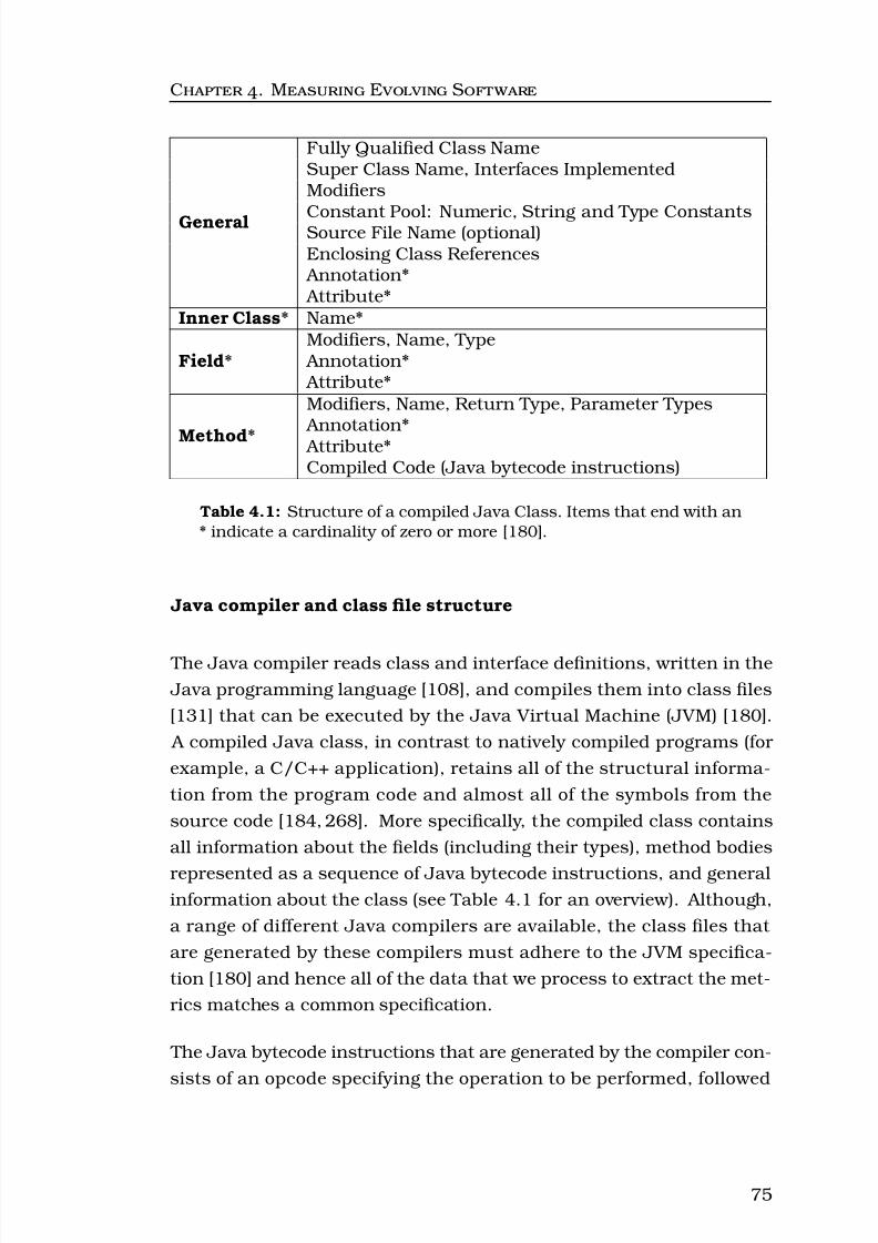
8/8/2019 Rajesh Vasa -- PhD Thesis
http://slidepdf.com/reader/full/rajesh-vasa-phd-thesis 94/252
C . M E S
General
Fully Qualified Class NameSuper Class Name, Interfaces ImplementedModifiers
Constant Pool: Numeric, String and Type ConstantsSource File Name (optional)Enclosing Class References
Annotation* Attribute*
Inner Class* Name*
Field*Modifiers, Name, Type
Annotation* Attribute*
Method*
Modifiers, Name, Return Type, Parameter Types Annotation* Attribute*Compiled Code (Java bytecode instructions)
Table 4.1: Structure of a compiled Java Class. Items that end with an* indicate a cardinality of zero or more [180].
Java compiler and class file structure
The Java compiler reads class and interface definitions, written in the
Java programming language [108], and compiles them into class files
[131] that can be executed by the Java Virtual Machine (JVM) [180].
A compiled Java class, in contrast to natively compiled programs (for
example, a C/C++ application), retains all of the structural informa-
tion from the program code and almost all of the symbols from the
source code [184, 268]. More specifically, the compiled class contains
all information about the fields (including their types), method bodies
represented as a sequence of Java bytecode instructions, and generalinformation about the class (see Table 4.1 for an overview). Although,
a range of different Java compilers are available, the class files that
are generated by these compilers must adhere to the JVM specifica-
tion [180] and hence all of the data that we process to extract the met-
rics matches a common specification.
The Java bytecode instructions that are generated by the compiler con-
sists of an opcode specifying the operation to be performed, followed
75

8/8/2019 Rajesh Vasa -- PhD Thesis
http://slidepdf.com/reader/full/rajesh-vasa-phd-thesis 95/252
C . M E S
1 /∗∗ A simple method to print "Hello World" to console ∗/
2 public void printHelloWorld ( )
3 {
45 System . out . println ( " Hello World" ) ;
6
7 // Annotated bytecode instructi ons
8 // Numbers that start with a # are the index into the constant pool
9
10 // getstat ic #5; //LOAD Field java/lang/System.out: java/io/PrintStream
11 // ldc #6; //LOAD String Hello World
12 // invoke virtual #7; //CALL Method j ava/io/PrintStream. printl n
13 // return
14 }
Listing 4.1: Same of bytecode generated for a simple Hello World
method
by zero or more operands which contain the values to be operated
upon [180]. There are a total of 256 possible opcodes instructions that
can be generated by the compiler and all of these instructions are em-
bedded in the method body (see Table 4.1). We process the bytecode
instructions and determine the nature of the operation in order to com-pute appropriate metrics. The sample code in Listing 4.1 for a “Hello
World” method shows the set of bytecode instructions that are gener-
ated as comments within the method body. In this sample listing, there
are 4 bytecode instructions generated from a single line of source code
(three bytecode instructions take a single operand, while one of the op-
erations has zero operands). In our study, we process these bytecode
instructions, as well as all of the other information embedded in the
compiled class (as indicated in Table 4.1) to compute the various met-
rics. A fully annotated Java program is presented in Appendix D to
further illustrate how our metric extraction approach counts the vari-
ous metrics from the compiled class file.
Differences between source code and compiled code
Though, the compiled Java class is close to the source code, there are
some differences:
76

8/8/2019 Rajesh Vasa -- PhD Thesis
http://slidepdf.com/reader/full/rajesh-vasa-phd-thesis 96/252

8/8/2019 Rajesh Vasa -- PhD Thesis
http://slidepdf.com/reader/full/rajesh-vasa-phd-thesis 97/252
C . M E S
sub-set of classes that they use from this package. Furthermore,
the type names within the source code typically contain just the
class name, not the fully qualified name (for example, it is more
common to use Math rather than java.lang.Math when the de-
velopers rely on mathematical library functions).
• All comments are removed from compiled class files.
• The compilation process typically erases local variable names and
hence we lose these symbol names in the compiled class.
• A compiled class contains a constant pool which is an array con-
taining all the numeric, string and type constants that are used in
the class. These constants are defined only once in the constant
pool and referenced (via an index) in all other sections of the class.
Metrics Extraction and Post Processing
We process each compiled Java class file and extract two types of met-
rics: direct count metrics and modifier flags. Table 4.2 shows the list of
count metrics that we extract by processing field and method interfaceinformation for each class, Table 4.3 shows the list of count metrics
that are computed by processing the bytecode instructions present in
method bodies, and Table 4.4 shows the flags that we extract for each
class. In this thesis, we treat all the count metrics as measures of size
as they reflect size of a class from different perspectives. However, we
consider the Number of Branches (NOB) measure as a complexity met-
ric that captures the internal structure of a class. The NOB measure is
equivalent to the widely used Weighted Method Count (WMC) metric [46]
with Cyclomatic Complexity [190] used as the weight [46]. The WMC
and (hence our formulation of the NOB) is accepted within the literature
as a measure of structural complexity [116, 165].
Along with the metrics shown in Tables 4.2, 4.3, and 4.4 we also capture
the fully qualified name of each class, its fully-qualified super class
name as well as all method names (including full signature capturing
the return type), field names (including the type) and the fully-qualified
name of all other classes that a class depends upon.
78

8/8/2019 Rajesh Vasa -- PhD Thesis
http://slidepdf.com/reader/full/rajesh-vasa-phd-thesis 98/252
C . M E S
Abbv. Name Description
NOM Method Count Number of methods AMC Abstract
Method Count Number of abstract methods
RMC ProtectedMethod Count
Number of protected methods
PMC Public MethodCount
Number of public methods
IMC Private MethodCount
Number of private methods
SMC Static Method
Count
Number of methods with a static modifier
FMC Final MethodCount
Number of methods with a final modifier
YMC SynchronizedMethod Count
Number of methods with a synchronizedmodifier
NOF Field Count Number of fields definedPFC Public Field
Count Number of fields with a public modifier
IFC Private FieldCount
Number of fields with a private modifier
RFC Protected FieldCount Number of fields with a protected modifier
FFC Final FieldCount
Number of fields with a final modifier
SFC Static FieldCount
Number of fields defined with a static modi-fier
ZFC Initialized FieldCount
Number of fields initialised when declared
UFC UninitializedField Count
Number of fields uninitialized when declared
INC Interface Count Number of interfaces implemented.EXC Exception
Count Number of exceptions raised by the methods
CCC Class Construc-tor Count
Number of constructors defined. This value will always be ≥ 1 since the compiler alwaysgenerates a default constructor, even if one
was not provided in the source code.
Table 4.2: Direct count metrics computed for both classes and inter-faces.
79

8/8/2019 Rajesh Vasa -- PhD Thesis
http://slidepdf.com/reader/full/rajesh-vasa-phd-thesis 99/252

8/8/2019 Rajesh Vasa -- PhD Thesis
http://slidepdf.com/reader/full/rajesh-vasa-phd-thesis 100/252
C . M E S
Abbv. Name DescriptionIAS Is Abstract A flag that is set to 1, if class is abstract IEX Is Exception A flag that is set to 1 if class has
java.lang.Throwable as an ancestor INF Is Interface A flag that is set to 1 if class is an interfaceIPI Is Private A flag that is set to 1 if class is privateIPR Is Protected A flag that is set to 1 if class is protectedIPU Is Public A flag that is set to 1 if class is publicIPK Is Package
Accessible A flag that is set to 1 if the class has no visibility modifier and hence would revert tohaving package visibility
Table 4.4: Flags extracted for each class.
Once information from all the classes is extracted, we remove classes
that are from external libraries that are not part of the core software
system under study. Though, we ensure that the set of input JAR files
used in the Jar Extraction step does not consist of any external libraries
(see Section 4.5.1), this additional step was needed since some projects
merged all external library code into their core JAR file in order to re-
duce the number of different files that needed to be distributed. We
identify and removed the set of classes that are from external librariesusing the same process that we applied during the Jar Extraction step
(see Section 4.5.1).
The Java programming language provides developers the option for cre-
ating two different types of abstractions: a class, and an interface [108].
Within the context of our study, the key distinction between these two
abstractions is that interfaces do not contain any method bodies and
hence the metrics defined in Table 4.3 are not available for compiled
Java interfaces which do not contain bytecode instructions in the method
section of a class file. However, all of the other information (see Ta-
ble 4.1) is available and therefore used to compute the metrics defined
in Table 4.2 and Table 4.4. We are also able to extract dependency infor-
mation from an interface, that is, other Java classes that an interface
depends upon (discussed in Section 4.5.4). In the rest of this thesis, to
improve readability, we use the term class to indicate a compiled Java
class, and it may be either a Java interface or a Java class. We use
81

8/8/2019 Rajesh Vasa -- PhD Thesis
http://slidepdf.com/reader/full/rajesh-vasa-phd-thesis 101/252
C . M E S
the terms Java Interface and Java Class where these abstractions are
treated separately in our analysis.
4.5.3 Merge Inner Classes
In Java, the inner class abstraction is provided as a convenience mech-
anism to structure the functionality within a class [125]. For example,
inner classes are commonly used to implement event handlers in graph-
ical user interface applications. More generally, inner classes are used
when an object needs to send another object a block of code that can
call the first object’s methods or manipulate its instance variables.
Interestingly, the Java virtual machine specification [180] requires the
compiler to emit a separate class file for each class including the inner
classes defined within a class (of Java source code). However, semanti-
cally developers consider inner-classes to be a part of the parent class
within the solution design. Especially since instances of an inner class
cannot be instantiated without being bound to an enclosing class.
In the Metric Extraction step, inner classes are processed as separateentities since we use compiled class files as input. However, for the
purposes of our study, we treat inner classes as part of the parent class
and hence merge all metrics collected from inner classes into the parent
class. The key benefit gained by merging is that is allows us to focus
on the core abstractions within the solution rather than the specific
internal representation of a class. However, the trade-off is that we
are unable to directly observe the evolution dynamics of inner classes
independent of their parent classes.
4.5.4 Class Dependency Graph Construction
In order to measure the structural complexity of a software system we
construct a complete class dependency graph, GT and measure certain
properties of this graph. When a class uses either data or functionality
from another class, there is a dependency between these classes. In
the context of Java software, a dependency is created if a class inher-
82

8/8/2019 Rajesh Vasa -- PhD Thesis
http://slidepdf.com/reader/full/rajesh-vasa-phd-thesis 102/252
C . M E S
Classes in set K
Classes in set N
Java Framework
Math Date
Third-Party Library
BC
A
Core Software System
QR
S T
U V
Figure 4.6: The dependency graph that is constructed includesclasses from the core, external libraries and the Java framework. Thetwo sets, N and K, used in our dependency graph processing are high-lighted in the figure.
its from a class, implements an interface, invokes a method on another class (including constructors), declares a field or local variable, uses an
exception, or uses class types within a method declaration. The depen-
dency graph contain nodes representing the classes in the system, and
directed links which represent the dependencies between these classes.
During the construction of Java software systems it is common for de-
velopers to make use of third-party libraries, as well as functionality
provided in the Java framework (which is distributed as part of the
Java Runtime Environment). Therefore, a dependency can be created
between classes inside the core software system as well as to classes
external to the software system. The dependency graph GT that we
construct contains nodes represented by classes from the core software
system, external libraries as well as the Java framework.
We capture the relationship between two classes as a directed link (edge)
in the dependency graph GT as this allows us to determine the set of
incoming links (the in-degree ) into a class as well as the set of outgoing
83

8/8/2019 Rajesh Vasa -- PhD Thesis
http://slidepdf.com/reader/full/rajesh-vasa-phd-thesis 103/252
C . M E S
links from a class (the out-degree ). As discussed in Section 4.2.2, these
two measures are widely used in the literature as measures of struc-
tural complexity [21, 54, 55, 77, 117, 165, 209, 223, 287, 294, 299] since
they naturally capture the number of classes a given class X depends
upon and the number of classes that depend on X.
For the purpose of measuring the dependencies we define two sets K
and N . The first set, K is a finite non-empty set of all classes in the
software system and includes the classes from the core software system,
as well as classes that provide services (to classes in the core) but are in
part of third-party libraries or the Java framework. The second set, N
contains classes that are part of the core software system such that N ⊂K. The distinction between these two sets is illustrated in Figure 4.6.
The type dependency graph GT is an ordered pair < K, L >, where L
is a finite, possibly empty, set of directed links between classes, such
that, L ⊆ N × K. Our restriction of focusing on the core software sys-
tem (as discussed in Section 3.6.2) implies that we do not measure the
dependencies between classes in the external libraries and hence we
analyze only the set of links that are formed when classes within the
set N depend on classes in the set K. For example, the dependency
between classes A and B in Figure 4.6 is not part of the graph that we
construct. Additionally, classes A and B in Figure 4.6 are also not in
the set K.
4.5.5 Dependency Metric Extraction
Once the dependency graph has been constructed, we can analyze eachnode n ∈ N in the graph as well as the set of directed links l ∈ L for
each node within the graph GT and measure the In-Degree Count lin(n),
as well as the Out-Degree Count lout (n) it. More precisely,
lin(n) = |{(ni, n) ∧ ni ∈ N ∧ n = ni}| (4.5.1)
84

8/8/2019 Rajesh Vasa -- PhD Thesis
http://slidepdf.com/reader/full/rajesh-vasa-phd-thesis 104/252
C . M E S
Abbv. Name Description
ODC Out Degree Count Number of classes that this class de-pends upon. Metric is defined by
lout (n) and the values are within theinterval [0, |K|).IDC In Degree Count Number of classes that depend on
this class. Metric is defined by lin(n)and the values are within the interval[0, |N |).
EDC External Out DegreeCount
Number of classes that this classclasses depends upon, but belong inexternal libraries. Metric is defined
by leout (n) and the values are within
the interval [0, |K|). TDC Internal Out DegreeCount
Number of classes that depend onthis class and are part of the coresoftware system. Metric is defined by liout (n) and the values are within the
interval [0, |N |).
Table 4.5: Dependency metrics computed for each class.
lout (n) = |{(n, n j) ∧ n j ∈ K ∧ n = n j}| (4.5.2)
The In-Degree Count is a measure of the “popularity" of node n in the
graph GT whereas the Out-Degree Count is node n’s “usage" of other
types in the graph GT [223].
We further refine the notions of in-degree and out-degree in the con-
text of our analysis by considering dependencies to classes in external
libraries. These external dependencies give rise to a refinement of the
measures in-degree and out-degree in which we also distinguish be-
tween intra- and inter- system links. A given link to or from a node n
may or may not cross the boundary of the containing core system, de-
pending on some organizational, structural, and/or functional features.
If an outbound link from node n ends in a node nint that occurs within
the boundary of the system under analysis, then we call this link an
internal outbound link. On the other hand, if an outbound link ends
in a node next that lies outside of the system’s boundary, then we call
85

8/8/2019 Rajesh Vasa -- PhD Thesis
http://slidepdf.com/reader/full/rajesh-vasa-phd-thesis 105/252
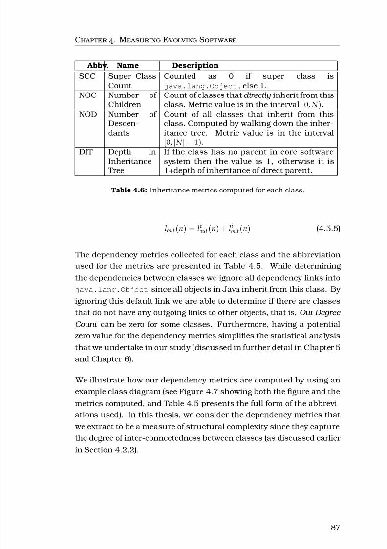
8/8/2019 Rajesh Vasa -- PhD Thesis
http://slidepdf.com/reader/full/rajesh-vasa-phd-thesis 106/252
C . M E S
Abbv. Name Description
SCC Super ClassCount
Counted as 0 if super class isjava.lang.Object, else 1.
NOC Number of Children
Count of classes that directly inherit from thisclass. Metric value is in the interval [0, N ).
NOD Number of Descen-dants
Count of all classes that inherit from thisclass. Computed by walking down the inher-itance tree. Metric value is in the interval[0, |N | − 1).
DIT Depth inInheritance
Tree
If the class has no parent in core softwaresystem then the value is 1, otherwise it is1+depth of inheritance of direct parent.
Table 4.6: Inheritance metrics computed for each class.
lout (n) = leout (n) + li
out (n) (4.5.5)
The dependency metrics collected for each class and the abbreviation
used for the metrics are presented in Table 4.5. While determining
the dependencies between classes we ignore all dependency links into
java.lang.Object since all objects in Java inherit from this class. By ignoring this default link we are able to determine if there are classes
that do not have any outgoing links to other objects, that is, Out-Degree
Count can be zero for some classes. Furthermore, having a potential
zero value for the dependency metrics simplifies the statistical analysis
that we undertake in our study (discussed in further detail in Chapter 5
and Chapter 6).
We illustrate how our dependency metrics are computed by using an
example class diagram (see Figure 4.7 showing both the figure and the
metrics computed, and Table 4.5 presents the full form of the abbrevi-
ations used). In this thesis, we consider the dependency metrics that
we extract to be a measure of structural complexity since they capture
the degree of inter-connectedness between classes (as discussed earlier
in Section 4.2.2).
87

8/8/2019 Rajesh Vasa -- PhD Thesis
http://slidepdf.com/reader/full/rajesh-vasa-phd-thesis 107/252
C . M E S
ClassA
ClassC
java.lang.Object
ClassB ClassD
ClassE
Class SCC NOC NOD DIT
ClassA 0 3 4 1ClassB 1 0 0 2ClassC 1 0 0 2ClassD 1 1 1 2ClassE 1 0 0 3
Figure 4.8: Class diagram to illustrate how inheritance metrics arecomputed. The metrics for the diagram shown in the table below thediagram.
4.5.6 Inheritance Metric Extraction
The final step in our metric extraction process focuses on measuring in-
heritance. The set of inheritance measures that we compute are listed
and explained in Table 4.6. We illustrate how our inheritance met-
rics are computed by using an example class diagram (see Figure 4.8
showing both the figure and the metrics computed). Since we do not
process classes external to the core software system, the inheritance
measures that we compute may not include the complete set of ances-
tors for any given class in a software system. For example, consider a
class ReportView that extends the class javax.swing.JFrame which
is part of the Java framework. We compute the inheritance metric Depth
88

8/8/2019 Rajesh Vasa -- PhD Thesis
http://slidepdf.com/reader/full/rajesh-vasa-phd-thesis 108/252
C . M E S
of Inheritance Tree to have a value of 1. However, if the Java framework
was fully analysed then this would change to 6 (for Java 1.6), since we
now are processing the full extent of the inheritance chain by extracting
additional information from the external Java framework. Though our
metrics are constrained, the inheritance hierarchy within the external
framework was designed and created by an external team and hence all
changes to it are outside of the direct control of the development team
creating the software under study. Hence, we do not measure the inher-
itance hierarchies of external libraries and the core Java framework as
part of our analysis. Furthermore, we do not consider interface imple-
mentation as inheritance and hence do not count them in our metrics.
4.6 Summary
The evolution of a software system can be studied in terms of how var-
ious properties as reflected by software metrics change over time. We
build a release history model by analysing the compiled class files. Our
release history model captures meta-data and 58 different metrics at a
class level. We also build a class dependency graph for each release inthe evolution history.
The data selection and metric extraction method that we use ensures
that we study non-trivial software allowing us to extend our findings
to other comparable software systems built in Java. We also analyse
compiled binaries that have already gone through the build process
improving the accuracy of our measures. Further, as discussed in the
previous chapter, we focus on contributions from the core development team ignoring third party libraries ensuring that the metrics that we
collect are a better reflection of the development effort.
The next chapter (Growth Dynamics) addresses the research questions
related to growth. We describe how size and complexity is distributed
as systems evolve and present a novel analysis technique to help un-
derstand growth dynamics.
89
8/8/2019 Rajesh Vasa -- PhD Thesis
http://slidepdf.com/reader/full/rajesh-vasa-phd-thesis 109/252
Chapter 5
Growth Dynamics
Current models of software evolution [118,119,127,153,168,175,200,
217, 239, 277, 284, 305, 310] have allowed for inferences to be drawn
about certain attributes of the software system, for instance, regarding
the architecture [100, 101, 127, 153, 192, 200], complexity and its im-
pact on the development effort [118, 168, 284]. However, an inherent
limitation of these models is that they do not provide any direct insight
into where growth takes place. In particular, we cannot assess the
impact of evolution on the underlying distribution of size and complex-
ity among the various classes. Such an analysis is needed in order to
answer questions such as “do developers tend to evenly distribute com-
plexity as systems get bigger?” and “do large and complex classes get
bigger over time?” . These are questions of more than passing interest
since by understanding what typical and successful software evolution
looks like, we can identify anomalous situations and take action earlier
than might otherwise be possible. Information gained from an analy-sis of the distribution of growth will also show if there are consistent
boundaries within which a software design structure exists.
The specific research questions that we address in this chapter are:
• What is the nature of distribution of software size and complexity
measures?
90

8/8/2019 Rajesh Vasa -- PhD Thesis
http://slidepdf.com/reader/full/rajesh-vasa-phd-thesis 110/252
C . G D
• How does the profile and shape of this distribution change as soft-
ware systems evolve?
• Is the rate and nature of change erratic?
• Do large and complex classes become bigger and more complex as
software systems evolve?
The typical method to answer these questions is to compute traditional
descriptive statistical measures such as arithmetic mean (referred to as
“mean” in the this thesis to improve readability), median and standard
deviation on a set of size and complexity measures and then analyze
their changes over time. However, it has been shown that software size
and complexity metric distributions are non-gaussian and are highly
skewed with long tails [21, 55, 270]. This asymmetric nature limits
the effectiveness of traditional descriptive statistical measures such as
mean and standard deviation as these values will be heavily influenced
by the samples in the tail making it hard to derive meaningful infer-
ences.
Recently advocated alternative method to analyze metric distributions[21,55,118,223, 270, 299] involves fitting metric data to a known prob-
ability distribution. For instance, statistical techniques can be used to
determine if the metric data fits a log-normal distribution [55]. Once a
strong fit is found, we can gain some insight into the software system
from the distribution parameters. Unfortunately, the approach of fit-
ting data to a known distribution is more complex and the metric data
may not fit any known and well understood probability distributions
without a transformation of the data.
Software metrics, it turns out, are distributed like wealth in society —
where a few individuals have a high concentration of wealth, while the
majority are dispersed across a broad range from very poor to what
are considered middle class. To take advantage of this nature, we ana-
lyze software metrics using the Gini coefficient , a bounded higher-order
statistic [191] widely used in the field of socio-economics to study the
distribution of wealth and how it changes over time. Specifically it is
91

8/8/2019 Rajesh Vasa -- PhD Thesis
http://slidepdf.com/reader/full/rajesh-vasa-phd-thesis 111/252
C . G D
used to answer questions like “are the rich getting richer?”. Our ap-
proach allows us not only to observe changes in software systems ef-
ficiently, but also to assess project risks and monitor the development
process itself. We apply the Gini coefficient to 10 different metrics and
show that many metrics not only display consistently high Gini values,
but that these values are remarkably consistent as a project evolves
over time. Further, this measure is bounded (between a value of 0 and
1) and when observed over time it can directly inform us if develop-
ers tend to centralise functionality and complexity over time or if they
disperse it.
The rest of this chapter is structured as follows: Section 5.1 presentsan overview of the nature of the software metric data and summarises
the current approaches used to analyse this data and their limitations.
Section 5.2 presents the Gini Coefficient that we use to understand
software metric data and show how it overcomes the limitations of the
statistical techniques applied in work by other researchers. Section 5.3
presents the analysis approach and shows how we apply the Gini Co-
efficient to address the research questions. Section 5.4 summarises
the observations while Section 5.5 discusses our findings and offers aninterpretation.
The raw data used is this study is available as data files on the DVD
attached to this thesis. Appendix E describes the various data and
statistical analysis log files related to this chapter.
5.1 Nature of Software Metric Data
A general characteristic of object oriented size and complexity metrics
data is that they are heavily skewed with long-tails [21, 55, 118, 223,
270, 299]. It has been shown that small values are extremely common,
while very large values can occur, they are quite rare. Typically soft-
ware systems follow a simple pattern: a few abstraction contain much
of the complexity and functionality, whereas the large majority tend to
define simple data abstractions and utilities. This pattern is illustrated
in Figure 5.1 with one metric, the Number of Methods in a class for ver-
92

8/8/2019 Rajesh Vasa -- PhD Thesis
http://slidepdf.com/reader/full/rajesh-vasa-phd-thesis 112/252
C . G D
0
. 2
. 4
. 6
. 8
1
C u m u l a t i v e P e r c e n t a g e
0
5
1 0
1 5
P e r c e n t
0 20 40 60 80 100 120 140 160 180
Number of Methods
Figure 5.1: Relative and Cumulative frequency distribution showingpositively skewed metrics data for the Spring Framework 2.5.3. Theright y-axis shows the cumulative percentage, while the left side shows
the relative percentage.
sion 2.5.3 of the Spring Framework. As can be observed in the figure,
approximately 20% of the classes have more than 10 methods suggest-
ing that relatively few classes have a large number of methods in this
system. This skewed metric distribution pattern repeats for the differ-
ent metrics that we collect in our study across all the software systems
(discussed further in Section 5.4.2).
5.1.1 Summarising with Descriptive Statistics
The sheer volume of metric data available from any object-oriented soft-
ware systems can make it difficult to understand the nature of soft-
ware systems and how they have evolved [75]. A common approach
[77, 117, 165, 182] to reducing the complexity of the analysis is to ap-
ply some form of some simple statistical summarisation such as the
93

8/8/2019 Rajesh Vasa -- PhD Thesis
http://slidepdf.com/reader/full/rajesh-vasa-phd-thesis 113/252
C . G D
mean , median , or standard deviation . Unfortunately, these descrip-
tive statistics provide little useful information about the distribution
of the data, particularly if it is skewed, as is common with many soft-
ware metrics [21,55,118,223,270,299]. Furthermore, the typical long-
tailed metric distributions makes precise interpretation with standard
descriptive statistical measures difficult.
Commonly used summary measures such as “arithmetic mean” and
“variance” capture the central tendency in a given data set. However,
where the distribution is strongly skewed, they become much less re-
liable in helping understand the shape and changes in the underlying
distribution. Moreover, additional problems may arise due to changesin both the degree of concentration of individual values and the popu-
lation size. Specifically, since these summary measures are influenced
by the population size which tends to increase in evolving software sys-
tems.
Descriptive statistics such as median and variance are also likely to be
misleading, given the nature of the underlying distribution. Specifically,
we found that the median measure does not change substantially over
time reducing its effectiveness when applied to understanding software
evolution. An example of this is illustrated in Figure 5.2, where the
median of three different metrics is shown for PMD. As can be seen
in the figure, the median value is very stable over a period of nearly
5 years of evolution. Though there is some change (to the median), in
absolute terms the value does not convey sufficient information about
the nature and dynamics of the evolution.
Additional statistics such as the skew , which measures the asymme-try of the data, and kurtosis , which measures the peakedness of the
data, may be applied, but are ineffective for comparison between sys-
tems with different population sizes as these measures are unbounded
and change depending on the size of the underlying population, mak-
ing relative comparisons ineffective [221]. Given this situation, it is not
surprising that metrics use in industry is not widespread [137]. This
situation is also not helped by the current generation of software met-
ric tools as many commercial and open source tools [47,51, 196, 203,
94

8/8/2019 Rajesh Vasa -- PhD Thesis
http://slidepdf.com/reader/full/rajesh-vasa-phd-thesis 114/252
C . G D
0
1
2
3
4
5
6
M e d i a n
0 10 20 30 40
Release Sequence Number
Number of Methods Public Method Count
Out-Degree Count
Figure 5.2: Change in Median value for 3 metrics in PMD.
224, 226, 251, 274, 295, 296] summarise data using simple descriptivestatistical measures.
Comparison of different distributions may provide some insight, but re-
quire skill to interpret, particularly given the range of measures that can
be used and the different population sizes that might be encountered.
5.1.2 Distribution Fitting to Understand Metric Data
A more recent method to understand software metric data distribu-
tion involves fitting the data to a known probability distribution [21,55,
118, 223, 270, 299]. For example, statistical techniques can be used to
determine if the Number of Methods in a system fits a log-normal distri-
bution [55]. The motivation for fitting metrics to known distributions is
driven by the notion that it can help explain the underlying processes
that might be causing specific distributions [209,287]. Furthermore, if
the fit is robust and consistent we can infer information from the distri-
95

8/8/2019 Rajesh Vasa -- PhD Thesis
http://slidepdf.com/reader/full/rajesh-vasa-phd-thesis 115/252

8/8/2019 Rajesh Vasa -- PhD Thesis
http://slidepdf.com/reader/full/rajesh-vasa-phd-thesis 116/252

8/8/2019 Rajesh Vasa -- PhD Thesis
http://slidepdf.com/reader/full/rajesh-vasa-phd-thesis 117/252
C . G D
Though, fitting distributions has been shown to have merit for model-
ing networks [210] and to infer how these networks have been created,
software evolution is better modelled by analysing the evolution history
as we can reduce the number of assumptions one has to make. Rather
than attempting to infer the generative process from a single release of
a software system, we can gain more insight into the evolutionary pres-
sures by analysing the changing metric distribution over time. In our
work, we take this approach and study the metric distributions as they
change over time in order gain a better understanding of the underlying
evolutionary processes.
Though there has been progress over the last decade in this field, thereis still no widely-accepted distribution that captures consistently and
reliably software metric data. But more importantly, we are not re-
quired to fit a given software metric to particular distributions in order
to interpret it. What is needed is a set of measures that reliably and con-
sistently summarize properties of the distribution allowing for effective
inferences to be made about the evolution of a software system.
5.2 Summarizing Software Metrics
Given the skewed nature of metric data we are in need of methods that
can effectively summarise this data and provide effective insight into
the current state of a software system as well as detect worthwhile
changes as the software evolves. In this section we introduce the Gini
Coefficient, a measure that is effective when dealing with metric data
and motivate its applicability for analysing evolving metric data distri-
butions.
5.2.1 Gini Coefficient - An Overview
One of the key pieces of information we wish to obtain from software
metrics is the allocation of functionality within the system. Under-
standing whether the system has a few classes that implement most
of the methods or whether methods are widely distributed gives us an
98

8/8/2019 Rajesh Vasa -- PhD Thesis
http://slidepdf.com/reader/full/rajesh-vasa-phd-thesis 118/252
C . G D
insight into how the system has been constructed, and how to maintain
it [66]. A technique to study allocation of some attribute within a popu-
lation and how it changes over time has been studied comprehensively
by economists who are interested in the distribution of wealth and how
this changes [311] – we use the same approach in our analysis.
In 1912, the Italian statistician Corrado Gini proposed the Gini coef-
ficient , a single numeric value between 0 and 1, to measure the in-
equality in the distribution of income or wealth in a given population
(cp. [91, 229]). A low Gini coefficient indicates a relatively equal wealth
distribution in a given population, with 0 denoting a perfectly equal
wealth distribution (i.e., everybody has the same wealth). A high Ginicoefficient, on the other hand, signifies a very uneven distribution of
wealth, with a value of 1 signalling perfect inequality in which one in-
dividual possesses all of the wealth in a given population. The Gini
Coefficient is a widely used social and economic indicator to ascertain
an individual’s ability to meet financial obligations or to correlate and
compare per-capita GDPs [286].
We can adopt this technique and consider software metrics data as in-
come or wealth distributions . Each metric that we collect for a given
property, say the number of methods defined by all classes in an object-
oriented system, is summarized as a Gini coefficient, whose value in-
forms us about the degree of concentration of functionality within a
given system.
5.2.2 Computing the Gini Coefficient
Key to the analysis of the distribution of data and computation of the
Gini Coefficient is the Lorenz curve [183], an example of which is shown
in Figure 5.3.
A Lorenz curve plots on the y-axis the proportion of the distribution
assumed by the bottom x% of the population. The Lorenz curve gives a
measure of inequality within the population. A diagonal line represents
perfect equality. A line that is zero for all values of x < 1 and 1 for x = 1
99

8/8/2019 Rajesh Vasa -- PhD Thesis
http://slidepdf.com/reader/full/rajesh-vasa-phd-thesis 119/252
C . G D
Figure 5.3: Lorenz curve for Out-Degree Count in Spring framework inrelease 2.5.3.
is a curve of perfect inequality.
For a probability density function f (x) and cumulative density function
F(x), the Lorenz curve L(F(x)) is defined as:
L(F(x)) =
x−∞ t f (t) dt ∞−∞ t f (t) dt
(5.2.1)
The Lorenz curve can be used to measure the distribution of functional-
ity within a system. Figure 5.3 is a Lorenz curve for the Fan-Out Count
metric in the Spring framework release 2.5.3. Although the Lorenz
curve does capture the nature of distribution, it can be summarizedmore effectively by means of the Gini coefficient. The Gini coefficient is
defined as a ratio of the areas on the Lorenz curve diagram. If the area
between the line of perfect equality and Lorenz curve is A, and the area
under the Lorenz curve is B, then the Gini coefficient is A/( A + B) [311].
More formally, if the Lorenz curve is L(Y), then the Gini Coefficient is
defined as:
100

8/8/2019 Rajesh Vasa -- PhD Thesis
http://slidepdf.com/reader/full/rajesh-vasa-phd-thesis 120/252
C . G D
GiniCoefficient = 1− 2 1
0
L(Y) dY (5.2.2)
For a population of metric data xi, i = 1 to n, that are indexed in an
increasing order such that xi ≤ xi+1, the Gini Coefficient G is computed
as:
G =1
n(n + 1− 2(
∑ ni=1(n + 1− i)xi
∑ ni=1 xi
)) (5.2.3)
The Gini Coefficient is a higher order statistic as it is derived from the
Lorenz curve, which itself is a summary measure computed over a cu-
mulative probability distribution function.
5.2.3 Properties of Gini Coefficient
The Gini coefficient has a number of useful properties in that it is
bounded between 0 and 1, makes no assumptions as to the distribu-tion of the statistic under investigation, and can be compared between
differently sized populations. These properties makes it an ideal statis-
tic for comparing the distribution of metrics between software systems
as well as multiple releases of an evolving software system. Moreover,
the Gini coefficient provides a simple and intuitive means for qualitative
analysis of observed software properties.
The Gini Coefficient summarises data independent of its distribution.For example, if the data has a gaussian distribution then the Gini Co-
efficient value will be around 0.10 (exact value will depend on the shape
of the distribution). This is the case, since nearly half of the data have
a very similar range of values and hence, there is minimal inequality
in the data. However, when we compute the Gini Coefficient value for
a highly skewed log-normal distribution where there is substantial in-
equality in the data, the value will be typically well over 0.5.
101

8/8/2019 Rajesh Vasa -- PhD Thesis
http://slidepdf.com/reader/full/rajesh-vasa-phd-thesis 121/252
C . G D
5.2.4 Application of the Gini Coefficient - An Example
We illustrate the applicability and simplicity of using the Gini Coef-
ficient coefficient to measure the inequality within a software metric
distribution with an example. We first present the Gini Coefficient of
In-Degree Count for the Spring Framework and then contrast it with
the standard descriptive statistical measure of arithmetic mean, me-
dian, standard deviation and skewness for In-Degree Count .
In the first version of the Spring Framework, the Gini Coefficient value
for In-Degree Count is 0.62. Values of Gini Coefficient substantially
greater than 0 are indicative of a skewed distribution, where a small set of classes are very popular (since In-Degree Count is the wealth in our
case). Furthermore, in Spring Framework, the Gini Coefficient value
gradually increases over time from 0.62 to 0.71 over a period of 4 years
of evolution. The trend shows that over time, a small set of classes are
gaining popularity. This type of trend analysis is used by economists to
answer the question “are the rich getting richer?”.
In contrast to the Gini Coefficient, in the Spring Framework, the me-
dian value of In-Degree Count has remained unchanged at 1 for its entire
evolution history, while the mean has increased slightly from 2.3 to 3.3.
Neither of which provide us with sufficient information about the skew
in the distribution and the fact that the a few classes have slowly gained
in popularity. The standard deviation measure has also increased grad-
ually from 3.74 to 11.5. The standard deviation measure provides some
indication that the underlying data might have a few strong outliers,
however it does not inform us of the shape of the distribution. The
statistical measure of skewness can be used to gain additional infor-mation that can indicate the shape of the distribution. The measure of
skewness for In-Degree Count increases from 4.32 to 18.10. The positive
values for skewness do reveal that we have a long tail to the right of the
distribution with some classes that have very high In-Degree Count . We
can also infer from the increasing skewness that we have a potential in-
crease in the upper bound, that is the highest In-Degree Count value
is increasing. However, as discussed earlier, the measure of skewness
is influenced by the population size making the interpretation difficult
102

8/8/2019 Rajesh Vasa -- PhD Thesis
http://slidepdf.com/reader/full/rajesh-vasa-phd-thesis 122/252
C . G D
Name Rationale Description
Load Instruction Count (LIC) Responsibility Number of read instructions
Store Instruction Count (SIC) Responsibility Number of write instructions
Number of Branches (NOB) Complexity Degree of algorithmic branching
In-Degree Count (IDC) Popularity Number of classes depending on thisclass
Out-Degree Count (ODC) Delegation Number of classes used
Number of Methods (NOM) Decomposition Breadth of functional decomposition
Public Method Count (PMC) Interface Size Exposure of responsibility
Number of Attributes (NOA) InformationStorage
Density of information stored in class
Fan-Out Count (FOC) Delegation Degree of dependence on others
Type Construction Count (TCC) Composition Number of object instantiations
Table 5.1: Collected measures for distribution and change analysisusing the Gini Coefficient
without further analysis. Although, the different descriptive statisti-
cal measures (arithmetic mean, standard deviation, skewness) can be
combined to gain a picture of the underlying distribution, the Gini Co-
efficient provides a simpler and more direct method to measure the
inequality in a distribution.
5.3 Analysis Approach
In this section we present our analysis method. We first introduce the
set of metrics that were analysed using the Gini coefficient, followed by
the various steps in our analysis. We describe the observations arising
from our analysis in Section 5.4 and present a discussion of our findings
in Section 5.5.
5.3.1 Metrics Analyzed
In our study of metric distributions, we focused on 10 different mea-
sures that span a range of size and complexity measures. The selected
measures and a brief description of these metrics is provided in Ta-
ble 5.1.
In order to assess assigned responsibilities we use the two metrics Load
Instruction Count and Store Instruction Count . Both metrics provide a
103

8/8/2019 Rajesh Vasa -- PhD Thesis
http://slidepdf.com/reader/full/rajesh-vasa-phd-thesis 123/252

8/8/2019 Rajesh Vasa -- PhD Thesis
http://slidepdf.com/reader/full/rajesh-vasa-phd-thesis 124/252
C . G D
plifying models constructed to understand software. Similar to Succi
et al. [265], we compute the Spearman’s rank correlation coefficient ρ
and applied the t-test to check if the reported coefficient is different from
zero at a significance level of 0.05 for all 10 measures in all systems.
The t-test checks that the reported relationship between the Gini Coef-
ficient and Age (days since birth) can be considered to be statistically
significant, while the correlation coefficient reports the strength of the
relationship between the Gini Coefficient and Age. The non-parametric
Spearman’s correlation coefficient was selected over Pearson’s correla-
tion coefficient since as it does not make any assumptions about the
distribution of the underlying data [279], specifically it does not assume
that the data has a gaussian distribution.
5.3.3 Checking Shape of Metric Data Distribution
A consistent finding by other researchers [21, 55, 223, 270, 299] study-
ing software metric distributions has been that this data is positively
skewed with long-tails. Can we confirm this finding in our own data?
Further, will this shape assumption hold if metric data was observed
over time? We undertook this step in order to provide additional strength
to the current expectation that metric data is highly skewed.
For a population with values xi, i = 1 to n with a mean of µ and a
standard deviation of σ ,
MovementSkewness =1
n
n
∑ i=1
(xi − µ)3
σ 3(5.3.1)
In our analysis, we tested the metric data for each release over the en-
tire evolution history to ensure that the data did not have a gaussian
distribution by using the Shapiro-Wilk goodness of fit tests for normal-
ity [279] at a significance level of 0.05. The expectation is that the test
will show that the metric data is not normally distributed. Addition-
ally, to confirm that the distribution can be considered skewed we com-
puted the descriptive measure of movement skewness (See Equation
105

8/8/2019 Rajesh Vasa -- PhD Thesis
http://slidepdf.com/reader/full/rajesh-vasa-phd-thesis 125/252
C . G D
5.3.1) [121]. The skewness measure was computed to determine if the
data was positively skewed. A skewness value close to zero is an indi-
cator of symmetry in the distribution, while values over 1.0 are used as
an indicator of a moderate level of skewness in the underlying metric
data, and values over 3.0 are observable in data with significant degree
of skew [121]. The value of skewness is not bounded within a range and
hence the degree of skewness can only be interpreted qualitatively.
5.3.4 Computing Gini Coefficient for Java Programs
We compute the Gini Coefficient for each of the selected metrics (see Table 5.1) using the formula in Equation 5.2.3. There were, however,
some minor adjustments made to the calculation after taking into con-
sideration certain Java language features. When we process code for
metric extraction, we treat both Java classes and Java interfaces as ab-
stractions from which we can collect metrics (see Chapter 4). However,
Interfaces in Java are unable to include load or store actions, branch-
ing, method invocations, or type constructions, respectively. As a re-
sult, interfaces were excluded from these counts, but were included in
the Out-Degree Count , In-Degree Count , Number of Methods , and Public
Method Count measures. While interfaces in Java may include constant
field declarations [108], it was decided to also exclude them from the
Number of Attributes measure in order to focus more directly on field
usage within individual classes.
5.3.5 Identifying the Range of Gini Coefficients
In our study, we use the Gini coefficient as a means to summarise
the metric data distribution. But, do different systems have a simi-
lar range of Gini Coefficient values for any given metric? Though, the
current state of the art has not been able to establish if a certain class
of probability distribution functions fit metric data, a narrow boundary
for the Gini Coefficient values across different systems in our data set
will confirm certain consistency among how developers organise soft-
ware solutions. For instance, if the Gini coefficient for Load Instruction
106

8/8/2019 Rajesh Vasa -- PhD Thesis
http://slidepdf.com/reader/full/rajesh-vasa-phd-thesis 126/252
C . G D
Count is in a very narrow boundary when measured across a range
of software systems, it will be an indication that there are certain un-
derlying distribution preferences that are not directly problem domain
dependent.
Similarly, if the Gini Coefficient values of any system (for a selected met-
ric) are within a very narrow boundary over the entire evolution history,
then it is an indicator of organisation stability at the system level. For
example, consider a software system which has increased in size by
300%, but the Gini Coefficient for Number of Branches is between 0.78
and 0.81 over an evolution of 4 years. This minimal fluctuation can be
seen as an indicator of stability in how developers organise structurally complex classes. However, if Gini Coefficient values change substan-
tially over the evolution period across different systems then it is an
indication that evolutionary pressures do play a role in how developers
organise the solutions.
We compute the range (difference between minimum and maximum)
as well as the Inter-Quartile range of Gini Coefficient values for each
metric and each system in order to identify any typical boundaries for
a specific metric across all systems.
5.3.6 Analysing the Trend of Gini Coefficients
We analyse the trends in Gini Coefficient values over time to answer one
of our research questions - do developers create more complex and large
classes over time? . If we consistently observe that the value of the Gini
Coefficients increase over time, this is a strong indicator that developersdo tend to centralise functionality into a few complex and large abstrac-
tions as software evolves. However, if the Gini Coefficients decrease over
time, this then suggests that there are pressures that compel develop-
ment teams to reorganise the responsibilities more evenly. However, a
third alternative is that developers have a certain set of habitual pref-
erence and that software evolution does not impact on the underlying
distribution significantly – that is, the Gini Coefficients do not change
substantially over time. If the Gini Coefficients consistently do not show
107
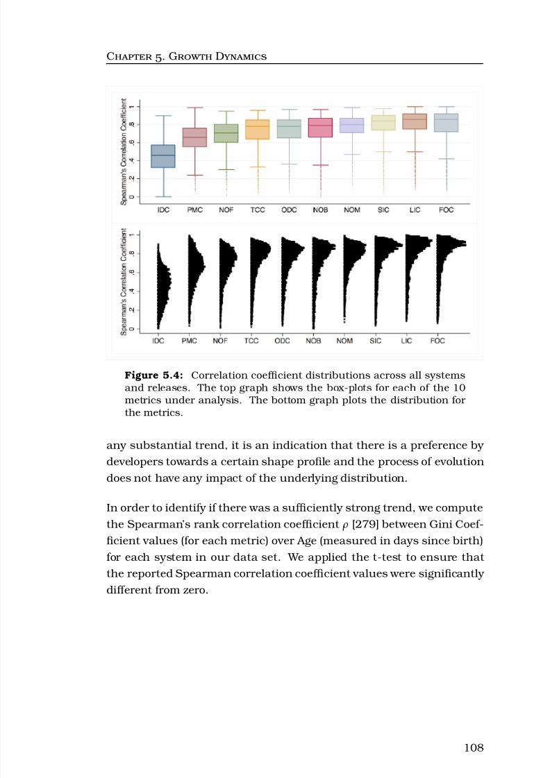
8/8/2019 Rajesh Vasa -- PhD Thesis
http://slidepdf.com/reader/full/rajesh-vasa-phd-thesis 127/252
C . G D
Figure 5.4: Correlation coefficient distributions across all systemsand releases. The top graph shows the box-plots for each of the 10metrics under analysis. The bottom graph plots the distribution for
the metrics.
any substantial trend, it is an indication that there is a preference by
developers towards a certain shape profile and the process of evolution
does not have any impact of the underlying distribution.
In order to identify if there was a sufficiently strong trend, we compute
the Spearman’s rank correlation coefficient ρ [279] between Gini Coef-
ficient values (for each metric) over Age (measured in days since birth)for each system in our data set. We applied the t-test to ensure that
the reported Spearman correlation coefficient values were significantly
different from zero.
108

8/8/2019 Rajesh Vasa -- PhD Thesis
http://slidepdf.com/reader/full/rajesh-vasa-phd-thesis 128/252
C . G D
LIC – SIC 0.93 – NOB 0.80 0.81 – IDC 0.18 0.24 0.15 –
ODC 0.86 0.82 0.77 0.08 – NOM 0.71 0.66 0.44 0.26 0.63 – PMC 0.21 0.20 0.09 0.27 0.18 0.75 – NOA 0.70 0.79 0.48 0.23 0.50 0.53 0.16 – FOC 0.96 0.87 0.80 0.09 0.85 0.62 0.16 0.67 – TCC 0.78 0.78 0.53 0.11 0.68 0.56 0.16 0.82 0.84 –
Metric LIC SIC NOB IDC ODC NOM PMC NOA FOC TCC
Table 5.2: Spearman’s Rank Correlation Coefficient values for one version (0.3.0) of JasperReports. Strong correlation values are high-lighted.
5.4 Observations
In this section we present our observations within the context of the
key research questions. The findings are summarised in Section 5.4.8
and discussed in Section 5.5.
5.4.1 Correlation between measures
As an initial step in our analysis to identify if a subset of the mea-
sures selected could be eliminated, we ran a correlation analysis be-
tween the 10 metrics under investigation (see Table 5.1). The range of
the observed correlation coefficient values is summarized (graphically)
in Figure 5.4 using both a box-plot as well as a histogram. The figure
shows, for each metric, the distribution of the correlation coefficient
against the other 9 metrics.
Our observations are summarised as follows:
• There exists a strong positive correlation (i.e., > 0.8 [265]) between
some different measures consistently across our entire data set.
The high correlation coefficient values can be seen in skewed his-
tograms chart in Figure 5.4 for most metrics. Across all system,
except for In-Degree Count and Public Method Count the correlation
coefficient values are in general very high.
109

8/8/2019 Rajesh Vasa -- PhD Thesis
http://slidepdf.com/reader/full/rajesh-vasa-phd-thesis 129/252
C . G D
• The strength of the relationship varies across systems and ver-
sions. For example, the measures Load Instruction Count and Fan-
Out Count are strongly correlated in JasperReports 0.3.0 (see Ta-
ble 5.2), but this relationship between Load Instruction Count and
Fan-Out Count is not as strong in other systems and releases.
• Across all systems, the measure In-Degree Count (IDC) consistently
shows the weakest correlation to other metrics suggesting that in
general, the popularity of a class is not a monotonic function of
the other metrics. This can be seen in Figure 5.4, where the IDC
metric value box plot as well as the distribution plot are signifi-
cantly different to that of all other metrics. Additionally, the out-liers shown in the box plot (outside the whiskers) are caused by
the IDC metric in all the other measures.
• Except for In-Degree Count , in 75% of the releases all other mea-
sures show moderate to high positive correlation (i.e. > 0.6) be-
tween different measures.
• Load Instruction Count and Store Instruction Count are in general
strongly correlated (i.e., over 0.8). This signifies that data often re-
quires a pair-wise read and write. However, there was one system,
rssOwl where the correlation was consistently weak. In rssOwl
the correlation coefficient value between Load Instruction Count
and Store Instruction Count is below 0.5 during the entire evolution
history, which is well below the typical expectation of a value well
over 0.8. The low correlation value observed in rssOwl was caused
by many classes loading a disproportionate amount of string con-
stants in the user interface classes as well as in classes providing
internationalization support. The typical strategy employed to loadlarge number of strings is to load the data from external resource
configuration files rather than by hard coding them in the source
code.
Our observations suggest that there is a consistent correlation between
the various internal size and internal structural complexity metrics of
a class. However, the popularity of a class (as measured by IDC) is not
a monotonic function of its size or internal complexity indicating that
110

8/8/2019 Rajesh Vasa -- PhD Thesis
http://slidepdf.com/reader/full/rajesh-vasa-phd-thesis 130/252
C . G D
large and complex classes need not directly service a large number of
other classes.
5.4.2 Metric Data Distributions are not Normal
Software systems that we analysed contained many hundreds of classes.
But how are they distributed? Are they highly skewed, as found by other
researchers? When we analysed this data, we found that our observa-
tions confirm findings from other researchers [21, 55, 223, 270, 299], in
that they do not fit a gaussian distributions. Further, we consistently
found positive values for skewness clearly indicating that in all casesthe distributions are skewed to contain a fat tail.
An example typical of the metric data in our data set is illustrated in Fig-
ure 5.1 and it shows the relative frequency distributions, for the metrics
Number of Methods and Fan-Out Count for release 2.5.3 of the Spring
framework (a popular Java/J2EE light-weight application container).
In both cases the distributions, are significantly skewed. However, the
shape of distribution is different. This is a pattern that is recurring
and common, that is, though the distributions are non-guassian and
positively skewed with fat tails, they are different for different systems
and metrics. A complete list of all descriptive statistics and the result
from our test for normality is presented in Appendix E.
5.4.3 Evolution of Metric Distributions
The upper and lower boundaries of the metric data distribution is bounded
within a fairly narrow range. Figure 5.5 presents the boundaries of the
histograms based on the minimum and maximum values of Number of
Branches , In-Degree Count , Number of Methods and Out-Degree Count
attained across all versions of the Spring Framework. The figures show
that relative frequency distributions of these measures have a distinct
profile that is bounded in a small range. The notable fact is that this
remarkable stability is observable over an evolution period of 5 years.
111

8/8/2019 Rajesh Vasa -- PhD Thesis
http://slidepdf.com/reader/full/rajesh-vasa-phd-thesis 131/252
C . G D
0.0%
5.0%
10.0%
15.0%
20.0%
25.0%
30.0%
35.0%
40.0%
45.0%
50.0%
0 1 2 3 4 5 6 7 8 9 10 11 12 13 14 15 16 17 18 19 20 21 22 23 24+
% C
l a s s e s
Number of Branches
0.0%
5.0%
10.0%
15.0%
20.0%
25.0%
30.0%
35.0%
40.0%
45.0%
0 1 2 3 4 5 6 7 8 9 10 11 12 13 14 15 16 17 18 19 20 21 22 23 24
% C
l a s s e s
In-Degree Count
0.0%
2.0%
4.0%
6.0%
8.0%
10.0%
12.0%
14.0%
16.0%
18.0%
20.0%
0 1 2 3 4 5 6 7 8 9 1 0 1 1 1 2 1 3 1 4 1 5 1 6 1 7 1 8 1 9 2 0 2 1 2 2 2 3 2 4 2 5 2 6 2 7 2 8 2 9
+
%
C l a s s e s
Method Count
0.0%
2.0%
4.0%
6.0%
8.0%
10.0%
12.0%
14.0%
16.0%
18.0%
20.0%
0 1 2 3 4 5 6 7 8 9 10 11 12 13 14 15 16 17 18 19 20 21 22 23 24 25 26 27 28 29+
%
C l a s s e s
Out-Degree Count
Figure 5.5: Spring evolution profiles showing the upper and lower boundaries on the relative frequency distributions for Number of Branches , In-Degree Count , Number of Methods and Out-Degree Count . All metric values during the entire evolution of 5 years fall within the
boundaries shown. The y-axis in all the charts shows the percentageof classes (similar to a histogram).
A similar phenomenon was observed across multiple projects for the
metrics under study. The profile of the relative frequency distribution
of all the metrics hold their broad shape across the evolutionary history
of any given software system. For example, if 20% of the classes in a
system have a In-Degree Count of 5 or greater in Version 1, the proba-
bility that this value will change by more than a few percent is very low
over the evolutionary history of the product. This holds for all of the various values of the other distributions as well.
There are however, some exceptions to this rule that coincide with struc-
tural shifts from one major release to another. For instance, in Hiber-
nate, one of the systems in our study, we noticed the profile of many
distributions has shifted significantly, twice during its evolutionary his-
tory. Upon closer examination we found that the profile shifted to a
new bounded range when the team moved from one major version to
112

8/8/2019 Rajesh Vasa -- PhD Thesis
http://slidepdf.com/reader/full/rajesh-vasa-phd-thesis 132/252
C . G D
0%
5%
10%
15%
20%
25%
30%
35%
0 1 2 3 4 5 6 7 8 9 10 11 12 13 14 15 16 17 18 19 20 21 22 23 24+
% C
l a s s e s
In-Degree CountHibernate 1.x Hibernate 2.x Hibernate 3.x
Figure 5.6: The distinct change in shape of the profile for Hibernateframework between the three major releases. Major releases were ap-proximately 2 years apart.
another with a different underlying structure. In the case of the Hiber-
nate framework, different distribution shapes can be seen in Figure 5.6
between three major releases. This observation also corresponds with
the release notes that indicate that the development team have under-taken substantial changes to the underlying structure and functionality
of the software system. Though, substantial changes are evident, this
is not the norm and in most cases the distributions can be considered
to be stable.
5.4.4 Bounded Nature of Gini Coefficients
Given the observed bounded range visually, do the Gini Coefficients
confirm a similar pattern? Do developers across domains tend to struc-
ture software similarly? Are there any bounds that they consistently
do not cross? In order to understand the underlying distribution from
a statistical perspective, we computed the Gini coefficients for the 10
metrics as outlined in Table 5.1.
The typical range for the Gini coefficient independent of the metric or
system under consideration is between 0.47 and 0.75, with a mean value
113

8/8/2019 Rajesh Vasa -- PhD Thesis
http://slidepdf.com/reader/full/rajesh-vasa-phd-thesis 133/252
C . G D
Metric Minimum Maximum Range
Load Instruction Count 0.60 0.64 0.04
Store Instruction Count 0.63 0.68 0.05
Number of Branches 0.68 0.72 0.04
In-Degree Count 0.62 0.72 0.10
Out-Degree Count 0.45 0.49 0.04
Number of Methods 0.48 0.56 0.08
Public Method Count 0.47 0.56 0.09
Number of Attributes 0.57 0.67 0.10
Fan-Out Count 0.62 0.66 0.04
Type Construction Count 0.66 0.80 0.14
Table 5.3: Gini value ranges in Spring Framework across 5 years of evolution
at approximately 0.65 (see Figure 5.7 for a box-plot). However, individualmetrics across all systems fell within a narrower boundary. The inter-
quartile-range (IQR) for Gini coefficients for any individual metric was
within a very small range of 0.15.
When any single system is considered, the range (difference of maxi-
mum and minimum) for all metrics falls within an even smaller range
across the entire evolutionary history. Table 5.3 shows the tight range
of Gini values for the Spring Framework over 5 years of evolution. In
22 systems the Gini range across all metrics under investigation was
under 0.10. In the remaining systems a couple of strong outliers pushed
the range out to approximately 0.20. The metric that has the greatest
range, is IDC, while the one that has the smallest range is ODC. Except
for IDC all other metrics (across all systems) have a typical range well
under 0.10.
Though, the relatively high value for Gini coefficient was not surprising
(given that metric distributions are known to be skewed), the narrow range for the IRQ confirms the visual observation that metric distribu-
tions do not change substantially over time.
Another observation we made is that it is rare to see Gini coefficients
greater than 0.8. For example, we noticed that in Struts, a Web applica-
tion framework, the Gini coefficient for In-Degree Count initially moves
beyond this threshold, only to fall back below it within a few releases
(see Figure 5.8). This interesting behaviour suggests that, in order for
114
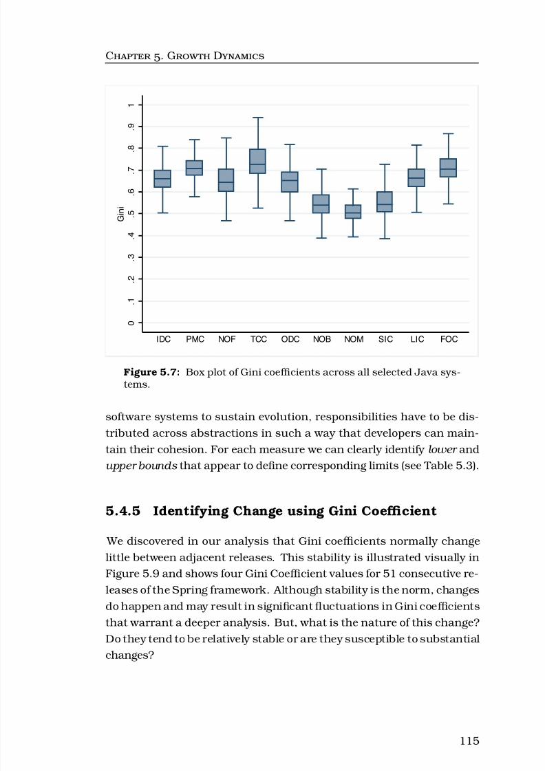
8/8/2019 Rajesh Vasa -- PhD Thesis
http://slidepdf.com/reader/full/rajesh-vasa-phd-thesis 134/252
C . G D
0
. 1
. 2
. 3
. 4
. 5
. 6
. 7
. 8
. 9
1
G i n i
IDC PMC NOF TCC ODC NOB NOM SIC LIC FOC
Figure 5.7: Box plot of Gini coefficients across all selected Java sys-tems.
software systems to sustain evolution, responsibilities have to be dis-
tributed across abstractions in such a way that developers can main-
tain their cohesion. For each measure we can clearly identify lower and
upper bounds that appear to define corresponding limits (see Table 5.3).
5.4.5 Identifying Change using Gini Coefficient
We discovered in our analysis that Gini coefficients normally changelittle between adjacent releases. This stability is illustrated visually in
Figure 5.9 and shows four Gini Coefficient values for 51 consecutive re-
leases of the Spring framework. Although stability is the norm, changes
do happen and may result in significant fluctuations in Gini coefficients
that warrant a deeper analysis. But, what is the nature of this change?
Do they tend to be relatively stable or are they susceptible to substantial
changes?
115

8/8/2019 Rajesh Vasa -- PhD Thesis
http://slidepdf.com/reader/full/rajesh-vasa-phd-thesis 135/252
C . G D
Figure 5.8: IDC Gini evolution for Struts.
Our observations show that individual measures of Gini coefficients
showed a remarkable stability between consecutive versions. The prob-
ability (across our entire data set) that Gini coefficient will change by
more than 0.01 is only 10% and there is only a 1% probability that the
Gini coefficient will change by more than 0.05.
In the analysis that follows we have chosen a difference of greater than
4% between adjacent releases as being significant. The motivation for
this is the Pareto principle [30] (also known as the 80–20 rule). We
found that Gini coefficients changed by more than 4% in less than 20%
of the studied releases.
To illustrate the effectiveness of this threshold, consider again Fig-
ure 5.9 showing selected Gini coefficients from the Spring framework. We see a jump of 0.092 in Type Construction Count from the 6th (i.e.,
version 1.0m4) to the 7th (i.e., version 1.0r1) release. Upon further in-
spection we discovered that this change was caused by the removal of
just one, yet very rich, class — ObjectArrayUtils , which also affected the
Gini value for Number of Methods . This class provided 283 utility meth-
ods to map primitive arguments to an object array. These methods con-
tained a total of 1,122 object instantiations. The next biggest class in
terms of type constructions defined just 99 object instantiations. This
116

8/8/2019 Rajesh Vasa -- PhD Thesis
http://slidepdf.com/reader/full/rajesh-vasa-phd-thesis 136/252
C . G D
Drop in Type Construction Count (TCC)
Fluctuation in Number of Methods (NOM)
Figure 5.9: Evolution of selected Gini coefficients in Spring. The high-lighted sections are discussed in Section 5.4.5.
concentration of type constructions in ObjectArrayUtils caused the high
values for Type Construction Count of approx. 0.8 up to the 6th release.
A similarly rich class was never added to the Spring framework again.
We notice another major fluctuation of 0.0347 in Number of Methods be-
tween the 26th (i.e., version 1.2.6) and the 31th (i.e., version 2.0m5)
releases. In the 27th release, the developers of the Spring framework
decided to remove a set of large template classes from the core func-
tionality. After a period of 6 months (i.e., from version 2.0m5), however,
these classes were brought back causing the Gini value for Number of
Methods to return to its original state. Though an explanation as to why
this was done has not been included in the release notes, our approachdetected this anomaly.
5.4.6 Extreme Gini Coefficient Values
An analysis of the distributions showed that very high Gini values (typ-
ically those over 0.85) were consistently observed in only two metrics:
NOB and TCC. We also noticed a few systems with high values of Num-
117
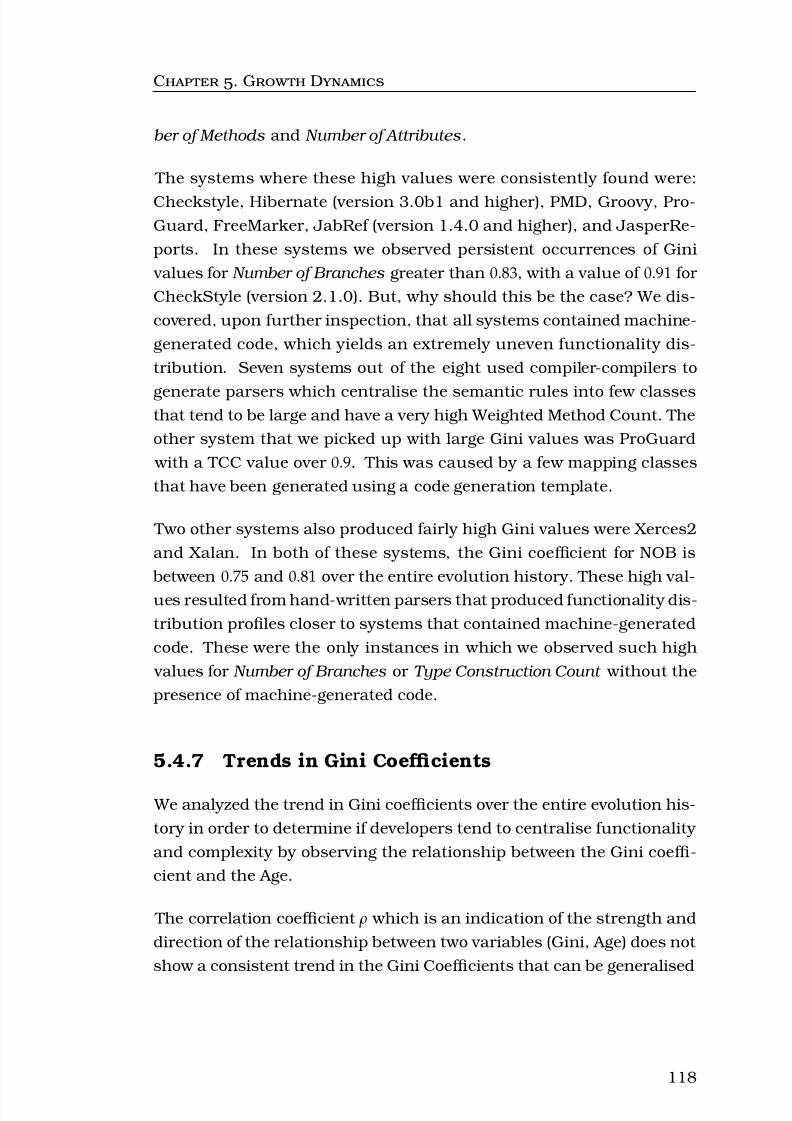
8/8/2019 Rajesh Vasa -- PhD Thesis
http://slidepdf.com/reader/full/rajesh-vasa-phd-thesis 137/252
C . G D
ber of Methods and Number of Attributes .
The systems where these high values were consistently found were:
Checkstyle, Hibernate (version 3.0b1 and higher), PMD, Groovy, Pro-Guard, FreeMarker, JabRef (version 1.4.0 and higher), and JasperRe-
ports. In these systems we observed persistent occurrences of Gini
values for Number of Branches greater than 0.83, with a value of 0.91 for
CheckStyle (version 2.1.0). But, why should this be the case? We dis-
covered, upon further inspection, that all systems contained machine-
generated code, which yields an extremely uneven functionality dis-
tribution. Seven systems out of the eight used compiler-compilers to
generate parsers which centralise the semantic rules into few classesthat tend to be large and have a very high Weighted Method Count. The
other system that we picked up with large Gini values was ProGuard
with a TCC value over 0.9. This was caused by a few mapping classes
that have been generated using a code generation template.
Two other systems also produced fairly high Gini values were Xerces2
and Xalan. In both of these systems, the Gini coefficient for NOB is
between 0.75 and 0.81 over the entire evolution history. These high val-
ues resulted from hand-written parsers that produced functionality dis-
tribution profiles closer to systems that contained machine-generated
code. These were the only instances in which we observed such high
values for Number of Branches or Type Construction Count without the
presence of machine-generated code.
5.4.7 Trends in Gini Coefficients
We analyzed the trend in Gini coefficients over the entire evolution his-
tory in order to determine if developers tend to centralise functionality
and complexity by observing the relationship between the Gini coeffi-
cient and the Age.
The correlation coefficient ρ which is an indication of the strength and
direction of the relationship between two variables (Gini, Age) does not
show a consistent trend in the Gini Coefficients that can be generalised
118

8/8/2019 Rajesh Vasa -- PhD Thesis
http://slidepdf.com/reader/full/rajesh-vasa-phd-thesis 138/252
C . G D
in 9 out of the 10 metrics, the exception was In-Degree Count . In all
metrics except In-Degree Count , the range of ρ values was dispersed
between 0.98 and −0.95. This observation is shown in Figure 5.10 and
the range for In-Degree Count is clearly different from the rest of the
metrics under consideration.
Interestingly, we also observed in the other 9 metrics, the Gini coeffi-
cient values trended up for some metrics, while others moved down in
the same system. There were also very strong positive and strong nega-
tive trends for certain metrics, though not consistently similar across all
systems, for instance in PMD the ρ value for NOB was −0.98 while in Kol-
mafia the value for NOB was +0.89. In approximately 30% of the cases,there was no observable trend, with the ρ value in the range −0.35 to
+0.35 which shows that there is at best a weak relationship. Figure 5.10
provides a box plot that indicates the range and IRQ of correlation co-
efficients for the 10 different metrics under study. As can be seen, the
range of values is very broad and in 5 metrics (ODC,PMC,FOC,LIC and
NOB) the median value was zero.
The In-Degree Count , a measure of popularity was the only one that
consistently showed a positive trend. In 20 systems the ρ value was
greater than 0.8 and in 11 systems the value was in the range 0.55 to 0.8.
3 systems showed a weak relationship ( ρ values of 0.08, 0.22 and 0.33),
while only 3 systems (Struts, Tapestry and Ant consistently) showed a
strong negative trend ( ρ < −0.6).
5.4.8 Summary of Observations
The aim of our study into the nature of growth in software was to un-
derstand if evolution causes growth to be evenly distributed among the
various classes in the software system, or if a certain classes tend to
gain more complexity and size. In order to answer this question, we
studied how the metric data distribution changes over time.
119

8/8/2019 Rajesh Vasa -- PhD Thesis
http://slidepdf.com/reader/full/rajesh-vasa-phd-thesis 139/252
C . G D
- 1
- . 8
- . 6
- . 4
- . 2
0
. 2
. 4
. 6
. 8
1
S
p e a r m a n s C o r r e l a t i o n C o e f f .
IDC PMC NOF TCC ODC NOB NOM SIC LIC FOC
Figure 5.10: Box plot of Gini coefficients correlated with Age
The results of our study show that:
1. Software size and complexity metric distributions are non-gaussian
and are highly skewed with long tails. Developers seem to favor so-
lutions with few large and complex abstractions.
2. The metric distributions of both size and complexity measures, for
any given application change very little between two consecutive
versions. Though the distribution is stable, there are occasional
spikes indicating significant changes do occur. However, the gen-
eral pattern is that once developers commit to a specific solution
approach the organisational preferences are consistent as the soft-
ware system evolves.
3. Systems that contain machine generated code (such as those cre-
ated by compiler-compilers or generated wrapper classes) have a
unique profile and are detectable by Gini Coefficient values over
0.85.
120

8/8/2019 Rajesh Vasa -- PhD Thesis
http://slidepdf.com/reader/full/rajesh-vasa-phd-thesis 140/252
C . G D
4. The popularity of a class is not a monotonic function of its size or
complexity (as captured by our 10 metrics). In other words, large
and complex classes are no more popular than small and simple
classes.
5. The process of software evolution in general causes popular classes
to gain additional dependents and hence become even more pop-
ular.
5.5 Discussion
In this section, we discuss how developers choose to maintain software
systems by interpreting the observations presented in the previous sec-
tion. Specifically, we argue that though the different metrics selected
are strongly correlated, the inconsistency of the strength between dif-
ferent systems warrants the use of different metrics in order to under-
stand the maintenance of a software system effectively. Furthermore,
we discuss the finding of the consistent increase in the Gini Coefficient
value of the In-Degree Count and argue that this observation provides
the empirical support for the preferential attachment model that has
previously been postulated as one of the likely models of growth. We
also present an explanation for the observation of highly stable and
strongly bounded range for the Gini Coefficients and show that the de-
cisions that developers make with respect to how they organise a solu-
tion are highly consistent during the development life cycle. Addition-
ally, we present our interpretation for why developers prefer to construct
and maintain solutions with highly skewed distributions where much
of the functionality is centralised into a few god-like classes. We endthe section with a discussion on the value and applicability of the Gini
Coefficient for identifying releases with significant changes as well as
for detecting the presence of machine generated code.
121
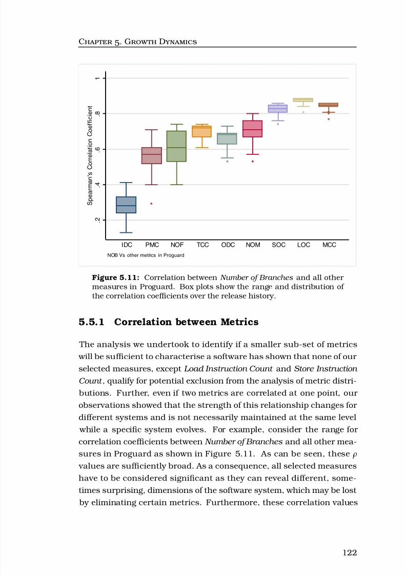
8/8/2019 Rajesh Vasa -- PhD Thesis
http://slidepdf.com/reader/full/rajesh-vasa-phd-thesis 141/252
C . G D
. 2
. 4
. 6
. 8
1
S p e a r m a n ' s C o r r e l a t i o n C o e f fi c i e n t
IDC PMC NOF TCC ODC NOM SOC LOC MCC
NOB Vs other metrics in Proguard
Figure 5.11: Correlation between Number of Branches and all other measures in Proguard. Box plots show the range and distribution of the correlation coefficients over the release history.
5.5.1 Correlation between Metrics
The analysis we undertook to identify if a smaller sub-set of metrics
will be sufficient to characterise a software has shown that none of our
selected measures, except Load Instruction Count and Store Instruction
Count , qualify for potential exclusion from the analysis of metric distri-
butions. Further, even if two metrics are correlated at one point, our
observations showed that the strength of this relationship changes for different systems and is not necessarily maintained at the same level
while a specific system evolves. For example, consider the range for
correlation coefficients between Number of Branches and all other mea-
sures in Proguard as shown in Figure 5.11. As can be seen, these ρ
values are sufficiently broad. As a consequence, all selected measures
have to be considered significant as they can reveal different, some-
times surprising, dimensions of the software system, which may be lost
by eliminating certain metrics. Furthermore, these correlation values
122

8/8/2019 Rajesh Vasa -- PhD Thesis
http://slidepdf.com/reader/full/rajesh-vasa-phd-thesis 142/252

8/8/2019 Rajesh Vasa -- PhD Thesis
http://slidepdf.com/reader/full/rajesh-vasa-phd-thesis 143/252
C . G D
as existing classes gain more size and complexity, that is, they become
relatively wealthier.
In our data set, we found a generalizable and consistent trend only inthe Gini Coefficient for In-Degree Count . The Gini Coefficients for all
other metrics increase in some systems, while in others they decrease.
Our finding shows that the change in distribution of class size and
structural complexity is not a consistent and predictable evolutionary
property. The variability in the Gini coefficients across systems sug-
gests that there are different evolutionary pressures for different sys-
tems and developers respond as needed. However, the stability of the
distribution profiles indicates that a system generally keeps its charac-ter over time — a finding that provides some indirect support for the
Law of Conservation of Familiarity (cf. Section 2.3).
When developers add a set of new classes, these fit within the overall
probability distribution profile as indicated by the minimal change in
the Gini coefficient. Although our observations indicate that the long-
term trend for most Gini Coefficient values cannot be reliably predicted,
there is a high probability that the distribution of size and complexity
between any two consecutive versions are very similar.
5.5.3 Preferential Attachment
We analyzed the trend in the Gini values to answer one of our research
questions – “do large and complex classes get bigger over time?” . If large
and complex classes gain additional volume in terms of code, then they
will grow at a slightly faster rate than the rest of the code base causingthe Gini Coefficient values to increase as software evolves. Our obser-
vations showed a consistent trend in the Gini Coefficient value of IDC,
but none of the other metrics had a sufficiently generalizable trend.
In some systems there was an increase, while in others there was a
decrease in the Gini Coefficient values over time.
Our findings show that popular classes tend to gain additional de-
pendents indicating that, in general, software systems are built incre-
124

8/8/2019 Rajesh Vasa -- PhD Thesis
http://slidepdf.com/reader/full/rajesh-vasa-phd-thesis 144/252
C . G D
mentally, with new functionality constructed on top of existing code.
Though not surprising the real value of our analysis is that it provides
empirical support for the Yule process [210] also known as preferential
attachment growth model. In the simple form of this growth model, as
classes are added, the probability that a class will depend on another
existing class is proportional to the popularity of the existing class [55].
Simply put, popular classes will gain additional dependents causing
their popularity to increase. The preferential attachment model has
been used as one of the explanations for how certain web sites gain
popularity on the world-wide web [16, 209]. An interesting statistical
property of systems that exhibit growth via a preferential attachment
is that the data exhibits a highly skewed distribution and tends to fit a power-law distribution [210].
Many researchers that study software have noted that the In-Degree
Count metric distributions follow a power-law [21,54,55,223,287,299],
and have hypothesised that this distribution arises due to preferential
attachment. That is, they have inferred the potential growth mecha-
nism from the observed outcome. However, although preferential at-
tachment can cause a power-law distribution, it is not the only modelthat can give rise to this category of skewed distributions [48,145]. This
possibility implies that the hypothesis of preferential attachment model
generating skewed In-Degree Count distributions was not fully validated
empirically. Our observations show that, in general, there is an upward
trend in the Gini coefficient for IDC providing empirical support for the
preferential attachment growth model as the most likely explanation for
the observed highly skewed distributions for In-Degree Count metric.
In our data, we observed three systems – Struts, Tapestry, and Ant where the Gini Coefficients for In-Degree Count decreased over time.
Why are these systems different? In order to answer this specific ques-
tion, we had to study the release notes as well as all available architec-
ture and design documentation for these systems.
The developers of Struts and Tapestry performed major restructuring
of the code base and in both cases, abandoned a substantial amount
of the code base during these restructuring phases (more detail is pre-
125

8/8/2019 Rajesh Vasa -- PhD Thesis
http://slidepdf.com/reader/full/rajesh-vasa-phd-thesis 145/252
C . G D
sented in the next chapter). The major rework has caused the Gini co-
efficient values for In-Degree Count to reduce substantially. In essence,
in both of these systems the popular classes were not able to establish
themselves to gain additional popularity.
The Ant Build system was unique in its behaviour as the Gini Coefficient
value for In-Degree Count decreased gradually over time. Furthermore,
there was no evidence of any substantial rework in this system. The rea-
son that the popular classes slowly lost popularity was driven by the
inherent architecture of Ant, specifically how new features were added.
In Ant, new features were typically added into the core functionality via
a plug-in architectural style. The plug-in contained a set of new classesthat provided the needed functionality. Although the plugins rely on
some of the existing core classes, the dependency binding into the core
classes was achieved via external configuration files rather than stat-
ically in Java code. However, since our metric extractor is unable to
process external configuration files to determine dependency informa-
tion, we were not able to fully identify these dependencies. When the
dependency data was checked manually for four consecutive versions
(1.6.4, 1.6.5, 1.7.0 and 1.7.1), we observed a weak positive correlationtrend.
Unlike In-Degree Count , in the other metrics there was no strong gen-
eralizable trend in the Gini Coefficient suggesting that growth models
other than preferential attachment may be at work.
5.5.4 Stability in Software Evolution
We observed in our analysis that Gini coefficients normally change little
between adjacent releases. However, changes do happen and may result
in significant fluctuations in Gini coefficients that warrant a deeper
analysis (see Figure 5.9 showing selected Gini profiles for all releases of
the Spring framework). But why do we see such a remarkable stability
of Gini coefficients?
Developers accumulate system competence over time. Proven tech-
126
8/8/2019 Rajesh Vasa -- PhD Thesis
http://slidepdf.com/reader/full/rajesh-vasa-phd-thesis 146/252
C . G D
niques to solve a given problem prevail, where untested or weak prac-
tices have little chance of survival. If a team has historically built soft-
ware in a certain way, then it will continue to prefer a certain approach
over others. This typical human behavioural trait was originally ob-
served by Milgram [197] who showed that given multiple choices, most
people will avoid selecting the choice which would invalidate their previ-
ous behaviour. Furthermore, this regularity in behaviour is consistent
even at the level of a group [276] (Chapter 14). Although the problem
context and personalities within the group have been shown to influ-
ence how a group behaves, in general, group behaviour is consistent
over time [276]. Moreover, in the context of software development, we
can expect that most problems in a given domain are similar, hence themeans taken to tackle them would be similar, too. Tversky and Kahne-
man coined the term decision frame [285] to refer to this principle in
which decision-makers proactively organize their solutions within well-
established and strong boundaries defined by cultural environment and
personal preferences. Our study suggests that these boundaries man-
ifest themselves also in the software systems.
When developers are making decisions, they weigh the benefits of usinga large number of simple abstractions against the risk of using only a
few, but complex ones in their solution design. Our findings indicate
that developers favor the latter. In particular, we learned (see Figure 5.7)
that the Gini coefficients of most metrics across all investigated systems
assume bounded values. These values mark a significant inequality
between the richest and the poorest. For example, in Spring framework
version 2.5.3 approx. 10% of the classes possess 80% of the Fan-Out
Count wealth (see Figure 5.3).
Another observation we made is that it is rare to see Gini coefficients
greater than 0.8. For example, we noticed that in Struts, a Web applica-
tion framework, the Gini coefficient for In-Degree Count initially moves
beyond this threshold, only to fall back below it within a few releases
(see Figure 5.8). This interesting behaviour reveals that, in order for
software systems to sustain evolution, responsibilities have to be dis-
tributed across abstractions in such a way that developers can maintain
their cohesion, further supported by the lower and upper bounds that
127

8/8/2019 Rajesh Vasa -- PhD Thesis
http://slidepdf.com/reader/full/rajesh-vasa-phd-thesis 147/252
C . G D
System Measure Ver. Gini Explanation
1.01 0.81PMDTCC 1.02 0.73
User interface code refactored into multiplesmaller classes.
2.4 0.44CheckstyleIDC 3.0b1 0.80
Plug-in based architecture introduced.
3.8 0.78ProguardTCC 4.01 0.90
2,500 line obfuscation instruction mappingclass introduced.
1.3 0.75JabRefNOB 1.4 0.91
Machine generated parser introduced.
2.1.7 0.51WebWorkMIC 2.21 0.62
A large utility class and multiple instances ofcopy-and-paste code introduced.
2.0a 0.59Xerces2IDC 2.0b 0.78
Abstract syntax tree node referencingchanged.
1.0.3 0.58JasperReportsPMC 1.1.0 0.69
Significant design approach change with in-troduction of a set of new base classes.
Table 5.4: Sample of observed significant changes to Gini coefficientsin consecutive releases.
appear to define corresponding limits (cp. Table 5.3).
The existence of both lower and upper bounds for Gini Coefficients in
software systems can be viewed as a result of a trade-off developers use
throughout development. Decisions on how to allocate responsibilities
to classes within a system are a product of the application domain, past
experience, preferences, and cultural pressures within the development team. The Gini Coefficient is a potential mechanism for summarising
the outcome of these choices.
5.5.5 Significant Changes
The stability of the Gini coefficient indicates that developers rarely make
modifications to systems that result in a significant reallocation of func-
tionality within the system. Managers can, therefore, use this knowl-
edge to define project-specific triggers both to help detect substantive
shifts in the code base and to ask directed questions about the reasons
for their occurrences. For example, in our study we were able to detect
a major change in the Type Construction Count of Proguard, a Java byte
code obfuscator, between release 3.8 and 4.0 (cf. Table 5.4). A detailed
analysis disclosed that the developers had added a set of large auxil-
iary classes to centralise the obfuscation mapping of instructions — a
change, so significant, as to warrant an appropriate notification to both
128

8/8/2019 Rajesh Vasa -- PhD Thesis
http://slidepdf.com/reader/full/rajesh-vasa-phd-thesis 148/252
C . G D
Figure 5.12: Evolution of Type Construction Count for ProGuard.
internal and external team members. A sample of observed significant
changes in Gini Coefficients is presented in Table 5.4.
Architects often face a situation in which they have to select a third-
party component. They need to consider the desired functional require-
ments as well as project-specific and institutional principles governing
local development practices and styles.
In other words, we need to consider risks arising from mismatches be-
tween existing team habits and newly adapted third-party preferences. Therefore, before a final decision is made, architects should inspect past
or ongoing projects and compare the responsibility distribution profiles
(captured in the respective Gini coefficients). This method focuses on
fitness rather than prescriptive rules to proactively avert emerging de-
velopment risks.
The true benefit of the Gini coefficient is its ability to capture precisely
and summarize changes in both the degree of concentration and the
129

8/8/2019 Rajesh Vasa -- PhD Thesis
http://slidepdf.com/reader/full/rajesh-vasa-phd-thesis 149/252

8/8/2019 Rajesh Vasa -- PhD Thesis
http://slidepdf.com/reader/full/rajesh-vasa-phd-thesis 150/252
C . G D
equilibrium within which software evolution occurs.
The empirically observed nature of software systems is at odds with the
recommendations of how software should be structured. Specifically,some of the guidelines prescribed by Object-Oriented Design Heuristics
[237] as well as rules that are considered to encourage good practice
[136, 161, 178, 179,189].
These design guidelines suggest that developers should construct class-
es with clearly defined responsibilities [303] which are neither too com-
plex nor too big [237]. Though some attempts have been made to quan-
tify high complexity and large classes [61,244] the interpretation of theheuristics has been left as a contextual and hence subjective choice of
the developers.
The design guidelines are fairly broad. However, if the recommenda-
tions are followed, the metric distributions should be less skewed than
observed since complexity and size would be much more equitably dis-
tributed. Although our observations do not imply that developers ac-
tively ignore these recommendations, nor that the recommendations
themselves are incorrect, we still need to reconcile how developers areconstructing software with how they ought to construct software. The
likely explanation for the centralization of complexity and key func-
tionality into few abstractions is that developers tradeoff volumetric
complexity with structural complexity. That is, developers prefer to
deal with a few complex classes rather than a large number of sim-
pler classes. This explanation is supported by research into human
memory in the field of cognitive psychology [12, 13]. These studies into
memory and recall have shown that in general humans working mem-ory works well when the task requires only working with few (less than
10) chunks of information [75].
In the context of object-oriented software development, the chunks of
information are classes and developers will, in general, reduce the num-
ber of classes that they have to hold in their working memory. Specif-
ically, this is likely achieved by ensuring that for a given feature, de-
velopers will implement the functionality by ensuring that the set of
131

8/8/2019 Rajesh Vasa -- PhD Thesis
http://slidepdf.com/reader/full/rajesh-vasa-phd-thesis 151/252

8/8/2019 Rajesh Vasa -- PhD Thesis
http://slidepdf.com/reader/full/rajesh-vasa-phd-thesis 152/252
C . G D
consulting exercise specifically to help understand the nature of code
developed by a third party. This auditing exercise was not part of the
initial scope of this research project. Both software systems were devel-
oped in Java and had an evolution history of a minimum of 4 versions.
When we audited the systems, we used two rules to help us trigger a
broader investigation. The first rule was to look if over the evolution
history the Gini coefficient for any of the metric was outside the upper
boundary of the Inter-Quartile Range for that metric (see Figure 5.7)
as this suggests a distribution that is atypical. The second rule that
we applied was to investigate releases where any of the 10 metrics had
a Gini coefficient value over 0.85. This value occurs only 2.5% of thetime in our data (if we ignore metric, release and system). Essentially
this is a rare occurrence and flags potential machine generated code
(discussed in Section 5.5.8).
In the first system (tax calculation software for large corporations with 5
releases) that we audited applying the above rules, we noticed that the
Gini coefficient for NOB, NOA and TCC was consistently over 0.95 (in all
5 versions available for investigation). Additional investigation showed
that this system contained a large number of stub classes that were
generated from code templates. Interestingly, the stub class generator
was a script developed specifically for this purpose and even though
these stub classes were used extensively their generation technique was
not specifically documented.
The second system that we investigated (phishing site detection engine
with 8 releases) had Gini coefficient values within the IQR. There were
however, two substantial jumps identified as a relative change over 4% between consecutive releases in the In-Degree Count and Out-Degree
Count Gini Coefficient values. These two releases involved major revi-
sions, specifically a reorganisation of the architecture to improve main-
tainability and changes in many classes to improve performance. Unlike
the first system, in the second system, the changes were documented
in the release notes.
Using the Gini Coefficient in both cases identified key aspects of the
133

8/8/2019 Rajesh Vasa -- PhD Thesis
http://slidepdf.com/reader/full/rajesh-vasa-phd-thesis 153/252
C . G D
Figure 5.13: NOB Gini profile for JabRef.
software systems quickly without a deep investigation of the source
code and source repository logs. Our personal experience from the two
audits was that the quick identification of the use of templates to gen-
erate code in the first system helped us identify a key design element
of the solution at the beginning of our audit exercise allowing for more
effective use of our time since we eliminated the need to investigate
approximately 30% of the classes scattered across different packages.
5.5.8 Machine-generated Code
In our study we noticed that certain systems consistently exhibited
Number of Branches Gini values above 0.85. An investigation into those
unusually high values revealed the presence of machine-generated code ,
specifically parsers and expression processors. These parsers typi-
cally contain a few large classes that encapsulate very long methods
with abnormally high algorithmic density caused by many thousands
of branches that use of hundreds of variables. This is caused because
code generators often employ greedy strategies to map a given specifi-
cation to target code.
Systems that contain machine-generated code structures tend to have a
unique distribution profile, where Gini Coefficients tend to be close to 1
134

8/8/2019 Rajesh Vasa -- PhD Thesis
http://slidepdf.com/reader/full/rajesh-vasa-phd-thesis 154/252
C . G D
(see Figure 5.13 showing the Number of Branches Gini Coefficient values
for JabRef). JabRef is a tool that helps manage bibliography databases,
specifically BibTex files. Interestingly, the developers initially used a
hand-written parsers and in RSN 6 introduced a machine generated
parser. The introduction of the machine generated parser for BibTex
files caused the Number of Branches Gini Coefficient value to increase
from 0.74 to approximately 0.91 (see Figure 5.13).
High Gini Coefficient values indicate that these systems have a small
set of very large and complex classes (wealthy in terms of size and com-
plexity). As noted earlier, human developers rarely write code in which
Gini Coefficients for specific measures go past 0.80 as they will find it hard to write and maintain methods with very high algorithmic com-
plexity [74,263]. The ability of detecting and flagging machine generated
code is valuable since it signals the possible need for additional exper-
tise in order to maintain or enhance an existing code base and to meet
strategic objectives.
Interestingly, we did notice a higher Number of Branches value (Gini Co-
efficient around 0.8) in two XML parsers Xerces and Xalan, both of which
contained human written parsers. We determined that they were hand
written by studying repository access logs and comments left within
the code. When machines generate parsers, they create a full set of
classes rather than partially adjusting a few lines to fix defects, this is
visible in the repository logs related to those files. Further, the code
files written by machine use variable names that are alpha-numeric
with the numeric component increasing in value for each new variable
rather than in a human readable form (for example the variables gener-
ated by the machine generated parser take the form jj_123, jj_124,
jj_125 etc.)
Surprisingly, in software with human written parsers, the developers
choose to centralise the functionality of the parser into a few classes
with large and complex methods rather than distributing the complexity
among a large number of classes. Though these classes did not match
the size or complexity of machine generated code, they influenced the
overall distribution sufficiently to cause a higher Gini value.
135

8/8/2019 Rajesh Vasa -- PhD Thesis
http://slidepdf.com/reader/full/rajesh-vasa-phd-thesis 155/252

8/8/2019 Rajesh Vasa -- PhD Thesis
http://slidepdf.com/reader/full/rajesh-vasa-phd-thesis 156/252
C . G D
of wealth.
The results from our study showed that metric distributions have a
similar shape across a range of different systems. These distributionsare stable over long periods of time with occasional and abrupt spikes
indicating significant changes are rare. A general pattern is that once
developers commit to a specific solution approach, the organisational
preferences are stable as the software system evolves.
An unexpected finding of this study was the observation that systems
containing machine generated code have distributions that are signifi-
cantly more skewed. Based on this unique profile we developed a tech-nique that can be used to automatically detect the presence of generated
code — a technique that can greatly aid software comprehension as well
as to assist in software reviews.
Our analysis shows that the popularity of a class is not a function of
its size or complexity, and that evolution typically drives these popular
classes to gain additional users over time. This finding provides em-
pirical support for the Yule process, also known as the preferential at-
tachment growth model. Interestingly, measures of size and structuralcomplexity do not show generalizable pattern. That is, large and com-
plex classes do not get bigger and more complex over time purely due to
the process of evolution, rather there are other contributing factors that
determine which classes gain complexity and volume. Identification of
these factors is an area that we leave as future work.
Given that popular classes in general gain additional popularity in evolv-
ing software, a natural question that arises is – “does this growth in popularity place any pressure on popular classes to change?” Lehman’
Laws of Software Evolution [174] suggest that software systems, due to
their very use, provide evolutionary pressures that drive change. Would
classes due to their popularity also undergo modifications? Although,
this was not an initial research question that we set out to answer in our
study, we added it into our study of the nature of change and discuss
our findings in the next chapter.
137
8/8/2019 Rajesh Vasa -- PhD Thesis
http://slidepdf.com/reader/full/rajesh-vasa-phd-thesis 157/252
Chapter 6
Change Dynamics
It is a widely accepted fact that evolving software systems change and
grow [166]. However, it is less well-understood how change is dis-
tributed over time, specifically in object oriented software systems. The
patterns and techniques presented in the previous chapter permit de-
velopers to identify specific releases where significant change took place
as well as to inform them of the longer term trend in the distribution
profile. This knowledge assists developers in recording systemic and
substantial changes to a release, as well as to provide useful informa-
tion as input into a potential release retrospective. However, the anal-
ysis methods presented in the previous chapters can only be applied
after a mature release of the code has been developed. But in order
to manage the evolution of complex software systems effectively, it is
important to identify change-prone classes as early as possible. Specif-
ically, developers need to know where they can expect change, the like-
lihood of a change, and the magnitude of these modifications in order totake proactive steps and mitigate any potential risks arising from these
changes.
Previous research into change-prone classes has identified some com-
mon aspects, with different studies suggesting that complex and large
classes tend to undergo more changes [20,28,31, 63, 130,177,213,266,
314,318], and classes that changed recently are likely to undergo mod-
ifications in the near future [93, 94]. Though the guidance provided is
138
8/8/2019 Rajesh Vasa -- PhD Thesis
http://slidepdf.com/reader/full/rajesh-vasa-phd-thesis 158/252
C . C D
helpful, developers need more specific guidance in order for it to be ap-
plicable in practice. Furthermore, the information needs to be available
at a level that can help in developing tools that highlight and monitor
evolution prone parts of a system as well as support effort estimation
activities.
The specific research questions that we address in this chapter are:
• What is the likelihood that a class will change from a given version
to the next?
– Does this probability change over time? – Is this likelihood project specific, or general?
• How is modification frequency distributed for classes that change?
• What is the distribution of the magnitude of change? Are most
modifications minor adjustments, or substantive modifications?
• Does structural complexity make a class susceptible to change?
• Does popularity make a class more change-prone?
In this chapter, we address the above questions and present a set of
recommendations that can help developers to proactively monitor and
manage change. These recommendations are derived from a statisti-
cal analysis of change in approximately 55000 unique classes across
all projects under investigation. The analysis methods that we applied
took into consideration the highly skewed nature of the metric data
distributions, something not always properly considered in previous work [18, 19, 27, 28, 38, 93, 150, 177, 241, 255, 272].
The raw data used is this study is available as data files on the DVD
attached to this thesis. Appendix F describes the various data and
statistical analysis log files related to this chapter.
139

8/8/2019 Rajesh Vasa -- PhD Thesis
http://slidepdf.com/reader/full/rajesh-vasa-phd-thesis 159/252
C . C D
6.1 Detecting and Measuring Change
Change is defined1
as a process of transformation — to make the form different from what it is . The first step in understanding change is to
identify the unit of change , specifically, the entity that is undergoing
change. This is important since change can be observed and under-
stood at different levels of abstraction (for example, package/module,
class or method in an object-oriented systems). Since classes are the
abstraction under study in our work, we focused our investigation at
this level.
6.1.1 Approaches for Detecting Change
Detecting if an existing block of code has changed or can be considered
identical to another block of code (i.e., a clone) has been an area of study
for many years [242, 282]. The typical methods applied for detecting
changes are: (a) String matching [72,135,143,243], (b) Abstract-Syntax
tree matching [22], and (c) Metric-based finger print matching [5, 155].
String matching involves splitting a block of code (typically a file) into
lines, sub-strings or tokens and then comparing if these sub-blocks
occur in another file or block of code. The strength of this approach is
its simplicity and variations of this approach have been widely used by
source code version control tools such as CVS [225] and Subversion [53]
to identify if a file (under configuration management) has been modified.
However, this approach has some limitations. String matching does
not analyse change in context of the underlying programming language
semantics which causes it to detect and flag changes even when the
program is semantically identical. For instance, if a method was moved
from the bottom of a class to the top of a class, it would be flagged as a
changed class. Similarly, minor reformatting to improve readability will
also be identified as a change.
The Abstract-Syntax tree (AST) based matching approach relies on the
construction of a syntax tree by parsing a program file and then match-
1Oxford American Dictionary, 2005
140

8/8/2019 Rajesh Vasa -- PhD Thesis
http://slidepdf.com/reader/full/rajesh-vasa-phd-thesis 160/252
C . C D
ing it with another syntax tree. In contrast to the String matching ap-
proach, the Abstract Syntax Tree (AST) based matching is programming
language aware and is able to identify the types of changes more pre-
cisely. Though this approach is comparatively more complex, it has
increasingly been adopted by contemporary IDE’s like Eclipse [73] to
perform an intelligent diff allowing developers to compare two versions
of a class. The AST based matching approach has also been enhanced
to better detect structural changes in object oriented programs by com-
bining it with call graphs analysis [157], and program behaviour anal-
ysis [7].
The metric based finger printing approach involves computing a set of measures from the abstraction that is being monitored and comparing
this set with a set collected after the change has been made. If there
is a difference between these two sets, the abstraction is considered to
have been changed. This approach, depending on the implementation
can be aware of the underlying programming language semantics, es-
pecially if an AST is used to represent the program under analysis. A
key advantage of the metric based approach is its ability in providing
a consistent qualitative distance measure which can be used to deter-mine the magnitude of a change. One such distance measure is the
n -dimensional Euclidian distance measure where the two sets of mea-
sures are treated as the input vectors from which a distance measure is
computed [34,67,155]. The resulting distance falls on the ordinal scale
and only provides sufficient information to permit ordering of changes
by magnitude. That is, we can determine that a specific class has had
a greater level of change than another. However, these measures are
unbounded and hence need to be normalised if they are to be used in a
comparative analysis (discussed in additional detail in the next section).
Change detection algorithms have applications beyond an intelligent
diff of the source code [242]. Variations of these algorithms have been
applied to detect different types of refactoring [288], as well as to iden-
tify duplicate blocks of code (clones ) in a software system [156, 195]
as these have been shown to reduce maintainability [236]. Clones are
in general caused by developers copying and pasting blocks of code,
which is considered a poor programming practice [236]. These clones
141

8/8/2019 Rajesh Vasa -- PhD Thesis
http://slidepdf.com/reader/full/rajesh-vasa-phd-thesis 161/252
C . C D
often make error correction difficult (since an error may be fixed in the
one block of code, yet remain in all of the clones), and also inflate the
size of the code making maintenance harder [236].
Although methods to detect changes have been developed, a compre-
hensive study applying these techniques to understand change and sta-
bility from a statistical perspective has not previously been undertaken.
6.1.2 Our Approach for Detecting Change in a Class
In our study we detect changes using a combination of metrics-based
fingerprint matching and string matching. Our use of metrics to detect
identical classes was inspired by work done by Kontogiannis [154, 155]
who studied programming patterns using metrics to identify potentially
similar blocks of code.
In order to determine change, we start by identifying the class in both
versions under comparison. We establish the identity of a class by using
the fully qualified class name (that is, the class name including the
package name) and checking if that name exists in both versions under comparison. Once identity is established, to determine if a class has
undergone modification, we check if any of the following information
has changed:
1. The class modifiers (i.e., public, private, protected, interface, final
or abstract)
2. The fully qualified name of its direct super class
3. The set of interfaces that this particular class implements (we use
fully qualified names)
4. The name, type and modifiers of all fields
5. The name, signature and modifiers of the methods (the return type
as well as parameter names and types are considered as part of
the method signature)
142

8/8/2019 Rajesh Vasa -- PhD Thesis
http://slidepdf.com/reader/full/rajesh-vasa-phd-thesis 162/252
C . C D
6. The set of classes that this class depends on (defined as lout (n) in
Chapter 4.
7. The set of different absolute count measures computed for theclass (see Table 4.4, Table 4.2, and Table 4.3).
If all of the above information is unchanged for a class in two versions
under comparison, then that class is considered an identical clone and
tagged as unchanged . Although it is possible that some distinctively
smaller subset of the measures (as well as meta data) will suffice to as-
sess weather a class has changed without significant loss of precision,
we adopt the more conservative approach for our analysis and use thefull set.
6.1.3 Identifying Modified, New and Deleted Classes
The set of classes in a given version is N v, and any given version v of a
software system has the following disjoint sets:
• The set of unchanged classes Uv (compared to the previous re-
lease),
• The set of classes that have changed Cv (compared to previous re-
lease), and
• The set of classes that are newly added in this release Av.
Additionally, there also exists the following disjoint sets in a given ver-sion v:
• The set of classes that are deleted in the next release D f v ,
• The set of unchanged classes U f v in the next release, and
• The set of classes that are modified in the next release C f v .
143

8/8/2019 Rajesh Vasa -- PhD Thesis
http://slidepdf.com/reader/full/rajesh-vasa-phd-thesis 163/252
C . C D
The set of changed classes Cv and the set of unchanged classes Uv are
determined by comparing the classes in two releases using the change
detection technique presented in Section 6.1.2.
The set of deleted classes D f v in the next release is determined by com-
paring any given version with the future version (if available) and check-
ing if the fully qualified class name exists in both versions. The set of
newly added classes Av is computed by comparing any given version
with the previous version (if available) and checking if the fully quali-
fied class name exists in that version.
6.1.4 Measuring Change
Once the set of changed classes is established, three different dimen-
sions of change can be computed: amplitude (size of change), periodicity
(frequency of change), and dispersion (consistency of change). These
dimensions were proposed by Barry et al. [17] based on a study into
volatility in software systems where a phase sequence analysis of main-
tenance log data (revision history ) was performed. We based our study
on similar dimensions, however we use release history (see Section 3.1)as our input and hence can not directly apply the method proposed by
Barry et al. [17].
In this study, we use the following definitions for the dimensions of
change — the size of change between two classes is defined as the num-
ber of metrics that differ (i.e., if five different metrics differ in value be-
tween two classes, then the size of change is 5). The modification count
is the number of times a class has been modified since its creation —
this measure is used as the basis for determining the periodicity. Fi-
nally, in order to assess dispersion of change, we measure the propor-
tion of classes in the final version that remain unchanged since creation
as well as the proportion that are modified after being created.
We measure the size, consistency and frequency of change for each class
in our release history (that is, every class in every version). The ratio-
nale for our choices is presented in the next section within the context
of the observations.
144

8/8/2019 Rajesh Vasa -- PhD Thesis
http://slidepdf.com/reader/full/rajesh-vasa-phd-thesis 164/252
C . C D
6.1.5 Measuring Popularity and Complexity of a Class
Once change has been detected and the magnitude assessed, we con-
sider two attributes in order to understand the factors that impact on
the probability of change: the popularity of a class, and the complexity
of a class. A popular class is one that is used by a large number of other
classes. In any development environment, it seems wise to make new
classes depend on stable, reliable parts of the system, rather than on
those that are constantly changing. As a consequence, it seems logical
that new code should depend on existing, proven parts of the system.
If this is the case, popularity should make a class stable. The other as-
pect that is likely to have a close relationship with change is complexity of a class. A complex part, is more likely to have defects [20, 130, 266],
and hence changed as part of a corrective modification. However, the
counter argument is that a complex part should resist change because
developers will avoid these classes to minimize the chance of introduc-
ing new defects.
In our study, we define a class to be popular if it has an In-Degree of 5
or more . The value 5 was selected since, on average, only 20% of theclasses (applying the Pareto principle) in a system have this level of In-
Degree. We use Number of Branches as an indicator of the complexity
of a class.
The set of popular classes is N pv , where N
pv ⊆ N v. Any given version v of
the system has the following disjoint sets of popular classes:
• The set of unchanged popular classes U pv ,
• The set of popular classes that have changed C pv , and
• The set of popular classes that are newly added in this version A pv
6.2 Observations
In this section we present the analysis method as well as the observa-
tions within the context of the key research questions. We start with an
145

8/8/2019 Rajesh Vasa -- PhD Thesis
http://slidepdf.com/reader/full/rajesh-vasa-phd-thesis 165/252

8/8/2019 Rajesh Vasa -- PhD Thesis
http://slidepdf.com/reader/full/rajesh-vasa-phd-thesis 166/252
C . C D
We also gather the following statistics by comparing a version with the
previous version in the release history (if a previous version if available):
uv ratio of classes that are unchanged
cv ratio of classes that are changed
av ratio of classes that are added
The percentages uv, cv, and av are determined as follows:
uv =|Uv|
|N v|(6.2.5)
cv =|Cv|
|N v|(6.2.6)
av =| Av|
|N v|(6.2.7)
and,
uv + cv + av = 1 (6.2.8)
In our input data set, we determined that for any given version v, the
following property (Equation 6.2.9) holds in 80% of the versions:
u f v > c
f v > d
f v (6.2.9)
and the following property (Equation 6.2.10) holds for 75% of versions:
uv > cv > av (6.2.10)
When we look ahead one version, on average across all systems that we
studied, we observe that 75% of the classes are unchanged, 20% are
modified and 5% are removed. When we look back one version to detect
new classes, on average we note that 70% of the classes are unchanged,
22% are modified and around 8% are new classes. Figure 6.2 highlights
147

8/8/2019 Rajesh Vasa -- PhD Thesis
http://slidepdf.com/reader/full/rajesh-vasa-phd-thesis 167/252
C . C D
0%
10%
20%
30%
40%
50%
60%
70%
80%
90%
100%
1 4 6 8 1 0 1 2 1 4 1 6 1 8 2 0 2 2 2 4 2 6 2 8 3 0 3 2 3 4 3 6 3 8 4 0
Release Sequence Number
% C
l a s s e s
Unchanged Modified Deleted
Figure 6.1: Change evolution in the Hibernate framework. This graphillustrates change property captured by Equation 6.2.9.
our observations for Hibernate framework and illustrates the change
evolution.
An interesting observation was that in 12 (30%) systems, at least once
in their lifetime, we noticed the percentage of unchanged classes drop-
ping to zero, indicating that every class in the system was modified be-
tween two releases. Upon closer investigation, we noticed that this was
caused by the developers modifying their package names. In Java, the
standard coding convention is to embed the organisation name within
the package name (for example, org.apache.wicket.Page indicates that this is a project managed by Apache). When projects move between
organisations (or) get adopted by commercial sponsors they tend to re-
name all classes which causes the unchanged class count to drop to
zero. Further, we also had a few instances (25 versions), where de-
velopers renamed some of the packages, but left many with the older
names. When they partially renamed, we noticed that the number of
unchanged classes was mostly under 10%.
148

8/8/2019 Rajesh Vasa -- PhD Thesis
http://slidepdf.com/reader/full/rajesh-vasa-phd-thesis 168/252
C . C D
0%
10%
20%
30%
40%
50%
60%
70%
80%
90%
100%
2 3 4 5 6 7 8 9 1 0 11 1 2 13 1 4 15 1 6 18 1 9 20 2 2 23 2 4 25 2 6 27 2 8 29 3 0 31 3 2 33 3 4 35 3 6 37 3 8 39 4 0 41 4 2 43 4 4 45 4 6 47
Release Sequence Number
% C
l a s s e s
Unchanged Modified New
Figure 6.2: Change evolution in the Hibernate framework. This graphillustrates change property captured by Equation 6.2.10.
Impact of System Maturity
A graphical analysis of our observations (Figure 6.3) suggested that as
software systems mature, the probability that the properties (Equations
6.2.9 and 6.2.10) hold increases. But, is this observation statistically
significant? In order to verify the strength of our observation we used
a non-parametric one-way analysis of variance using age as a proxy
of system maturity. The null hypothesis was that system maturity will
have no impact and both properties (Equations 6.2.9 and 6.2.10) are
just as likely to break in the older systems as it is in the younger sys-tems.
This hypothesis was tested using the Kruskal-Wallis test [279] that
checks equality of population medians among groups. The population
was divided into two groups based on if the property under investiga-
tion holds or not. If age does not have a significant impact then the
population median should be similar for both groups.
149

8/8/2019 Rajesh Vasa -- PhD Thesis
http://slidepdf.com/reader/full/rajesh-vasa-phd-thesis 169/252
C . C D
0
1 , 0
0 0
2 , 0
0 0
3 , 0
0 0
A g e
( D a y s )
N Y
0
1 , 0
0 0
2 , 0
0 0
3 , 0
0 0
A g e
( D a y s )
N Y
Figure 6.3: Box plot of system maturity showing distribution of age(in days since birth) and if the change properties hold. Graph on the
left covers Equation 6.2.9, while the right side graph covers Equation6.2.10.
Kruskal-Wallis equality-of-populations test for the first property (Equa-
tion 6.2.9) resulted in a χ2 value of 29.37 (with 1 degree of freedom), and
for the second property (Equation 6.2.10) resulted in a χ2 value of 24.21
(with 1 degree of freedom). In both cases, the χ2 value is well above the
critical level of 3.84 (1 degrees of freedom ) and hence the null hypothesis
was rejected at a significance level of 0.05.
The Kruskal-Wallis test shows that system maturity has an impact, but
it does not answer a related question – Does the probability that the
stated properties hold increase with age? . That is, as software matures
does the probability of stability increase from the 80% indicated for the
first property? In order to answer this specific question, we constructed
a Logistic model [279] to predict the probability that the change prop-
erties (Equations 6.2.9 and 6.2.10) will hold.
150

8/8/2019 Rajesh Vasa -- PhD Thesis
http://slidepdf.com/reader/full/rajesh-vasa-phd-thesis 170/252
C . C D
. 7
. 7 5
. 8
. 8 5
. 9
. 9 5
P r o b a b i l i t y
0 1000 2000 3000
Age (Days)
. 7
. 7 5
. 8
. 8 5
. 9
. 9 5
P r o b a b i l i t y
0 1000 2000 3000
Age (Days)
Figure 6.4: Probability of change reduces with system maturity.Graph on the left indicates the probability that Equation 6.2.9 holds,
while the right side graph indicates probability for Equation 6.2.10. The probabilities were predicted from the Logistic regression models. Age indicates days since birth.
The logistic model was used here rather than the OLS regression model
since it is specifically designed to handle response variable with di-
chotomous (that is, can be one of two possibilities) outcomes. In our
model we used Age as the explanatory (independent) variable while the
response (dependent) variable was if the change property holds (0 wasused to represent where the property was violated, and 1 was used to
represent where the property holds). The parameters of the model were
estimated using the Maximum Likelihood Estimate (MLE) method and
the probability that the property holds was calculated from the logistic
models for each value of age.
The models that we constructed for both properties showed that Age
was a statistically significant predictor of how strongly the change prop-
151

8/8/2019 Rajesh Vasa -- PhD Thesis
http://slidepdf.com/reader/full/rajesh-vasa-phd-thesis 171/252
C . C D
erties hold. For every one unit increase in Age (that is one day), the
odds that the change property holds increases by a factor of 1.0008
for Change Property 6.2.9, and by a factor of 1.006 for Change Property
6.2.10. The predicted properties are presented graphically in Figure 6.4
and show that as software systems mature, the proportion of code that
is modified reduces.
The key finding is that as software evolves, though classes resist change,
there is a certain proportion that are still modified. Furthermore, our
observations suggest that in general, the number of modified classes
is greater than the number of new or deleted classes. The main appli-
cation of this observation is in effort estimation, since if x new classesare anticipated to be added in the next version our change properties
show that at least x classes will be changed. Though, our findings do
not imply that the new classes cause the change, the consistency of
this observation in our data set suggests that it can be applied as a
heuristic during the planning stage.
The probabilities that the change properties will hold were derived by
using the entire data set of releases, ignoring individual projects. How-
ever, when we apply the break down by project, we noticed that in 7
systems these properties (Equations 6.2.9 and 6.2.10) are violated sig-
nificantly more than expected. For instance, Ant Build System violates
the second property (Equation 6.2.10) approximately 45% of the time,
well over the 25% probability that was identified for the second prop-
erty. Interestingly, apart from Ant, in all other systems the probability
that both properties hold is at least 60%. Though there was no common
and consistent driver across all of these systems, the higher than nor-
mal change pattern can be explained by certain architectural choices(Ant has a plug-in architecture hence new classes can be added with
minimal changes to existing code) and decisions made regarding devel-
opment method (details are presented in section 6.3).
152

8/8/2019 Rajesh Vasa -- PhD Thesis
http://slidepdf.com/reader/full/rajesh-vasa-phd-thesis 172/252
C . C D
6.2.2 Rate of Modification
As noted in the previous section, a relatively small set of classes in
any given version is subject to change. However, how often are these
classes modified? What does the distribution of this modification look
like? In order to understand this better, we investigated the number
of times a class is modified. We ignore the total number of releases
for a project intentionally as it will reveal if there is a common pattern
between systems at an absolute level. For example, we can answer the
question - what is the probability that developers will modify a class more
than 3 times? In essence, we are making the assumption that after
a certain point (say the first few releases) the maturity of a softwaresystem will have a minimal impact on the number of times a class is
modified.
For the analysis, we measured the number of times a class has been
modified since birth across the entire data set (approximately 55300
classes across all projects). In our data, on average 45% of the classes
were never modified once created. However, when the data was an-
alyzed by project, the range of classes that were never modified was between 22% and 63%. For instance, in Saxon only 22% of the classes
were unchanged, while at the other end in Jung and ActiveMQ 63%
of the classes were unchanged after birth. Only considering classes
that have been modified at some point in their life cycle and counting
the number of times that they have been changed, we can observe that,
approximately 60% of the classes are modified less than 4 times (see
Figure 6.5). The range is however fairly broad. In Jung, for example,
90% of modified classes are changed less than 3 times.
Furthermore, though most systems have a similar modification pro-
file (see Figure 6.5), a few systems (Axis, iText, Saxon, Jung and Ac-
tiveBPEL) show up as clear outliers. Axis, iText and Saxon had relatively
higher number of classes that underwent modification, we noticed that
Jung and ActiveBPEL were at the other extreme with fewer classes that
underwent changes. In 33 systems less than 10% of all modified classes
were changed more than 8 times. This suggests that the probability that
a class is modified multiple times is quite low and that this probability
153

8/8/2019 Rajesh Vasa -- PhD Thesis
http://slidepdf.com/reader/full/rajesh-vasa-phd-thesis 173/252
C . C D
0%
10%
20%
30%
40%
50%
60%
70%
80%
90%
100%
1 2 3 4 5 6 7 8 9 10 11 12 13 14 15 16 17 18 19 20 21 22 23 24 25
% C
l a s s e s ( C u m u l a t i v e )
Modification Count
Axis
Azureus
Castor
Checkstyle
Findbugs
Groovy
Hibernate
Jung
Spring
Struts
Webwork
Wicket
Saxon
Xerces
Xalan
ActiveBPEL
iText
Figure 6.5: Cumulative distribution of the modification frequency of classes that have undergone a change in their lifetime. The figure only shows some systems from our data set to improve readability. Systemsthat are considered outliers have been shown with dotted lines
reduces non-linearly, as is shown in Figure 6.5. Further, less than 1%of classes were modified more than 20 times (most systems in our data
set have at least 20 versions) which shows that only a small proportion
of the classes undergo repeated adjustments.
Although there is some variance between systems, most systems in our
data set have a similar profile. The range also shrinks as the modi-
fication count increases. The data range for modification count of 2
is close to 15%, however the range falls to 7% once the modification
count reaches 4 and is less than 3% by the time we consider modi-
fication count of over 10. This consistency across different software
systems indicates that the number of releases in the history of a soft-
ware system has a minimal impact on the number of times a class is
modified.
154

8/8/2019 Rajesh Vasa -- PhD Thesis
http://slidepdf.com/reader/full/rajesh-vasa-phd-thesis 174/252
C . C D
0.0%
10.0%
20.0%
30.0%
40.0%
50.0%
60.0%
70.0%
80.0%
90.0%
100.0%
0 1 2 3 4 5 6 7 8 9 10 11 12 13 14 15 16 17 18 19 20 21 22 23 24 25 26 27 28 29 30 31 32 33 34
Axis
Saxon
Xerces2
Xalan
PMD
Wicket
Jung
ActiveBPEL
iText
Figure 6.6: Number of measures that change for modified classes. x-axis shows the number of measures that have been modified, while the y-axis shows the percentage of classes
6.2.3 Distribution of the Amount of Change
As software evolves, we have observed that there is a proportion of code
that changes, but the number of modifications is minimal. But what
is the magnitude of this change? Is there a typical profile for most
systems, such as the one we observe in the modification frequency?
In order to observe the amount of change, we focus on the classes in
the final version that have been modified at least once in their life cycle.
We then compute the set of measures that have changed between a
class when it was first created and its state in the final version. We usethe final version as the baseline to allow for a qualitative comparison
between versions and also to check if there is a broad pattern that is
independent of system maturity. This high-level approach allows us to
see if there is a common profile across the various systems.
Measuring only the number of metrics that change provides a size change
measure that is bounded (since the total number of metrics that can
change is fixed, in our study at 54 metrics). The bounded nature of
155

8/8/2019 Rajesh Vasa -- PhD Thesis
http://slidepdf.com/reader/full/rajesh-vasa-phd-thesis 175/252

8/8/2019 Rajesh Vasa -- PhD Thesis
http://slidepdf.com/reader/full/rajesh-vasa-phd-thesis 176/252
C . C D
abstract classes or enum declarations. The typical zero distance change
in these classes involves modifications such as reordering of parame-
ters in method signatures, renaming fields, parameters or methods, as
well as changes to type names (return types or dependent types).
In all of the systems that we studied, we have not found an instance
where all 54 metrics have changed. The maximum that we found was
34 changed metric values. However, the set of changed metrics was
different for different classes and systems.
6.2.4 Modified Classes and Popularity
In the previous sections we addressed the probability, frequency and
distribution of change. But, what characterizes the classes that do
change? In particular, does popularity increase the stability of a class?
In order to answer this question, within every release across all systems
in our data set we analysed the proportion of classes that are popular
pv (Equation 6.2.11), against the proportion of all the popular classes
that are modified c pv (Equation 6.2.12). In the following two equations,
N pv is the set of popular classes, C pv is the set of popular classes that are
modified, and N v is the set of classes in version v.
pv =|N
pv |
|N v|(6.2.11)
c pv =
|C pv |
|Cv|
(6.2.12)
In order to ensure sufficient statistical power (in terms of our ability
to compare both samples), we eliminate releases where less than 30
classes have changed [271] (Chapter1). Approximately 20% of the re-
leases in our data set have less than 30 modified classes and these have
been excluded from our data analysis.
157

8/8/2019 Rajesh Vasa -- PhD Thesis
http://slidepdf.com/reader/full/rajesh-vasa-phd-thesis 177/252
C . C D
0.0%
5.0%
10.0%
15.0%
20.0%
25.0%
30.0%
35.0%
40.0%
45.0%
50.0%
1 3 5 7 9 11 13 15 17 19 21 23 25 27 29 31 33 35 37 39 41
RSN
% T y p e s
All
Modified
New
Figure 6.7: Spring In-Degree Count evolution. Proportion of modifiedclasses with high In-Degree Count is greater than that of new or allclasses.
We observed the following property (Equation 6.2.13) holds, for 90% of the releases in our data set:
c pv > pv (6.2.13)
Interestingly, even if we include all of the data, that is, we consider re-
leases where less than 30 classes have been modified, the above prop-
erty hold approximately 75% of the time.
Although, this property holds across all releases, are individual sys-
tems different? Does this property get violated more in some systems?
In order to answer this question, we investigated each system. We ob-
served that in 3 systems (Proguard, Tapestry and Acegi), this property
holds only 50% of the time. These systems appear to be outliers (all
other systems in our data set had at least an 80% probability). Inter-
estingly, in 17 systems, the property holds 100% of the time. That is,
in these systems, the majority of modified classes are popular.
158

8/8/2019 Rajesh Vasa -- PhD Thesis
http://slidepdf.com/reader/full/rajesh-vasa-phd-thesis 178/252
C . C D
In Figure 6.7 we see a chart for that illustrates our observation in the
Spring Framework and shows the proportion of popular classes over the
entire evolutionary history. We can see that the proportion of modified
popular classes is consistently greater than the proportion of popular
classes. Developers ideally would approach a class with high In-Degree
Count with care due to the associated risk of impacting other classes
that rely on the services provided. However, our observations show that
typically, classes with a higher In-Degree Count tend to be modified more
than those with lower In-Degree Count .
In the previous chapter we showed that In-Degree Count and size are not
correlated (Spearman’s rank correlation coefficient across all systems was in the range −0.2 and +0.2). This weak correlation implies that
popular classes are being modified, but not because they have more
code.
6.2.5 Modification Probability and In-Degree Count
The analysis presented in the previous section showed that popular
classes tend to be change prone. Further, for any given class the base-
line probability that it will change in its lifetime is 50%. However, does
this probability of modification increase with an increase in popularity?
In order to answer this question, we constructed a Logistic regression
model where In-Degree Count was the explanatory (independent) vari-
able. The response (dependent) variable was if a class was modified at
least once in its release history (0 was used to represent classes that
were not modified, 1 indicated that a class was modified at least once
in its evolution history). The logistic regression model was constructed by using the set of all classes across all versions of all software systems
in our input data set.
The logistic models that we constructed showed that In-Degree Count
was a statistically significant predictor of modification probability (Like-
lihood ratio χ2 = 599.43 with 1 degree of freedom, p-value was 0.0001).
In our model, for every one unit increase in In-Degree Count , the odds
that the class will be modified increases by a factor of 1.029 (95% confi-
159

8/8/2019 Rajesh Vasa -- PhD Thesis
http://slidepdf.com/reader/full/rajesh-vasa-phd-thesis 179/252
C . C D
Figure 6.8: Probability of modification increases as the In-Degree Count of a class increases. This graph is generated based on predicted
values from the Logistic regression where In-Degree Count is the inde-pendent variable.
dence interval is 1.026 – 1.0319). The predicted probability derived from
the model is presented graphically in Figure 6.8 and shows the prob-
ability that a class will be modified increases as it gains additional de-
pendents.
6.2.6 Popularity of New Classes
We have shown in the previous chapter that the distribution of size
measures are stable as software evolves. As a consequence we know
that overall system size growth is mainly due to the addition of new
classes, rather than growth within existing classes. But, what char-
acterizes new classes? How do new classes compare with existing and
modified classes? Are classes born popular or do they acquire popular-
160

8/8/2019 Rajesh Vasa -- PhD Thesis
http://slidepdf.com/reader/full/rajesh-vasa-phd-thesis 180/252

8/8/2019 Rajesh Vasa -- PhD Thesis
http://slidepdf.com/reader/full/rajesh-vasa-phd-thesis 181/252
C . C D
new classes with that of all classes, we can see (Figure 6.7) that this
proportion is consistently lower than the norm. New classes, therefore,
tend to start out with relatively lower popularity and some of these gain
dependents over time. The observation that in general new classes are
less popular than existing classes is also supported by our finding from
the Gini coefficient analysis in the previous chapter. We stated that the
In-Degree Count gini coefficient in general increases as systems mature
which also shows that new classes do not have the same distribution
profile in terms of popularity as the existing classes — if they did, the
Gini Coefficient would not change.
6.2.7 Structural Complexity of Modified Classes
In the previous section we have shown that the popularity of a class
makes it more change-prone. But, does the internal structural com-
plexity of a class increase the likelihood that a class will be modified?
In this section, we address this question by investigating the relation-
ship between the Number of Branches and change.
When a class is modified, there is a certain probability that the branch-
ing statements are altered. To appreciate if the number of branching
instructions has an impact on the probability of change, we constructed
two logistic regression models. In the first model, Number of Branches
was the explanatory (independent) variable. For the second model, we
used the size normalized Number of Branches as the explanatory vari-
able. The size normalized Number of Branches is a ratio calculated as
the number of branches per bytecode instructions in a class. The size
normalization was applied to identify if size causes a significant distor-tion in the probability of modification. That is, the class is being mod-
ified because it is bigger rather than because it has more structural
complexity. In both models the response (dependent) variable was if a
class was modified at least once in its release history (0 was used to
represent classes that were not modified, 1 indicated class was modi-
fied at least once in its evolution history). The logistic regression models
were constructed by using the set of all classes across all versions of all
software systems in our input data set.
162
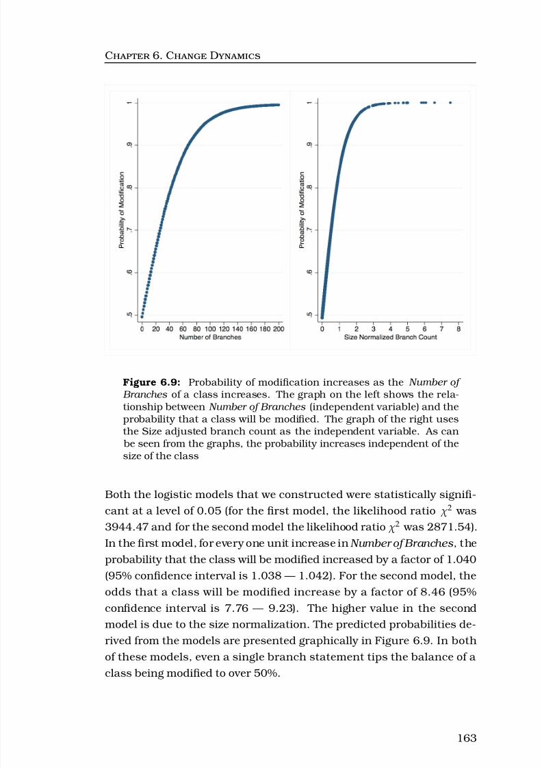
8/8/2019 Rajesh Vasa -- PhD Thesis
http://slidepdf.com/reader/full/rajesh-vasa-phd-thesis 182/252
C . C D
Figure 6.9: Probability of modification increases as the Number of Branches of a class increases. The graph on the left shows the rela-
tionship between Number of Branches (independent variable) and theprobability that a class will be modified. The graph of the right usesthe Size adjusted branch count as the independent variable. As can be seen from the graphs, the probability increases independent of thesize of the class
Both the logistic models that we constructed were statistically signifi-
cant at a level of 0.05 (for the first model, the likelihood ratio χ2 was
3944.47 and for the second model the likelihood ratio χ2 was 2871.54).
In the first model, for every one unit increase in Number of Branches , the
probability that the class will be modified increased by a factor of 1.040
(95% confidence interval is 1.038 — 1.042). For the second model, the
odds that a class will be modified increase by a factor of 8.46 (95%
confidence interval is 7.76 — 9.23). The higher value in the second
model is due to the size normalization. The predicted probabilities de-
rived from the models are presented graphically in Figure 6.9. In both
of these models, even a single branch statement tips the balance of a
class being modified to over 50%.
163

8/8/2019 Rajesh Vasa -- PhD Thesis
http://slidepdf.com/reader/full/rajesh-vasa-phd-thesis 183/252
C . C D
We observed that classes with a higher Branch Count are modified
more than those with lower Branch Count. However, as discussed
in the previous chapter (Chapter 5) class size strongly correlates with
higher Branch Count. But, Number of Branches does not strongly cor-
relate with In-Degree Count , which suggests that classes with complex
code need not be more popular than simpler classes and modifications
spread out beyond popular classes.
6.2.8 Summary of Observations
The aim of our study into the nature of change in software was to informdevelopers where they can expect change, the likelihood of a change,
and the magnitude of these modifications allowing them to take proac-
tive steps.
The observations in our study show that:
• Relatively few classes are modified as a project evolves, class re-
moval is a rare event, and the set of changed classes in general is
larger than the set of new classes in any given version.
• Most classes will be modified at least once in their lifetime, but a
small proportion of classes remain unchanged during their entire
history. Of the classes that are modified, the probability that it
will be modified multiple times is quite low.
• The magnitude of change has a highly skewed distribution. That
is, most classes undergo minor changes.
• Popular and complex classes are more likely to change. Interest-ingly, popular classes do not resist change, on the contrary, pop-
ular classes are more prone to modifications.
• Every class has a raw modification probability of 50%. However,
even a single branch statement or having a single dependent in-
creases the raw modification probability over 50%. Every new
branch increases the probability of modification by 1.04, while
each new dependent increases the probability of modification by
1.03.
164

8/8/2019 Rajesh Vasa -- PhD Thesis
http://slidepdf.com/reader/full/rajesh-vasa-phd-thesis 184/252
C . C D
6.3 Discussion
In the previous section, we summarized our observations. In this sec-tion, we discuss how our findings relate to the maintenance activities
within the development life-cycle and offer an interpretation for the re-
sults.
6.3.1 Probability of Change
We have observed that relatively little code is changed in a software
system as it evolves. This is not only reflected by the small number of classes that change, but also the small amount of change within
modified classes. Our data also reveals that code is even less likely
to be removed than changed. This suggests that developers tend to
resist making substantial changes to the existing code once it has been
released. We can conclude that any code that is released is likely to
resist change.
In all of the systems that we have studied, a good proportion of classes
remained unchanged. This indicates that many abstractions tend to
stay very stable after they are created. The broad range of values for
different systems suggests that this stability depends on the domain
and possibly the development approach as well as the architectural
style that the team has adopted early the development life cycle. Fur-
thermore, the occasional package rename suggests that even with the
availability of tools that can help with refactoring, developers do not
rename or move classes between packages often. Developers seem to
prefer stability in class names, especially once a version of the softwarehas been released.
Our analysis of the relationship between new classes and changed classes
as highlighted by Equation 6.2.10 shows that the set of changed classes
is in general greater than the set of new classes. This finding can be
used during the planning phase for a new version, specifically in im-
proving the effort estimation. For example, if the initial analysis and
design for a new version suggests that there is need for 25 new classes,
165

8/8/2019 Rajesh Vasa -- PhD Thesis
http://slidepdf.com/reader/full/rajesh-vasa-phd-thesis 185/252
C . C D
the change properties identified suggest that there is an 80% proba-
bility that at least 25 classes will be modified. Our observations also
identified that as software matures, these properties (Equations 6.2.9
and 6.2.10) are much more likely to hold. Our results suggest that ma-
turity increases the resistance to change as developers are likely to be
comfortable with the current set of abstractions.
The change properties themselves cannot be directly used to assess the
quality of a software project. Rather, they serve as effective and useful
feedback mechanism allowing managers and developers to understand
the evolution of a software system better and review the code more ef-
fectively. We highlight the value of these properties with two examples which had unusually high violations of the properties.
The first example is the Ant build system, a project that exhibited the
greatest amount of violations (in our data set) of the two change prop-
erties (Equations 6.2.9 and 6.2.10). Our analysis shows that most of
these violations are primarily driven by the plug-in architecture style
used in this software system. Ant is a build automation software sim-
ilar to make [258]. This software was conceptualised and built around
a plug-in based architecture where new build automation tasks can be
developed and added with minimal changes to the existing code. Most
of the enhancements to Ant came as new plug-ins that provided new
build automation tasks. The core of the system is only modified if a large
number of plug-ins are replicating similar functionality. This plug-in
architecture allows developers to create and add new classes without
requiring many changes in the existing code base. This modular archi-
tectural style and the domain of the application in effect meant that in
most new releases, there was a greater proportion of new classes com-pared to modified classes (violating the change properties at a greater
rate than expected).
The second example is Struts, another project that also had a large
number of violations for the change properties (nearly 50% of the re-
leases). An investigation into the release notes and source code of Struts
shows that changes can be attributed to the developers rewriting large
parts of the codebase twice. The first complete re-write used a small
166

8/8/2019 Rajesh Vasa -- PhD Thesis
http://slidepdf.com/reader/full/rajesh-vasa-phd-thesis 186/252
C . C D
portion of the code from the previous versions. The second re-write
abandoned much of the code base and started on top of another open-
source project. This level of fluctuation, and continuous change effec-
tively meant that developers did not have sufficient time to increase the
maturity of the project as it was consistently undergoing substantive
changes.
Although a higher degree of violations of these change properties does
not imply a poor quality software system, consistent and repeated vi-
olations can indicate an unusual phase within the project which may
required additional attention or appropriate documentation to properly
communicate the state of the project to all stakeholders. This type of summarised information is often masked in software project due to the
large volume of changes that take place, and because of a lack of em-
pirically derived heuristics.
6.3.2 Rate and Distribution of Change
Modifications are unavoidable as systems are maintained. However,
very few of the classes tend to experience a high level of modification.
Of the classes that have changed, most have been touched a few times –
only a small proportion is modified several times. This modification pro-
file is very similar in all systems under analysis, suggesting that most
classes in a system tend to reach a stable state very quickly. Combined
with our earlier observation that a good proportion of code is never
touched between releases, this suggests that development teams tend
to create a stable set of abstractions very quickly. Our findings provide
further support to a similar conclusion reached by Kemerer et al. [148] based on an analysis of maintenance logs.
Although our approach does not reveal the actual amount of code that
has changed, it provides us with a broad indicator. One of the systems
that has resisted changes was Wicket, a web application development
framework. Interestingly, the rate of modification in Wicket was close to
many other systems. However, the observed distribution of these mod-
ifications suggests that most of the changes were minor fixes. At the
167

8/8/2019 Rajesh Vasa -- PhD Thesis
http://slidepdf.com/reader/full/rajesh-vasa-phd-thesis 187/252
C . C D
other end, we have Saxon which shows up as a clear outlier in terms
of the rate of modification as well as the distribution of these modifi-
cations. As evident from the data, the developers of this system made
frequent changes, many of which are substantial. Two other systems
had a similar pattern: iText and Axis. But, why was this the case? We
consider this question in further detail in Section 6.3.6.
6.3.3 Popularity of Modified Classes
In the previous sub-sections we argued that developers construct a sta-
ble set of abstractions early in the development life-cycle and that they undertake actions to reduce the size and frequency of these changes as
they prefer stable classes. In this section, we consider our observation
that classes that are popular tend to be change-prone. This observa-
tions is suggestive of Lehman and Belady’s first Law of Software Evo-
lution which states that systems that are used will undergo continuing
change [168, 175]. In our study we see that classes that are heavily
used, i.e., that have high In-Degree Count, are more likely to undergo
change.
This observed popularity of modified classes does not square well, how-
ever, with Martin’s Stable Dependencies Principle [189] which states
that: “The dependencies between components in a design should be in
the direction of the stability of the components. A component should
only depend upon component that are more stable than it is.” On the
surface, the principle appears sound: to improve the overall stability of
our system, we should make new things depend on stable and mature
components. Unfortunately, our new interpretation of Lehman’s Law of Continuing Change suggests that the very fact of depending on a stable
component will make it less stable.
This leads us to question Martin’s popular Instability measure, which
essentially considers an abstraction to be maximally stable when it has
only incoming dependencies and no outgoing dependencies, and max-
imally unstable when it has only outgoing dependencies. Martin’s rea-
soning is based on “stable” meaning “not easily moved” [189]. However,
168

8/8/2019 Rajesh Vasa -- PhD Thesis
http://slidepdf.com/reader/full/rajesh-vasa-phd-thesis 188/252
C . C D
this measure confuses stable with inflexible (“unwilling to change or
compromise”2). A more usual definition of stable is “not likely to change
or fail” (op. cit.). In this case what Martin calls stable we consider to be
unstable , and vice versa.
It is commonly accepted that one should build new software on top of
stable abstraction, that is, on mature components with low rates of
change. This leads, however, to the paradox that by relying on stable
components, we increase their popularity, and thus cause them to be-
come less stable. In effect, this suggests that Lehman and Belady’s
laws of evolution also apply to some degree at a micro-scale: a class
that is used will undergo continuing change or become progressively less useful . For instance, consider the String class (java.lang.String) in the
Java environment which would be expected to be maximally stable due
to its extensive use. But it has consistently changed. The String class
is a popular class that had 30 methods in the first version of Java re-
leased in late 1996, the class in the latest stable build (Java 1.6) has
65 methods and was modified to correct a number of defects and to
provide new functionality such as Unicode support and regular expres-
sion parsing. Though, there is a tendency in popular classes to change,there is likely to be an upper boundary to the external pressures that
drive a classes to change, as developers will want to minimise the po-
tential ripple impact from each change.
Our analysis indicates that there is a very strong probability that pop-
ular classes are less stable. However, in our data we encountered three
outliers — JabRef, Proguard and Acegi where popular classes were just
as likely to be modified as non-popular classes. Despite an exploratory
analysis into each of these systems, we were not able to identify a com-mon driver that can explain our observation. This indicates that our
finding of popular classes being less stable has a strong probability of
occurring, but we cannot yet generalise it into a universal principle with
well defined constraints.2Oxford American Dictionary, 2005
169

8/8/2019 Rajesh Vasa -- PhD Thesis
http://slidepdf.com/reader/full/rajesh-vasa-phd-thesis 189/252
C . C D
6.3.4 Popularity of New Classes
We have seen that the distributions of size and complexity remains sta-
ble, hence it cannot be that growth mainly occurs in existing classes,
but rather in the creation of new classes. But where does this growth
occur — do developers build on top of the existing code base, or do they
tend to build features as components that are added into a software
system?
Since new classes have lower than average In-Degree Count , it seems
clear that growth is on top of existing classes. It is highly unusual for a
new class to have high In-Degree Count , so there must be little growth below classes of the existing system. This finding is also supported by
the Gini coefficient analysis that shows that, in general, the Gini value
of In-Degree Count tends to increase as software matures, suggesting
that as new classes are added they tend to make use of existing classes
hence increasing their popularity. Further, since open-source projects
are known to be developed in an incremental and iterative fashion, our
observations are consistent with the notion that these systems are built
bottom-up, rather than top-down.
6.3.5 Complexity of Modified Classes
We have observed that classes that are modified tend to have a higher
Branch Count than the ones that remain unchanged. Why is this the
case?
Research into defect-prone classes [31, 213, 318] suggests that com-plex abstractions will tend to have more defects. Our observation that
complex classes attract a higher proportion of modification is consis-
tent with the fact that complex classes tend to have more defects and,
therefore, are likely to undergo more modifications as the defects are
corrected. Our observations are incomplete, however, since we have
not analysed the defect data that will allow us to state that changes to
complex classes are principally concerned with correcting defects. Fur-
thermore, it is reported that corrective changes account for only 21% of
170

8/8/2019 Rajesh Vasa -- PhD Thesis
http://slidepdf.com/reader/full/rajesh-vasa-phd-thesis 190/252
C . C D
changes [26], so we cannot conclude that defects are the main reason
for change.
A class that changes is likely to have higher In-Degree Count and higher Branch Count. Simply put, complex classes have a higher probability of
change . Furthermore, this probability increases with the complexity of
the class.
6.3.6 Development Strategy and its Impact on Change
In our data set, three systems stand out as clear outliers: Saxon XML
processor, Axis web services library and iText PDF generation library.
All of these systems exhibited above average change both in terms of
the frequency as well as the magnitude. But, why should this be the
case? Is there a common shared trait?
It turns out that all three systems have one common attribute — they
were all built to satisfy well defined industry standards. Saxon and
Axis implement W3C (World Wide Web Consortium) standards for XML
and Web services, respectively. The iText library attempts to satisfy the Adobe PDF specification. Saxon and iText are currently supported
by commercial (for-profit) organisations, while the Apache consortium
handles the Axis project (Apache is a non-profit organisation that man-
ages a large number of open source projects, including the popular
Apache Web server).
An inspection of the architecture documentation, discussion boards as
well as release notes revealed a consistent theme in all three systems.
In these systems developers made a choice early in the life cycle to incre-
mentally satisfy the specifications, rather than define a software system
that completely implements the standards as elaborated in the speci-
fications. In addition, the developers enhanced their software systems
as the specifications themselves were expanded and amended. Inter-
estingly, in these three systems developers did not create well defined
functional components early in the life cycle. The functional compo-
nents gained coherence and a clear responsibility over time. For in-
171

8/8/2019 Rajesh Vasa -- PhD Thesis
http://slidepdf.com/reader/full/rajesh-vasa-phd-thesis 191/252
C . C D
stance, in Saxon, the developers choose to implement both compile-
time and run-time handlers for XSL-T instructions in the same compo-
nent [144], they also share memory mapped data structures among dif-
ferent components, increasing the inter-dependencies, which has been
shown to increase certain types of defects [130]. Unfortunately, the ex-
act rationale for these choices in Saxon has not been explicitly stated
(our inference is that the choice to merge compile-time and run-time
handlers in Saxon may have been motivated by a desire to improve the
performance).
The architecture guide provided with Axis [11] states that most modules
are not functionally separated and attempt to provide a diverse rangeof functionality, this tight coupling is noted by the developers as an
known concern that needs to be addressed in later releases [11]. The
developers of Axis, interestingly, do suggest a potential solution that can
address the coupling issue in the architecture document [11] but these
recommendations have not been implemented (at time of analysis). The
decisions that the iText team made with respect to compiling are similar
to choices made for Axis and Saxon as inferred from the change logs and
release notes [128].
Another aspect common in iText and Saxon was the choice made by the
developers to build their own collections data structures (such as a List,
Map and Queue) that underwent many changes when they were ini-
tially introduced into the code base. Comments provided in the source
code suggest that the motivation for creating their own collections data
structure was to improve performance. It is possible that at the time
of development the developers did not have access to reliable and ma-
ture high-performance collections classes such as those that exist freely now like GNU Trove [280] and the Google collections framework [107].
Though, reliable high-performance collections libraries now exist the
developers have left their original data structures and algorithms in-
tact.
In iText, Saxon and Axis developers made a number of incremental mod-
ifications. Unfortunately, without an underlying architecture and de-
sign that allowed them to incrementally meet the specifications, they
172

8/8/2019 Rajesh Vasa -- PhD Thesis
http://slidepdf.com/reader/full/rajesh-vasa-phd-thesis 192/252
C . C D
had to modify many classes. The developers, in effect, had to make
changes in a number of classes in new versions as they attempted to
adhere to the standards incrementally. Furthermore, the lack of co-
herent reusable components and libraries, also meant that they had
to improve existing classes rather than upgrade external libraries and
components.
To ensure completeness, we investigated two other systems in our data
set that share a similarity with iText, Saxon and Axis in terms of their
functional domain. The two systems were, Xerces-2 XML processor and
Xalan XSL-T processor. Both these products also satisfy standardised
XML technology specifications developed by W3C. Interestingly, theseprojects made very different choices at the start of their life cycle. The
Xerces-2 project was a complete re-write of the Xerces-1 platform, how-
ever, for the new build, developers satisfied most of the core specifica-
tion in an initial release rather than via incremental refinement. Fur-
ther, based on the experience gained from earlier attempts, the Xerces-2
developers built a modular architecture that allowed them to make in-
cremental adjustments [309] to changing specifications, but the bulk
of the code remained stable. The Xalan project did not have a previousrelease and knowledge base to build on top of [307]. The development
team, however, chose to create a highly modular architecture with well
defined functional boundaries that permitted incremental refinement
and the ability to replace libraries and components [308]. They also
relied on a number of existing stable libraries to provide common func-
tionality (unlike iText and Saxon where developers built many key data
structures and algorithms). The change analysis data suggests that
these choices have helped the team as they evolve and adapt the sys-
tems.
The development strategy and choices made by the developers has an
impact on the change profile. Despite the type of approach taken, all
five systems (iText, Saxon, Axis, Xerces-2 and Xalan) have continuously
evolved, potentially satisfying user needs. However, our study suggests
that when attempting to match formal standards, a modular architec-
ture built after a careful analysis of the entire specification can help
reduce the frequency and magnitude of changes. The strategy of us-
173

8/8/2019 Rajesh Vasa -- PhD Thesis
http://slidepdf.com/reader/full/rajesh-vasa-phd-thesis 193/252
C . C D
ing a loosely coupled modular architecture has been considered ideal
in the literature on software design [257], and our observations provide
further empirical evidence to support the benefits of this strategy.
6.4 Related work
Change in software has been a subject of study by a number of other
researchers and in this section we present key related work to place our
own work in context.
Kemerer and Slaughter studied the profile of software maintenance infive business systems at the granularity of modules by analysing main-
tenance log data. The business systems were closed source and not
developed using object oriented programming languages. Kemerer et
al. conclude that very few modules change frequently, and those that
do are considered to be strategic [148]. Interestingly, our findings are
similar, even though our analysis is based on release history and Open
Source Systems developed using an object oriented programming lan-
guage. The commonality in finding suggests that developers approachsoftware change carefully and tend to minimise them as much as pos-
sible, independent of the licensing and development method used.
Similar to our work, Capiluppi et al. have analyzed the release history
of a number of Open Source Systems [35, 39 – 41] with an intention of
understanding if developers will undertake anti-regressive work, i.e.,
make changes to reduce the complexity of a certain module and hence
improve maintainability. Their studies mainly focused at a macro-level,
in particular on relative changes in the code size and on complexity at a module level [41] as well as the influence of the number of developers on
the release frequency [39]. Their conclusions were that in Open Source
Projects, relatively little effort is invested in anti-regressive work. In our
study we found that developers minimize the frequency and magnitude
of change, and the abstractions that do change tend to be popular or
complex. Interestingly, if developers spend little effort on anti-regressive
work, then it implies that the typical modification is to create new fea-
tures or correct defects.
174

8/8/2019 Rajesh Vasa -- PhD Thesis
http://slidepdf.com/reader/full/rajesh-vasa-phd-thesis 194/252
C . C D
A recent study into change by Gîrba et al. showed that classes that have
changed in the past are also those most likely to change in the future.
They also showed that these classes were the minority [92]. In related
and earlier work, Gîrba et al. have tested the hypothesis that classes
that have changed in the past are likely to change in the future [94].
The reliability of this measure of “yesterday’s weather” seems to vary
according to the “climate” of a software project. Gîrba et al. have also
studied the relationship between change and developers [95]. Addition-
ally, Girba et al. in their studies tag a class as having changed if meth-
ods were added or removed. They also identify change at the method
level by observing a change in the number of statement and the cyclo-
matic complexity. In our study, we used a larger set of properties todetect change and hence are able to identify more fine grained changes.
Rather than modeling and understanding the nature of change, their
goal was to understand which developers are most knowledgeable about
different parts of an evolving system.
Another arc in the study of change has been the area of understand-
ing co-change, where the assumption is made that certain groups of
classes or modules change together [85] because related features aregrouped together. This assumption was supported by research under-
taken by Hassan and Holt who analyzed many Open Source projects
and concluded that historical co-change is a better predictor of change
propagation [113]. This observation is also supported by Zimmerman et
al. [319,320] which led to the development of tools [315] that can guide
developers to consider a group of classes when they modify one class.
Our study however, aims at understanding the statistical properties of
post-release change and inherent properties of a class that might lead
them to change. The properties that we identified can improve project
plans and help during iteration retrospectives, rather than being able
to directly guide developers about potential co-changing classes. Fur-
thermore, Gall et al., Hassan et al., and Zimmerman et al. relied on the
revision history in their studies, and identify change during the devel-
opment phase. We however, investigated the release history and hence
are able to provide a post-release change perspective.
175

8/8/2019 Rajesh Vasa -- PhD Thesis
http://slidepdf.com/reader/full/rajesh-vasa-phd-thesis 195/252
C . C D
Lanza et al. introduced the Evolution Matrix [163] as a means to visu-
alize the evolution of object-oriented software, with the emphasis on re-
vealing patterns of change. Though they are unable to establish which
specific parts of the system are likely to change, their visualisation ap-
proach provides a good overview for developers when they retrospec-
tively audit the evolution of a project in order to better understand the
history and make improvements for the future. More recent work in
evolution visualization [1, 164, 298] has aimed to highlight changes to
the design structure of a software system based on thresholds for met-
ric values at various levels of abstraction (for instance, class or package
level). Our work is slightly different in that we provide statistical prop-
erties of change. Given the additional information in our study, the visualisation tools can incorporate the change properties that we have
identified in order to highlight versions where unusual changes have
taken place.
Koru et al. [109] proposed a tree-based classification technique to iden-
tify change prone classes. Based on an investigation of two Open Source
software systems (KOffice and Mozilla browser) they found that large
classes tend to change more than smaller classes, i.e. size is an ef-fective predictor of change. They also propose a tree based classifica-
tion model to identify change prone classes. The classification method
relies on cyclomatic complexity (similar to Number of Branches in our
study), Lines of code and average change count (per class) in order to
determine which classes may change in the future. In our work, we
show that the probability of change increases with an increase in Num-
ber of Branches . A strength in our study is the size of the underlying
data set from which we base our conclusions. Interestingly, Koru et al.
use the average change count in their predictive model, but the aver-
age values computed may need some additional adjustment to improve
the effectiveness of their approach because we noticed a highly skewed
distribution for magnitude and frequency of change. An additional dif-
ference between our study and the one undertaken by Koru et al. is in
the method used to compute change count. We calculate this value by
analysing the release history, however Koru et al. extract change count
information by analysing revision history (i.e. parsing CVS log files).
176
8/8/2019 Rajesh Vasa -- PhD Thesis
http://slidepdf.com/reader/full/rajesh-vasa-phd-thesis 196/252
C . C D
A study by Bieman et al. [28] examined 39 versions of a single indus-
trial object-oriented software system that evolved over a three year pe-
riod. In this study they investigated the relationship between design
patterns, other design attributes, and the number of changes. Bieman
et al. found a strong relationship between the size of a class and the fre-
quency of changes, that is larger classes were changed more frequently.
This finding fits well with the logical expectation of change, in that larger
classes should change more frequently since there is a larger amount
of code and hence the probability of change increases with size. The
more unexpected and interesting finding in the study was however the
findings that: (a) classes that participate in design patterns are in fact
more change-prone, and (b) classes that are reused the most throughinheritance hierarchies are also change-prone.
More recent work by Aversano et al. [10] and Di Penta et al. [68] based
on empirical investigation of evolution in 3 Java software systems (both
studies used the same data set) arrived at similar conclusions suggest-
ing that classes that participate in design patterns tend to be change-
prone. The findings from the study by Bieman et al., Aversano et al.
and Di Penta et al. complement our own observations. Our study, how-ever, is more specific, in that we show that popular and complex classes
tend to be change-prone rather than be restricted to purely classes that
participate in design patterns or inheritance hierarchies. Additionally,
in contrast to the studies by Aversano et al., Bieman et al. and Di Penta
et al. that focused on a few software systems, we have undertaken a
larger-scale longitudinal study.
Khomh et al. [149] undertook a change-based study investigating 2
Java software systems. They show that classes with code smells aremore change prone than others. The term “code smell” is suggestive
of poor quality in some aspects of the source code, and these smells
are conjectured to negatively impact on the software maintenance ac-
tivities [81]. Khomh et al. identified changes by analyzing the revision
history (source control log files), and then checking if the modified code
exhibited any of the 29 different code smells that they considered to
be representative of poor quality. They conclude that classes with code
smells were more likely to be changed. In their study, one of the code
177

8/8/2019 Rajesh Vasa -- PhD Thesis
http://slidepdf.com/reader/full/rajesh-vasa-phd-thesis 197/252
C . C D
smells that they consider is related to excessive complexity within a
class (computed as the sum of method cyclomatic complexities [190]).
In our work, we use the Number of Branches (NOB) as the measure of
structural complexity within a class. The NOB metric that we use can
be considered to be equivalent to the cyclomatic complexity metric used
by Khomh et al. since both metrics are based on the same underlying
measure (see the NOB metric definition in Chapter 4). The findings by
Khomh et al. are similar to our own conclusions with respect to the
structural complexity of a class suggesting that structurally complex
class are change-prone during development, and post-release. We also,
identified a consistent relationship between popularity and probability
of change which was not considered within the work by Khomh et al..
In a recent study, Capiluppi et al. [36, 37] investigated the value of sta-
bility at predicting reuse of a software module (identified as a set of
files within a source code folder) by studying evolution in 4 long-lived
open source software systems. Capiluppi et al. argue that highly sta-
ble modules are good candidates to be tuned into independent reusable
modules. Capiluppi et al. measured stability by using Martin’s Insta-
bility Metric [189] which uses the coupling of a module (similar to theIn Degree and Out Degree count in our work) as the basis for calcu-
lating the stability. However as discussed in Section 6.3.3, Martin’s
instability metric does not measure actual stability of an abstraction
over time and hence cannot be considered to be a direct measure of
actual change. We also did not find any rigorous longitudinal studies
that have shown the relationship between Martin’s instability metric
and actual changes that take place within a module. In contrast, our
work shows that the new dependants place additional pressure on a
class increasing the probability of change to satisfy new clients.
A key distinction from our own study and that by Capiluppi et al. [36,37]
is the level of abstraction used in the study. We focus on changes at the
class level, while Capiluppi et al. study modules. Although, the level of
abstraction used in our study is different, a module can be treated as
a set of related classes. Therefore, if a set of classes within a module
change, we can considered the module to have changed as well and
hence our findings are likely to be similar at the module level as well.
178

8/8/2019 Rajesh Vasa -- PhD Thesis
http://slidepdf.com/reader/full/rajesh-vasa-phd-thesis 198/252
C . C D
However, a serious investigation of change at higher level of abstraction
remains to be done and we intend to consider it in future work.
6.5 Limitations
In order to place our study in context, we highlight some of the known
limitations of our approach in addition to our findings.
The change detection method used in this work may miss a small set
of classes if the change is not measurable in the metrics under con-
sideration. The accuracy can be improved by adding further metricsand additional aspects like a comparison of the call graph. The value
of this additional complexity remains as a topic for consideration in our
future work. Furthermore, our distance measure compares the initial
version of a class to the final version. This method will miss edits where
a class is modified and returned back to its original shape, as seen by
our change detection technique. This limitation can be addressed by
computing a distance measure incrementally. As a consequence, the
analysis approach will need to be adjusted to take into considerationthe way the metric information is being collected.
Our method of computing modification misses classes that have been
renamed; they will be considered as a deletion (in the earlier version)
and an addition (to the later version). However, of the few classes that
are deleted (less than 4% in general), a subset might be class renames.
We checked if a class has indeed been renamed manually in 300 ran-
domly selected instances. Less than 5% of the classes that we checked
can be considered refactored with a name change. Based on this obser- vation, the benefit from using a complex algorithm to detect renamed
classes is likely to have at best a minimal overall impact and our overall
conclusions and recommendations will still hold.
We have also not investigated in depth why changing classes have higher
than normal In-Degree Count . We speculate that the introduction of
new clients creates the need for adaptations. Other possibilities are
that (i) new clients introduce new requirements, but that suggests new
179

8/8/2019 Rajesh Vasa -- PhD Thesis
http://slidepdf.com/reader/full/rajesh-vasa-phd-thesis 199/252
C . C D
growth in existing classes, which we did not consistently find, or (ii) new
clients exercise existing classes in new ways, thus uncovering previous
unknown defects. Further work is needed to discover which, if any of
these hypotheses is valid.
6.6 Summary
Change in software systems is unavoidable as they are adapted to meet
the changing needs of the users. Our study shows that when we look
at the latest version of a given system, around a third (or more) of the
classes are unchanged in their lifetime. Of the modified classes, very few are changed multiple times, and the magnitude of change is small
suggesting an inherent resistance to change. These findings show that
maintenance effort, which is considered to be a substantial proportion
of the development effort (post initial versions) is spent on adding new
classes. In the absence of a substantial architectural shift or a rewrite
of the system, much of the code base resists change. Furthermore,
efforts to base new code on stable classes will inevitably make those
classes less stable as they need to be modified to meet the needs of thenew clients.
In the next chapter, we discuss the implications arising from our obser-
vations. Specifically, we consider how our findings relate to the Laws
of Software Evolution, and how our work can help improve software
development practices.
180

8/8/2019 Rajesh Vasa -- PhD Thesis
http://slidepdf.com/reader/full/rajesh-vasa-phd-thesis 200/252
8/8/2019 Rajesh Vasa -- PhD Thesis
http://slidepdf.com/reader/full/rajesh-vasa-phd-thesis 201/252

8/8/2019 Rajesh Vasa -- PhD Thesis
http://slidepdf.com/reader/full/rajesh-vasa-phd-thesis 202/252
C . I
ity, that is, because there are a larger number of abstractions that de-
velopers have to deal with over time. However, when we consider the
distribution of size and complexity metrics, we notice that the distribu-
tion of all measures fall within a tight boundary (see Chapter 5). In any
given software system, though there is variation, the overall consistency
in the shape suggests that developers either explicitly or implicitly take
correction action in order to maintain the overall distribution of the
size as well as complexity. The only material increase in complexity at
the system level is not a consequence of complexity of a certain set of
classes, but rather due to the size of the system as a whole and increase
in the absolute number of complex classes.
Our observations related to complexity introduce uncertainty in inter-
preting the law of Increasing Complexity . The law as stated suggests
that complexity increases unless effort is put into reducing it, that is,
it implies that complexity can be managed or reduced . In our study, we
find that (i) there is an absolute increase in the total number of classes,
and (ii) developers either intentionally or otherwise manage to contain
the distribution of complexity between the various classes. These find-
ings lead us to argue that although the distribution of complexity can be managed, the volumetric complexity that arises because of the size
of the system cannot be reduced without a corresponding reduction in
functionality (assuming a competent development team).
Feedback and Regulation
The third law, Self Regulation states that evolution is regulated by feed-
back [166]. We do not collected direct quantitative data related to feed- back. However, the bounded nature of Gini Coefficients across multiple
software systems provides indirect support for this law. Feedback can
be caused by different drivers. For instance, developers will get feed-
back from a set of classes that are too large or complex, especially if
these classes are defect prone. Feedback can also be driven by team
dynamics as well as the cultural bias (strong team habits) that influ-
ence how software is constructed. Hence, it is likely that there are
potentially multiple sources of feedback at work in order to regulate the
183

8/8/2019 Rajesh Vasa -- PhD Thesis
http://slidepdf.com/reader/full/rajesh-vasa-phd-thesis 203/252
C . I
overall structure and shape of the distribution. We found no evidence
that developers actively measure the metric distribution and aim to fit
within it, as there is no traces of this type of behaviour in the change
logs, development process documents or release notes that we studied.
The interesting aspect is that developers have no direct knowledge of
the overall distribution, yet the set of choices they make ensure that the
overall profile is highly consistent. This suggests that feedback operates
at the local level rather than at the system level. That is, developers no-
tice that a certain class is too complex and take steps to correct that.
Similarly, refactoring efforts [81] in most cases are likely to be choices
made with local information.
This behaviour of developers relying on localised feedback is indicative
of software maintenance being a stochastic process that generates an
emergent pattern when observed at the system level. We define emer-
gence in this context as a process that drives a system to acquire a
spatial, functional and temporal structure without specific directed in-
terference from outside. By specific, we mean that the structure or
functioning is not the result of directed and planned actions, rather
the system achieves its structure via a series of autonomous actionsthat are taken at random intervals for a range of purposes. Interest-
ingly, software is not unique in this emergent behaviour as this pattern
has also been identified in human engineered, social and natural sys-
tems [111].
What are the set of causal factors that cause this observed phenomenon?
We do not have a direct answer yet of the causal factors, but the con-
sistency of the observations gives rise to the speculation that developer
decisions are driven by some form of cognitive preference that makes de- velopers choose solutions with certain typical profiles. It appears that
there exists an acceptable range of complexity for programmers and this
range is domain-independent since the Gini coefficients across all ana-
lyzed systems fall within a tightly-bounded interval and is independent
of the Java language semantics as well as development-environment
neutral. The Java programming language does not, in any way, limit
developers to choose between design alternatives or forces them to con-
struct software with the observed distribution profiles and hence the
184

8/8/2019 Rajesh Vasa -- PhD Thesis
http://slidepdf.com/reader/full/rajesh-vasa-phd-thesis 204/252
C . I
language semantics is not the likely driver. Similarly, the development
environment and tooling used are also not likely to be the primary con-
tributing factor, since they too do not force developers to build software
with highly skewed metric distributions.
Given the emergent nature of the overall statistical properties and the
consistency across multiple software systems, there cannot be a finite
and deterministic set of causes that drive developers to organise solu-
tions within a constrained design space. Rather it is likely an interac-
tion between many choices that gives rise to this typical organisational
pattern.
Familiarity
The fifth law (Conservation of Familiarity ) suggests that developers grow
the software system at a rate that allows the development team to main-
tain familiarity with the code base. Earlier research in this field (as
discussed in Chapter 2) found support for this law based on their ob-
servation of a global sub-linear growth rate in evolving software sys-
tem [175, 188, 193, 239]. In our study, we support this law based onthe observation that developers, in general, keep the set of changed
classes much smaller than the set of unchanged classes (as discussed
in Chapter 6). Further, the changes made are small and infrequent
suggesting an inherent tendency towards maintaining familiarity, es-
pecially in existing code. We also find additional support for this law
based on our observation that the metric distributions in general fluc-
tuate within a very tight boundary, suggesting a strong preference for
familiarity.
Growth
The sixth law (Continuing Growth ) states that “evolving software must
be continually enhanced to maintain user satisfaction”. Our observa-
tions (cf. Chapter 6) show that software systems are built incrementally
bottom-up and that there is a small proportion of code that constitutes
new classes in every release. Though, new classes need not always
185

8/8/2019 Rajesh Vasa -- PhD Thesis
http://slidepdf.com/reader/full/rajesh-vasa-phd-thesis 205/252
C . I
contain new functionality (which is possible if new classes were created
due to refactoring), the consistency with which new classes are added
suggests that developers grow software systems by adding functionality
in new classes.
7.2 Software Development Practices
We now discuss some of the implications of our findings and offer rec-
ommendations to help improve software development practices with a
specific focus on how maintenance activities can be improved by soft-
ware project managers, designers, testers and tool builders.
7.2.1 Project Management
Our results show that evolution proceeds by accumulation and combi-
nation of stable intermediate states, suggesting that the stability plays
a role in ensuring successful evolution. In this context, stability implies
the observed strong boundaries in the metric distributions. This knowl-
edge can be directly used during project planning, specifically during
effort estimation. Consider a situation where a preliminary high-level
analysis of a new feature indicates the need for 50 new classes. We
know that it is highly likely that these 50 classes will not substantially
alter the overall shape and structure of the underlying distribution.
That is, we can use the size and complexity probability distribution
histograms to estimate the size and complexity distribution of these 50
classes which can be used as input into the effort estimation process.
Further, our findings also provide additional support for the recom-mendation of collecting and using historical data to improve accuracy
of estimation.
Although substantive changes in Gini Coefficient values are rare, these
changes do happen. The real value for project managers is that this
knowledge can be used as a trigger to ensure that the rationale and im-
pact of changes are properly communicated. Furthermore, monitoring
trends in the Gini Coefficient values can reveal an unknown or poorly
186

8/8/2019 Rajesh Vasa -- PhD Thesis
http://slidepdf.com/reader/full/rajesh-vasa-phd-thesis 206/252

8/8/2019 Rajesh Vasa -- PhD Thesis
http://slidepdf.com/reader/full/rajesh-vasa-phd-thesis 207/252
C . I
ciently broad general principles and rules that can be applied across a
range of different software systems. Identifying more fine grained rec-
ommendations is an aspect that we intend to tackle in future work.
Planning and Estimation
The change properties that we identified (Equations 6.2.9 and 6.2.10)
show that, in general, the set of changed classes is larger than the
set of added or removed classes. This finding can be used as a sim-
ple heuristic during the planning stage of a new release. For example,
consider the situation where developers estimate the need for 20 new
classes to provide a new feature. The second change property (Equation
6.2.10) implies that there is a high probability that at least 20 existing
classes will be modified. Though some of the modifications are likely
to be for defect correction and not directly to support the needs of the
new classes, this guideline can still be used during effort estimation.
Conversely, evolving software systems where the change properties are
consistently being violated are indicative of an architectural style (e.g.
plug-in based) that can sustain this abnormal change pattern. Hence,
in software where the history does not suggest that these change prop-erties hold strongly, developers can estimate the effort independent of
the likely modifications to existing set of classes.
7.2.2 Software Metric Tools
A number of commercial and open source tools are currently available
to measure software systems with many being provided as plugin’s into
popular Integrated Development Environments like Eclipse [73]. The
typical approach adopted in these tools [47, 51, 196, 203, 224, 226, 251,
274, 295, 296] to summarise the large amount of metric data is to use
statistics such as mean, standard deviation and median. The tools also
typically allow the users to set thresholds for various metric values (for
example, flag all methods that have a cyclomatic complexity greater
than 15) based on the advice provided in software metrics literature
[141, 165, 181].
188

8/8/2019 Rajesh Vasa -- PhD Thesis
http://slidepdf.com/reader/full/rajesh-vasa-phd-thesis 208/252
C . I
The key argument in our study is that when dealing with skewed dis-
tributions, it is hard to derive sensible conclusions from descriptive
statistical summary measures such as mean and median. Hence, we
recommend that software metric tool developers should present the dis-
tribution histogram (relative and cumulative), the Lorenz curve and the
Gini Coefficient values. When this information is shown along with the
typical range for the Gini Coefficient values, the tool users can rea-
son about the nature of their software more effectively. Furthermore,
rather than remove the widely used summary measures (such as mean
and standard deviation) the tools should display a warning about the
limitations of these measures. This approach will serve to inform and
educate the users allowing them to interpret the data better.
The second recommendation based on our study is related to the feature
allowing users to set thresholds for metrics. The common approach that
is currently provided allows users to identify abstractions that breach
a threshold value. Tool vendors suggest that this feature is helpful
in identifying complex classes or methods. However, our observations
show that it is normal in software systems to have a small proportion of
classes and methods that are significantly more complex than others. We also found that this typical skewed nature does not impact on the
evolution as many systems in our data set were able to sustain change
and growth over many years. Based on these findings, we recommend
that thresholds should be based on relative proportions rather than ab-
solute values. For example, the tools should allow users to set 10% of
the methods can have a cyclomatic complexity greater than 7. This ap-
proach also has the advantage of educating the users about the nature
of the data that is being measured. Where sufficient historical data is
available, the range for acceptable proportional threshold values can be
determined from previous successful projects.
7.2.3 Testing and Monitoring Changes
Software testing literature recommends that developers should target
complex classes when testing object oriented software [29], as the com-
plexity tends to increase defect density [205]. Our findings provide addi-
189

8/8/2019 Rajesh Vasa -- PhD Thesis
http://slidepdf.com/reader/full/rajesh-vasa-phd-thesis 209/252

8/8/2019 Rajesh Vasa -- PhD Thesis
http://slidepdf.com/reader/full/rajesh-vasa-phd-thesis 210/252
C . I
7.2.5 Creating Reusable Software Components
Agile methodologies [23, 49, 189, 301] recommend that the design of a
software system should ideally be to satisfy the requirements at hand
and not aim to satisfy potential future needs. Interestingly, our ob-
servations suggest that developers, in general, inherently follow this
approach (at the class level). That is, a class is given a set of respon-
sibilities that it needs to satisfy its current dependents. We also found
that developers do not create a class that is very popular directly, rather
classes slowly gain additional dependents over time (Equation 6.2.16).
The findings outlined in Chapter 6 are also supported by findings fromthe Gini coefficient analysis of In-Degree Count (as discussed in Chap-
ter 5). In most systems, popular classes gain additional popularity over
time suggesting that developers expand the responsibilities of a class as
needed. Our observations indicate that developers do not create highly
used classes directly, rather classes are made popular over time. In
essence, developers in Open Source Projects appear to follow the princi-
ple of “YAGNI” (You ain’t gonna need it) from eXtreme Programming [23]
implicitly. The YAGNI principle suggests that developers should addfunctionality only when it is needed rather than in anticipation of a
potential requirement.
Our findings have implications during software design, specifically when
a component is created with reuse in mind. Creating a reusable com-
ponent requires the designers to slightly broaden its responsibilities in
anticipation of various situations where it might be used. Furthermore,
a reusable component inherently would be more popular. However, our
observations suggest that a reusable component is also a change pronecomponent and this facet should be used as part of the tradeoff anal-
ysis when designing software. The recommendation provided by agile
methodologies can be better communicated if developers are fully aware
of the implication of creating a reusable software component, specifi-
cally the probability that you make it more change prone.
A related application of our finding is to improve the process of selecting
software frameworks and libraries. For example, consider the scenario
191

8/8/2019 Rajesh Vasa -- PhD Thesis
http://slidepdf.com/reader/full/rajesh-vasa-phd-thesis 211/252
C . I
where a software architect needs to select a library to process image
files. An analysis of evolution history can be used to determine if the
change profile suggests some stability. Though, this may not be the
only factor in determining which library to use, this information can
be used to trigger an additional investigation to ensure that the risks
arising from a volatile software system can be adequately mitigated.
7.3 Summary
Change in software systems is unavoidable as they are maintained to
meet the changing needs of the users. Based on the observations inour study of software evolution we found consistent support for the ap-
plicability and validity of the following laws of software evolution: First
law Continuing Change , third law Self Regulation , fifth law Conservation
of Familiarity , and the sixth law Continuing Growth . However, our anal-
ysis was not able to provide sufficient evidence to show support for the
other laws.
There are a number of implications that arise from our findings. In par-ticular, we discussed how managers can monitor the changes and trig-
ger a deeper investigation to explain abnormal changes as well as use
the properties and thresholds identified to reflect on the development
process. We also recommend that managers use the change properties
outlined in Chapter 6 during planning and estimation and present the
implications for software design. Specifically, we argue that reusable
components should be designed to be flexible since our findings sug-
gest that these components are change-prone.
192

8/8/2019 Rajesh Vasa -- PhD Thesis
http://slidepdf.com/reader/full/rajesh-vasa-phd-thesis 212/252
Chapter 8
Conclusions
The long-term effects of evolution on software systems have been stud-
ied for over three decades, however there has been little research into
understanding how growth and change are distributed over parts of
software systems. In our study, we analyzed software metrics collected
from forty non-trivial Java Open Source Software Systems, comprising
over one thousand distinct releases in order to better understand the
nature of growth and change in evolving software systems.
8.1 Contributions
The key contributions in this research effort are:
• We found consistent support for the applicability of the follow-
ing laws of software evolution [175]: First law Continuing Change ,
third law Self Regulation , fifth law Conservation of Familiarity , and
the sixth law Continuing Growth . However, our analysis was not able to provide sufficient evidence to show support for the other
laws.
• We investigated how software metric data distributions (as cap-
tured by a probability density function) change over time. We
confirm that software metric data exhibits highly skewed distri-
butions, and show that the use of first order statistical summary
measures (such as mean and standard deviation) are ineffective
when working with such data.
193

8/8/2019 Rajesh Vasa -- PhD Thesis
http://slidepdf.com/reader/full/rajesh-vasa-phd-thesis 213/252
C . C
• We presented a method to effectively summarise the skewed data
distributions using the Gini coefficient [91]. Using this approach,
we show that large and complex classes do not get bigger and more
complex (internally) purely due to the process of evolution, rather
there are other contributing factors that determine which classes
gain complexity and volume. However, we found that, in general,
popular classes gain additional popularity due to the process of
evolution.
• We showed that metric distributions have a similar shape across
a range of different system, and that the growth caused by evo-
lution does not have a significant impact on the shape of thesedistributions. Further, these distributions are stable over long pe-
riods of time with only occasional and abrupt spikes indicating
that significant changes that cause a substantial redistribution of
size and complexity are rare. We also show an application of our
metric data analysis technique in program comprehension, and in
particular flagging the presence of machine generated code.
• We showed that in general, code resists change and the common
patterns can be summarized as follows: (a) most classes are never modified, (b) even those that are modified, are changed a few times
in their entire evolution history, (c) the probability that a class will
undergo major change is very low (i.e. classes tend to undergo mi-
nor tweaks, rather than substantial re-writes), (d) complex classes
tend to be modified more often, (e) the probability that a class will
be deleted is very small, and (f) popular classes that are used heav-
ily are more likely to be changed.
• We found that maintenance effort (post initial release) is, in gen-eral, spent on the addition of new classes. Interestingly, efforts to
base new code on stable classes will make those classes less stable
as they need to be modified to meet the needs of the new clients.
A key implication of our finding is that the Laws of Software Evo-
lution also apply to some degree at a micro scale: “a class that is
used will undergo continuing change or become progressively less
useful.”
194

8/8/2019 Rajesh Vasa -- PhD Thesis
http://slidepdf.com/reader/full/rajesh-vasa-phd-thesis 214/252
C . C
• We presented a set of techniques to identify substantial and sys-
temic changes. These techniques can be used during the design
phase to reason about impact of changes as well as at the end of an
iteration to ensure that these changes have been adequately cap-
tured in the documentation and properly communicated within
the development team.
• We contributed a corpus of software evolution release history to
enable further research. Our data set comprises forty object ori-
ented software systems developed in Java spanning over one thou-
sand releases. We also provide to the research community a tool
to extract software metric information and generate reports fromthe evolution data.
8.2 Future Work
In this section, we suggest some possibilities for future research in the
area of software evolution.
Software Metric Distribution Analysis
A consistent theme in our study was the observation that develop-
ers prefer to organize their solutions around a similar, and consistent
design structure since the metric distributions stay within a tightly-
bounded value space. Furthermore, evolution does not substantially
distort the shape of the distribution that is created in the initial releases
of a software system. This gives rise to the speculation that developer
decisions are driven by some form of cognitive preference that makes
developers choose solutions with certain profiles, and that these pref-
erences are arrived at early in the life cycle of a software system. As
a consequence, the perceived practical design possibilities occur in a
narrow and, hence, predictable design space. Another facet common to
our observations is that few god-like classes shoulder most of the work.
Our findings are inconsistent with some of the key literature on object
oriented design which suggests that these systems should be designed
to ensure that responsibilities are well balanced among the classes
195

8/8/2019 Rajesh Vasa -- PhD Thesis
http://slidepdf.com/reader/full/rajesh-vasa-phd-thesis 215/252
C . C
[302], and god classes should be avoided [237]. However, developers
do not appear to adhere to these recommendations. But, why is this
the case? One possibility is that developers are able to deal with com-
plexity within an individual abstraction, but struggle when they have
to hold a large number of abstractions in their short-term memory. Al-
though, we do not have direct experimental evidence to support this
possibility, research into human memory supports this position [12].
In our work we show that Java software developers tend to create and
evolve software with these skewed distributions. However, we do not
yet know the key drivers for this behaviour, and if the structure arises
due to the limitations of human memory (which would make it a more broad property). This is an area of future work arising from our study,
where we seek to establish why these skewed distributions arise. Addi-
tionally, we also seek to conduct experiments to verify if it is possible to
construct, and evolve a software system with a more equitable metric
distributions.
Visualizing Change and Evolution
Software visualisation, specifically the sub-domain which aims to pre-
sent evolution visually is a developing field that has shown some promis-
ing results [59, 65, 95, 163, 298]. Though, there are many challenges in
constructing appropriate and effective visualizations, our work offers a
large amount of raw data that can be used as input by the visualisation
tools. In future work, we plan to use the insights gained in our work in
building change visualisation tools. Specifically, communicating sub-
stantive changes within a software system visually.
Beyond Java based Software
In our study, we focused on Java Open Source Software Systems. How-
ever, a natural question that arises is if software developed in other ob-
ject oriented programming languages will exhibit similar patterns. In
one of the peer-reviewed publications [289] arising from this thesis we
investigated the metric data distribution in four programs developed in
C# [114] targeting the .NET platform [275]. We found similar patterns
196

8/8/2019 Rajesh Vasa -- PhD Thesis
http://slidepdf.com/reader/full/rajesh-vasa-phd-thesis 216/252
C . C
to that in Java software systems. However a larger longitudinal study is
needed to validate our findings. A more interesting tangent in terms of
future work is to use the techniques that we put forward in this thesis
on software systems developed in programming languages based on a
different paradigm. For instance, functional programming languages
and even languages such as Javascript where the cultural and devel-
opment pressures are potentially very different.
Currently, very little is known in terms of the specific pressures that
a programming language might place on the evolution of a software
system, and this would be an avenue worth exploring as it can inform
language designers as well as developers. Language designers can usethe Gini coefficient in order to determine how developers use the various
features within a language, and more importantly they can observe if
certain features are gaining traction while others are not (i.e. are certain
features gaining more wealth than others). This type of feedback can
be used to tune the semantics of the language and potentially to also
refine the libraries to ensure that they provide a more appropriate set
of functionality to the end users.
Towards Computational Software Evolution
There is potential to construct software evolution simulation systems,
similar to those used in economic and other dynamic systems. An
emerging and relatively new field of research in the area of economics is
agent based computational economics [8, 273]. Researcher in this field
create a simulated economy within a computer system, where the hu-
mans and other participants that comprise the economic system are
modelled as agents with a certain set of behavioural traits. The advan-tage of these models is that they permit experimenting without hav-
ing to run time consuming, and costly real-world social experiments.
Another benefit is that this model allows researchers to put forward
hypothesis that can be tested within a simulation permitting the de-
velopment of a stronger theory underpinning the observed dynamics.
A similar research approach is also employed by scientists developing
climate models where the dynamics are simulated rather than derived
from static models [278]. These simulations are currently in use for
197

8/8/2019 Rajesh Vasa -- PhD Thesis
http://slidepdf.com/reader/full/rajesh-vasa-phd-thesis 217/252
C . C
predicting future climate scenarios [115], and the economics simula-
tion models are being developed to help avoid another severe financial
crisis [33, 76].
Although the long-term effects of evolution on software systems have
been studied now for over three decades, there has been no widely ac-
cepted scientific theory that explains this phenomenon, and we are yet
to formally identify the long term impact of decisions that developers
routinely make [169]. Creating an agent-based model of the software
development lifecycle where developers are represented and modelled as
simulated agents may identify some of the key drivers and certainly may
allow us to estimate the likely impact of a certain category of decisions.Such an undertaking will require close feedback between simulation,
testing, data collection and will be an important step in the eventual
development of the theory of software evolution.
This field of research also demands a multi-disciplinary collaboration
ideally between software engineers, psychologists, and social scientists
in order to properly identify the variable that need to be within the
simulation. These evolution simulations can be tuned and improved
by making use of the results from our study as we describe real-world
evolution, and a good computational software evolution model should
produce output that is similar to the patterns that we find in actual
software systems.
Software engineering literature provides us with a diverse set of tech-
niques and methods on how to build software. Over the past few decades
we have seen the process of software construction developing from a
collection of ad-hoc rules towards an engineering discipline based onsound, quantifiable principles. However, despite a wealth of knowledge
in how to construct software, relatively little deep knowledge is available
on what software looks like and how its internal structure changes over
time. By providing a deeper insight into how successful software sys-
tems evolve, this thesis contributes towards closing this gap and aids
in the progress of the discipline of software engineering.
198

8/8/2019 Rajesh Vasa -- PhD Thesis
http://slidepdf.com/reader/full/rajesh-vasa-phd-thesis 218/252
Appendix A
Meta Data Collected for
Software Systems
The meta data captured for each software system (see Table 3.3) in our
data set is summarised in Table A.1. The release history as well as the
meta data used in our study is released as the “Helix Software Evolution
Data Set”, and it available online at:
http://www.ict.swin.edu.au/research/projects/helix/ .
Item Description
Name Full name of the software systemShort name Short name (one word) of the software system.
This name is used in the reports.Type This can one of the following values: Applica-
tion, Library, or Framework.Is GUI This is a flag that is turned on if the system
provides a graphical user interface for all, or some part of the functionality.
License The open source license that this software sys-tem is distributed under.
Commercial This is a flag that is turned on if the project issponsored by a commercial organisation.
Project URL This the URL of the project’s primary website.Issue Log This is a URI. It can be either a pointer to a
local file, or a URL to the issue log.
Table A.1: Meta data captured for each software system
.
199

8/8/2019 Rajesh Vasa -- PhD Thesis
http://slidepdf.com/reader/full/rajesh-vasa-phd-thesis 219/252
Appendix B
Raw Metric Data
The raw metric data files for all of the metrics defined in Chapter 4 are
located in the directory data/rawmetrics on the DVD. The metrics for
each software system (cf. Table 3.3) are in a separate data file.
The raw metric data files contain the following columns:
•Fully Qualified Class Name.
• Metric Name (We use the abbreviations as defined in Chapter 4).
• A list of metric values for each release of the software. Columns
with empty values indicate that the class did not exist in that re-
lease.
Sample of the data that is available in the raw metric file for each system
is shown in the box below. We list out the Number of Methods (NOM)
metric for 6 releases of 2 classes in the Apache Ant system. As can be
seen below, the second class did not exist in the first 4 releases and
hence has empty values for the metric.
org/apache/ant/AntClassLoader,NOM,8,13,17,43,43,46
org/apache/ant/AntTypeDefinition,NOM„„,20,20
200

8/8/2019 Rajesh Vasa -- PhD Thesis
http://slidepdf.com/reader/full/rajesh-vasa-phd-thesis 220/252
Appendix C
Mapping between Metrics and
Java Bytecode
Table C.1 shows the list of metrics where the the Java Virtual Machine
opcodes are used to compute the value.
Abbv. Name Opcodes Used
THC Throw Count ATHROWMCC Method Call Count INVOKEINTERFACE, INVOICESPECIAL,
INVOICESTATIC, INVOICEVIRTUAL
OOC Instance Of Check Count INSTANCEOF
CAC Check Cast Count CHECKCAST
TCC Type Construction Count NEW, NEWARRAY, MULTINEWARRAY
CLC Constant Load Count LDC
PLC Primitive Load Count ILOAD, FLOAD, DLOAD
PSC Primitive Store Count ISTORE, FLOAD, DSTORE
ALC Array Load Count AALOAD, BALOAD, CALOAD, DALOAD,
FALOAD, IALOAD, SALOAD, LALOAD
ASC Array Store Count AASTORE, BASTORE, CASTORE, DASTORE,
FASTORE, IASTORE, SASTORE, LASTORE
FLC Field Load Count GETFIELD, GETSTATIC
FSC Field Store Count PUTFIELD, PUTSTATIC
IOC Increment OperationCount
IINC
NOB Branch Count GOTO, GOTO_W, ATHROW
GTC Goto Count GOTO, GOTO_W
Table C.1: Metrics are computed by processing opcodes inside method bodies of each class.
201

8/8/2019 Rajesh Vasa -- PhD Thesis
http://slidepdf.com/reader/full/rajesh-vasa-phd-thesis 221/252
Appendix D
Metric Extraction Illustration
The program in Listing D.1 illustrates how our extraction approach
counts the various metrics from the code. This block of Java code is a
syntactically and semantically valid Java program that highlights some
of the more complex metrics (not directly intuitive like a simple count
such as Number of Methods ) that we extract from a class. The values
computed for the metrics for the class are listed at the top of the pro-
gram in the header comment (see Table 4.3 for full form of the abbrevi-
ations used). The comments surrounding each line of code provide an
explanation of the metrics as computed for that line.
The program listing is on the next page.
202

8/8/2019 Rajesh Vasa -- PhD Thesis
http://slidepdf.com/reader/full/rajesh-vasa-phd-thesis 222/252
C D. M E I
1 /∗∗ Total counts for a subset of metrics are included in the header
2 ∗ LIC (Load Count) = 15, SIC ( Store Count) = 2, NOM ( Number of Methods) = 2
3 ∗ NOB (Number of Branches) = 6, TCC (Type Construction Count) = 1
4∗
MCC (Method C all Count) = 3, THC (Throw Count) = 1, EXC ( Exception Count) = 15 ∗ ODC (Out Degree Count) = 4 ( String , Exception , PrintStream, System.out)
6 ∗ NOF (Number of Fields ) = 3, IOC (Increment Operation Count) = 3
7 ∗ LVC ( Local Variable Count) = 3
8 ∗/
9 public class MetricCountExample
10 {
11 private boolean bField ; // un−i n i t i a l i s e d f i e l d
12
13 // 2 LOADS: this , constant integer
14 p r iv a t e i n t index = 5; // 1 STORE
15
16 // 2 LOADS: this , constant string17 private String str = " Hello World! " ; // 1 STORE
18
19 // Default Constructor
20 // 1 LOAD ( this ) , 1 METHOD CALL ( constructor of super clas s java . lang. Object )
21
22 public void methodX ( String msg ) throws Exception
23 {
24 i n t a = 5; // 1 LOAD constant of 5, 1 STORE into local variable a
25 methodY ( ) ; // 1 INTERNAL method ca ll , 1 LOAD: thi s objec t
26
27 // BRANCH count = 2, one for the i f and another for &&
28 // 4 LOADS: a, this , index, and bField29 i f ( ( a > index ) && ( bField == f a l s e ) ) return ;
30
31 // BRANCH count = 2, defaul t is not counted, 1 per each case
32 switch ( index ) // 2 LOADS: this , index
33 {
34 case 0: a++ ; // INCREMENT operation
35 case 1: a−−; // INCREMENT ope rat ion with −1
36 default : a−−; // INCREMENT operat ion with −1
37 }
38
39 // BRANCH COUNT = 1, TYPE Construction Count = 1 (new Exception)
40 // THROW Count = 1, 2 LOADS: args array , constant value 341 i f ( msg == null ) throw new Exception ( "Something odd" ) ;
42 }
43
44 public void methodY ( )
45 {
46 // 2 LOAD constants , 1 STORE, 1 INCREMENT OPERATION, 1 BRANCH ( fo r loop con dit ion
)
47 f o r ( i nt j=0 ; j<3 ; j++ )
48 {
49 // 3 LOADS: this , System.out and str
50 System . out . println ( str ) ; // 1 EXTERNAL method c a l l
51 } // 1 GOTO count ( to continue loop)52 }
53 }
Listing D.1: Metric Count Example Code Listing
203

8/8/2019 Rajesh Vasa -- PhD Thesis
http://slidepdf.com/reader/full/rajesh-vasa-phd-thesis 223/252
Appendix E
Growth Dynamics Data Files
The data referred to in the study of the distribution of the growth (Chap-
ter 5) is described in Table E.1, and located in the directory data/growth
on the DVD. The data is also available online at:
http://www.ict.swin.edu.au/personal/rvasa/thesis/data
File Name Description
desc-stat.txt Contains the descriptive statistics for the different metrics analyzed. Data is in CSV format.norm-test.txt Contains the results of the test for normality for
the different metrics analyzed.gini.txt Contains the Gini coefficient values (CSV format)
for the different metrics analyzed.correl.txt The correlation coefficient values determined be-
tween the various metrics as described in Sec-tion 5.4.1.
gini-trend.log Log of the statistical analysis undertaken in or-der to establish the trend in Gini coefficients. The
analysis is outlined in Section 5.3.6, and the ob-servations are described in Section 5.4.7.
Table E.1: Data files used in the study of Growth (Chapter 5).
The raw metric data is provided as a comma separated values (CSV) file,
and the first line of the CSV file contains the header. A detailed output
of the statistical analysis undertaken is provided as log files generated
directly from Stata (statistical analysis software) [259].
204

8/8/2019 Rajesh Vasa -- PhD Thesis
http://slidepdf.com/reader/full/rajesh-vasa-phd-thesis 224/252
Appendix F
Change Dynamics Data Files
The data referred to in the study of change (Chapter 6) is described in
Table F.1, and located in the directory data/change on the DVD. The
data is also available online at:
http://www.ict.swin.edu.au/personal/rvasa/thesis/data
The raw metric data is provided as a comma separated values (CSV)
file, and the first line of the file contains the header. A detailed output
of the statistical analysis undertaken is provided as log files generated
directly from Stata (a statistical analysis software) [259].
The data table (Table F.1) is on the next page.
205

8/8/2019 Rajesh Vasa -- PhD Thesis
http://slidepdf.com/reader/full/rajesh-vasa-phd-thesis 225/252
C F. C D D F
File Name Description
change-prop1.txt Contains the raw data (CSV format) used toestablished the change property captured by Equation 6.2.9.
change-prop2.txt Contains the raw data (CSV format) used toestablished the change property captured by Equation 6.2.10.
kwallis.log Log file of the Kruskal-Wallis test described inSection 6.2.1.
logit-change.log Log file of the Logistic analysis described inSection 6.2.1.
mod-classes.txt Modification data (CSV format) used to deter-mine the properties related to size and fre-quency of change. This data supports theobservations outlined in Section 6.2.2, Sec-
tion 6.2.3, Section 6.2.4, Section 6.2.5, andSection 6.2.6.
mc-schema.txt Schema that describes the data inmodclasses.txt file.
logit-idc.log Log file that contains the complete resultsof the Logistic analysis described in Sec-tion 6.2.5. This file was generated by STATA.
logit-nob.log Log file that contain the complete results of theLogistic analysis described in Section 6.2.7.
This file was generated by STATA.
Table F.1: Data files used in the study of Change (Chapter 6).
206

8/8/2019 Rajesh Vasa -- PhD Thesis
http://slidepdf.com/reader/full/rajesh-vasa-phd-thesis 226/252
References
[1] S. Alam and P. Dugerdil. Evospaces Visualization Tool: Explor-ing Software Architecture in 3D. In Proceedings of 14th Working
Conference on Reverse Engineering (WCRE’2007) , pages 269–270.IEEE, 2007.
[2] S. Ambler. Agile Modeling . J. Wiley New York, 2002.
[3] A. Antón and C. Potts. Functional Palaeontology: System Evolu-tion as the User Sees It. In Proceedings of the 23rd International Conference on Software Engineering (ICSM’01) , pages 421–430.IEEE Computer Society, 2001.
[4] A. Anton and C. Potts. Functional Palaeontology: The Evolution
of User-visible System Services. IEEE Transactions on Software Engineering , 29(2):151–166, 2003.
[5] G. Antoniol, G. Canfora, G. Casazza, and A. De Lucia. InformationRetrieval Models for Recovering Traceability Links Between Codeand Documentation. In Proceedings of the International Confer- ence on Software Maintenance (ICSM’00) , pages 40–49, 2000.
[6] M. Aoyama. Metrics and Analysis of Software Architecture Evolu-tion With Discontinuity. In Proceedings of the International Work- shop on Principles of Software Evolution (IWPSE’02) , pages 103–
107, New York, NY, USA, 2002. ACM.[7] T. Apiwattanapong, A. Orso, and M. Harrold. A Differencing Algo-
rithm for Object-Oriented Programs. In Proceedings of the 19th In- ternational Conference on Automated Software Engineering , pages2–13, 2004.
[8] W. Arthur. Complexity and the Economy. Science , 284(5411):107,1999.
[9] ASM - Bytecode Analysis and Manipulation Framework. http:
//asm.ow2.org/, 2010.
207

8/8/2019 Rajesh Vasa -- PhD Thesis
http://slidepdf.com/reader/full/rajesh-vasa-phd-thesis 227/252

8/8/2019 Rajesh Vasa -- PhD Thesis
http://slidepdf.com/reader/full/rajesh-vasa-phd-thesis 228/252
R
Software. In Proceedings of the 21st Annual ACM SIGPLAN Con- ference on Object-Oriented Programming Languages, Systems, and Applications , pages 397–412. ACM Press New York, USA, 2006.
[22] I. Baxter, A. Yahin, L. Moura, M. S. Anna, and L. Bier. Clone De-tection Using Abstract Syntax Trees. In Proceedings of the Inter- national Conference on Software Maintenance (ICSM 1998) , pages368–377. IEEE Computer Society, Washington, DC, USA, 1998.
[23] K. Beck and C. Andres. Extreme Programming Explained: Embrace Change . Addison-Wesley Professional, 2004.
[24] I. Ben-Gal. Outlier Detection. The Data Mining and Knowledge Discovery Handbook , pages 131–146, 2005.
[25] H. Benestad, B. Anda, and E. Arisholm. Understanding SoftwareMaintenance and Evolution by Analyzing Individual Changes: A Literature Review. Journal of Software Maintenance and Evolution:Research and Practice , 21(6):349–378, 2009.
[26] K. Bennett and V. Rajlich. Software Maintenance and Evolution: A Roadmap. In Proceedings of the Conference on The Future of Soft- ware Engineering , pages 73–87. ACM New York, NY, USA, 2000.
[27] J. Bieman, A. Andrews, and H. Yang. Understanding Change-proneness in Object Oriented Software Through Visualization. InProceedings of the 11th IEEE International Workshop on Program Comprehension , pages 44–53, 2003.
[28] J. Bieman, G. Straw, H. Wang, P. Munger, and R. Alexander. De-sign Patterns and Change Proneness: An Examination Of FiveEvolving Systems. In Proceedings of the 9th International Software Metrics Symposium , pages 40–49, 2003.
[29] R. Binder. Testing Object-Oriented Systems: Models, Patterns, and Tools . Addison-Wesley Professional, 1999.
[30] A. Bookstein. Informetric Distributions, Part I: Unified Overview. Journal of the American Society for Information Science , 41(5):368– 375, 1990.
[31] L. Briand, J. Wüst, J. Daly, and D. Victor Porter. Exploring theRelationships Between Design Measures and Software Quality inObject-Oriented Systems. The Journal of Systems and Software ,51(3):245–273, 2000.
[32] B. Bruegge and A. H. Dutoit. Object-Oriented Software Engineer- ing Using UML, Patterns, and Java Second Edition . Prentice-Hall,
2004.
209

8/8/2019 Rajesh Vasa -- PhD Thesis
http://slidepdf.com/reader/full/rajesh-vasa-phd-thesis 229/252
R
[33] M. Buchanan. Meltdown Modelling. Could Agent Based ModelsPrevent Another Financial Crisis? Nature , 460(7256):680–682,2009.
[34] F. Calefato, F. Lanubile, and T. Mallardo. Function Clone Detec-tion in Web Applications: A Semiautomated Approach. Journal of Web Engineering , 3:3–21, 2004.
[35] A. Capiluppi. Models for the evolution of OS projects. In Pro- ceedings International Conference on Software Maintenance (ICSM 2003) , pages 65–74, Los Alamitos CA, 2003. IEEE Computer So-ciety Press.
[36] A. Capiluppi and C. Boldyreff. Coupling Patterns in the Effective
Reuse of Open Source Software. In Proceedings of the First In- ternational Workshop on Emerging Trends in FLOSS Research and Development, 2007. FLOSS’07., pages 9–9, 2007.
[37] A. Capiluppi and C. Boldyreff. Identifying and ImprovingReusability Based on Coupling Patterns. In Proceedings of the 10th International Conference on Software Reuse: High Confidence Software Reuse in Large Systems , page 293. Springer-Verlag,2008.
[38] A. Capiluppi and J. Fernandez-Ramil. A Model to Predict Anti-
Regressive Effort in Open Source Software. In Proceedings of the IEEE International Conference on Software Maintenance, 2007.ICSM 2007 , pages 194–203, 2007.
[39] A. Capiluppi, P. Lago, M. Morisio, and D. e Informatica. Charac-teristics of Open Source Projects. In Proceedings of the 7th Eu- ropean Conference on Software Maintenance and Reengineering (CSMR 2003) , pages 317–327, 2003.
[40] A. Capiluppi, M. Morisio, and J. Ramil. Structural Evolution of anOpen Source System: A Case Study. In Proceedings of the 12th
IEEE International Workshop on Program Comprehension , pages172–182, June 2004.
[41] A. Capiluppi, M. Morisio, and J. Ramil. The Evolution of SourceFolder Structure in Actively Evolved Open Source Systems. In Pro- ceedings of the 10th International Symposium on Software Metrics,Chicago, USA , pages 2–13, 2004.
[42] M. Cartwright and M. Shepperd. An Empirical Investigation of anObject-Oriented Software System. IEEE Transactions on Software Engineering , 26(8):786–796, 2000.
210

8/8/2019 Rajesh Vasa -- PhD Thesis
http://slidepdf.com/reader/full/rajesh-vasa-phd-thesis 230/252
R
[43] N. Chapin, J. Hale, K. Khan, J. Ramil, and W. Tan. Types of Software Evolution and Software Maintenance. Journal of Soft- ware Maintenance and Evolution Research and Practice , 13(1):3–
30, 2001.[44] K. Chen, S. Schach, L. Yu, J. Offutt, and G. Heller. Open-
Source Change Logs. Empirical Software Engineering , 9(3):197– 210, 2004.
[45] S. Chidamber, D. Darcy, and C. Kemerer. Managerial Use of Met-rics for Object-Oriented Software: An Exploratory Analysis. IEEE Transactions on Software Engineering , 24(8):629–639, Aug 1998.
[46] S. R. Chidamber and C. F. Kemerer. A Metrics Suite for Ob-
ject Oriented Design. IEEE Transactions on Software Engineering ,20(6):476–493, June 1994.
[47] Classycle Dependency Analyzer, Classycle Project. http://
classycle.sourceforge.net/, 2010.
[48] A. Clauset, C. Shalizi, and M. Newman. Power-law Distributionsin Empirical Data. arXiv , 706, 2007.
[49] A. Cockburn. Agile Software Development . Addison Wesley, 2002.
[50] A. Cockburn. Crystal Clear: A Human-Powered Software Develop-
ment Methodology for Small Teams . Addison Wesley, 2005.
[51] Analyst4J by Codeswat Incorporated. http://www.codeswat.
com/, 2010.
[52] D. Coleman, B. Lowther, and P. Oman. The Application of Soft- ware Maintainability Models in Industrial Software Systems. The Journal of Systems and Software , 29(1):3–16, 1995.
[53] CollabNet. Subversion Project. http://subversion.tigris.
org/, 2009.
[54] G. Concas, M. Marchesi, S. Pinna, and N. Serra. On the Suit-ability of Yule Process to Stochastically Model Some Properties of Object-Oriented Systems. Physica A: Statistical Mechanics and its
Applications , 370(2):817–831, 2006.
[55] G. Concas, M. Marchesi, S. Pinna, and N. Serra. Power-Laws ina Large Object-Oriented Software System. IEEE Transactions on Software Engineering , pages 687–708, 2007.
[56] L. Constantine. The Peopleware Papers . Prentice Hall PTR, 2001.
211

8/8/2019 Rajesh Vasa -- PhD Thesis
http://slidepdf.com/reader/full/rajesh-vasa-phd-thesis 231/252
R
[57] R. Couch. Evolution of a Toll MIS at Bell Canada. In Management Information Systems: Selected Papers from MIS Copenhagen 1970 ,pages 163–188, 1971.
[58] D. Cox and P. Lewis. The statistical analysis of series of events. InMonographs on Applied Probability and Statistics . Chapman andHall, 1966.
[59] M. D’Ambros and M. Lanza. BugCrawler: Visualizing EvolvingSoftware Systems. In Proceedings of the 11th IEEE European Con-
ference on Software Maintenance and Reengineering (CSMR 2007) ,2007.
[60] R. Dawkins. Climbing Mount Improbable . WW Norton and Com-
pany, 1997.[61] I. Deligiannis, M. Shepperd, M. Roumeliotis, and I. Stamelos. An
Empirical Investigation of an Object-Oriented Design Heuristic for Maintainability. The Journal of Systems and Software , 65(2):127– 139, 2003.
[62] T. DeMarco. Controlling Software Projects: Management, Measure- ment and Estimation . Yourdon Press New York, 1982.
[63] S. Demeyer and S. Ducasse. Metrics, Do They Really Help. Pro- ceedings of LMOâĂŹ99 (Languages et Modèles à Objets , pages 69– 82, 1999.
[64] S. Demeyer, S. Ducasse, and M. Lanza. A Hybrid Reverse Engi-neering Platform Combining Metrics and Program Visualization.In F. Balmas, M. Blaha, and S. Rugaber, editors, Proceedings of 6th Working Conference on Reverse Engineering (WCRE ’99) . IEEEComputer Society, Oct. 1999.
[65] S. Demeyer, S. Ducasse, and O. Nierstrasz. Finding Refactor-ings via Change Metrics. In Proceedings of the 15th International Conference on Object-Oriented Programming, Systems, Languages,and Applications (OOPSLA ’00) , pages 166–178, New York NY,2000. ACM Press. Also appeared in ACM SIGPLAN Notices 35(10).
[66] S. Demeyer, S. Ducasse, and O. Nierstrasz. Object-Oriented Reengineering Patterns . Square Bracket Associates, 2008.
[67] G. Di Lucca, M. Di Penta, A. Fasolino, and P. Granato. Clone Anal- ysis in the Web Era: an Approach to Identify Cloned Web Pages. InSeventh Workshop on Empirical Studies of Software Maintenance ,
page 107, 2001.
212

8/8/2019 Rajesh Vasa -- PhD Thesis
http://slidepdf.com/reader/full/rajesh-vasa-phd-thesis 232/252

8/8/2019 Rajesh Vasa -- PhD Thesis
http://slidepdf.com/reader/full/rajesh-vasa-phd-thesis 233/252
R
[80] B. Fluri, M. Wursch, M. Pinzger, and H. Gall. Change Distilling: Tree Differencing for Fine-Grained Source Code Change Extrac-tion. IEEE Transactions on Software Engineering , 33(11):725–743,
2007.[81] M. Fowler, K. Beck, J. Brant, W. Opdyke, and D. Roberts. Refac-
toring: Improving the Design of Existing Code . Addison Wesley,1999.
[82] J. P. Fry and E. H. Sibley. Evolution of Data-Base Management Systems. ACM Computer Survey , 8(1):7–42, 1976.
[83] A. Fuggetta. Open Source Software—-An Evaluation. The Journal of Systems and Software , 66(1):77–90, 2003.
[84] D. Futuyma. Evolutionary Biology . Sunderland, Mass.: Sinauer,1998.
[85] H. Gall, M. Jazayeri, R. Klösch, and G. Trausmuth. SoftwareEvolution Observations Based on Product Release History. InProceedings of the International Conference on Software Mainte- nance (ICSM’97) , pages 160–166, Los Alamitos CA, 1997. IEEEComputer Society Press.
[86] H. Gall, M. Jazayeri, and J. Krajewski. CVS release history data for detecting logical couplings. In Proceedings of the International Workshop on Principles of Software Evolution (IWPSE 2003) , pages13–23, Los Alamitos CA, 2003. IEEE Computer Society Press.
[87] E. Gamma, R. Helm, R. Johnson, and J. Vlissides. Design Pat- terns . Addison-Wesley, 1995.
[88] E. Gamma, R. Helm, J. Vlissides, and R. E. Johnson. De-sign Patterns: Abstraction and Reuse of Object-Oriented De-sign. In O. Nierstrasz, editor, Proceedings ECOOP ’93, volume 707of LNCS , pages 406–431, Kaiserslautern, Germany, July 1993.Springer-Verlag.
[89] M. M. Geipel and F. Schweitzer. Software change dynamics: evi-dence from 35 java projects. In Proceedings of the 7Th Joint Meet- ing of the European Software Engineering Conference and the Acm Sigsoft Symposium on the Foundations of Software Engineering (ESEC/FSE ’09) , pages 269–272, New York, NY, USA, 2009. ACM.
[90] D. German. The GNOME Project: A Case Study of Open Source,Global Software Development. Software Process Improvement and Practice , 8(4):201–215, 2003.
214

8/8/2019 Rajesh Vasa -- PhD Thesis
http://slidepdf.com/reader/full/rajesh-vasa-phd-thesis 234/252
R
[91] C. Gini. Measurement of Inequality of Incomes. The Economic Journal , 31(121):124–126, Mar. 1921.
[92] T. Gîrba. Modeling History to Understand Software Evolution . PhDthesis, University of Berne, Berne, Nov. 2005.
[93] T. Gîrba and S. Ducasse. Modeling History to Analyze SoftwareEvolution. Journal of Software Maintenance: Research and Prac- tice (JSME) , 18:207–236, 2006.
[94] T. Gîrba, S. Ducasse, and M. Lanza. Yesterday’s Weather: GuidingEarly Reverse Engineering Efforts by Summarizing the Evolutionof Changes. In Proceedings of 20th IEEE International Conference on Software Maintenance (ICSM’04) , pages 40–49, Los Alamitos
CA, Sept. 2004. IEEE Computer Society.[95] T. Gîrba, A. Kuhn, M. Seeberger, and S. Ducasse. How Develop-
ers Drive Software Evolution. In Proceedings of the International Workshop on Principles of Software Evolution (IWPSE 2005) , pages113–122. IEEE Computer Society Press, 2005.
[96] T. Gîrba, M. Lanza, and S. Ducasse. Characterizing the Evolutionof Class Hierarchies. In Proceedings of the 9th European Con-
ference on Software Maintenance and Reengineering (CSMR’05) ,pages 2–11, Los Alamitos CA, 2005. IEEE Computer Society.
[97] R. Glass. Software Maintenance Documentation. In Proceedings of the 7th Annual International Conference on Systems Documen- tation , pages 99–101. ACM New York, NY, USA, 1989.
[98] R. Glass. Software Runaways . Prentice Hall, 1998.
[99] R. Glass. Facts and Fallacies of Software Engineering . Addison- Wesley Professional, 2003.
[100] M. Godfrey and Q. Tu. Evolution in Open Source Software: A Case Study. In Proceedings of International Conference on Soft-
ware Maintenance (ICSM 2000) , pages 131–142, Los Alamitos CA,2000. IEEE Computer Society Press.
[101] M. Godfrey and Q. Tu. Growth, Evolution, and Structural Changein Open Source Software. In Proceedings of the 4th International Workshop on Principles of Software Evolution (IWPSE ’01) , pages103–106, Vienna, Austria, 2001. ACM Press.
[102] M. Godfrey and L. Zou. Using Origin Analysis to Detect Merg-ing and Splitting of Source Code Entities. IEEE Transactions on Software Engineering , 31(2):166–181, 2005.
215
8/8/2019 Rajesh Vasa -- PhD Thesis
http://slidepdf.com/reader/full/rajesh-vasa-phd-thesis 235/252
R
[103] M. W. Godfrey and E. H. S. Lee. Secrets from the Monster: Ex-tracting Mozilla’s Software Architecture. In Proceedings of the Second International Symposium on Constructing Software Engi-
neering Tools (CoSET-00) , June 2000.[104] M. Goldstein, S. Morris, and G. Yen. Problems With Fitting to
the Power-Law Distribution. The European Physical Journal B- Condensed Matter , 41(2):255–258, 2004.
[105] J. González-Barahona, M. Perez, P. de las Heras Quirós, J. Gon-zalez, and V. Olivera. Counting Potatoes: The Size of Debian 2.2.Upgrade Magazine , 2(6):60–66, 2001.
[106] J. Gonzalez-Barahona, G. Robles, M. Michlmayr, J. Amor, and
D. German. Macro-Level Software Evolution: A Case Study of a Large Software Compilation. Empirical Software Engineering ,14(3):262–285, 2009.
[107] Google Collections Library. http://code.google.com/p/
google-collections/, 2001.
[108] J. Gosling. The Java Language Specification . Addison-Wesley Pro-fessional, 2000.
[109] A. Güneş Koru and H. Liu. Identifying and CharacterizingChange-Prone Classes in Two Large-Scale Open-Source Products.The Journal of Systems and Software , 80(1):63–73, 2007.
[110] T. Gyimothy, R. Ferenc, and I. Siket. Empirical Validation of Object-Oriented Metrics on Open Source Software for Fault Pre-diction. IEEE Transactions on Software Engineering , 31(10):897– 910, 2005.
[111] H. Haken. Information and Self-Organization: A Macroscopic Ap- proach to Complex Systems . Springer Verlag, 2006.
[112] M. Halpern. The Evolution of the Programming System. Datama-
tion , 10(7):51–53, 1964.
[113] A. Hassan and R. Holt. Predicting Change Propagation in Soft- ware Systems. In Proceedings of the 20th IEEE International Con- ference on Software Maintenance (ICSM’04) , pages 284–293, Los Alamitos CA, Sept. 2004. IEEE Computer Society Press.
[114] A. Hejlsberg, S. Wiltamuth, and P. Golde. C# Language Specifica- tion . Addison-Wesley Longman Publishing Co., Inc. Boston, MA,USA, 2003.
216

8/8/2019 Rajesh Vasa -- PhD Thesis
http://slidepdf.com/reader/full/rajesh-vasa-phd-thesis 236/252
R
[115] I. Held. The Scientific Basis for Projections of ClimateChange. http://web.princeton.edu/sites/pei/pdf/Held_
slides.pdf, 2008.
[116] B. Henderson-Sellers. Object-Oriented Metrics: Measures of Com- plexity . Prentice-Hall, 1996.
[117] B. Henderson-Sellers. Object-Oriented Metrics: Measures of Com- plexity . Prentice-Hall, 1996.
[118] I. Herraiz. A Statistical Examination of the Properties and Evolu- tion of Libre Software . PhD thesis, Universidad Rey Juan Carlos,Mostoles, Spain, 2008.
[119] I. Herraiz. A Statistical Examination of the Evolution and Prop-
erties of Libre Software. In Proceedings of the International Con- ference on Software Maintenance (ICSM 2009) . IEEE, 2009.
[120] I. Herraiz, G. Robles, J. Gonzalez-Barahona, A. Capiluppi, and J. Ramil. Comparison Between SLOCs and Number of Files asSize Metrics for Software Evolution Analysis. In Proceedings of the 10th European Conference on Software Maintenance and Reengi- neering, CSMR 2006., 2006.
[121] D. K. Hildebrand. Statistical Thinking for Managers . Brooks/ColePublishing Co., Pacific Grove, CA, USA, 1999.
[122] M. Hitz and B. Montazeri. Chidamber and Kemerer’s MetricsSuite: A Measurement Theory Perspective. IEEE Transactions on Software Engineering , 22(4):267–271, 1996.
[123] I. Hsi and C. Potts. Studying the Evolution and Enhancement of Software Features. In Proceedings of the 2000 IEEE International Conference on Software Maintenance , pages 143–151, 2000.
[124] IEEE Standard 1061-1998. IEEE Standard for a Software Quality Metrics Methodology , 1998.
[125] A. Igarashi and B. Pierce. On inner classes. European Con- ference on Object-Oriented Programming (ECOOP’00) , pages 129– 153, 2000.
[126] ISO. International Standard - ISO/IEC 14764 IEEE Std 14764-2006. ISO/IEC 14764:2006 (E) IEEE Std 14764-2006 Revision of IEEE Std 1219-1998) , pages 1–46, 2006.
[127] A. Israeli and D. Feitelson. The Linux Kernel As a Case Study inSoftware Evolution. Journal of Systems and Software , 2009.
217

8/8/2019 Rajesh Vasa -- PhD Thesis
http://slidepdf.com/reader/full/rajesh-vasa-phd-thesis 237/252
R
[128] iText PDF Library Release Notes. http://www.1t3xt.com/
about/history.php, 2009.
[129] C. Izurieta and J. Bieman. The Evolution of Freebsd and Linux. InProceedings of the ACM/IEEE International Symposium on Empir- ical Software Engineering ISESE 2006 , pages 204–211, New York,NY, USA, 2006. ACM.
[130] A. Janes, M. Scotto, W. Pedrycz, B. Russo, M. Stefanovic, andG. Succi. Identification of Defect-Prone Classes in Telecommuni-cation Software Systems Using Design Metrics. Information Sci- ences , 176(24):3711–3734, 2006.
[131] Java Compiler Usage Guide. http://java.sun.com/javase/7/
docs/technotes/tools/windows/javac.html , 2010.[132] S. Jenkins and S. Kirk. Software Architecture Graphs As Complex
Networks: A Novel Partitioning Scheme to Measure Stability andEvolution. Information Sciences , 177(12):2587–2601, 2007.
[133] C. Jensen and W. Scacchi. Data Mining for Software ProcessDiscovery in Open Source Software Development Communities.In Proceedings of the International Workshop on Mining Software Repositories (MSR04) , 2004.
[134] C. Jensen and W. Scacchi. Process Modeling Across the WebInformation Infrastructure. Software Process Improvement and Practice , 10(3):255–272, 2005.
[135] J. H. Johnson. Substring Matching for Clone Detection andChange Tracking. In Proceedings of the International Conference on Software Maintenance (ICSM 94) , pages 120–126, 1994.
[136] R. Johnson and B. Foote. Designing Reusable Classes. Journal of Object-Oriented Programming , 1(2):22–35, 1988.
[137] C. Jones. Applied Software Measurement . McGraw-Hill Osborne
Media, 2008.
[138] H. Kagdi. Mining Software Repositories to Support Software Evo- lution . PhD thesis, Kent State University, 2008.
[139] H. Kagdi, M. Collard, and J. Maletic. A Survey and Taxonomy of Approaches for Mining Software Repositories in the Context of Software Evolution. Journal of Software Maintenance and Evolu- tion: Research and Practice , 19(2):77–131, 2007.
218

8/8/2019 Rajesh Vasa -- PhD Thesis
http://slidepdf.com/reader/full/rajesh-vasa-phd-thesis 238/252
R
[140] H. Kagdi, S. Yusuf, and J. I. Maletic. Mining Sequences of Changed-files from Version Histories. In Proceedings of the 3rd International Workshop on Mining Software Repositories (MSR06 ,
pages 22–23, 2006.[141] S. Kan. Metrics and Models in Software Quality Engineering .
Addison-Wesley Longman Publishing Co., Inc. Boston, MA, USA,2002.
[142] C. Kaner and W. P. Bond. Software Engineering Metrics: What dothey Measure and how do we know? In Proceedings of the 10TH International Software Metrics Symposium - Metrics 2004 . IEEE,2004.
[143] C. Kapser and M. Godfrey. "Cloning Considered Harmful" Consid-ered Harmful. In 13th Working Conference on Reverse Engineering,WCRE’06., pages 19–28, 2006.
[144] M. Kay. Anatomy of an XSLT Processor. http://www-106.ibm.
com/developerworks/library/xxslt2 , 2001.
[145] E. Keller. Revisiting Scale-Free Networks. BioEssays ,27(10):1060–1068, 2005.
[146] C. Kemerer and S. Slaughter. An Empirical Approach to StudyingSoftware Evolution. IEEE Transactions on Software Engineering ,25(4):493–509, Jul/Aug 1999.
[147] C. F. Kemerer. Empirical Research on Software Complexity andSoftware Maintenance. Annals of Software Engineering , 1(1):1– 22, 1995.
[148] C. F. Kemerer and S. A. Slaughter. Determinants of SoftwareMaintenance Profiles: An Empirical Investigation. Software Main- tenance: Research and Practice , 9(4):235–251, 1997.
[149] F. Khomh, M. Di Penta, and Y. Gueheneuc. An Exploratory Study
of the Impact of Code Smells on Software Change-Proneness. InProceedings of the 16th Working Conference on Reverse Engineer- ing, 2009 , pages 75–84. IEEE Computer Society, 2009.
[150] B. Kitchenham, L. Pickard, and S. Linkman. An Evaluation of Some Design Metrics. Software Engineering Journal , 5(1):50–58,1990.
[151] B. A. Kitchenham. An Evaluation of Software Structure Metrics.In Proceedings of the 12th International Computer Software and
Application Conference (COMPSAC 1988) , pages 369–376. IEEE
Computer Society Press, 1988.
219

8/8/2019 Rajesh Vasa -- PhD Thesis
http://slidepdf.com/reader/full/rajesh-vasa-phd-thesis 239/252
R
[152] S. Koch. Evolution of Open Source Software Systems–A Large-Scale Investigation. In Proceedings of the 1st International Confer- ence on Open Source Systems , 2005.
[153] S. Koch. Software Evolution in Open Source Projects-A Large-Scale Investigation. Journal of Software Maintenance and Evolu- tion: Research and Practice , 19(6), 2007.
[154] K. Kontogiannis. Evaluation Experiments on the Detection of Programming Patterns Using Software Metrics. In I. Baxter,
A. Quilici, and C. Verhoef, editors, Proceedings of the Fourth Work- ing Conference on Reverse Engineering , pages 44–54. IEEE Com-puter Society, 1997.
[155] K. Kontogiannis, R. DeMori, E. Merlo, M. Galler, and M. Bern-stein. Pattern Matching for Clone and Concept Detection. Journal of Automated Software Engineering , 3:77–108, 1996.
[156] R. Koschke. Survey of Research on Software Clones. In Proceed- ings of the Dagstuhl Seminar 06301: Duplication, Redundancy,and Similarity in Software , 2006.
[157] J. Krinke. Identifying Similar Code with Program DependenceGraphs. In Proceedings of the Eighth Working Conference on Re- verse Engineering (WCRE’01) , pages 301–309. IEEE Computer So-
ciety, Oct. 2001.[158] P. Kruchten. The Rational Unified Process . Addison-Wesley, third
edition, 2004.
[159] P. B. Kruchten. The 4+1 View Model of Architecture. IEEE Soft- ware , 12(6):42–50, Nov. 1995.
[160] K. Lakhani and E. Von Hippel. How Open Source Software Works:Free User-To-User Assistance. Research policy , 32(6):923–943,2003.
[161] J. Lakos. Large-scale C++ software design. Reading, MA , 1996.
[162] M. Lanza. The Evolution Matrix: Recovering Software EvolutionUsing Software Visualization Techniques. In Proceedings of the International Workshop on Principles of Software Evolution (IWPSE,2001) , pages 37–42, 2001.
[163] M. Lanza and S. Ducasse. Understanding Software Evolution Us-ing a Combination of Software Visualization and Software Met-rics. In Proceedings of Langages et Modèles à Objets (LMO’02) ,pages 135–149, Paris, 2002. Lavoisier.
220

8/8/2019 Rajesh Vasa -- PhD Thesis
http://slidepdf.com/reader/full/rajesh-vasa-phd-thesis 240/252
R
[164] M. Lanza, H. Gall, and P. Dugerdil. Evospaces: Multi-Dimensional Navigation Spaces for Software Evolution. In Eu- ropean Conference on Software Maintenance and Reengineering ,
pages 293–296. IEEE, 2009.[165] M. Lanza and R. Marinescu. Object-Oriented Metrics in Practice:
Using Software Metrics to Characterize, Evaluate, and Improve the Design of Object-Oriented Systems . Springer, 2006.
[166] M. Lehman. Feedback in the Software Evolution Process. Infor- mation and Software Technology , 38(11):681–686, 1996.
[167] M. Lehman. Laws of Software Evolution Revisited. In Proceedings of the European Workshop on Software Process Technology , pages
108–124, Berlin, 1996. Springer.[168] M. Lehman and L. Belady. Program Evolution: Processes of Soft-
ware Change . London Academic Press, London, 1985.
[169] M. Lehman and J. Ramil. An Approach to a Theory of SoftwareEvolution. In Proceedings of the 4th International Workshop on Principles of Software Evolution , page 74. ACM, 2001.
[170] M. Lehman and J. Ramil. Evolution in software and related ar-eas. In Proceedings of the International Conference on Software Engineering (ICSE) , pages 1–16, 2001.
[171] M. Lehman and J. Ramil. Rules and Tools for Software Evolu-tion Planning and Management. Annals of Software Engineering ,11(1):15–44, 2001.
[172] M. Lehman and J. Ramil. Software Evolution and Software Evo-lution Processes. Annals of Software Engineering , 14(1):275–309,2002.
[173] M. Lehman, J. Ramil, and U. Sandler. An Approach to ModellingLong-Term Growth Trends in Software Systems. In Proceedings of
the IEEE International Conference on Software Maintenance, 2001,pages 219–228, 2001.
[174] M. M. Lehman. Programs, Life Cycles, and Laws of Software Evo-lution. Proceedings of the IEEE, Special Issue on Software Evolu- tion , 68(9):1060–1076, Sept. 1980.
[175] M. M. Lehman, D. E. Perry, J. C. F. Ramil, W. M. Turski, andP. Wernik. Metrics and Laws of Software Evolution – The Nineties
View. In Proceedings of the Fourth International Symposium on Software Metrics (Metrics ’97) , pages 20–32, Albuquerque, New
Mexico, Nov. 1997.
221

8/8/2019 Rajesh Vasa -- PhD Thesis
http://slidepdf.com/reader/full/rajesh-vasa-phd-thesis 241/252
R
[176] J. Lerner and J. Tirole. The Scope of Open Source Licensing. Journal of Law, Economics, and Organization , 21(1):20–56, 2005.
[177] W. Li and S. Henry. Object-Oriented Metrics That Predict Main-tainability. Journal of systems and software , 23(2):111–122,1993.
[178] K. Lieberherr and I. Holland. Assuring Good Style for Object-Oriented Programs. IEEE software , 6(5):38–48, 1989.
[179] K. Lieberherr, I. Holland, and A. Riel. Object-Oriented Pro-gramming: an Objective Sense of Style. ACM SIGPLAN Notices ,23(11):323–334, 1988.
[180] T. Lindholm and F. Yellin. Java Virtual Machine Specification .
Addison-Wesley Professional, 1999.
[181] M. Lorenz and J. Kidd. Object-Oriented Software Metrics – A prac- tical guide . Prentice Hall, New Jersey, 1994.
[182] M. Lorenz and J. Kidd. Objetc-Oriented Software Metrics: A Prac- tical Guide . Prentice Hall, 1997.
[183] M. O. Lorenz. Methods of Measuring the Concentration of Wealth.Publications of the American Statistical Association , 9(70):209– 219, June 1905.
[184] D. Low. Protecting java code via code obfuscation. Crossroads ,4(3):21–23, 1998.
[185] M. Lumpe. A π -calculus based Approach for Software Composition .PhD thesis, University of Bern, 1999.
[186] M. Lumpe and J.-G. Schneider. A Form-Based Meta-Model for Software Composition. Science of Computer Programming , 56(1-2):59–78, 2005.
[187] G. Madey, V. Freeh, and R. Tynan. The Open Source SoftwareDevelopment Phenomemon: An Analysis based on Social Net-
work Theory. Americas Conference on Information Systems (AMCIS 2002) , 2002.
[188] N. Madhavji, J. Fernández-Ramil, and D. Perry, editors. Software Evolution and Feedback: Theory and Practice . Hoboken, NJ: John
Wiley & Sons, 2006.
[189] R. C. Martin. Agile Software Development. Principles, Patterns,and Practices . Prentice-Hall, 2002.
222

8/8/2019 Rajesh Vasa -- PhD Thesis
http://slidepdf.com/reader/full/rajesh-vasa-phd-thesis 242/252
R
[190] T. J. McCabe. A Complexity Measure. IEEE Transaction on Soft- ware Engineering , 2(4):308–320, Dec. 1976.
[191] J. Mendel. Tutorial on Higher-Order Statistics (Spectra) in SignalProcessing and System Theory: Theoretical Results and Some
Applications. Proceedings of the IEEE , 79(3):278–305, 1991.
[192] T. Mens and S. Demeyer, editors. Software Evolution . Springer,2008.
[193] T. Mens, J. Fernandez-Ramil, and S. Degrandsart. The Evolutionof Eclipse. In Proceedings of the IEEE International Conference on Software Maintenance (ICSM 2008) , pages 386–395, 2008.
[194] T. Mens, J. F. Ramil, and M. W. Godfrey. Analyzing the Evolu-
tion of Large-Scale Software: Issue Overview. Journal of Software Maintenance and Evolution: Research and Practice , 16(6):363– 365, Nov. 2004.
[195] E. Merlo, G. Antoniol, M. Di Penta, and V. Rollo. Linear Com-plexity Object-Oriented Similarity for Clone Detection and Soft-
ware Evolution Analyses. In Proceedings of the 20th IEEE Inter- national Conference on Software Maintenance (ICSM 2004) , pages412–416, 2004.
[196] Metrics Plugin for Eclipse IDE. http://metrics.sourceforge.
net/, 2010.
[197] S. Milgram. Obedience to Authority: an Experimental View . Taylor & Francis, 1974.
[198] R. Mittermeir. Software Evolution: Let’s Sharpen the Terminology Before Sharpening (Out-Of-Scope) Tools. In Proceedings of the 4th International Workshop on Principles of Software Evolution , pages114–121. ACM New York, NY, USA, 2001.
[199] A. Mockus and J. Herbsleb. Why Not Improve Coordination in
Distributed Software Development by Stealing Good Ideas fromOpen Source? In International Conference on Software Engineer- ing, ICSE 2002 , 2002.
[200] A. Mockus, R. T Fielfding, and J. D Herbsleb. Two Case Stud-ies of Open Source Software Development: Apache and Mozilla.
ACM Transactions on Software Engineering and Methodology ,11(3):309–346, 2002.
[201] A. Mockus and D. Weiss. Predicting Risk of Software Changes.Bell Labs Technical Journal , 5(2):169–180, 2002.
223

8/8/2019 Rajesh Vasa -- PhD Thesis
http://slidepdf.com/reader/full/rajesh-vasa-phd-thesis 243/252
R
[202] J. Moon and L. Sproull. Essence of Distributed Work: The Caseof the Linux Kernel. Distributed Work , pages 381–404, 2002.
[203] RSM Tool, M-Squared Technologies. http://
msquaredtechnologies.com/, 2010.
[204] A. Murgia, G. Concas, S. Pinna, R. Tonelli, and I. Turnu. Empiri-cal Study of Software Quality Evolution in Open Source ProjectsUsing Agile Practices. Arxiv preprint arXiv:0905.3287 , 2009.
[205] N. Nagappan, T. Ball, and A. Zeller. Mining Metrics to Predict Component Failures. In Proceedings of the 28th International Con-
ference on Software Engineering , pages 452–461. ACM New York,NY, USA, 2006.
[206] K. Nakakoji, Y. Yamamoto, K. Kishida, and Y. Ye. Evolution Pat-terns of Open Source Software Systems and Communities. In Pro- ceedings of the International Workshop on Principles of Software Evolution , pages 76–85. ACM Press New York, 2002.
[207] J. Nash. Directions for Open Source Software Over the Next Decade. Futures , 42(4):427–433, 2009.
[208] E. Nasseri, S. Counsell, and M. Shepperd. Class Movement andRe-Location: an Empirical Study of Java Inheritance Evolution.
Journal of Systems and Software , 2009.
[209] M. Newman. The Structure and Function of Complex Networks. Arxiv preprint cond-mat/0303516 , 2003.
[210] M. Newman. Power Laws, Pareto Distributions and Zipf’s Law.Contemporary physics , 46(5):323–352, 2005.
[211] A. Offutt. Investigations of the Software Testing Coupling Ef-fect. ACM Transactions on Software Engineering and Methodology (TOSEM) , 1(1):5–20, 1992.
[212] A. Offutt and R. Untch. Mutation 2000: Uniting the Orthogo-nal. In Mutation Testing for the New Century , page 44. Kluwer Academic Publishers, 2001.
[213] H. Olague, L. Etzkorn, S. Gholston, and S. Quattlebaum. Empir-ical Validation of Three Software Metrics Suites to Predict Fault-Proneness of Object-Oriented Classes Developed Using Highly It-erative or Agile Software Development Processes. IEEE Transac- tions on Software Engineering , 33(6):402–419, 2007.
224

8/8/2019 Rajesh Vasa -- PhD Thesis
http://slidepdf.com/reader/full/rajesh-vasa-phd-thesis 244/252
R
[214] H. Olague, L. Etzkorn, S. Messimer, and H. Delugach. An Empir-ical Validation of Object-Oriented Class Complexity Metrics and
Their Ability to Predict Error-Prone Classes in Highly Iterative, or
Agile, Software: a Case Study. Journal of Software Maintenance and Evolution: Research and Practice , 20(3):171–197, 2008.
[215] T. O’Reilly. Lessons from Open-Source Software Development.Communications of the ACM , 42(4):32–37, 1999.
[216] D. Parnas. On the Design and Development of Product Families.IEEE Transactions on Software Engineering , 2(1):1–9, 1976.
[217] J. Paulson, G. Succi, and A. Eberlein. An Empirical Study of Open-Source and Closed-Source Software Products. IEEE Trans-
actions on Software Engineering , pages 246–256, 2004.[218] S. Pfleeger. Software Engineering: Theory and Practice . Prentice-
Hall, Inc. Upper Saddle River, NJ, USA, 1998.
[219] S. Pfleeger. Software Engineering: Theory and Practice . PrenticeHall PTR Upper Saddle River, NJ, USA, 2001.
[220] S. Pfleeger and J. Atlee. Software Engineering: Theory and Prac- tice . Prentice hall, 4 edition, 2009.
[221] H. C. Picard. A Note on the Maximum Value of Kurtosis. Annals
of Mathematical Statistics , 22(3):480–482, Sept. 1951.
[222] M. Poppendieck and T. Poppendieck. Implementing Lean Software Development . Addison Wesley, Boston, MA, 2006.
[223] A. Potanin, J. Noble, M. Frean, and R. Biddle. Scale-Free Geom-etry in OO Programs. Communications of the ACM , 48(5):99–103,May 2005.
[224] Krakatau Essential Metrics, Power Software Incorporated. http:
//www.powersoftware.com/em/, 2010.
[225] D. Price. Concurrent Versions System. http://www.nongnu.
org/cvs/, 2009.
[226] J. Project. JMetric - A Java Metric Analyzer. http://jmetric.
sourceforge.net/, 2005.
[227] S. Purao and V. Vaishnavi. Product Metrics for Object-OrientedSystems. ACM Computing Surveys , 35(2):191–221, 2003.
[228] R. Purushothaman and D. Perry. Toward Understanding theRhetoric of Small Source Code Changes. IEEE Transactions on
Software Engineering , 31(6):511–526, 2005.
225

8/8/2019 Rajesh Vasa -- PhD Thesis
http://slidepdf.com/reader/full/rajesh-vasa-phd-thesis 245/252
R
[229] G. Pyatt. On the Interpretation and Disaggregation of Gini Coef-ficients. The Economic Journal , 86(342):243–255, June 1976.
[230] V. T. Rajlich and K. H. Bennett. A Staged Model for the SoftwareLife Cycle. Computer , 33(7):66–71, 2000.
[231] J. Ratzinger, M. Fischer, and H. Gall. Evolens: Lens-View Visu-alizations of Evolution Data. In Eighth International Workshop on Principles of Software Evolution , pages 103–112, Sept. 2005.
[232] J. Ratzinger, T. Sigmund, P. Vorburger, and H. Gall. MiningSoftware Evolution to Predict Refactoring. In First International Symposium on Empirical Software Engineering and Measurement (ESEM 2007) , pages 354–363, 2007.
[233] E. Raymond. The cathedral and the bazaar. Knowledge, Technol- ogy, and Policy , 12(3):23–49, 1999.
[234] E. Raymond. The Cathedral and the Bazaar: Musings on Linux and Open Source by an Accidental Revolutionary . O’Reilly, 2001.
[235] A. Reddy. Java Coding Style Guide. Sun Microsystems , 2000.
[236] M. Rieger. Effective Clone Detection Without Language Barriers .PhD thesis, University of Berne, June 2005.
[237] A. Riel. Object-Oriented Design Heuristics . Addison Wesley,Boston MA, 1996.
[238] C. Riva and C. Del Rosso. Experiences With Software Product Family Evolution. In Proceedings of the Sixth International Work- shop on Principles of Software Evolution, 2003, pages 161–169,Sept. 2003.
[239] G. Robles, J. Amor, J. Gonzalez-Barahona, and I. Herraiz. Evolu-tion and Growth in Large Libre Software Projects. In Proceedings of the International Workshop on Principles of Software Evolution ,
pages 165–174, 2005.[240] G. Robles, J. Gonzalez-Barahona, and J. Merelo. Beyond Source
Code: The Importance of Other Artifacts in Software Development (A Case Study). The Journal of Systems and Software , 79(9):1233– 1248, 2006.
[241] H. Rombach. A Controlled Experiment on the Impact of SoftwareStructure on Maintainability. IEEE Transactions on Software En- gineering , pages 344–354, 1987.
226

8/8/2019 Rajesh Vasa -- PhD Thesis
http://slidepdf.com/reader/full/rajesh-vasa-phd-thesis 246/252
R
[242] C. Roy, J. Cordy, and R. Koschke. Comparison and Evaluationof Code Clone Detection Techniques and Tools: a Qualitative Ap-proach. Science of Computer Programming , 74(7):470–495, 2009.
[243] F. V. Rysselberghe and S. Demeyer. Reconstruction of Success-ful Software Evolution Using Clone Detection. In Proceedings of the International Workshop on Principles of Software Evolution (IW- PSE) , pages 126–130, 2003.
[244] M. Salehie, S. Li, and L. Tahvildari. A Metric-Based HeuristicFramework to Detect Object-Oriented Design Flaws. In Proceed- ings of the 14th IEEE International Conference on Program Com-
prehension , pages 159–168. IEEE Computer Society, 2006.
[245] N. Sangal, E. Jordan, V. Sinha, and D. Jackson. Using Depen-dency Models to Manage Complex Software Architecture. In Pro- ceedings of the 20th Annual ACM SIGPLAN Conference on Object- Oriented Programming, Systems, Languages, and Applications (OOPSLA’05) . ACM, 2005.
[246] W. Scacchi. Is Open Source Software Development Faster, Bet-ter, and Cheaper than Software Engineering. Review of Economic Policy , 17(2):248–264, 2001.
[247] W. Scacchi. Is Open Source Software Development Faster, Better,
and Cheaper than Software Engineering. 2nd Workshop on Open Source Software Engineering, Orlando, Florida, May , 2002.
[248] W. Scacchi. Socio-Technical Interaction Networks in Free/OpenSource Software Development Processes. Software Process Mod- eling , pages 1–27, 2005.
[249] W. Scacchi. Understanding Open Source Software Evolution.Software Evolution and Feedback: Theory and Practice , 2006.
[250] S. Schach, B. Jin, D. Wright, G. Heller, and A. Offutt. Maintain-ability of the Linux Kernel. IEE Proceedings-Software , 149:18,2002.
[251] Semantic Design Metric Tool, Semantic Design Incorporated.http://www.semdesigns.com/products/metrics/index.
html, 2010.
[252] A. Sen and J. Foster. On Economic Inequality . Norton, 1997.
[253] A. Sharafat and L. Tahvildari. Change Prediction in Object-Oriented Software Systems: A Probabilistic Approach. Journal of Software , 3(5):26, 2008.
227

8/8/2019 Rajesh Vasa -- PhD Thesis
http://slidepdf.com/reader/full/rajesh-vasa-phd-thesis 247/252
R
[254] R. Shatnawi and W. Li. The Effectiveness of Software Metricsin Identifying Error-Prone Classes in Post-Release Software Evo-lution Process. Journal of Systems and Software , 81(11):1868–
1882, 2008.[255] V. Shen, T. Yu, S. Thebaut, and L. Paulsen. Identifying Error-
Prone SoftwareâĂŤan Empirical Study. IEEE Transactions on Soft- ware Engineering , pages 317–324, 1985.
[256] N. Smith, A. Capiluppi, and J. Ramil. A Study of Open SourceSoftware Evolution Data Using Qualitative Simulation. Software Process Improvement and Practice , 10(3):287–300, 2005.
[257] I. Sommerville. Software Engineering . Addison Wesley, sixth edi-
tion, 2000.[258] R. Stallman. GNU Make: A program for Directing Recompilation .
Free Software Foundation, 1994.
[259] StataCorp. Stata Statistical Software: Release 11. http://www.
stata.com, 2009.
[260] S. Stevens. On the Theory of Scales of Measurement. Science ,103(2684):677–680, 1946.
[261] K. Stewart, D. Darcy, and S. Daniel. Opportunities and Chal-
lenges Applying Functional Data Analysis to the Study of OpenSource Software Evolution. Statistical Science , pages 167–178,2006.
[262] C. Subramaniam, R. Sen, and M. Nelson. Determinants of OpenSource Software Project Success: a Longitudinal Study. Decision Support Systems , 46(2):576–585, 2009.
[263] R. Subramanyam and M. Krishnan. Empirical Analysis of CK Metrics for Object-Oriented Design Complexity: Implications for Software Defects. IEEE Transactions on Software Engineering ,
29(4):297–310, 2003.
[264] G. Succi, J. Paulson, and A. Eberlein. Preliminary Resultsfrom an Empirical Study on the Growth of Open Source andCommercial Software Products. Third International Workshop on Economics-Driven Software Engineering Research (EDSER’03) ,pages 14–15, 2001.
[265] G. Succi, W. Pedrycz, S. Djokic, P. Zuliani, and B. Russo. AnEmpirical Exploration of the Distributions of the Chidamber andKemerer Object-Oriented Metrics Suite. Empirical Software Engi-
neering , 10(1):81–104, 2005.
228

8/8/2019 Rajesh Vasa -- PhD Thesis
http://slidepdf.com/reader/full/rajesh-vasa-phd-thesis 248/252
R
[266] G. Succi, W. Pedrycz, M. Stefanovic, and J. Miller. Practical As-sessment of the Models for Identification of Defect-Prone Classesin Object-Oriented Commercial Systems Using Design Metrics.
The Journal of Systems and Software , 65(1):1–12, 2003.[267] E. Swanson. The Dimensions of Maintenance. In Proceedings of
the 2nd International Conference on Software Engineering , pages492–497, 1976.
[268] H. Tamada, M. Nakamura, A. Monden, and K. Matsumoto. De-sign and Evaluation of Birthmarks for Detecting Theft of Java Programs. In Proceedings of the IASTED International Conference on Software Engineering (IASTED SE 2004) , pages 569–575, 2004.
[269] T. Tamai and T. Nakatani. An Empirical Study of Object EvolutionProcesses. In International Workshop on Principles of Software Evolution (IWPSE’98) , pages 33–37, 1998.
[270] T. Tamai and T. Nakatani. Analysis of Software Evolution Pro-cesses Using Statistical Distribution Models. In Proceedings of the International Workshop on Principles of Software Evolution , pages120–123. ACM Press New York, NY, USA, 2002.
[271] G. Tennant. Six Sigma: SPC and TQM in Manufacturing and Ser- vices . Gower Publishing, Ltd., 2001.
[272] A. Terceiro and Ð. Chavez. Structural Complexity Evolution inFree Software Projects: A Case Study. In QACOS-OSSPL: A Joint Workshop of QACOS and OSSPL , 2009.
[273] L. Tesfatsion. Agent-Based Computational Economics: GrowingEconomies from the Bottom Up. Artificial life , 8(1):55–82, 2002.
[274] Testwell CMT++. http://www.testwell.fi/, 2010.
[275] T. Thai and H. Lam. .NET Framework Essentials . O’Reilly & As-sociates, Inc., 2002.
[276] J. Thibaut and H. Kelley. The Social Psychology of Groups . Trans-action Publishers, 1986.
[277] L. Thomas, S. Schach, G. Heller, and J. Offutt. Impact of Re-lease Intervals on Empirical Research Into Software Evolution,
With Application to the Maintainability of Linux. Software, IET ,3(1):58–66, 2009.
[278] A. Timmermann, J. Oberhuber, A. Bacher, M. Esch, M. Latif, andE. Roeckner. Increased El Nin"Ao Frequency In a Climate Model Forced by Future Greenhouse
Warming. Nature , 398:694–697, 1999.
229

8/8/2019 Rajesh Vasa -- PhD Thesis
http://slidepdf.com/reader/full/rajesh-vasa-phd-thesis 249/252
R
[279] K. Trivedi. Probability & Statistics with Reliability, Queuing and Computer Science Applications . Wiley India Pvt. Ltd., 2008.
[280] Trove High Performance Java Collections Classes. http://
trove4j.sourceforge.net/, 2001.
[281] N. Tsantalis, A. Chatzigeorgiou, and G. Stephanides. Predict-ing the Probability of Change in Object-Oriented Systems. IEEE Transactions on Software Engineering , 31(7):601–614, 2005.
[282] M. G. Q. Tu. Tracking Structural Evolution using Origin Analy-sis. In Proceedings of the International Workshop on Principles of Software Evolution , pages 117–119. SIGSOFT, ACM Press, 2002.
[283] W. Turski. Reference Model for Smooth Growth of Software Sys-
tems. IEEE Transactions on Software Engineering , 22(8):599–600,1996.
[284] W. Turski. The Reference Model for Smooth Growth of SoftwareSystems Revisited. IEEE Transactions on Software Engineering ,28(8):814–815, 2002.
[285] A. Tversky and D. Kahneman. The Framing of Decisions and thePsychology of Choice. Science , 211(4481):453–458, Jan. 1981.
[286] United Nations Devlopment Programme. Human Development
Report 2007/2008. available at http://hdr.undp.org, 2007.
[287] S. Valverde, R. F. Cancho, and R. Sole. Scale-Free Networks fromOptimal Design. Europhysics Letters , 60(4):512–517, 2002.
[288] F. Van Rysselberghe and S. Demeyer. Evaluating Clone Detection Techniques from a Refactoring Perspective. In Proceedings of the 19th International Conference on Automated Software Engineering (2004) , pages 336–339, 2004.
[289] R. Vasa, M. Lumpe, P. Branch, and O. Nierstrasz. Comparative
Analysis of Evolving Software Systems Using the Gini Coefficient.In Proceedings of the 25th IEEE International Conference on Soft- ware Maintenance (ICSM’09) . IEEE Computer Society, 2009.
[290] R. Vasa, M. Lumpe, and J.-G. Schneider. Patterns of Component Evolution. In M. Lumpe and W. Vanderperren, editors, Proceed- ings of the 6th International Symposium on Software Composition (SC 2007) , pages 244–260, Braga, Portugal, Mar. 2007. Springer.
[291] R. Vasa and J.-G. Schneider. Evolution of Cyclomatic Complex-ity in Object Oriented Software. In F. Brito e Abreu, M. Piat-
tini, G. Poels, and H. A. Sahraoui, editors, Proceedings of the 7th
230

8/8/2019 Rajesh Vasa -- PhD Thesis
http://slidepdf.com/reader/full/rajesh-vasa-phd-thesis 250/252
R
ECOOP Workshop on Quantitative Approaches in Object-Oriented Software Engineering (QAOOSE ’03) , Darmstadt, Germany, July 2003.
[292] R. Vasa, J.-G. Schneider, and O. Nierstrasz. The Inevitable Sta- bility of Software Change. In Proceedings of the 23rd IEEE Inter- national Conference on Software Maintenance (ICSM ’07) , pages4–13. IEEE Computer Society, 2007.
[293] R. Vasa, J.-G. Schneider, O. Nierstrasz, and C. Woodward. Onthe Resilience of Classes to Change. In T. Mens, M. D’Hondt,and K. Mens, editors, Proceedings of the 3rd International ERCIM Symposium on Software Evolution (Software Evolution 2007) , vol-ume 8. Electronic Communications of the EASST, 2008.
[294] R. Vasa, J.-G. Schneider, C. Woodward, and A. Cain. Detect-ing Structural Changes in Object-Oriented Software Systems. In
J. Verner and G. H. Travassos, editors, Proceedings of the 4th In- ternational Symposium on Empirical Software Engineering (ISESE ’05) , pages 463–470, Noosa Heads, Australia, Nov. 2005. IEEEComputer Society Press.
[295] Verybench Code Metrics, Verysoft Incorporated. http://www.
verifysoft.com/en_cmtx_verybench.html , 2010.
[296] JHawk Java Metric Analyzer, Virtual Machinery. http://www.virtualmachinery.com/jhawkprod.htm , 2010.
[297] G. M. Weinberg. The Psychology of Computer Programming . Dorset House, silver anniversary edition edition, 1998.
[298] R. Wettel and M. Lanza. Visualizing Software Systems as Cities.In 4th IEEE International Workshop on Visualizing Software for Un- derstanding and Analysis (VisSOFT 2007) , pages 92–99, 2007.
[299] R. Wheeldon and S. Counsell. Power Law Distributions in ClassRelationships. In Proceedings of the 3rd IEEE International Work- shop on Source Code Analysis and Manipulation (2003) , pages 45– 54, 2003.
[300] E. Wiley. Entropy, Information, and Evolution. Massachusetts Institute of Technology , 1998.
[301] L. Williams and A. Cockburn. Agile Software Development: It’s About Feedback and Change. Computer , 36(6):39–43, 2003.
[302] R. Wirfs-Brock and B. Wilkerson. Object-Oriented Design: A Responsibility-Driven Approach. ACM SIGPLAN Notices ,
24(10):71–75, 1989.
231

8/8/2019 Rajesh Vasa -- PhD Thesis
http://slidepdf.com/reader/full/rajesh-vasa-phd-thesis 251/252
R
[303] R. Wirfs-Brock and B. Wilkerson. Object-Oriented Design: A Responsibility-Driven Approach. In Conference on Object Oriented Programming Systems Languages and Applications , pages 71–75.
ACM New York, NY, USA, 1989.[304] J. Wu. Open Source Software Evolution and Its Dynamics . PhD
thesis, University of Waterloo, 2006.
[305] J. Wu, R. Holt, and A. Hassan. Empirical Evidence for SOC Dy-namics in Software Evolution. In IEEE International Conference on Software Maintenance (ICSM 2007) , pages 244–254, 2007.
[306] J. Wu, C. Spitzer, A. Hassan, and R. Holt. Evolution Spectro-graphs: Visualizing Punctuated Change in Software Evolution.
In Proceedings of the 7th International Workshop on Principles of Software Evolution (2004) , pages 57–66, 2004.
[307] Xalan XSLT Library Release Notes. http://xml.apache.org/
xalan-j/readme.html, 2007.
[308] Xalan XSLT Library Developer Documentation. http://xml.
apache.org/xalan-j/xsltc/index.html , 2007.
[309] Xerces XML Library Release Notes. http://xerces.apache.
org/xerces-j/releases.html , 2001.
[310] G. Xie, J. Chen, and I. Neamtiu. Towards a Better Understandingof Software Evolution: An Empirical Study on Open Source Soft-
ware. In Proceedings of the International Conference on Software Maintenance (ICSM 2009) . IEEE, 2009.
[311] K. Xu. How Has the Literature on Gini’s Index Evolved in thePast 80 Years? Department of Economics, Dalhouse University,Halifax, Nova Scotia, Dec. 2004.
[312] A. T. Ying, G. C. Murphy, R. Ng, and M. C. Chu-Carroll. Pre-dicting Source Code Changes by Mining Change History. IEEE
Transactions on Software Engineering , 30(9):574–586, 2004.
[313] Y. Zhou and H. Leung. Empirical Analysis of Object-OrientedDesign Metrics for Predicting High and Low Severity Faults. IEEE Transactions on Software Engineering , 32(10):771–789, 2006.
[314] Y. Zhou, B. Xu, and H. Leung. On the Ability of Complexity Met-rics to Predict Fault-Prone Classes in Object-Oriented Systems.The Journal of Systems and Software , 2009.
232

8/8/2019 Rajesh Vasa -- PhD Thesis
http://slidepdf.com/reader/full/rajesh-vasa-phd-thesis 252/252
R
[315] T. Zimmermann, V. Dallmeier, K. Halachev, and A. Zeller. eROSE:Guiding Programmers in Eclipse. In Companion to the 20th An- nual ACM SIGPLAN Conference on Object-Oriented Programming,
Systems, Languages, and Applications , page 187. ACM, 2005.[316] T. Zimmermann, S. Diehl, and A. Zeller. How History Justifies
System Architecture (Or Not) In Proceedings of the Sixth Interna