
Rainfall Analysis and Flood Hydrograph Determination in the Munster … · 2019-01-23 ·...
158
Department of Civil and Environmental Engineering, University College Cork. Rainfall Analysis and Flood Hydrograph Determination in the Munster Blackwater Catchment By Paul Guéro A Thesis submitted for the Degree of Master of Engineering Science October 2006
Transcript of Rainfall Analysis and Flood Hydrograph Determination in the Munster … · 2019-01-23 ·...
Department of Civil and
Environmental Engineering,
University College Cork.
Rainfall Analysis and Flood Hydrograph
Determination in the Munster Blackwater
Catchment
By
Paul Guéro
A Thesis submitted for the
Degree of Master of Engineering Science
October 2006

ii
Acknowledgements
The author wishes to express his thanks to the following people:
Prof. Ger Kiely, my supervisor, for his guidance and his encouragement.
Prof. J.P.J. O’Kane, for the use of the facilities of the Department of Civil and Environmental
Engineering, U.C.C.
Dr. Micheal Creed, for his warm welcoming and administrative support.
Cecile Delolme, for help and encouragement to come to Ireland.
The helpful staff at Met Éireann, particularly Mr. Niall Brooks and Ms. Mary Curley.
The helpful staff at the Office of Public Work, particularly Mr. Mark Hayes and Mr. Peter
Newport.
The helpful staff at the Environmental Protection Agency, particularly Mr. Micheal
McCarthaigh.
Paul Leahy, for his patience, his more than grateful help throughout the year and his friendship.
Julien Gillet, for his wise advices and his friendship.
Ken Byrne, Matteo Sottocornola, Adrian Birkby, Anna Laine, James Eaton, Sylvia , Anne
Brune and Micheal Fenton for their permanent help and their friendship throughout the year.
Barbara Orellana, for her precious help
Cedric Besairie and his friend D.G. Pah

iii
Abstract
The Munster Blackwater catchment, in the South West of Ireland, is regularly subject to
flooding, particularly in the towns of Mallow and Fermoy where it causes many disturbances for
its inhabitants and sometimes severe economic losses. A good understanding of rainfall-runoff
processes is therefore important in order to prevent such situations.
In the first part of this project, particular attention was given to rainfall data. The
installation of a 32 tipping buckets network in the catchment, ranging in both longitude and
elevation provides precise time-scaled information. Detailed analysis of spatial and temporal
variation over the catchment was examined. The existence of an intensity gradient from West to
East, and a neat correlation between elevation and rainfall depth were highlighted. It explains the
higher runoff over catchment area observed in the West, which are responsible for rising of water
level downstream in the East. Particular attention was also given to the 2006 spring and summer
that appeared to be a significantly dry period. A drought assessment showed that 2006 was
comparable to 1976, when the most important dry period was recorded in Ireland.
The Unit Hydrograph is the surface runoff hydrograph resulting from one unit of rainfall
excess uniformly distributed spatially and temporally over a watershed for a specified duration. In
the second part of the project, three different approaches of this concept (the synthetic Nash
Instantaneous Unit Hydrograph, the analysis-based Ordinates Method and the “in between”
Geomorphological Unit Hydrograph of Reservoirs) were studied. The Unit Hydrograph concept
was incorporated in a rainfall-runoff model structure, which was applied at the outlet of the three
nested sub-catchments along the river: Duarrigle (245 km2), Dromcummer (861 km2) and
Killavulen (1265 km2). A comparison of the simulation results using several storms identified the
Nash Instantaneous Unit Hydrograph as being the more efficient method, and the approach
providing the best flood hydrograph determination. The model efficiency appears to be dependent
on the catchment size and the model should not be applied to drainage areas greater than about 500
km2.
iv
Table of contents
Acknowledgements .............................................................................................................ii
Abstract...............................................................................................................................iii
Table of contents ................................................................................................................ iv
Chapter 1 Introduction................................................................................................. 1
1.1 Introduction..............................................................................................................2
1.2 Flood context in the Munster Blackwater catchment...............................................3
1.2.1 A frequently flooded area..........................................................................................3
1.2.2 Flood warning system ...............................................................................................4
1.3 Previous work ..........................................................................................................5
1.4 Objectives ................................................................................................................5
1.5 Structure of the thesis ..............................................................................................6
Chapter 2 Rainfall-Runoff modelling, a literature review........................................ 7
2.1 Introduction..............................................................................................................8
2.2 Rainfall-Runoff processes........................................................................................9
2.3 Metric models ........................................................................................................10
2.3.1 Artificial Neural Network........................................................................................11
2.3.2 The Unit Hydrograph..............................................................................................12
2.4 Conceptual models.................................................................................................13
2.5 Physically-based models........................................................................................13
2.6 Hybrid metric-conceptual models..........................................................................15
Chapter 3 Catchment description.............................................................................. 16
3.1 Ireland ....................................................................................................................17
3.1.1 Introduction.............................................................................................................17
3.1.2 Location ..................................................................................................................17
3.1.3 Topography .............................................................................................................17
3.1.4 Geology and soils ....................................................................................................17
3.1.5 Climate ....................................................................................................................19
3.2 Blackwater catchment............................................................................................20
3.2.1 Location ..................................................................................................................20
3.2.2 Topography and river path .....................................................................................21
3.2.3 Soils and geology ....................................................................................................22

v
3.2.4 Land uses.................................................................................................................25
3.2.5 Climate ....................................................................................................................25
3.2.6 Subcatchments.........................................................................................................26
...............................................................................................................................................27
Chapter 4 Rainfall Analysis ....................................................................................... 28
4.1 Introduction............................................................................................................29
4.2 Meteorological Office data ....................................................................................29
4.2.1 Automatic raingauges .............................................................................................29
4.2.2 Daily rainfall...........................................................................................................31
4.3 The Office of Public Works data ...........................................................................33
4.3.1 Project .....................................................................................................................33
4.3.2 Recording network description ...............................................................................33
4.3.3 Instrumentation and site management ....................................................................35
4.4 UCC Hydromet data ..............................................................................................39
4.5 Raingauges contributing areas ...............................................................................39
4.6 Analysis .................................................................................................................43
4.6.1 Comparison between the different sources..............................................................43
4.6.2 9 months data ..........................................................................................................45
4.6.3 Spatial variation......................................................................................................52
4.6.4 Summary statistics...................................................................................................56
4.7 Discussion..............................................................................................................65
Chapter 5 Flow data.................................................................................................... 67
5.1 Available data ........................................................................................................68
5.1.1 Measurement sites ...................................................................................................68
5.1.2 Instrumentations......................................................................................................69
5.1.3 Rating curves...........................................................................................................70
5.1.4 Period of availability...............................................................................................71
5.2 Analysis .................................................................................................................72
5.2.1 River flow range in the three stations .....................................................................72
5.2.2 Data comparison.....................................................................................................74
Chapter 6 Unit Hydrograph based Rainfall-Runoff Modelling ............................. 77
6.1 General description of an hydrograph....................................................................78
6.2 The Unit Hydrograph general theory.....................................................................78
6.2.1 Definition ................................................................................................................78
6.2.2 Convolution.............................................................................................................80
6.2.3 The S-Hydrograph method ......................................................................................80

vi
6.2.4 Catchment average UH...........................................................................................80
6.3 Four different approach to the unit hydrograph.....................................................81
6.3.1 The Rainfall-Excess Reciprocal method..................................................................81
6.3.2 The ordinate least-squares regression method........................................................81
6.3.3 Nash Instantaneous Unit Hydrograph ....................................................................82
6.3.4 Unit hydrograph based on watershed morphology .................................................85
6.4 Data processing......................................................................................................88
6.4.1 Flow separation ......................................................................................................88
6.4.2 Rainfall separation..................................................................................................90
6.4.3 Sub-watershed delineation for the GUHR...............................................................96
6.5 A Graphic User Interface as an analysis tool.........................................................98
6.6 Application and results ..........................................................................................99
6.6.1 Storm events selection .............................................................................................99
6.6.2 GUHR model modification....................................................................................102
6.6.3 Model evaluation...................................................................................................103
6.6.4 Catchment Average UH derivation .......................................................................104
6.6.5 Application to other floods: simulation.................................................................115
6.7 Discussion............................................................................................................126
Chapter 7 Conclusion ............................................................................................... 128
7.1 Conclusions..........................................................................................................129
7.2 Recommendations for further research................................................................130
7.2.1 Rainfall analysis....................................................................................................130
7.2.2 Rainfall-Runoff modelling .....................................................................................130
References........................................................................................................................ 132
Appendix A...................................................................................................................... 140
Appendix B ...................................................................................................................... 146
Appendix C...................................................................................................................... 151

1
Chapter 1 Introduction

2
1.1 Introduction
The natural feature of flooding occurs when excess rainfall can not be absorbed by the
receiving soils or discharged fast enough by the stream network. In these conditions, the river
sees its depth rising until the water can overtop its banks and spread throughout the adjacent flood
plains. In areas were the river bed is surrounded by relatively flat lands, the flood plain can
therefore be rapidly covered with a vast expanse of shallow water. After the water retreats,
flooding deposits silt on the flood plain and improves its fertility over decades. As a consequence,
frequently flooded area used to attract agriculture and therefore human developments near the
river, where soils are rich. Nowadays, human activities have changed, agriculture not at the centre
of our society anymore, and flooding is now only seen as a natural disaster when water spreads
throughout urban areas, where population and economic activities are usually concentred.
Flooding, when reaching particular threshold, can have disastrous consequences in both
term of life and money. In poor rural countries extreme events can indeed cause many deaths like
for example in Venezuela (December 1999), where approximately 10,000 people died and
150,000 became homeless. In developed countries, where rivers prone to flooding are managed
carefully, damages are usually more economic than human. Unfortunately, tragedy can also
happen where people feel safer, and the last example was the terrible flooding caused by
Hurricane Katrina in New Orleans (August 2005), where overtopping of the banks caused about
one thousand of deaths and $200 billion worth of damage.
The frequency and magnitude of floods appear to have increased in the last decades.
Climatic changes, which are more and more noticeable all over the world, are often held
responsible for changes in storms patterns and therefore in flood frequency increases. Another
contributing factor is the constant spreading of urbanization areas over the rural lands, with the
construction of concrete where soil once was, which contributes to increase the vulnerability of
the river catchments.
Solutions to flooding problems have been introduced, with for example the structural
solutions that attempt to eliminate flooding in specific areas using engineering work such as flood
control dams, dikes, widening of river beds, etc. This could however often result in unwanted
environmental, hydrologic, economic and ecological consequences. On the other hand, non-
structural solutions aim at lowering the vulnerability of an area, and include land use regulation,
flood warning systems and flood forecasting systems.
Flooding and river rising problems, which are mainly driven by the excessive rainfall
patterns on given catchments, are indeed more easily predictable that other natural disasters

3
(earthquakes, tsunamis, volcanic eruptions, etc.). It has therefore became important to gain a good
understanding of rainfall variations in the different areas where flooding are recurrent, and to
asses how the excess rainfall will be drained to the stream network. In past decades, many
rainfall-runoff models have been developed with this goal.
As with many other catchments in Ireland, the Munster Blackwater is subject to frequent
flooding problems. This project deals with the understanding of rainfall patterns over this area
and the modelling of the hydrological processes that occur when heavy precipitation cause
important volumes of excess rainfall.
1.2 Flood context in the Munster Blackwater catchment
1.2.1 A frequently flooded area
The Munster Blackwater catchment suffers from flooding when the Blackwater River
overflows its banks in or near the towns of Mallow and Fermoy. Records are showing that major
floods occurred in 1853, 1875, 1916, 1946, 1948, 1969 and 1980. The railway bridge over the
Blackwater at Ballymaquirke (near Kanturk) was washed away in the flood of August 12, 1946
(Doheny, 1997). On November 2nd 1980, a flood with a return period of about 30 years occurred
on the Blackwater. Flood damage and losses in the catchment on this occasion were estimated at
over £2.5 million (Doheny, 1997).
The town of Mallow experiences some flooding every year, due to the River Blackwater,
or due to the Spa Glen stream, which is a small tributary of the Blackwater that flows through
Mallow Town Center. Serious flooding affecting properties and roads in Bridge Street and in the
Spa Walk occurred in 1986, 1988, 1990, 1995 and 1998. The Town Park and the Park Road in
Mallow are flooded on a regular basis, as much as six times every year. In 1999, two floods
occurred in the month of December (Steinmann, 2004). According to records, the most disastrous
flood occurred in 1853 leaving the lowest street under 3.6 m of water. In 1980 the fourth largest
recorded flood occurred where the water level reached 2.5 m in some houses. In November 1998,
Bridge Street, Mallow was flooded to a depth of 0.4 m and as much as 2.2 m in the town park
(Steinmann, 2004). These many inundations cause major traffic problems and appear to be very
dangerous for the street user and Mallow inhabitants. Figure 1.1 shows an example of a flood in
Mallow.

4
Figure 1.1 Flooding at the Town Park Road, Mallow 14:30 December 30, 1998
(EPA, 1998)
Fermoy town is also threatened as it is at risk from some scale of flood event almost
every year. One particular flood in October 1988 had a 50 years return period (Kiely et al, 2000).
Flooding in Fermoy is exacerbated by the fact that flooding of the streets and property has on
occasions lasted for up to two days. Minor floods also occur in smaller towns in the catchment,
causing similar kind of issues, both financial and linked to the security.
Even if some subsequent flood alleviation scheme in Kanturk appeared to be effective,
the rising level of the river can not be totally controlled by physical means and flood forecasting
and warning scheme is therefore vital.
1.2.2 Flood warning system
Some different attempts were made in order to provide the Munster Blackwater Valley
with a proper flood warning system. The first one was set up as a consequence of the major 1980
flood, but failed to be reliable due to a lack of locally available expertise and maintenance. Even
if a more robust system was installed in the summer of 2003, its reliability still appeared to be
questionable as the warning was delivered too shortly before the actual flood (Steinmann, 2004).
From this point, studies have been carried in association with the UCC Hydromet Research
Group in order to develop more accurate forecasting tool to predict floods. A live flood warning
website was created (www.irishfloodwarning.com) (Corcoran, 2004) and activated for the
Munster Blackwater River. Even if the system appeared to be both effective and reliable,
forecasting floods in the Munster Blackwater Valley is not considered to be solved as the Office

5
of Public Works, through the UCC Hydromet research group, is still undertaking analysis in order
to develop a flood forecasting and warning system that will increase the warning periods.
1.3 Previous work
Different flow prediction methods have been studied within the UCC Hydromet Research
Group. The Artificial Neural Networks (ANN) approach was used in order to develop the
forecasting model used in www.irishfloodwarning.com. The ANN, a computing model uses only
river stage and does not consider any of the catchment physical characteristics. This so called
black-box model learns to recognise flow patterns so as to anticipate what a river flow will be
considering a flow upstream. Results showed that the model, remarkably simple and efficient,
was able to predict water levels ten hours before, with a good enough accuracy to be used in a
warning scheme.
A physically-based rainfall-runoff model was also applied to the Munster Blackwater
(Steinmann, 2005). The Real Time Integrated Basin Simulator (tRIBS), a really complex model
using rainfall and flow measurements, hydrologic, topographic and soil characteristics, was used
to simulate the hydrologic process taking place in the catchment. Even if its accuracy appeared to
be lower than the one obtained with the former ANN model, mostly because of issues raised
about calibration parameters, results were promising. This physically-based model did not replace
the ANN approach used in the flood forecasting scheme.
1.4 Objectives
The main objective in this thesis was to gain a good understanding of rainfall-runoff
processes involved in the valley, through a precise rainfall analysis and the application of a metric
rainfall-runoff model. These objectives were carried out as follows:
• Explore the Munster Blackwater catchment physical and hydrological specificities
• Classify, collect and treat all the available data sets for both rainfall and river flows
• Run a precise rainfall analysis in order to have a good understanding of rainfall spatial
and time variation above the catchment
• Apply a Unit Hydrograph based rainfall-runoff modelling to the studied area in order to
determine flood hydrographs
• Evaluate results by comparing calculated and observed flow values at different locations
on the river

6
1.5 Structure of the thesis
This thesis consists of 7 chapters, a list of references and some appendices. Following the
general Introduction, Chapter 2 is a literature review presenting the rainfall-runoff processes and
the state of art in rainfall-runoff modelling. The Munster Blackwater catchment is described in
Chapter 3 in order to give its main characteristics, physical and hydrological. Chapters 4 and 5 are
dedicated to rainfall and streamflow data sets, with general presentations, classification and
analysis. A detailed rainfall analysis is contained in Chapter 4 and gives a better understanding of
rainfall variation in term of both intensity and spatial variation. Particular attention is also given
to 2006 and its drought. In Chapter 6, the Unit Hydrograph theory is applied to the studied
catchment, with particular attention to three different Unit Hydrograph methods. The application
of this metric rainfall-runoff model is assessed in different locations along the Blackwater river
channel. Finally, Chapter 7 sums the conclusions and makes suggestions for further research.

7
Chapter 2 Rainfall-Runoff
modelling, a literature review

8
2.1 Introduction
One of the main reasons for modelling Rainfall-Runoff processes is the limitation of
hydrological measurement techniques (Beven, 2001). This kind of modelling has a long history
and even if it has evolved alongside with the development of more and more powerful
computational tools, its aim has not changed over the years. The key aim is to understand the
processes of rainfall-runoff and extend streamflow time series in both time and space (Wagener,
2004). They are now standard tools routinely designed for hydrological investigations, and are
also used to suit many purposes beyond the scope of hydrology in both engineering and
environmental science. These include catchment response to climatic events, calculations of
design floods, management of water resources, estimation of the impact of land use change, and
of course streamflow prediction and flood forecasting. This wide range of aims is reflected in the
variety and complexity of hydrological models available. Given this variety, it is necessary to be
able to identify as clearly as possible the purpose of the model the available data and the
characteristics of the model itself (Wagener et al., 2000). When applied to river flow prediction
and flood forecasting, the flood peak timing and the flood peak magnitude are the two key
objectives.
As many different models have been developed over the years, it has become necessary to
classify them according to their approaches and structures. Even if many distinctions in model
types were made, the most commonly used classification was introduced by Wheater (1993) who
distinguished four broad categories:
• Metric or empirical models (also called black-box models) which are derived from data
(e.g. rainfall, river flow) observations with the aim of characterizing the response of the
river system to these observations (Wheater et al., 1993).
• Conceptual or parametric models (also called grey-box models) whose structure is
defined a priori, considering “the perception of the modeller”, using mostly fluxes of
water between various reservoirs.
• Physically based or mechanistic models (also called white-box models) based on the
mathematical models of the underlying physical processes and discretised physical
equations of motions.
• Hybrid metric-conceptual models which use both data observation and prior hypothesis
about hydrological stores that could represent the catchment.

9
Another classification is based on the distinction between lumped and distributed models
(Beven, 2001). Lumped models treat the catchment as a single unit, with state variables that
represent averages over the catchment area (e.g. average storage in the saturated zone).
Distributed models make predictions that are distributed in space, with state variables that
represent local averages of storage. Parameter values must thus be specified for every element of
the spatial distribution. After a general overview of the rainfall-runoff processes, more precise
description of these four kinds of model will be given.
2.2 Rainfall-Runoff processes
The hydrological processes occurring in and above a catchment, from the formation of the
precipitation to the streamflow leaving through a river, are many and complex. The most
important of them are noted in figure 2.1. Considering the location of the studied area and its
climatic characteristics, snow formation and snow melt will not be considered.
Figure 2.1 Schematic presentation of hydrological processes
(Reproduced from the Natural Resources Conservation Service United States, 1993)

10
Precipitation occurs when water vapour masses condense, driven by the cooling of air
masses through upward movement. In mid-northern latitudes, precipitations are mostly frontal,
i.e. warm moist air being lifted up by colder denser air moving underneath or convectional in
which air masses are warmed by heat originating from the ground surface. In the following
chapters, the total amount of precipitation will be referred as gross precipitation.
A small proportion of the precipitation, the channel precipitation, falls directly in the
stream and river network and contributes immediately to runoff. Approximately 1 to 1.5 mm of
any individual rainstorm is intercepted by the vegetation canopy (Wagener, 2004). The rest of the
precipitation reaches the ground and is separated in losses, which infiltrates and percolates
through the soils and net rainfall, which directly contributes to surface runoff.
Most of the intercepted precipitation and a part of the water that has reached the ground
returns to the atmosphere through evapotranspiration (combination of evaporation of water in soil
and transpiration by the vegetation), which involves a change of state from liquid water to water
vapour, with an energy mainly provided by solar radiation.
Losses fill surface depressions and infiltrate the soils. Soil moisture content is then
changed until saturation is reached, where all the water reaching the soil is directly converted in
direct runoff. The subsurface is often divided into two overlying zones, a zone of aeration and a
saturated zone. The first one can itself be divided into the soil zone and the intermediate zone.
Percolation occurs through the three different zones and goes in the groundwater that lies below
the saturation zone. The soil and rocks that contain the groundwater, called aquifers, are usually
capable of transmission of significant quantities of water on a horizontal plan. The groundwater
table is connected to the river channel through the river flanks.
Channel precipitation, direct surface runoff and groundwater then meet in the stream
where their addition results in the stream discharge. The discharge is divided into its baseflow
component, which is the part corresponding to the groundwater flow, and its storm runoff
component which includes both channel precipitation and direct surface runoff.
2.3 Metric models
Metric models are strongly observation-oriented seeking to characterize the catchment
system response by extracting information from the existing data (Kokkonen, 2001). Time series
of rainfall and runoff are used to derive both the model structure and the corresponding
parameters values as no prior knowledge about the catchment or flow processes are included in
the structure, hence the name “black-box”. Metric models are usually spatially lumped, i.e. they
treat the catchment as a single unit and are not suitable for ungauged catchments (Wagener,

11
2004). These methods are generally simple, easily understood, and have been widely and
successfully used. On the other hand, this simplicity can be seen as a drawback considering the
fact it may not account for several important factors such as antecedent catchment moisture
conditions or other aspects of the catchment memory. Among the most currently popular
examples of this type are Artificial Neural Networks and the Unit Hydrograph.
2.3.1 Artificial Neural Network
Artificial Neural Networks (ANN) were first introduced in the 1940s (McCulloch and
Pitts, 1943) in an attempt to emulate the working of a biological nervous system, where
information is transferred from neuron to node, and the human way of thinking and learning (see
figure 2.2). The architecture of the model is determined trough a trial and error procedure. The
model is then trained with different weight being adjusted until some criteria have been achieved.
Their utilization became efficient in the 1980s with the advent of affordable microprocessors.
Given sufficient data and complexity, ANN can be trained to model any relationship between a
series of independent and dependant variables (Dawson et al, 2006), and are therefore considered
to be a set of universal approximators and have been usefully applied to a wide variety of
problems (e.g. finance, medicine, engineering). The particular application of ANN in hydrology
and water resources started in the early 1990s and include very satisfactory rainfall-runoff
modelling (Rajurkar et al, 2004; Kumar, 2004), hydrograph generation from hydro-
meteorological data (Ahmad, 2005), flow forecasting (Sahoo et al, 2006; Leahy, 2006), and flow
estimation at ungauged sites (Dawson et al., 2006). A complete state-of-the-art review of ANN
applications in hydrology can be found in the ASCE task committee report (2000), which also
gives a detailed overview on the theoretical aspect of ANN.
Figure 2.2 Typical ANN structure (Dawson and Wilby, 2005)

12
ANN modelling has already been applied to the Munster Blackwater catchment (Leahy
2006; Corcoran 2004) in order to predict flood levels ten hours ahead using a minimal set of input
time series, namely river heights at three different locations (the flood point and two locations
upstream). While an ANN using only the current stages at the three measurement locations (the
three-input ANN) appeared to be not as good a predictor as a multiple linear regression (MLR) to
the same input variables, results showed that ANNs with larger sets of inputs (e.g. six-input
ANNs including the recent changes in levels as inputs and the nine-input ANNs which
incorporate preceding levels) could produce better results than MLR to the same sets of inputs. It
was concluded that ANNs could provide a viable method of flood forecasting for the Munster
Blackwater catchment on condition that input values are carefully selected and presented to the
network in a way in which the underlying patterns can be easily recognized.
2.3.2 The Unit Hydrograph
The Unit Hydrograph (UH) theory is also classified in the metric model category and has
been widely and successfully used over the past decades. First introduced by Sherman (1932) as a
basic tool that represents the hydrologic response of a watershed through which effective rainfall
is transformed to direct runoff, the UH is the surface runoff hydrograph resulting from one unit of
rainfall excess uniformly distributed spatially and temporally over the watershed for the entire
specified duration. The UH theory is described in many reference books (Brutsaert, 2005;
McCuen, 2004; Shaw, 1994; Wilson, 1990; Chow 1988, Linsley, 1988) which also give detailed
utilization descriptions. Exploration and applications of the UH theory have lead to really
satisfactory results over the years, this for a wide range of catchment type, and have been used in
many flood forecasting and modelling schemes (Dooge, 1959; Nash, 1960; Pedruco, 2005). Many
unit-hydrograph-based models such as IHACRES (Identification of unit Hydrograph And
Component flows from Rainfall, Evaporation and Streamflow data) (Jakeman, 1990) or
MESSARA (Croke, 2000) have been developed with a typical structure including a rainfall
separation module followed by the conversion of effective rainfall into streamflow using a UH
(Croke, 2006). Improvements to the UH were made with the introduction of the instantaneous
unit hydrograph (IUH) (Nash, 1957; Raymond, 2003) which is defined as the UH obtained for a
instantaneous effective rainfall burst and which main advantage on the UH is that it does not
require uniform effective rainfall for a specific period of time. The geomorphological
instantaneous unit hydrograph (GIUH) was as well introduced (Rodriguez-Iturbe, 1979; Gupta,
1980; Lee, 1997; Yen, 1997; Lee, 2005; Lopez, 2005; Agirre 2005) in order to incorporate the
geomorphological properties of the watershed, using a hierarchic ordering of the channels within
13
the drainage network. UH modelling and its application to the Munster Blackwater, with special
attention to IUH and GIUH are described in the Chapter 6.
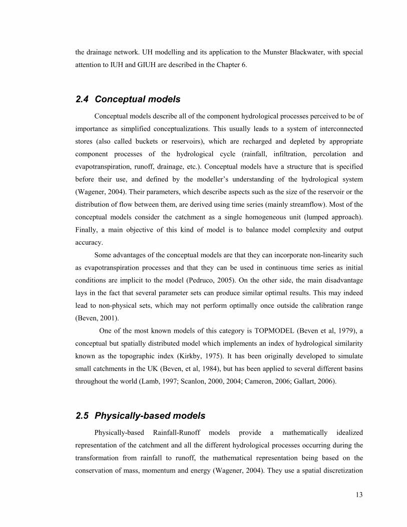
2.4 Conceptual models
Conceptual models describe all of the component hydrological processes perceived to be of
importance as simplified conceptualizations. This usually leads to a system of interconnected
stores (also called buckets or reservoirs), which are recharged and depleted by appropriate
component processes of the hydrological cycle (rainfall, infiltration, percolation and
evapotranspiration, runoff, drainage, etc.). Conceptual models have a structure that is specified
before their use, and defined by the modeller’s understanding of the hydrological system
(Wagener, 2004). Their parameters, which describe aspects such as the size of the reservoir or the
distribution of flow between them, are derived using time series (mainly streamflow). Most of the
conceptual models consider the catchment as a single homogeneous unit (lumped approach).
Finally, a main objective of this kind of model is to balance model complexity and output
accuracy.
Some advantages of the conceptual models are that they can incorporate non-linearity such
as evapotranspiration processes and that they can be used in continuous time series as initial
conditions are implicit to the model (Pedruco, 2005). On the other side, the main disadvantage
lays in the fact that several parameter sets can produce similar optimal results. This may indeed
lead to non-physical sets, which may not perform optimally once outside the calibration range
(Beven, 2001).
One of the most known models of this category is TOPMODEL (Beven et al, 1979), a
conceptual but spatially distributed model which implements an index of hydrological similarity
known as the topographic index (Kirkby, 1975). It has been originally developed to simulate
small catchments in the UK (Beven, et al, 1984), but has been applied to several different basins
throughout the world (Lamb, 1997; Scanlon, 2000, 2004; Cameron, 2006; Gallart, 2006).
2.5 Physically-based models
Physically-based Rainfall-Runoff models provide a mathematically idealized
representation of the catchment and all the different hydrological processes occurring during the
transformation from rainfall to runoff, the mathematical representation being based on the
conservation of mass, momentum and energy (Wagener, 2004). They use a spatial discretization

14
based on grids, hill slopes or some kind of hydrologic response unit. Most of their parameters
have physical significance and are obtained from field measurements. They became practically
usable in the 1980s, as a result of improvements in computer power. Their development was
motivated by a will to obtain some models that could be run without any calibration step, i.e.
which would be applicable to ungauged catchment or to catchment where available data is not
enough to calibrate metric or conceptual models.
Unfortunately, mechanistic models suffer from extreme data demand, scale-related
problems and over parameterization (Beven, 1989) and still require to go through a calibration
phase in order to determine some key parameters (Wagener, 2004). They are then applied in a
way that is similar to lumped conceptual models, without necessarily getting more accurate
results than simpler approaches. Furthermore, the high complexity of physical models generally
requires large amounts of computing time, which make them for example, unsuitable for live
flood forecasting. Finally, some of the physical parameters (especially subsurfaces processes) are
commonly derived in small scale laboratory experiments and are then extrapolated catchment
scale, which often leads to incorrect values and loss of the heterogeneity of the catchment
(Wheater, 2002).
The TIN-based real-time interactive basin simulator (tRIBS) model (Ivanov et al, 2004)
is a fully-distributed, triangulated irregular network (TIN) mechanistic model updated from the
real-time interactive basin simulator (RIBS) (Garrotte, 1993). First developed for its application
to Illinois River at Watts where it showed good results, it was also applied to the Munster
Blackwater catchment (Steinmann, 2004). Really demanding in term of input, tRIBS needs a lot
of input parameters (9 parameters concerning the vegetation properties, e.g. canopy capacity or
optical transmission coefficient; 11 parameters for the soil hydraulic and thermal properties, e.g.
saturated hydraulic conductivity or saturation soil moisture content; 5 parameters for channel and
hillslope routing parameters, e.g. channel roughness coefficient or hillslope velocity coefficient),
an elaborated TIN, soil and land use information, the groundwater spatial distribution, rainfall
input (either radar-rainfall of raingauge data) and some meteorological data inputs (e.g.
atmospheric pressure, relative humidity). Such a complexity leads to complex data collection and
transformation, and to high calculation times. After calibrating and testing the model on 5 floods
between January 2002 and January 2005, it was concluded that even if the results were
promising, the model’s accuracy was lower than the one obtained with the much simpler ANN
metric model (Corcoran, 2004; Leahy, 2006).

15
2.6 Hybrid metric-conceptual models
These types of model are driven by observational data, and are used to investigate
hypothesis regarding the hydrological processes and storages of a system (Wheater et al, 1993). It
uses statistical investigation of the data to determine the structure of the model. The resulting
structure and parameters are then used to investigate the structure of the hydrological system. It is
usual for these models to be run on a continuous basis and incorporating initial conditions directly
into the model (Pedruco, 2005). Model’s inputs (usually rain and potential evapotranspiration) are
linearly combined to produce output (stream discharge). The main drawbacks of this category is
that it took its metric model parent characteristic of being seen as a “black-box” model (Tilford,
2003) and that the assumption of linearity may not be justified for the entire range of flows.
The Rainfall-Runoff Modelling Toolbox (RRMT) (Wagener et al, 2001) provides its user
with different hybrid lumped models and was used to simulate phosphorus transfer in the River
Enborne (UK) (Smith, 2005). Two different hybrid metric-conceptual models were evaluated,
both driven by readily available rainfall, potential evaporation and land use data, in order to
generate daily estimates of flow and in-stream P concentrations.

16
Chapter 3 Catchment description
17
3.1 Ireland
3.1.1 Introduction
Before describing the Blackwater catchment, a brief introduction to Ireland with respect
to hydrology is given. The location, topography, rivers, geology, soils and land uses
characteristics are given in order to highlight different aspects of Irish hydrology. Climatic
impacts, which is a major factor in all hydrology is also described.
3.1.2 Location
Ireland, which is the third biggest island in Europe, is located on the far western end of
the European continent, surrounded by waters of the Atlantic Ocean on its West and the Irish Sea
on its East. The total area of the “Emerald Isle” is 84,000 km2 with 69 000 km2 being the
Republic of Ireland.
3.1.3 Topography
With only a few peaks, Ireland has a relatively low elevation (the majority of the island is
less than 150 meters above sea level). Only 5% of the total area has an elevation between 300 and
600 m a.s.l and only 0.2% at a height of greater than 600 m a.s.l (Rohan, 1975). Most of the
highest peaks are located in the South-West of the country (Mt Carrauntoohil, the highest at
1041m a.s.l) (Rohan, 1975). The topography features a hilly, central lowland surrounded by a
broken border of coastal mountains. The mountain ranges vary greatly in geological structure.
Ireland has often been described as saucer or bowl shaped.
3.1.4 Geology and soils
Ireland is largely composed of palaeozoic and precambrian rocks (Holland, 2001) with
the Precambrian outcrops of schist, gneiss and quartzite mostly in the North West and palaeozoic
sandstone, limestone and shale over on the rest of the country.
The soils of the centre of Ireland are dominated by luvisols being developed from the
underlying Limestone parent material. These soils are porous and well aerated and have a high
moisture capacity (Food and Agriculture Organisation,2001). Intermixed with these luvisol soils
are histosols which are associated with peat bogs having a high organic content and often being
water logged (Food and Agriculture Organisation, 2001).

18
Surrounding this interior are gleysol soils. The cambisols of the east coast are usually
found in alluvial planes and are freely draining with excellent agricultural properties. The
older podzolic soils are typically found in conjunction with the precambrian and older
palaeozoic rocks. These aged soils are usually of a sandy composition with the upper
horizons being leached due to heavy rainfall. A common occurrence in this type of soil is
mineral precipitation at the bottom of the A horizon where an impermeable crust forms
known as an iron pan. These soils are not known for their water holding capacity nor their
agricultural properties (Food and Agriculture Organisation, 2001).
Figure 3.1 Geology of Ireland (Geological Survey of Ireland)

19
3.1.5 Climate
The dominant influence on Ireland's climate is the Atlantic Ocean. Consequently, Ireland
does not suffer from the extremes of temperature experienced by many other countries at similar
latitude. The other important factor impacting on Ireland’s climate is the westerly atmospheric
circulation of the mid latitudes (Rohan, 1975; Hargy, 1997; Keane & Sheridan, 2004). This
association gives the Irish climate a distinct maritime character which is moderated by the
influence of Gulf Stream.
The average annual temperature of Ireland is about 9 °C. In the middle and east of the
country temperatures tend to be somewhat more extreme than in other parts of the country. For
example, summer mean daily maximum is about 19 °C and winter mean daily minimum is about
2.5 °C in these areas.
Most of the eastern half of the country has between 750 and 1000 mms of annual rainfall.
Rainfall in the west generally averages between 1000 and 1250 mm. In many mountainous
districts, it exceeds 2000mm per year. The wettest months, almost everywhere are December and
January. Hail and snow contribute relatively little to the precipitation measured. During late
summer or early spring depression or anticyclonic conditions may dominate bringing wide spread
rain. This is generally replaced by westerlies through October and November which are relatively
warm and lead to frontal rain (Rohan, 1975). Typically rainfall does not occur in heavy showers
rather as drizzle or rain. Irish rainfall tends to be low intensity over long periods (Rohan, 1975) or
archetypal frontal rainfall which is dominated by the west to east flow of air across Ireland.
Figure 3.2 Mean Annual Rainfall over Ireland (Met Éireann)

20
Figure 3.2 shows the long term mean annual rainfall over the country. A gradient of
precipitation can be seen from West to East, with some higher amounts associated with the high
topography.
3.2 Blackwater catchment
3.2.1 Location
The Munster Blackwater catchment is located in the southwest of Ireland (see figure 3.3).
The catchment is primarily within North West County Cork, Mid Cork and East Cork. The total
area of the catchment is 3324km2 which is almost 4% of the total land area of Ireland (Doheny, J.
1997). The Munster Blackwater catchment drains most of the Northern Division of County Cork
and a large part of east County Waterford.
Figure 3.3 Munster Blackwater catchment location is shown shaded
(Office of Public Work)

21
3.2.2 Topography and river path
The Munster Blackwater catchment is a broad valley surrounded by mountains on its
North (Mullaghareirk Mountains, Seefin Mountains, Galty Mountains and Knockmealdown
Mountains) and its South (Caherbarnagh Moutains, Derrynasaggart Mountains and the
Boggeragh Mountains). The highest point of the catchment is located in the Galty Mountains at
an altitude of 892m a.s.l, while the lowest part of the catchment is at sea level (Youghal). The full
length of the Blackwater from its rising point near Ballydesmond to the sea at Youghal is 134 km.
Figure 3.4 Munster Blackwater catchment topography
The river rises in the foothills of the Mullaghareirk Mountains at Knockanefune (near
Ballydesmond) in County Kerry. The river flows due south to Rathmore along the Cork and
Kerry border. At Rathmore the river turns and flows due east passing near Millstreet and Kanturk
and then through Mallow and Fermoy into County Waterford. At Cappoquin the river turns to
flow due south and enters the sea at Youghal. There are 29 tributaries running into the Blackwater
(Hydrological Data, EPA) the main ones being the Bride, close to Cappoquin, the Awbeg,
between Fermoy and Mallow, the Allow, which is close to Kanturk, and the Owentaraglin which
is close to Millstreet. It is tidal for a distance of approximately 20km upstream to Cappoquin.

22
Figure 3.5 Munster Blackwater river network
3.2.3 Soils and geology
3.2.3.1 Soils
An important soil database is being built by the Environmental Protection Agency (EPA)
which is currently undertaking a Soil Survey for Ireland. Most of the catchment is covered by the
survey except for a small area in the north (see figure 3.6). Soils are classified according to the
Irish Forest Soils (IFS) classification which at level 1 is: deep well drained minerals, shallow well
drained minerals, deep poorly drained minerals, poorly drained minerals with peaty topsoils,
alluvium, peats and miscellaneous.
As can be seen on figure 3.6, most of the Blackwater catchment is covered with deep well
drained minerals. Shallow well drained minerals represent the second proportion and appear in
patches all over the catchment. Poorly drained mineral soils are concentrated in the north-eastern
part of the catchment and the greatest proportions of peats can be found in the western end. As
alluviums cover the main river beds, its location identifies the floodplains.

23
Figure 3.6 Munster Blackwater catchment soil types
The EPA has also funded a Subsoil Survey which, like the Soil Survey, covers almost all
the catchment (see figure 3.7). Most of the valley is covered with materials originated from tills
(TDSs, TLs and TNSSs). Peats can also be found on the western end and bedrock is found at the
surface (Rck) as patches all over the catchment.
Tills are diamicton (nonlithified, nonsorted or poorly sorted sediments that contain a wide
range of particle sizes) deposited by or from glacier ice. They correspond to the well drained and
poorly drained mineral soils. The association of soils and subsoils allows reference to the general
soil map classification and thus give more details about the nature of the soil. Indeed acidic well
drained minerals from tills can be associated, in that area with Brown Podzolics which are
gravelly loams. In the same way acidic poorly drained minerals from tills mostly refer to Gleys
which are clay loams, and acidic shallow well drained minerals to Lithosols which are sandy
loans.
Peat is a post-glacial deposit, consisting mostly of vegetation which has only partially
decomposed. Alluvium is a post-glacial deposit and may consist of gravel, sand, silt or clay in a
variety of mixes and usually consists of a fairly high percentage of organic carbon (10%-30%).
Rocks close to the surface are often associated with shallow well drained areas.

24
Figure 3.7 Munster Blackwater catchment sub-soils types
3.2.3.2 Geology
There are two main rock types in the Munster Blackwater catchment: Devonian
Sandstone is the principal rock type to the South and Dinantian Limestone is the dominant rock
type north of the river (Geological Survey of Ireland, 2004).
.
Figure 3.8 Munster Blackwater catchment bed rock geology (Corcoran, 2004)

25
3.2.4 Land uses
Land use information and spatial distribution is available trough the CORINE (Co-
Ordination of Information on the Environment) Land Cover database elaborated by the EPA. The
survey covers the whole catchment and classifies the different land uses using three different
levels. Figure 3.9 shows a graphical repartition of the different land uses, according to the 1st
level of CORINE nomenclature.
Figure 3.9 Munster Blackwater catchment land uses
Agriculture is dominant with more than 90% of it being grassland. Forest and semi-
natural areas come second with a much lower proportion. The artificial surface over the
catchment represents a really small amount of the total area, which mainly reflects the low
urbanization level of the catchment. The main artificial surfaces area (orange colour on figure
2.4) being the town areas of Kanturk, Millstreet, Mallow, Fermoy, Mitchelston and Youghal.
3.2.5 Climate
Precipitation over the catchment is the most important climatic factor for hydrological
response. Precipitation can be considered as being the rainfall only considering the really low
occurrence of snow and hail. The catchment has a 1200 mm annual average rainfall and a 300-
400 mm evapotranspiration (Corcoran, 2004). The rainfall occurs during the whole year with

26
amounts from October to March. Evapotranspiration losses are considered significant only during
the summer months (May to September). Precipitation amounts are higher on the western edge of
the catchment and around the highest hills and peaks. The rainfall regime is characterized by
long duration events of low hourly intensity. Short duration events of high intensity are more
seldom and mostly occur in summer. A more precise study of the catchment rainfall is reported
Chapter 4.
Considering the catchment latitude, the daily air temperatures over the course of the year
have a small range of variation, mainly because of the influence of the warn Gulf Stream.
Temperatures go from a maximum of ~20ºC to a minimum of ~0ºC, with an average of 15ºC in
summer and 5ºC in winter (Jaksic, 2004).
The UCC Hydromet research group runs a meteorological station in Dounoughmore, 5km
south of the catchment. Data recorded there are considered to be representative of the
meterological conditions within the studied catchment. Figure 3.10 shows two annual wind roses
recorded in Dounoughmore. It can be seen that the prevailing wind direction is from the
southwest.
Figure 3.10 Wind roses (a) for 2002 and (b) for 2003 (Jaksic, 2003)
The general pattern of river flow in the Munster Blackwater is a temperature oceanic
river regime (Corcoran, 2004).
3.2.6 Subcatchments
Some particular subcatchments will be considered in the following chapters. Those have
been chosen considering the availability and the quality of their data. Three main Subcatchments
were considered, Duarrigle, Dromcummer and Killavullen. Table 2.6 gives the area, the river
length to the outlet and the S-1085 slope.

27
Table 3-1 Nested sub-catchments
Catchment Area (km2) Length (km) Slope – S1085
Duarrigle 245 21 3.9
Dromcummer 861 39 2.7
Killavullen 1292 68 2
Figure 3.11 Duarrigle, Dromcummer and Killavulen nested sub-catchments

28
Chapter 4 Rainfall Analysis

29
4.1 Introduction
Precipitation data is the most important hydrologic parameter in the hydrological study of
the Blackwater. Obtaining reliable data over time and space was an essential step before
modelling the rainfall-runoff. Irish rainfall is being recorded at many places by the
Meteorological Office. The time step of the records is either hourly or daily. A lot of effort was
put in obtaining as much rainfall data as possible covering the catchment. In the following
chapter, the different sources of rainfall data are discussed and trends of rainfall over the
catchment are analysed.
4.2 Meteorological Office data
The Irish Meteorological Office monitoring network has 14 synoptic stations around
Ireland providing hourly reading of temperature, precipitation, wind speed and direction,
sunshine, cloud cover, pressure, humidity, soil and grass temperature, with evapotranspiration and
solar radiation being measured at some of these stations (Sweeney et al., 2002). Daily
temperature and precipitation are measured at over 100 climatological stations and sunshine, soil
and earth temperatures being recorded at some (Keane, 1986). Additionally there are a further
1850 stations which measure daily rainfall (Sweeney et al., 2002). All are data collected and
quality controlled by Met Éireann. Unfortunately, none of the 14 synoptic stations is located in
the Blackwater catchment. Thus, daily rainfall data was provided by the Meteorological Office
with some hourly data from their sites with non digitised paper autographic records.
4.2.1 Automatic raingauges
Some of Met Éireann stations are still operating with automatic gauges. An automatic
driven pencil directly plots the rainfall intensity on a 24-hours chart that has to be changed every
day. When well operated, this kind of raingauge can provide a good 1-hour step dataset.
Unfortunately, changing the chart every day represents a heavy constraint that often causes the
rainfall of different days to be recorded on the same chart. Those charts are generally not digitised
by Met Éireann but retained for further analysis if required. Figure 4.1 gives an example of a 24-
hours recording chart.
Some of the data requested from the Met Service for Millstreet, Freemount and Mallow
(for the period 1988 to 2000) were only available in hard copies stored in the Meteorological
Office Headquarter in Dublin. Digitising of those were expensive as it was necessary to go to

30
Dublin and spend a lot of time translating the hard copy charts into Excel files that were then
usable.
Nowadays, at a time when automatic digital recording raingauges are easy to use and are
affordable, such a method of recording and storing the information is obsolete. Furthermore, as
the data is not digitised nor used afterwards, it seems that putting efforts in this data collection
scheme is expensive on time and money. Replacing these gauges by automatic gauges with
integrated digital data loggers would provide a good quality rainfall dataset, and would require
less work as this kind of modern loggers can be downloaded every few months and the obtained
data directly available as usable digital tables.
Each time the 24-hours chart is not changed, rainfall for consecutive days are
superimposed which makes it difficult to extract the data corresponding to each day. When
confronted with this situation, the different curves were compared to those corresponding to the
same days in a station nearby, that allowed us to recognise the rainfall variation over time and
then choose the appropriate values. Figure 4.1 shows an example of two superposed daily plots.
Figure 4.1 Example of an automatic raingauge chart (Met Service)

31
4.2.2 Daily rainfall
The Meteorological Office has built a large daily rainfall data set over Ireland. Figure 4.2
shows all the available raingauges within the Blackwater catchment. All the still operating
stations, their coordinates and their opening dates are listed in table 4.2.
Figure 4.2 Met Service daily raingauges network
Data was requested for all the still operating stations. Mr Niall Brooks (Climatological
Division, Met Éireann) forwarded data to us as tables indicating the date, the rainfall depth and an
indicator code. This indicator code identifies the quality of the data and their description is given
in Table 4.1.
Table 4-1 Raingauge data indicator code description
Code Description
0 Satisfactory
1 Estimated
2 Cumulative, no reading
3 Estimated cumulative total
4 Trace
5 Estimated trace
6 Cumulative trace
7 Estimated cumulative trace
8 Not available
9 Cumulative total

32
As suggested by the indicator code table, all stations show gaps in their data (due to
equipment failure or operator absence) and periods where rainfall depth is measured over a
cumulative period of a few days. These cumulative values are not considered as a problem when
dealing with weekly, monthly or yearly data, but have to be avoided when using daily data.
Table 4-2 Still operating daily raingauges in the Blackwater catchment
ID Station Number
Name X Y Open
1 706 MALLOW (HAZELWOOD) 155596 104416 1941
2 1106 CAPPOQUIN (MT.MELLERAY) 209549 104071 1944
3 1406 KANTURK (VOC.SCH.) 138481 103207 1944
4 3606 FERMOY (MOORE PARK) 181991 101313 1961
5 3706 RATHLUIRC (FOR.STN.) 157331 118466 1962
6 4006 KNOCKANORE 207577 89076 1964
7 4106 YOUGHAL (GLENDINE W.W.) 206440 83820 1982
8 5206 NEWMARKET BALLINATONA P.H. 128406 112246 1982
9 5306 MOUNT RUSSELL 161321 119793 1984
10 3806 YOUGHAL (ST.RAPHAEL'S HOSP.) 210173 77490 1963
11 5506 BALLINAMULT (DOON) 217253 106719 1984
12 6206 LOMBARDSTOWN (DROMPEACH) 146327 94120 1985
13 6306 BANTEER LYRE 141566 92443 1985
14 5406 GALTEE MOUNTAINS SKEHEENARINKY 188724 119407 1984
15 6406 TALLOW KILMORE 201288 91265 1986
16 6506 MILLSTREET SEWAGE WORKS 127507 90927 1986
17 6606 MALLOW (SEWAGE TREATMENT) 157592 97937 1988
18 6906 MILLSTREET (COOMLOGANE) 126039 90856 1991
19 7006 BARTLEMY 181903 87558 1992
20 7306 NEWMARKET (NEW STREET) 131603 107471 1993
21 7406 MALLOW (SPA HOUSE) 156572 98688 1996
22 7506 BANTEER (GLENSOUTH) 142539 92586 1997
23 7706 TALLOWBRIDGE 199860 94882 2000
24 7806 MITCHELSTOWMN (CORK STREET) 181768 112751 2000
25 7906 BALLYHOOLY (CASTLEBLAGH) 171990 97526 2001
26 8006 GLENCAIRN (TOURTANE HOUSE) 203341 96676 2001
27 8106 CAPPOQUIN (STATION HOUSE) 210623 99159 2002
28 8206 MITCHELSTOWN (GLENATLUCKEY) 183066 109655 2001
29 8306 SHANBALLYMORE 167205 107509 2002
30 8406 CONNA (CASTLEVIEW) 195672 94482 2003
31 8506 LISMORE 204862 97975 2003
32 5706 CASTLEMAGNER 142535 103746 1985
33 5806 FREEMOUNT PUMPING STATION 139372 113862 1984
34 906 RATHMORE G.S. 117026 93163 1941

33
4.3 The Office of Public Works data
4.3.1 Project
The Office of Pubic Works is currently undertaking a Flood Studies Update (FSU) over
several Irish catchments, one of them being the Munster Blackwater River. UCC Flood Studies
Group has been hired to provide the preliminaries of the project, which include different tasks:
management of a raingauges network, data collection, data analysis and flood event analysis.
4.3.2 Recording network description
32 raingauges were installed in order to determine the spatial variation of rainfall over the
catchment. These were installed between August and October 2005 and the data set is in service
since November 2005.
Figure 4.3 OPW 32 raingauges network
As can be seen on the figure 4.3, all the catchment, except from a small area in the south-
east (around the Youghal estuary) is covered with this dense network. The longest distance
between one raingauge and its furthest neighbour being 19 km (between BottleHill and
Bartlemy).

34
The 32 units were installed in different locations owned by Cork County Council (mostly
wastewater treatment plants, reservoirs, water intake plants and landfills) in order to facilitate
their access and improve their security.
Table 4-3 OPW raingauges network in the Blackwater catchment
Name Four letters name
Irish National Grid
Elevation (meters a.s.l.)
Bottle Hill - Pump House Bott W610884 210
Bweeng - Pump House Bwee W493878 220
Lyre - Reservoir Lyre W405919 280
Kilcorney - Reservoir Kilc W337903 220
Millstreet - Reservoir Mill W260893 200
Buttervant - Pump House Butt R533084 105
Ballyhoura Way - Water intake works Chur R528143 95
Freemount - Waste water treatment plant Free R394139 140
Meelin - Water treatment plant Balt R290118 200
Newmarket - Reservoir Newm R316070 180
Ballydesmond - Pump house Bald R150038 215
Knocknagree - Old pump house Knoc W185978 170
Duhallow Way - Reservoir Ratm W176885 290
Kanturk - Waste water treatment plant Kant R384017 80
Mallow - Pump house Mall W541957 60
Kishkeam - Waste water treatment Kish R207038 200
Rathcoole - Waste water treatment plant Ratc W334941 100
Pallas - Old pump house Lomb W455981 105
Doneraile - Pumphouse Done R586075 80
Kilbrin - Resevoir Kilb R429071 190
Two Pot House - Resevoir Twop R571025 120
Ballygugroe - Landfill Balg R662145 220
Kildorrey - Sewage Works Kild R717106 75
Mitchelstown - Water Treatment Plant Mitc R809133 90
Castlecooke - Pumphouse Kilw R877046 110
Bartlemy - Pumphouse Bart W817885 130
Fermoy - Pumphouse Ferm W776982 40
Coole - Pumphouse Cool W868950 80
Tallow - Resovoir/Pumphouse Tall W008922 80
Lismore - Resevoir/Pumphouse Lism S061014 175
Cappoquin - Cappoquin Capp X133977 18
Killavullen - Water Treatment Plant Kill W648994 50
35
4.3.3 Instrumentation and site management
Each site is provided with a raingauge, linked to an external data logger which is stored
in a plastic security box near the gauge.
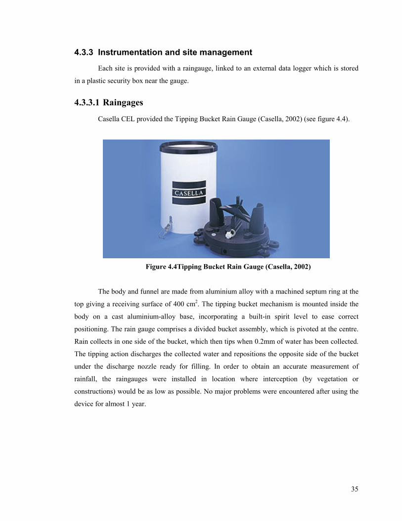
4.3.3.1 Raingages
Casella CEL provided the Tipping Bucket Rain Gauge (Casella, 2002) (see figure 4.4).
Figure 4.4Tipping Bucket Rain Gauge (Casella, 2002)
The body and funnel are made from aluminium alloy with a machined septum ring at the
top giving a receiving surface of 400 cm2. The tipping bucket mechanism is mounted inside the
body on a cast aluminium-alloy base, incorporating a built-in spirit level to ease correct
positioning. The rain gauge comprises a divided bucket assembly, which is pivoted at the centre.
Rain collects in one side of the bucket, which then tips when 0.2mm of water has been collected.
The tipping action discharges the collected water and repositions the opposite side of the bucket
under the discharge nozzle ready for filling. In order to obtain an accurate measurement of
rainfall, the raingauges were installed in location where interception (by vegetation or
constructions) would be as low as possible. No major problems were encountered after using the
device for almost 1 year.

36
Figure 4.5 To avoid interception, the gauge is installed on the roof of a reservoir in
Knocknagree
4.3.3.2 Data loggers
Casella was also selected to provide the logging equipment. Casella Sensus Logger
(Casella, 2002) (see figure 4.6) is an external multi channel data acquisition module and can thus
be used for many measurements devices in the same time (rainfall, temperature, wind speed, wind
direction, etc.). The OPW decided to use this complex device, obviously capable of a lot more
than raingauge logging with the idea of implementing other measurement devices in the future.
Figure 4.6 Sensus Logger (Casella, 2002)

37
Logging could originally be set at different time interval (from 1 minute to one day) and
information could be stored in the internal memory for a long period of time. The Sensus was
originally powered by a 12v d.c. 7Ah Lead Acid battery that was supposed to have a 2 months
life time if logging every 5 minutes. Data can be downloaded via a RS232 port to laptop or
palmtop devices, and directly saved as friendly format files. Communications between the user
and the logger are made through the Online Pro Software (Casella CEL, 2002) which allows
uploading and downloading settings to and from the logger, to download the recorded data and to
display the information. The Sensus is kept in a hermetic plastic shelter (30 x 30 x 18 cm) within
a meter or two of the gauge (see figure 4.7).
Figure 4.7 The raingauge and its data logger in Bweeng
38
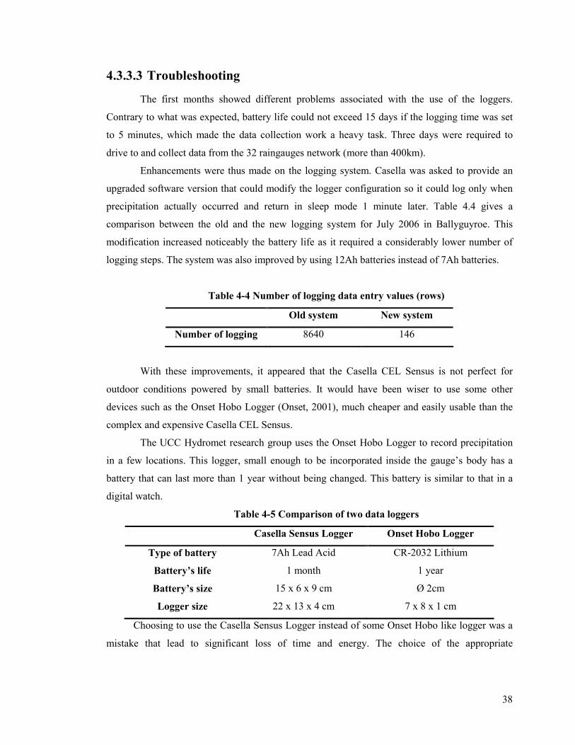
4.3.3.3 Troubleshooting
The first months showed different problems associated with the use of the loggers.
Contrary to what was expected, battery life could not exceed 15 days if the logging time was set
to 5 minutes, which made the data collection work a heavy task. Three days were required to
drive to and collect data from the 32 raingauges network (more than 400km).
Enhancements were thus made on the logging system. Casella was asked to provide an
upgraded software version that could modify the logger configuration so it could log only when
precipitation actually occurred and return in sleep mode 1 minute later. Table 4.4 gives a
comparison between the old and the new logging system for July 2006 in Ballyguyroe. This
modification increased noticeably the battery life as it required a considerably lower number of
logging steps. The system was also improved by using 12Ah batteries instead of 7Ah batteries.
Table 4-4 Number of logging data entry values (rows)
Old system New system
Number of logging 8640 146
With these improvements, it appeared that the Casella CEL Sensus is not perfect for
outdoor conditions powered by small batteries. It would have been wiser to use some other
devices such as the Onset Hobo Logger (Onset, 2001), much cheaper and easily usable than the
complex and expensive Casella CEL Sensus.
The UCC Hydromet research group uses the Onset Hobo Logger to record precipitation
in a few locations. This logger, small enough to be incorporated inside the gauge’s body has a
battery that can last more than 1 year without being changed. This battery is similar to that in a
digital watch.
Table 4-5 Comparison of two data loggers
Casella Sensus Logger Onset Hobo Logger
Type of battery 7Ah Lead Acid CR-2032 Lithium
Battery’s life 1 month 1 year
Battery’s size 15 x 6 x 9 cm Ø 2cm
Logger size 22 x 13 x 4 cm 7 x 8 x 1 cm
Choosing to use the Casella Sensus Logger instead of some Onset Hobo like logger was a
mistake that lead to significant loss of time and energy. The choice of the appropriate

39
instrumentations is a really important task when installing a scientific survey scheme and should
always be advised by actual scientists working in the field more than by traders.
4.4 UCC Hydromet data
The UCC Hydromet research group also ran 5 raingauges in the Mallow subcatchment for
the full year 2005. Rainfall was recorded on an hour basis using the previously presented Onset
Hobo Logger. The five recording locations are listed in table 4.6.
Table 4-6 Location of Ucc Hydromet gauges
Name X Y Irish National Grid
Banteer 141500 92500 W415250
Millstreet 127400 90600 W274060
Ballydesmond 114900 104000 R149040
Newmarket 128300 112300 R283123
Castlemagner 142500 103800 R425038
4.5 Raingauges contributing areas
When a basin has more than one raingauge in the area considered, these raingauges
inevitably record different amounts of precipitations whether it is for a single rainstorm or over a
specified period of time. In this chapter, contributing areas of each raingauges are defined using
the Thiessen polygon associated with each station. The Thiessen polygon of a gauge is the region
in which any point at random is closer to this particular gauge than to any other gauge in the
recording network. The precipitation is assumed to be constant and equal to the gage value
throughout the whole region. It should be noted that
Here, a gauge represents a sub area Ai which denotes the area of influence of each gauge
which is obtained by constructing polygons determined by drawing perpendicular bisectors to
lines connecting the gauges. The bisectors are the boundaries of the effective area for each gauge,
each enclosed are can be measured using GIS tools. The spatial average is calculated by
weighting the individual stations with their respective area given by:
∑=
=n
i
iiPAA
P1
1 (4.1)

40
where n is the number of raingauges in the area, and Ai is the surface area of the catchment, that is
the sum of the sub areas, or ∑=
=n
i
iAA1
.
It should be noted that even if the Thiessen polygons method is the most widely used, it
does not take into account the elevation factor and that the denser the recording network is, the
more reliable the Thiessen method will be.
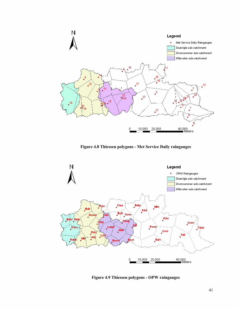
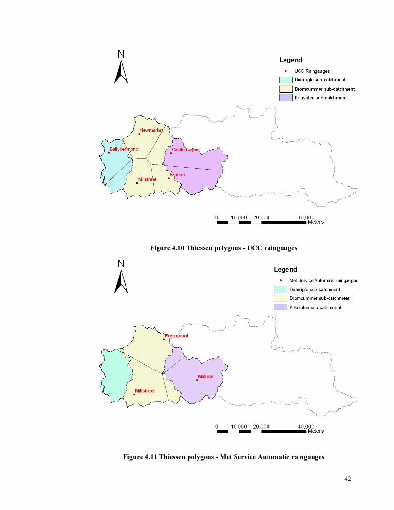
In the following chapters of this thesis, rainfall-runoff modelling is applied to 3 sub-
catchments within the Blackwater catchment (Duarrigle, Dromcummer and Killavulen). Thiessen
polygons were therefore constructed regarding to these areas (see figures 4.8 to 4.11). The
construction has to be made for all the different recording networks used for the corresponding
dates (see table 4.7). Average rainfall data over each sub-catchment can be determined as a
weighted average (regarding to the surface areas) of its Thiessen polygons.
Table 4-7 Recording step and period of availability for the different recording network
Data source Recording step Period of availability
Met Service daily gauges 1 day 1941 to now (depending on the gauge)
Met Service Automatic Gauges 1 hour 1988 to 2004
UCC Hydromet 5 minutes 2005
OPW 5 minutes November 2005 to now
41
Figure 4.8 Thiessen polygons - Met Service Daily raingauges
Figure 4.9 Thiessen polygons - OPW raingauges
42
Figure 4.10 Thiessen polygons - UCC raingauges
Figure 4.11 Thiessen polygons - Met Service Automatic raingauges

43
4.6 Analysis
4.6.1 Comparison between the different sources
The daily Met Éireann data and the 5-minutes step OPW data cover a mutual period of
record (from the 1st of November 2005 to the 1st of August 2006). Data was compared in
locations where both Met Éireann and OPW gauges could be found. In order to be representative
of the spatial variation, three locations were particularly analysed: Millstreet in the West, Mallow
in the catchment centre and Tallow in the East.
Table 4-8 Comparison between Met Eirean daily raingauges and new OPW gauges
Millstreet Mallow Tallow
Met Éireann (mms) 661 419 416
OPW (mms) 734 486 485
OPW/Met 1.11 1.16 1.16
For each of the three locations, a strong linear relationship is observed between the two
sources of data (see figure 4.13), but the depths recorded by the Met Éireann appear to be lower,
with an approximate linear coefficient of 15% (this underestimation was noticed in the whole
recording network). A one day scale comparison tells more about the difference in depths. Figure
4.12 gives an example of a two weeks observation period in Mallow.
Mallow, 11th to 28th February 2006
0.0
2.0
4.0
6.0
8.0
10.0
12.0
1 2 3 4 5 6 7 8 9 10 11 12 13 14 15 16 17 18
Days
Rain (mm)
Met Eireann
OPW
Figure 4.12 One day scale comparison between Met Éireann and OPW data

44
Figure 4.13 Comparison between Met Éireann raingauges and new OPW gauges

45
At this scale, the constant underestimating is not observed. We can see that the OPW
depths are sometime lower than the ones observed by Met Éireann. This apparent absence of
linear relationship between the two dataset may be explained by the data collection operating
mode. Most of Met Éireann gauges are manually checked on a daily basis. As data are given for
9am to 9am day, late reading in the morning will imply an erroneous value, especially on a day
when it is actually raining around the reading time. Furthermore, every fault in reading the gauge
will imply a 2 days cumulative value for the next day. This issue is reflected in the Data Indicator
Description given with each value by Met Éireann (see table 4.1).
Considering the high correlation observed for the 6 months cumulative rain comparison,
Met Éireann data was considered accurate enough to be used. Nevertheless, the OPW data, with
its very precise 5 minutes-step dataset, was preferred as soon as available. Considering this point,
all the rainfall studies carried in the following chapter were made using OPW data coming from
the 32 raingauges network of the Munster Blackwater Catchment, for the 9 months of data
available at the time of the writing (November 2005 to July 2006).
4.6.2 9 months data
4.6.2.1 Daily and monthly analysis
The wettest day in the 9 months was recorded on the 12th January 2006 (Julian day 377),
when 41.4 mms were recorded in Rathmore (see figure 4.14). Most of the stations (14) had their
wettest day on the 21st May 2006 (Julian day 506), when a maximum of 36.4 mms was recorded
in Kishkeam and a minimum of 19.8 mms in Kildorrey.
Figure 4.14 Daily Rainfall in Rathmore (9 months data)

46
Figure 4.15Cumulative rainfall for the 32 stations, November 2005 to July 2006.
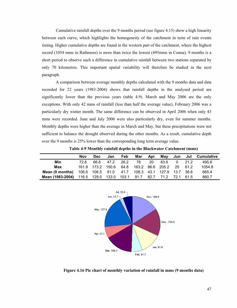
47
Cumulative rainfall depths over the 9 months period (see figure 4.15) show a high linearity
between each curve, which highlights the homogeneity of the catchment in term of rain events
timing. Higher cumulative depths are found in the western part of the catchment, where the highest
record (1054 mms in Rathmore) is more than twice the lowest (495mms in Conna). 9 months is a
short period to observe such a difference in cumulative rainfall between two stations separated by
only 70 kilometres. This important spatial variability will therefore be studied in the next
paragraph.
A comparison between average monthly depths calculated with the 9 months data and data
recorded for 22 years (1983-2004) shows that rainfall depths in the analysed period are
significantly lower than the previous years (table 4.9). March and May 2006 are the only
exceptions. With only 42 mms of rainfall (less than half the average value), February 2006 was a
particularly dry winter month. The same difference can be observed in April 2006 when only 43
mms were recorded. June and July 2006 were also particularly dry, even for summer months.
Monthly depths were higher than the average in March and May, but these precipitations were not
sufficient to balance the drought observed during the other months. As a result, cumulative depth
over the 9 months is 25% lower than the corresponding long term average value.
Table 4-9 Monthly rainfall depths in the Blackwater Catchment (mms)
Nov Dec Jan Feb Mar Apr May Jun Jul Cumulative
Min 72.6 66.6 47.2 26.2 76 20 83.6 0 21.2 495.6
Max 161.8 173.2 150.6 64.8 163.2 86.6 205.2 25 61.2 1054.8
Mean (9 months) 106.6 106.5 81.0 41.7 108.3 43.1 127.9 13.7 36.6 665.4
Mean (1983-2004) 116.5 129.0 133.0 103.1 91.7 82.7 71.2 72.1 61.5 860.7
Figure 4.16 Pie chart of monthly variation of rainfall in mms (9 months data)

48
As can be seen in figure 4.17, the range of monthly records between the different stations
depends with the period of the year. The three wettest months (December, March and May) have
the more spread ranges.
Figure 4.17 Monthly box plots (9 months data)
4.6.2.2 Drought assessment
A long flat part from the end of May to end of the records (about 80 days, i.e.
approximately 30% of the data length) can be observed in each of the 32 raingauges (see figure
4.15). Such a long period without significant rain events is not common in Ireland and does not
reflect the monthly average values usually recorder in this catchment. In order to judge the
importance of this dry period, daily rainfall records were compared with data from the summer
1976, when the more important ever recorded drought in Ireland was observed (McCartaigh,
1996).
Periods of little or no rain are described using the terms introduced by Met Éireann, that
are more useful than the World Meteorological Organisation (WMO) definition, and more
quantifiable for the conditions pertaining in Ireland. An absolute drought is a period of 15 or more
consecutive days, on none of which 0.2 mm or more of rain fell. A partial drought is a period of at
least 29 consecutive days, the mean daily rainfall of which does not exceed 0.2 mm. Finally, a dry
spell is a period of 15 or more consecutive days, on none of which 1.0 mm or more of rain fell.
Table 4.10 gives the number of days that meet the requirements for absolute droughts,
partial droughts and dry spells.

49
Table 4-10 Number of days fulfilling the requirements for the different drought
indicators
Station Absolute drought Requirements
(needs to be >15)
Partial drought Requirements
(needs to be >29)
Dry spell Requirements
(needs to be >15)
Bottle Hill 22 31 22
Bweeng 13 14 13
Lyre 13 14 14
Kilcorney 13 14 14
Millstreet 13 14 14
Buttevant 13 24 14
Churchtown 11 20 22
Freemount 14 23 22
Balinatona 14 23 14
Newmarket 14 22 14
Ballydesmond 13 14 14
Knocknagree 13 24 22
Rathmore 14 14 14
Kanturk 13 22 14
Mallow 13 14 14
Kishkeam 14 22 15
Rathcoole 13 19 14
Lombardstown 13 22 16
Doneraile 13 22 14
Kilbirn 13 22 13
Two Pot House 13 22 13
Ballyguyroe 12 20 23
Kildorrey 13 22 22
Mitchelston 13 22 14
Kilworth 13 24 22
Bartlemy 13 14 13
Fermoy 13 14 14
Cool 14 28 14
Tallow 13 28 14
Lismore 14 24 14
Cappoquin 13 28 24
Killavulen 13 14 14
Among the 32 stations, only one absolute drought was recorded, in Bottle Hill, where no
rainfall was recorded for a total period of 21 days (from 27th May to 17th June 2006). Most of the
stations located in the Western part of the catchment saw at least 12 days (from 27th May to 10th
June 2006) without any rainfall, while the total absence of rainfall lasted 13 days (from 27th May to
11th June 2006) in most of the Eastern locations. It should be noted that such a long period without
any rainfall at all was not observed in 1976, where no absolute drought occurred (MacCarthaigh,
1996).

50
The partial drought analysis also showed that Bottle Hill was the only station to meet the
requirements, with a 31-days period from the 27th May to the 26th June. Three other Eastern
stations (Fermoy, Coole and Lismore) recorded 28 consecutive days the mean daily rainfall of
which did not exceed 0.2 mm, and where therefore just below the threshold of 29 days. In 1976, a
33 days long period of partial drought was observed in Fermoy Moorepark. The longest dry spell
was observed in Cappoquin from the 27th May to the 20th June 2006 (24 days). Dry spells were
also observed in 8 other stations from the 27th May (Bottle Hill, Churchtown, Freemount,
Knocknagree, Lombardstown, Ballyguyroe, Kildorrey and Kilworth). It should also be noted that
dry spells, unlike absolute and partial droughts, occurred at other different time in the year (after
the 13th November 2005, the 21st January and the 28th May) for a majority of the 32 recording
stations. In 1976, the longest dry spell lasted only 22 days in Fermoy Moorepark. A small amount
of rainfall, falling at the end of a drought, may break the formal definition of an absolute/partial
drought but may not be sufficient to cause surface runoff or may cause a small amount of surface
runoff. In the latter case, the river levels will return very quickly to the pattern which pertained
prior to the rainfall because the groundwater component has not increased. For this reason,
MacCarthaigh defines a term called “periods of insignificant rainfall” which have regard to the
runoff effects of small rainfall amounts in drought periods, and is used to asses the severity of
droughts in conjunction with river flow records. A period of insignificant rainfall (PIR) starts with
a period of no rainfall and ends when the corresponding river flow stops to decrease. Unlike the
absolute drought, partial drought and dry spell, the definition of a PIR is subjective. The length of
the period is decided from the observation of both rainfall and river flow data.
Figure 4.18 shows daily river flows in 1976 and 2006, from the 1st of January to the 30th of
September. It should be noted that due to missing data in Killavulen river station, the 2006 plot
was taken from Duarrigle data. The only observed factor being the hydrograph shape (in order to
know if the flow is following a recession), flow values are neglected, and the fact that general
trend was the same in both Killavulen and Duarrigle allow us to compare the two plots. As shown
in figure X, a long period of flow recession ant therefore a PIR is observed from the 27th May to
the 1st September 2006, i.e. 95 days. According to MacCarthaigh, the longest PIR ever recorded in
the Blackwater was 66 days (15th July to 18th September 1976). Another PIR was observed from
the 17th May to 5th July 1976.
Taking into account only the longest absolute droughts, partial droughts, dry spells and
PIRs would lead to consider the 2006 drought as being more important than the one observed in
1976. Figure 4.18 is nonetheless showing longest periods of flow recessions in 1976 than in 2006,
physical sign of a dryer period.

51
Figure 4.18 Comparison of river flows, 1976 and 2006

52
4.6.3 Spatial variation
Rainfall depths recording at different points in the catchment show a high spatial
variability. Coupling the precise OPW dataset and the long term Met Éireann daily dataset
provides a good understanding of this variation.
An effective way to visualize the rainfall spatial variation is to examine rainfall contours,
which display lines where rainfall amounts are constant. Such visualization highlights the different
peaks, slopes and low intensity areas. As can be seen on figure 4.19, rainfall contours constructed
from the 9 months cumulative rainfall show that the wettest areas are located on the western edge
of the catchment and the rainfall seems to decrease with the longitude (from West to East), with a
reduction in the increase at the eastern edge. This tendency is also noticeable in figures 4.15 (9
months cumulative rainfall) where cumulative depths appear to be greater in the West. As outlined
in chapter 2, the main wind direction is from South West. Winds that blow over the catchment
come from the Atlantic Ocean where it is loaded with moisture. Once reaching the boundary
between ocean and land, the moisture is lifted above and condensed in clouds that would cause
precipitation when going over the land. This meteorological phenomenon explains the
precipitation gradient that can be found in South West Ireland in general, and in the Munster
Blackwater catchment in particular with the very important precipitation difference between the
Western and the Eastern parts of the catchment. This can also serve to explain the flow variation in
the Blackwater with much higher flow rates per km2 in the West than in the East (see Chapter 5).
Figure 4.19 Rainfall contours in the Blackwater catchment - 9 months rainfall

53
As can be seen in figure 4.20, a strong linear relationship is noted between the gauge
location longitude and its rainfall depth. The linear regression was applied to 29 of the 32 OPW
raingauges. The three points shown in red on the plot (Tallow, Lismore and Cappoquin) which
represent the eastern edge of the catchment, did obviously not fit this regression and where
therefore excluded.
Figure 4.20 Linear regression between rainfall depth and longitude (OPW 9 months
dataset)
It was also found that the topography and thus the elevation had a significant impact on
spatial variation. As can be seen in figure 4.21, high elevations (areas in brown on the map) are
associated with important rainfall depths while gauges installed in the valley (areas in green on the
map) receive less precipitation. This trend is also noticeable in figure 4.22, in which a relation
between the gauge’s elevation and the cumulative rainfall is highlighted.
As shown by the two regressions, both longitude and elevation are significantly factors
impacting the rainfall spatial variation. Fixing one of the two parameters allows us to observe more
clearly the impact of the other one. For example, if fixing the longitude between 115000 and
120000 (a 5 km wide stripe which includes Ballydesmond, Rathmore, Knocknagree and
Kishkeam), the influence of the elevation appears to be clearer (see table 4.11).

54
Table 4-11 Elevation and cumulative depth for 4 locations on the same longitude
Elevation (m a.s.l.) Cumulative depth over 9 months(mms) Knocknagree 170 674 Kishkeam 200 856
Ballydesmond 215 872 Rathmore 290 1054
Figure 4.21 Rainfall intensity (in red) regarding the elevation
Figure 4.22 Linear regression between rainfall depth and elevation (OPW 9 months data)

55
A particular attention was given to the three gauges that were excluded from the first
regression (see Figure 4.20). They receive a high volume of rainfall when their locations are at the
far eastern side of the valley, just below the Knockmealdown Mountains, and are therefore not
following the West-East variation observed above. It should also be noted that the elevation factor
is not enough to explain the high recorded depths. Lismore, even if it is located on the hillside (175
m a.s.l.) received 690 mms which is more precipitation than other gauges with equivalent
elevations and smaller longitudes (517 mms in Kilbirn, 190 m a.s.l; 675 mms in Newmarket, 180
m a.s.l. and 674 mms in Knocknagree, 170 m a.s.l.). Tallow also receives an important cumulative
depths (677.2 mms) when it is only located at 80 m a.s.l. Finally, while almost at sea level (18 m
a.s.l) Cappoquin receives 570 mms, being therefore the 11th highest wettest location in the
catchment.
A possible explanation for this particularity is an association of the elevation factor with a
specific topographic feature. The Blackwater catchment is indeed surrounded by high range
mountains on both its North and South, for almost its whole length. This topographic barrier is
nevertheless absent on the far south-eastern side of the catchment, from Fermoy to the Youghal
estuary (see figure 4.21). Because of this topographic specificity, winds can penetrate more easily
here than in the rest of the valley. High intensities recorded in Tallow, Lismore and Cappoquin
could therefore be explained by the manifestation of the orographic effect. When air is confronted
to a topographic barrier, it is lifted up and sees its temperature dropping as it rises. As air cools to
its saturation point, the water vapour condenses and clouds form, ready, to turn into rain. In the
particular case of the Eastern Blackwater catchment, Knockmealdown Mountains are the
topographic barrier and block the air loaded in moisture coming from the South-West (prevailing
wind direction in the catchment). Important clouds are thus forming on the leeside of the mountain
and are the cause of the high precipitation recorded in the valley on its South (see figure 4.23).
Figure 4.23 Manifestation of the orographic effect in the Blackwater Valley

56
4.6.4 Summary statistics
It was decided to statistically analyze the general characteristics of the catchment rainfall
in order to have a better understanding of its rainfall patterns. To do so, yearly, monthly, daily and
hourly statistics were computed. In order to take into account the spatial variation, three different
locations were considered: Newmarket on the West, Mallow in the centre and Fermoy on the East
using Met Éireann data.
4.6.4.1 Yearly precipitation
The following table gives the summary statistics of yearly precipitation in the three sites,
for the years 1973 to 2005 (23 years).
Table 4-12 Summary statistics of yearly precipitation, in mms
Newmarket Mallow Fermoy
Mean 1460.6 1116.9 1018.2 Median 1451.1 1123.0 1032.6
Standard Deviation 171.9 121.9 103.0 Range 609.2 444.0 339.3 Minimum 1145.1 919.6 860.4 Maximum 1754.3 1363.6 1199.7
The mean precipitation is everywhere greater than 1 meter (1460 mms for Newmarket,
1117 mms for Mallow and 1018 mms for Fermoy) and decreases going from West to East. This
decrease is also true for the three statistics indicators: the median, the standard deviation and the
range between minimum and maximum values. It reflects the fact that the yearly precipitations are
more steady form one year to another on the eastern part of the catchment.
As can be seen on figure 4.24, which is a plot of annual rainfall depth versus years,
differences between Mallow and Fermoy records are less important than those between
Newmarket and the two other locations. The general tendency is the same for the whole studied
period: Newmarket always has the greatest depth, followed by Mallow and then Fermoy.
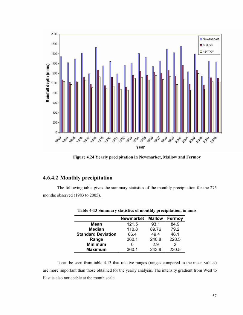
57
Figure 4.24 Yearly precipitation in Newmarket, Mallow and Fermoy
4.6.4.2 Monthly precipitation
The following table gives the summary statistics of the monthly precipitation for the 275
months observed (1983 to 2005).
Table 4-13 Summary statistics of monthly precipitation, in mms
Newmarket Mallow Fermoy
Mean 121.5 93.1 84.9 Median 110.8 89.76 79.2
Standard Deviation 66.4 49.4 46.1 Range 360.1 240.8 228.5 Minimum 0 2.9 2 Maximum 360.1 243.8 230.5
It can be seen from table 4.13 that relative ranges (ranges compared to the mean values)
are more important than those obtained for the yearly analysis. The intensity gradient from West to
East is also noticeable at the month scale.

58
Monthly precipitations were ranked into classes of 10mms in order to plot the rainfall
depth versus its density (see histograms in figure 4.25). Even if the plotted histograms are not
perfectly smooth, they can be fitted with “gamma-shaped” distribution. When depth densities in
Mallow and Fermoy show good agreement with Gamma function distributions, data in Newmarket
could not be fitted with such a probability distribution because of the too high density
corresponding to the 0-10 mms events. A logistic distribution showed better results. The Gamma
(G) and Logistic (L) distributions are respectively defined as follow:
)(),,(
/1
ab
exbaxG
a
bxa
Γ=
−
(4.1)
baxebaxL
/)(1
1),,(
−−+= (4.2)
Table 4-14 Monthly depth curve fitting and their parameters
Gauge location Probability distribution a b
Newmarket Logistic 116.8 37.2
Mallow Gamma 2.97 28.46
Fermoy Gamma 2.82 30.05
Monthly variations in depth in the mean were also studied (see figure 4.26). Good
agreement in standard deviation show that the general trend observed in figure 4.26 is a good
representation of monthly variation through a complete year. As highlighted in many rainfall
studies in Ireland (Dufour, 1995), the Irish weather exhibits few striking differences between
summer and winter time, but still have a generally observed trend, with important depths from
October to February and a lowest intensity period in between.

59
Figure 4.25 Histograms of monthly precipitation with fitted "gamma-shaped" distribution

60
Figure 4.26 Monthly variations in mean depth (Newmarket)
4.6.4.3 Daily precipitation
Before analysing the daily data, a choice had to be made in order to define the recording
depth below which the day is said to be without rain. It is indeed known than when using tipping
bucket raingauges (ground sources), small values can be recorded without actual rain. This mainly
happens when morning condensation is important enough to reach a volume that will make the
bucket tipping. Table 4.15 gives the proportion of small recorded values for the three stations and
shows a high occurrence of 0.1 mms recording (~10% of the total number of recorded values) for
both Newmarket and Mallow. It was therefore decided to neglect the 0.1 mms values and calculate
the 0.2 mms tipping occurrence (see table 4.16).
Table 4-15 Occurrence of small recording values (0.1 and 0.2 mms)
0.1 mms 0.2 mms Number of records Percentage Number of records Percentage
Newmarket 705 11.4 957 15.5 Mallow 479 8.6 818 14.6 Fermoy 265 5.5 497 10.2
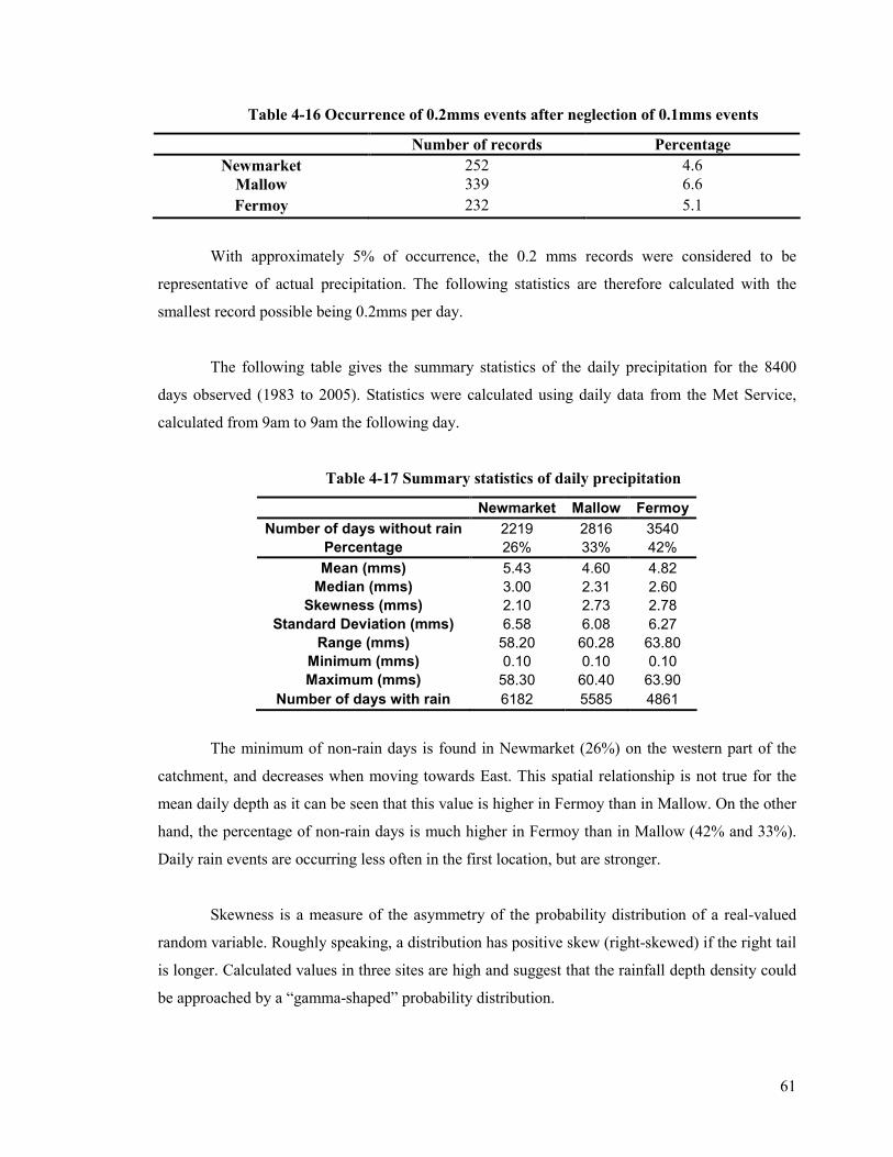
61
Table 4-16 Occurrence of 0.2mms events after neglection of 0.1mms events
Number of records Percentage Newmarket 252 4.6 Mallow 339 6.6 Fermoy 232 5.1
With approximately 5% of occurrence, the 0.2 mms records were considered to be
representative of actual precipitation. The following statistics are therefore calculated with the
smallest record possible being 0.2mms per day.
The following table gives the summary statistics of the daily precipitation for the 8400
days observed (1983 to 2005). Statistics were calculated using daily data from the Met Service,
calculated from 9am to 9am the following day.
Table 4-17 Summary statistics of daily precipitation
Newmarket Mallow Fermoy
Number of days without rain 2219 2816 3540
Percentage 26% 33% 42%
Mean (mms) 5.43 4.60 4.82
Median (mms) 3.00 2.31 2.60
Skewness (mms) 2.10 2.73 2.78
Standard Deviation (mms) 6.58 6.08 6.27
Range (mms) 58.20 60.28 63.80
Minimum (mms) 0.10 0.10 0.10
Maximum (mms) 58.30 60.40 63.90
Number of days with rain 6182 5585 4861
The minimum of non-rain days is found in Newmarket (26%) on the western part of the
catchment, and decreases when moving towards East. This spatial relationship is not true for the
mean daily depth as it can be seen that this value is higher in Fermoy than in Mallow. On the other
hand, the percentage of non-rain days is much higher in Fermoy than in Mallow (42% and 33%).
Daily rain events are occurring less often in the first location, but are stronger.
Skewness is a measure of the asymmetry of the probability distribution of a real-valued
random variable. Roughly speaking, a distribution has positive skew (right-skewed) if the right tail
is longer. Calculated values in three sites are high and suggest that the rainfall depth density could
be approached by a “gamma-shaped” probability distribution.

62
Figure 4.27 Histogram of daily precipitation with fitted distributions

63
For the three locations, gamma and lognormal distributions were the best candidates to fit
the depth density. In the three cases, gamma distributions were producing too important densities
for the first few depths (0-2 mms). Lognormal distributions (see equation 4.3) showed better
results even if the fitting curve produced low values for rainfall depths between 5 and 20 mms (see
figure 4.27).
π2),,(
22 2/)(ln
xb
ebaxLN
bax−−
= (4.3)
Table 4-18 Parameters for daily depth lognormal fitting
Gauge location a b
Newmarket 0.74 1.64
Mallow 0.63 4.51
Fermoy 0.74 1.45
4.6.4.4 Hourly precipitation
The following hourly precipitation analysis was undertaken using the 9-months OPW
dataset, which represents 6552 hourly recorded time intervals. Table 4.19 gives the summary
statistics of the three studied stations.
Table 4-19 Summary statistics of hourly precipitation
Newmarket Mallow Fermoy
Number of hours without rain 5552 5635 5726
Percentage 84% 86% 87%
Mean (mms) 0.68 0.70 0.68
Median (mms) 0.40 0.40 0.40
Standard Deviation (mms) 0.75 0.89 0.85
Skewness (mms) 2.87 2.97 3.46
Range (mms) 6.00 6.80 7.20
Minimum (mms) 0.20 0.20 0.20
Maximum (mms) 6.20 7.00 7.40
Number of hours with rain 1000 917 826

64
As can be seen in table 4.19, the mean hourly depth values are similar in the three stations,
approximately equal to 0.7 mm/hour. Considering the gradient (from West to East) already
observed in the yearly and monthly rainfall depths, and this similarity in hourly intensities, it can
be concluded that these differences amongst global cumulative depth between West and East are
due to the duration of the rainfall events more than its intensity. It was therefore decided to run a
statistic study of wet events duration from 1-hour data. Event duration is defined as the length of a
sequence of wet hours bound by either side by at least one dry hour.
Table 4-20 Summary statistics of event duration, calculated from hourly data
Newmarket Mallow Fermoy
Mean (hrs) 2.49 2.36 2.35
Standard Deviation (hrs) 2.39 2.50 2.43
Skewness (hrs) 2.16 2.86 3.27
Range (hrs) 13 16 21
Minimum (hrs) 1 1 1
Maximum (hrs) 14 17 22
Number of events 401 388 351
As predicted, the mean value for event durations is higher in Newmarket (2.5 h hours)
than in Mallow and Fermoy (approximately 2.35 hours). This small difference (6%) is enough to
explain the higher cumulative rainfall depths recorded in the western part of the catchment.
Rainfall intensity does not significantly vary but longer event durations on the West lead to higher
cumulative depths.
With only 14 hours, the maximum event duration in Newmarket is low. Mallow and
Fermoy values are higher (respectively 17 and 22 hours) but are still lower than for example the 42
hours value calculated for Cork Airport (see Dufour, 1995). With only 9 months of analysed data,
these values can not be considered as representative as some yearly averages, but are still some
good sign that the studied period (November 2005 to August 2006) was a particularly dry one.
From figure 4.28, it can be seen that short wet events are much more frequent than longer
ones. An exponential decrease of the frequency of occurrence can be noticed. The one-hour
duration events account for nearly 60% of the total number of wet events.

65
Figure 4.28 Histogram of event durations - Mallow station
4.7 Discussion
In the first part of this chapter, a precise description of the different recording raingauges
network was made in order to list all the different data sets, its quality, availability and the
precision of the coverage. With three different sources of information (the Met Service, the OPW
and the UCC Hydromet research group), and particularly with the newly installed OPW hourly
dataset, the Blackwater catchment precipitations are well recorded in both time and space. The
long records of daily rainfall available from the Met Service are also a powerful tool to monitor
long term trends within the catchment.
In the second part, the data previously described was used to produce a precise rainfall
analysis of the catchment, in term of both intensity and spatial variation.
Observation of the 9 months period recorded by the OPW recording network (November
2005 to July 2006) showed the particularly low rainfall values recorded in this period. The year
2006 has so far been really dry, with precipitation values much lower than those usually observed
in Ireland and in the Blackwater catchment. This drought was compared to the one that occurred
all over Ireland during the summer 1976. Assessing a drought severity appeared to be a subjective
and difficult task. Depending on the chosen drought indicators, one of the two studied drought
period can be considered as being more severe than the other one. From all the studied indicators
(absolute drought, partial drought, dry spell, period of insignificant rainfall and river flow
observation), it is concluded that the 1976 and 2006 droughts are comparable. Like records from

66
1976, rainfall data from 2006 is likely to become a standard against which to compare the severity
of future droughts.
An investigation of the spatial variation of rainfall depth, with both Met Service and OPW
data showed a really neat intensity gradient between the western and eastern parts of the
catchments, with depths twice as important in the West as in the East. The relationship between
rainfall depths, longitude and elevation were clearly identified and give a good understanding of
rainfall repartition among the different part of the catchment. A particular meteorological
phenomenon, called the orographic effect was also identified as potentially responsible for a
particularly wet area in the extreme East of the catchment.
Finally, a precise statistical analysis was run with yearly, monthly, daily and hourly rainfall
depths, in three different locations in the catchment (Newmarket in the West, Mallow in the centre
and Fermoy in the East). Extracted information confirmed the West-East gradient as highlighted
before. For all different time period, depth densities were approached with “Gamma-shaped”
probability distribution, with good fitting results. Occurrence of rainfall depths appeared to follow
regular trends, with a systematic high peak for low depths, and longer tails in the high depths
direction. Good accordance between observed depths and probability distribution let us believe
that using the Blackwater rainfall data as an input of rainfall prediction model would be an
interesting further work. A one-hour rain event analysis showed that hourly intensities were not
generally more important in the West than in the East. The difference in cumulative depths
recorded between the two parts of the catchment is therefore explained by longer event durations
in the West.

67
Chapter 5 Flow data
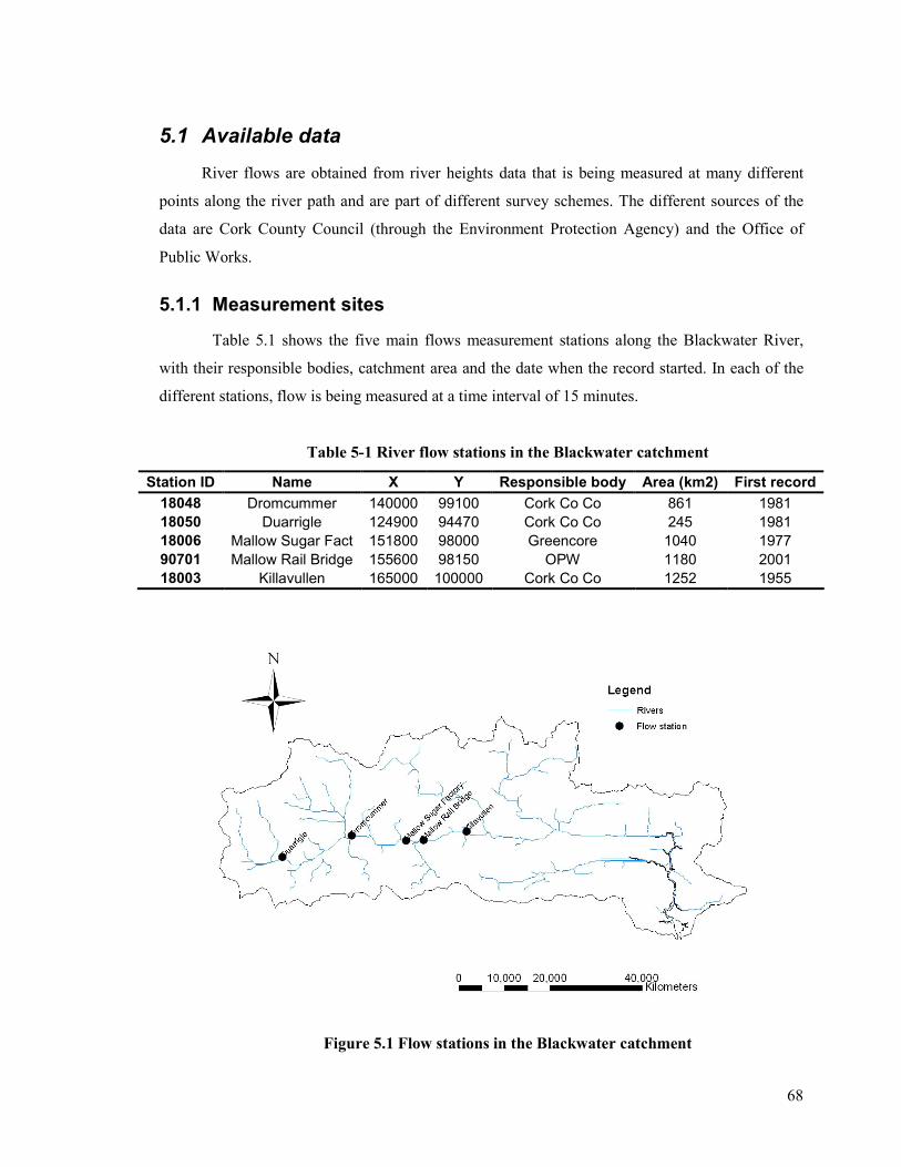
68
5.1 Available data
River flows are obtained from river heights data that is being measured at many different
points along the river path and are part of different survey schemes. The different sources of the
data are Cork County Council (through the Environment Protection Agency) and the Office of
Public Works.
5.1.1 Measurement sites
Table 5.1 shows the five main flows measurement stations along the Blackwater River,
with their responsible bodies, catchment area and the date when the record started. In each of the
different stations, flow is being measured at a time interval of 15 minutes.
Table 5-1 River flow stations in the Blackwater catchment
Station ID Name X Y Responsible body Area (km2) First record
18048 Dromcummer 140000 99100 Cork Co Co 861 1981
18050 Duarrigle 124900 94470 Cork Co Co 245 1981
18006 Mallow Sugar Fact 151800 98000 Greencore 1040 1977
90701 Mallow Rail Bridge 155600 98150 OPW 1180 2001
18003 Killavullen 165000 100000 Cork Co Co 1252 1955
Figure 5.1 Flow stations in the Blackwater catchment

69
In the following chapter of this thesis, rainfall-runoff modeling is applied to only 3 sub-
catchments: Duarrigle, Dromcummer and Killavulen. As a consequence, flow in Mallow was not
further analysed.
5.1.2 Instrumentations
Sophisticated instrumentations were installed in Duarrigle and Dromcummer in 2003, in
order to provide good data for a flood forecasting scheme in Mallow (Corcoran, 2004). Two water
level recording sensors were installed in each site in order to provide a back up system in case one
of them was to fail. Both sensors were provided by Ott-Hydrometry: the Ott-Hydrometry
Thalimedes Shaft Encoder (see figure 5.2) (Ott-Hydrometry, 2002) and the Ott-Hydrometry
Kalesto Radar Sensor (see figure 5.3) (Ott-Hydrometry, 2002).
The float-operated Thalimedes Shaft Encoder with integral data logger is designed for
continuous, unattended monitoring of water level in ground and surface waters. In the case of
changing water level, the smooth running float pulley is put into motion via the float and the float
cable, a potentiometer inside the pulley records the change and represents the change as a change
in the height on the LCD display. The change is also recorded by the inbuilt data logger.
Figure 5.2 Thalimedes shaft encoder (Ott-Hydrometry, 2004)
The Kalesto Radar Sensor is designed for continuous unattended monitoring of surface
water level. Compared with conventional level measuring systems (pressure probes, float operated
or ultrasonic systems) the installation and handling of a Radar Sensor is cost and time effective.
The Kalesto sends radar waves (microwaves) perpendicular to the water surface. These waves are
then mixed with the signals reflected on the surface. The distance travelled is then calculated
within the Kalesto and sent to the data logger.

70
Figure 5.3 Kalesto Radar Sensor (Ott-Hydrometry, 2004)
In both case, recorded water level are stored in an Ott-Hydrometry Hydrosens Multi-
Channel data logger, which can then be downloaded using a laptops, palmtops, Infra Red devices
or modem connexion.
In Duarrigle and Dromcummer, data is directly sent via telephone line and modem to two
different work stations (in UCC Hydromet Research Station, Cork and the EPA Office in Dublin)
so that the data was directly available to be used in the Mallow flood forecasting scheme
(Corcoran, 2004). The Hydras3 Pro software is used to receive the data, save it and alert the user in
case of a faulty sensor. No modem transfer system was installed in Killavullen. Data is saved in
the on-site data logger, and is collected at given time intervals.
5.1.3 Rating curves
In Duarrigle and Dromcummer data was only available in river height (meters). The river
flow can then be calculated from these values using a Rating Curve equation:
bhaQ = (5.1)
Q being the river flow in m3.s-1, h the water level in meters, a and b being dimensionless.
The EPA and the OPW have elaborated rating curves for their respective flow stations.
The coefficient a and b are obtained by extrapolation of the measured data, by plotting Q against h
(see figure 5.4). As the Rating Curve is calculated for a specific location in the river channel, the
coefficients a and b can vary very quickly from one place to another. It is then imperative to
determine a different equation for each of the 3 different stations.

71
Figure 5.4 Rating curves in Duarrigle and Dromcummer (Steinmann, 2005)
As all the points plotted on the curve are obtained by measuring the actual flow and water
level at different times, rating curves are usually plotted for low flow and normal flow conditions.
Indeed, high flow conditions (corresponding to flood flows) make measurements more difficult
and rarely happen. Low flow points are plotted and extrapolated to obtain the rating curve equation
that will be applied to a wider range of flow. The rating curves are consequently considered less
accurate for high flows than for low flow. a and b are considered reliable for the all range of flow
encountered by the river.
As the data from Killavullen flow station was directly available in cubic meters, a rating
curve was not used for this location.
5.1.4 Period of availability
Flows in Killavullen were measured since 1955 and represents consequently a very strong
database. The recording periods in Duarrigle and Dromcummer, even if starting only in 1982
provides enough data for the further modelling.
Table 5-2 Period of availability of the three flow stations
Killavullen Duarrigle Dromcummer
Opening Date October 1955 January 1982 January 1982

72
Missing data, even if infrequent in all the three stations, were encountered and replaced with
linear interpolation. Flow interpolation is an easy task to run and gives reliable results. Flow
missing data is therefore less problematic than rainfall missing values.
Two major gaps were found in both Duarrigle and Dromcummer in the year 1987, but
appeared in times of low river height. Since the undertaken modelling is based on flood events,
these omissions were not considered as being important.
5.2 Analysis
5.2.1 River flow range in the three stations
For the 1982-2006 period, the minimum recorded flow of the River Blackwater at
Duarrigle was 0.250 m3/s on the 10th of October 2000. The maximum recorded flow is 195.4 m3/s
on the 21st of October 1988. As can be seen in figure 5.5, which displays 20 years of recorded river
flow in Duarrigle, flow uncommonly exceeds 150 m3/s (8 events in total) and reaches 100 m3/s less
than 40 times in 25 years. The mean of 8.5 m3/s illustrates a low baseflow.
For the 1982-2006 period, the minimum recorded flow of the River Blackwater at
Dromcummer was 1.36 m3/s on the 14th of May 1982. The maximum recorded flow is 319.7 m3/s
on the 7th of January 1982. As can be seen in figure 5.5, flow uncommonly exceeds 250 m3/s (9
events in total) but reaches 150 m3/s quite often. The flow range of 318.4 m3/s is more important
than in Duarrigle and the highest flow is more than 200 hundred times the lowest value.
For the 1955-2006 period, the minimum recorded flow of the River Blackwater at
Killavulen was 1.6 m3/s on the 16th of September 2003. The maximum recorded flow is 602.7 m3/s
on the 2nd of November 1980. As can be seen in figure 5.5, flow uncommonly exceeds 300 m3/s
(10 events in total) but easily reaches 250 m3/s. The flow range of 601.1 m3/s can be considered as
being very important, and forebodes major issues when floods occur.
Table 5-3 Summary statistics of river flows (m3/s)
Duarrigle Dromcummer Killavullen
Min 0.25 1.36 1.6
Max 195.5 319.7 602.7
Mean 8.56 28.74 34.1
Median 4.88 17.26 22.9
Standard Deviation 11.38 33.95 35.85
Range 195.25 318.4 601.1
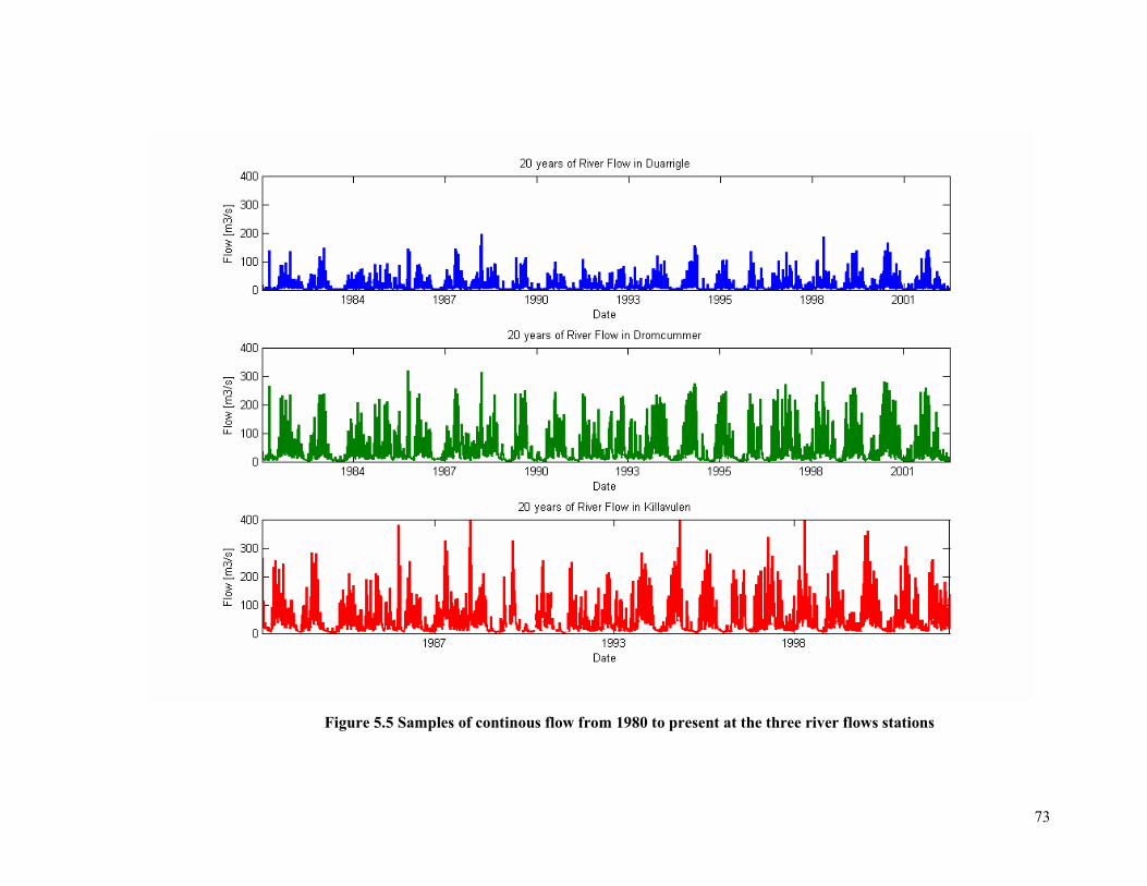
73
Figure 5.5 Samples of continous flow from 1980 to present at the three river flows stations

74
5.2.2 Data comparison
5.2.2.1 Lag time
As the River Blackwater flows from West to East, flows increase in the following order:
Duarrigle, Dromcummer and Killavulen. As can be seen in figure 5.6, this difference in flows is
observable for both baseflow and stormflow. Baseflow, which roughly is the river flow when no
surface runoff of water table recharge is occurring, is a function of the river geometry at each site.
Stormflows (which occur after high precipitation) are much higher in Dromcummer and Killavulen
than in Duarrigle.
Figure 5.6 Samples of continuous flow for one year (2001) at the three river flow
stations
When looking at a finer scale, a lag time is observable between the three stations. River
flow first reaches its peak in Duarrigle, then in Dromcummer and finally in Killavulen. Figure 5.7
compares the flood event that occurred on the 27th May 1995 at the three sites. It can be seen that
the peak occurs first in Duarrigle (~40 m3.s-1), then 2 hours later in Dromcummer (~95 m3.s-1) and
after another 5 hours in Killavulen (~115 m3.s-1). It is also clear that the hydrograph peak in
Duarrigle is much narrower than in Dromcummer, which also is narrower than in Killavulen.
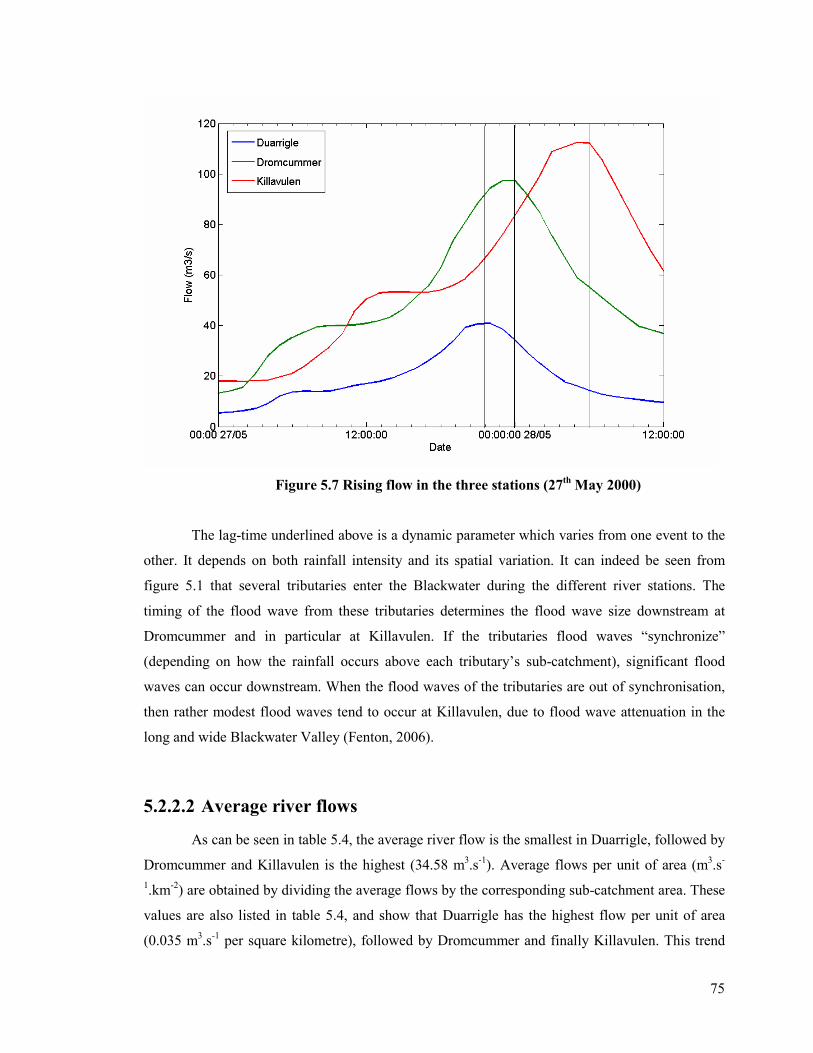
75
Figure 5.7 Rising flow in the three stations (27th May 2000)
The lag-time underlined above is a dynamic parameter which varies from one event to the
other. It depends on both rainfall intensity and its spatial variation. It can indeed be seen from
figure 5.1 that several tributaries enter the Blackwater during the different river stations. The
timing of the flood wave from these tributaries determines the flood wave size downstream at
Dromcummer and in particular at Killavulen. If the tributaries flood waves “synchronize”
(depending on how the rainfall occurs above each tributary’s sub-catchment), significant flood
waves can occur downstream. When the flood waves of the tributaries are out of synchronisation,
then rather modest flood waves tend to occur at Killavulen, due to flood wave attenuation in the
long and wide Blackwater Valley (Fenton, 2006).
5.2.2.2 Average river flows
As can be seen in table 5.4, the average river flow is the smallest in Duarrigle, followed by
Dromcummer and Killavulen is the highest (34.58 m3.s-1). Average flows per unit of area (m3.s-
1.km-2) are obtained by dividing the average flows by the corresponding sub-catchment area. These
values are also listed in table 5.4, and show that Duarrigle has the highest flow per unit of area
(0.035 m3.s-1 per square kilometre), followed by Dromcummer and finally Killavulen. This trend

76
tends to illustrate the fact that the western parts of the catchment drain more runoff to the river
network than in the East. This observation is linked with the previous highlighted gradient of
rainfall intensities from West to East (see chapter 4).
Table 5-4 Average flows in the three stations
Average river flow
(m3.s-1)
Sub-catchment area
(km2)
River flow per unit of area
(m3.s-1.km-2)
Duarrigle 8.58 245 0.035
Dromcummer 27.11 861 0.031
Killavulen 34.58 1252 0.027

77
Chapter 6 Unit Hydrograph based
Rainfall-Runoff Modelling

78
6.1 General description of an hydrograph
Before beginning to analyse a streamflow hydrograph, which describes the time history of
the changing rate of flow from a catchment due to a rainfall event rather than just the peakflow, it
is an essential step to appreciate some of the hydrograph’s main components (Shaw, 1994). The
discharge hydrograph is obtained from continuously recorded river stages and the rating curve
relationship appropriate to the specified river station (see Chapter 5). Figure 6.1 shows an example
of a flood hydrograph and its rain event.
The hydrograph (plotting of the discharge against the time) has two main components: the
area under the hump, called direct response runoff (or surface runoff), and the horizontal-like line
near the time axis representing the baseflow, i.e. the part of the flow contributed from
groundwater.
At the beginning of the rain event, the flow is only composed of the baseflow part. A period
of time elapses before the flow begins to rise (period when the rainfall is intercepted by the
vegetation, fills the soil surface cavities and makes up the soil-moisture deficits). Once the surfaces
and soils are saturated, the effective rainfall starts to contribute to flow as surface runoff: this part
of the hydrograph is called the rising limb. The peak, at the top of the hydrograph occurs when the
effective rainfall contribution is cancelled. The recession curve is the part of the curve that joins
the inflection point to the baseflow line at the inflection point. Even if there are many different
methods to determine the lag time, i.e. the catchment response time, the most commonly used is to
measure the difference between the centroids of the net rainfall hyetograph and the hydrograph.
The time of concentration can de defined as the difference in time between the end of the net
rainfall hyetograph and the end of the recession curve.
6.2 The Unit Hydrograph general theory
6.2.1 Definition
First introduced by Sherman (1932), the Unit Hydrograph (UH) is the hydrograph that results
from 1 unit depth of rainfall excess generated uniformly over the watershed at a uniform rate
during a specified period of time. The UH theory relies on three basic assumptions (Shaw, 1994):

79
Figure 6.1 Rainfall hyetograph and hydrograph, 30th November 2000, Duarrigle
• Linearity: there is a direct proportional relationship between the effective rainfall and the
surface runoff.
• Invariance: the relationship mentioned above does not change with time
• Superposition: runoff hydrographs derived for successive rain events can be summed to
obtain the total runoff hydrograph.

80
6.2.2 Convolution
Once the UH is available for a given catchment, using these three principles of linearity,
invariance and superposition, once the UH is available for a given catchment, it is possible to
derive the surface runoff hydrograph for any rainfall event. The process by which the effective
rainfall is transformed into direct runoff is called the convolution. Analytically speaking,
convolution is referred to as the theory of linear superposition (McCuen, 2004) and conceptually, it
is a process of multiplication, translation with time and addition. It can be used for processes with
either a discrete or continuous distribution function. In discrete form, which is the form used in
hydrology, the convolution equation is:
∑=
−=t
i
itUixty0
)().()( (6.1)
where x is the net rainfall distribution, y the direct runoff and U the UH.
The first burst of net rainfall of duration D is multiplied by the ordinates of the UH. The
UH is then translated for a time length of D, and the next burst of net rainfall is multiplied by the
UH. After the UH has been translated for all bursts of net rainfall of duration D, the total surface
runoff hydrograph is obtained by summing the results of all the multiplications.
6.2.3 The S-Hydrograph method
As a UH is determined for a given net rainfall duration, it is important to have a method
that transforms a d1-UH into a d2-UH (where d1 and d2 are different durations): the S-
Hydrograph method can be used for this. An S-Hydrograph is the total hydrograph resulting from
a series of continuous uniform-intensity storms delivering 1 mm in dt on the catchment. It is
obtained by summing an infinity of dt-UH, all of them separated by dt in time. A dt2-UH can be
obtained from a dt1-S-Hydrograph by subtracting the dt1-S-Hydrograph dt2 shifted S-Hydrograph,
and multiply the result by dt1/dt2. For more details, refer to Engineering Hydrology (Wilson,
1990, pp 160).
6.2.4 Catchment average UH
Each particular rain event results in a unique hydrograph, which shape can vary even if the
duration of effective rainfall is similar It is necessary to build an average catchment unit
hydrograph that can be used to forecast the discharge flow for any given rainfall hyetograph.
Average UHs were obtained in this thesis using the Aligned Peaks Method (Boorman, 1981) in
which the highest values of each rain event’s UH are aligned before the averaging.

81
Even if catchment average UH gives less accurate predictions of time to peak and peak flow rates
than an UH that was developed with an intensity that was close to the average intensity of the test
event (Kilgore, 1997), the averaging process is a necessary step that has to be carried in order to
obtain an UH that may be applicable to the widest range of rainfall events and antecedent soil
moisture conditions.
6.3 Four different approach to the unit hydrograph
6.3.1 The Rainfall-Excess Reciprocal method
The first and simplest Unit Hydrograph approach is the Rainfall-Excess Reciprocal (RRR)
method (McCuen, 2004), is to be used only with simple storm event, in which the storm
hydrograph has a smooth shape. The T-hour UH is computed by multiplying each ordinate of the
direct-runoff hydrograph by the reciprocal of the depth of rainfall excess, which equals the depth
of direct runoff (McCuen, 2004). Since the UH must have a depth of 1mm and the direct-runoff
hydrograph has a volume equivalent to the depth of rainfall excess, the reciprocal of the depth of
rainfall excess can be used as a proportionality constant to convert direct-runoff hydrograph to a
UH.
This basic determination method should only be used as a first step in modelling to give an
idea of the UH application.
6.3.2 The ordinate least-squares regression method
The least-squares regression procedure is a well known mathematical tool used in many
fields, and even if it has some limitations, its application to the UH determination has been proved
to be very convenient (Boorman, 1981). The underlying criterion in this method consists of the
minimization of the sum of the squares of the difference between the measured data and the
calculated values (Brutsaert, 2005). These differences are called the residuals and are noted iε .
The usual way of deriving the least-squares solution U is to express the linear convolution
equation that links excess rainfall, UH ordinates and direct runoff response as some matrix
equations.
∑=
+−=i
k
kki uxyi1
1. is then rewritten as Y = X . U where X, U and Y are respectively the excess
rainfall matrix, the UH ordinates and the direct runoff response. If the excess rainfall input is

82
composed with p bursts, the direct runoff response with m ordinates, the size of the UH is
1+−= pmn and the matrixes X, U and Y are constructed as follows:
=
−
−
−
p
p
p
pp
p
x
x
x
xxx
xx
x
xx
x
X
0000
.000
...00
...0
..
...
0....
00..
000
0000
1
21
11
2
12
1
,
=
−
n
n
u
u
u
u
U
1
2
1
.
. and
=
−
m
m
y
y
y
y
Y
1
2
1
.
. (6.2-4)
The matrix X having a strictly positive rank, it is reversible and the matrix 1−X therefore
exists.
When X and Y are known, the solution U is obtained by writing YXXXU tt ..).( 1−= .
This UH derivation is applicable to a wide range of rain events and can be written in a
Matlab (Mathworks, date) code in order to make the calculations easier. Finally, application of the
least-squares method to derive a UH from an observed event often produces an unrealistic solution
(UH showing oscillation or negative values) and therefore has to be smoothed in order to provided
an acceptable shape. The smoothing process is done by temporarily fixing the UH extremities to
null values, and by running a neighbour to neighbour averaging coupled with a shifting operator.
Figure 6.2 shows an example of a smoothed UH.
In the remainder of this chapter, the ordinate least-squares regression method is referred as
the ordinates method.
6.3.3 Nash Instantaneous Unit Hydrograph
The formulation of Nash’s Instantaneous Unit Hydrograph (IUH) (Nash, 1957) was
obtained under the assumption that the catchment processes from instantaneous rainfall are
equivalent to a succession of routings through linear storages (see figure 6.3). This form of IUH
has been widely applied (Raymond, 2003) due to its simplicity and efficiency.
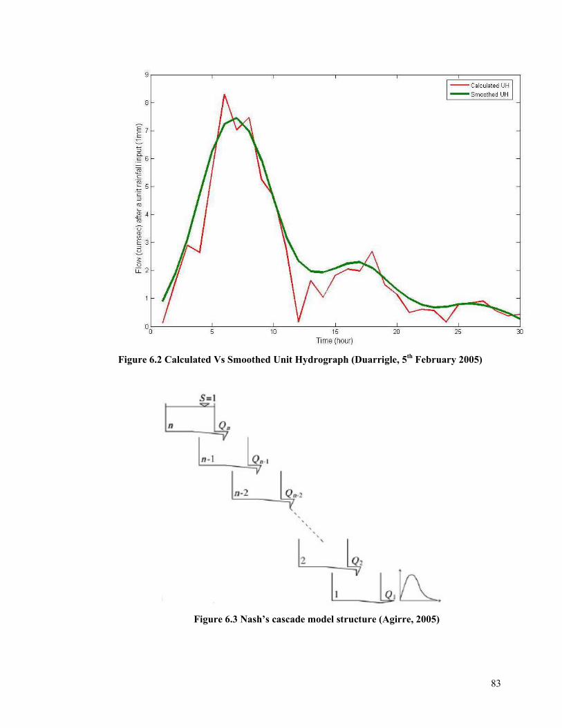
83
Figure 6.2 Calculated Vs Smoothed Unit Hydrograph (Duarrigle, 5th February 2005)
Figure 6.3 Nash’s cascade model structure (Agirre, 2005)

84
The catchment is replaced by a series of n reservoirs each having the storage
characteristics Qks .= (equation 6.5), the outflow of the upper reservoir becoming the inflow of
the next. Nash assumed that when the instantaneous input of rain ν (mms) takes place to the first
reservoir, its level is raised by an amount sufficient to accommodate the increased storage and the
discharge rises instantaneously from zero to k/ν ([S]) and diminishes with time according to the
equation:
ktek
Q /1
−=ν
(6.6)
1Q then becomes the inflow to the second reservoir in which the level diminishes according to
equation (6.6). After the rainfall input has passed through the n reservoirs, the outflow from the nth
reservoir is given by:
1/ )/()(.
−−
Γ= nkt
n ktenk
Qν
(6.7)
where )(nΓ is the gamma function equivalent to )!1( −n (for further details, see Nash, 1957).
The ordinates of the Nash IUH are obtained by replacing ν by 1mm in equation (6.7),
which leads to the gamma function equation:
1/ )/()(.
1 −−
Γ= nkt kte
nku (6.8)
This equation depends on the two parameters n (number of reservoirs) and k (storage
coefficient) which can be determined using the Momentum Method (Chow, 1988). Calculating the
1st and 2nd moments leads to the following system:
−−=+
−=
ERMknERMDRMknn
ERMDRMkn
1222
11
...2).1.(
. (6.9)
where DRM i is the ith moment of the direct runoff distribution and ERM i the ith moment of the
excess rainfall distribution.

85
An analytic solution of equation (6.9) gives the n and k parameters for a given excess
rainfall hyetograph and direct runoff hydrograph.
6.3.4 Unit hydrograph based on watershed morphology
The Geomorphological Unit hydrograph of Reservoirs (GUHR) (Lopez, 2005) which
includes the watershed structure in its formulation is based on the traditional concept which aims
to connect the watershed response to a cascade of linear reservoirs (as in the Nash IUH). The
number and size of these reservoirs is defined by the subwatershed layout along the drainage
network which leads to the geomorphologic approach of the unit hydrograph. Subwatersheds are
defined as the portions of terrain flowing to the same point of the drainage network, and are
labelled according the following numbering system (Lopez, 2005) (Figure 6.4):
• The first index starts from 1 and increases upstream, and represents channel or sub-
watershed order.
• The second order is applied to channels of the same order and increases from left to
right.
Figure 6.4 Example of the used stream ordering system (a) and its associated conceptual
reservoir model of a watershed (b) (Lopez, 2005)
It should be noted that the watershed order (maximum order of the streams within the
watershed) depends on the detail in which the drainage network is represented. Subwatersheds are
then grouped according to their order, leading the representation shown in figure (6.5).

86
Figure 6.5 Example of the used grouped stream ordering system (a) and its associated
conceptual reservoir model of a watershed (b) (Lopez, 2005)
The linear reservoir theory ( )(.)( tQktS = ) (Chow, 1988) and continuity equation are then
applied to each of the reservoirs considering a unique value for the storage coefficient k
(assumption of spatial uniformity in the watershed system). Grouping the different equations, re-
ordering its terms and resolving the obtained system leads to the following formulation:
)()().1()(
)()().1()(
)()().1()(
)()().1()(
)()().1(
112
223
1
11
tRtQkDtQ
tRtQkDtQ
tRtQkDtQ
tRtQkDtQ
tRtQkD
iii
nn
nn
n
=++−
=++−
=++−
=++−
=+
−
−−
MMM
MMM
MMM
MMM
(6.10)
where )(tQi and )(tRi are respectively the leaving flow and the intercepted rainfall of the ith
reservoir.
According to the UH theory, effective rainfall is considered to be at a constant rate and
uniformly distributed throughout the watershed. It is therefore accepted that the effective rainfall

87
depth falling over each subwatershed )(tRi depends on the ratio between the subwatershed area
iA and the total catchment area TA :
)(.)( tRA
AtR T
T
i
i = (6.11)
where t
tRT∆
=1
)( for tt ∆≤≤0 and 0)( =tRT for tt ∆≥ , t∆ being the UH duration.
The solution of the system leads to the following equation for )(1 tQ the flow at the outlet:
−−
∆= ∑ ∑
= =
−−
n
i
n
j
j
i
T
k
t
Ak
t
iA
e
ttQ
1 1
1
1 .)!1(
1.1.
1)( for tt ∆≤≤0 (6.12)
−−
∆−
−∆= ∑ ∑∑ ∑
= =
−−
= =
−∆−−
n
i
n
j
j
i
T
k
t
n
i
n
j
j
i
T
k
tt
Ak
t
iA
eA
k
tt
iA
e
ttQ
1 1
1
1 1
1)(
1 .)!1(
1..
)!1(
1..
1)( for
tt ∆≥ (6.13)
The parameter k is obtained from the effective rainfall hyetograph (ERH) and the direct
runoff hydrograph (DRH) to which are applied the Momentum Method:
∑=
−=
n
i
i
ERHDRHT
Ai
ttAk
1
.
)( (6.14)
where DRHt and ERHt are respectively the centroids of the DRH and the ERH.
The GUHR was recently developed (2005) and has been successfully tested on a small
watershed (4.7 km2) in Northern Spain. There is nonetheless no sign of its application to a large
catchment, hence its application to the study area.

88
6.4 Data processing
6.4.1 Flow separation
Hydrograph separation is an important component of the UH theory model application.
Unfortunately, there is no satisfactory technique for extracting the direct runoff hydrograph from
the total hydrograph (Beven, 2001, Bedient et al, 1992). Several techniques can be found in the
literature (see Beven 1991), however all of them lack physical justification and are arbitrary (Nash,
1960). The only physically justifiable method to estimate baseflow would be to try to estimate the
flow that might have occurred if the storm had not happened, but such a technique leads to direct
runoff hydrographs with very long tails and too complicated when applied to complex storm
events (Reed et al, 1975). Beven noted that the best method for dealing with hydrograph separation
is to avoid it all together (Beven, 2001).
Considering the lack of a reference separation technique, constancy was privileged in this
study, and the Nash method (Nash, 1960) was used in this study: a line was traced from the start of
the rising limb (A) to a point on the recession curve (B) such that the time elapsed between the end
of effective rainfall and the point B is equal to three times the lag time (see figure 6.6).
Figure 6.6 Baseflow separation using Nash’s method

89
Before deciding to choose one of the flow separation methods, a comparison between the
different available techniques was made and the results examined. Three different methods were
used:
• Graphical method: a line is traced between point A and the point of the recession curve
where the inflection occurs. This method depends on the user’s appreciation and is
therefore subjective. Nevertheless, as storm events lead to very particular hydrographs, a
visual analysis is helpful allowing the user to spot specificities.
• Area method: similar to the Nash method, the distance between A and B is 2.0AN =
where A is the catchment are in sq. miles (Ramirez, 2000). It is précised that this method is
not suitable for small catchments and should be checked for many hydrographs before
using.
• Nash’s method.
Figure 6.7 shows the different direct runoff hydrographs obtained using the three separation
methods (for the river Blackwater at Duarrigle):
Figure 6.7 Comparison of different baseflow separation method (Duarrigle)

90
Table 6-1 Comparison between Nash, Area and Graphic hydrograph separation methods
Storm
events
Date Error percentage
(Nash / Area)
Error percentage
(Nash / Graphic)
1 11 Oct 1988 1.3 5.9
2 22 Feb 1995 0.3 6.5
3 17 Nov 1997 0 11.2
4 05 Nov 1999 19.9 9.5
5 22 Dec 1999 0 2.3
6 30 Nov 2000 0.2 2.5
As can be seen in figure 6.7, differences in derived hydrograph are slight and the Nash and
Area methods’ curve are usually the same. The Graphic method always gives a smaller direct
runoff hydrograph. Table 6.1 shows the percentage of volume difference between the Nash method
and the two other alternatives. Differences are small except for the 4th event, for which the
difference in the derived direct runoff hydrograph volumes is significant (19% of difference in
volumes between the Nash and Area methods). For this particular event, the Area method leads to
a long tail hydrographs which is an undesirable characteristic. It is more acceptable to prefer the
Nash derivation that gives a more acceptable hydrograph shape. Even if the 1st event also shows a
long tail hydrograph for both Nash and Area methods, it does not appear to be a problem as the
volume under the tail is very low, which is not the case in the 4th event.
6.4.2 Rainfall separation
The aim of the rainfall separation is to partition total rainfall into infiltration losses and net
rainfall, which is the part that will be convoluted by the UH. Many different models in the past
decades have considered the concept of infiltration loss-rate curves such as the Horton infiltration
model (Chahinian, 2004), the Soil Conservation Service Curve Number method (SCS, 1972) or the
Green-Ampt equation. Later developments provided grounds for the belief that a percentage-based
method of rainfall separation was more appropriate (Houghton-Carr, 1999). In this study,
preference was given to models not intending to describe the physical processes but rather
objectively distributing the losses during the storm with recognition of the changing state of the
catchment.
This method is adapted from the original method described in the Flood Estimation
Handbook (FEH) (Institute of Hydrology, 1999) and consists in a variable loss rate changing with
antecedent wetness and conditioned so that the volumes of net rainfall and direct runoff should be

91
equal (Webster et al, 2002). In the Decreasing Proportional Loss (DPL) model, the percentage
runoff increases in proportion to the catchment wetness index (CWI) through the storm. The CWI
index is defined as follows (FEH, 1999):
SMDAPICWI −+= 125 (6.14)
where API is the Antecedent Precipitation Index and SMD the Soil Moisture Deficit.
The API, expressed in mm, is the sum of the rainfall in n preceding days weighted
exponentially such that the rainfall from the nth day has the smallest weight and the rainfall from
the preceding day has the largest weight. Its general equation is (Anctil et al, 2003):
ji
j
jti kPtAPI .)(1∑
=
−= (6.15)
where i is the number of antecedent days considered, k the exponential decay constant and dP the
rainfall on day d (mm).
The Flood Studies Report (Natural Environment Research council, 1975) and the FEH
(IH, 1999) advice a length of recession of 5 days (i.e. 5=n ) and make a modification to this
equation so that it can fit the assumption that the rainfall occurs at the centroids of each day.
Equation (6.16) is written taking into account this delay:
( )544
33
221
5.0 .... −−−−− ++++= ddddd PkPkPkPkPkAPI (6.16)
The constant k is determined assuming that the influence of the nth day’s rainfall is
reduced to approximately 1/20th of the original value ( 05.02/1 =−nk ) (Reed, 1992), leading
to 5.0=k .
The SMD is calculated using data provided by Mary Curley (Met Éireann) and computed
with the Hybrid Soil Moisture Deficit Model which has been used by Met Éireann since May
2006. The SMD is calculated on a daily basis as:
DRAINETRAINSMDSMD att ++−= −1 (6.17)
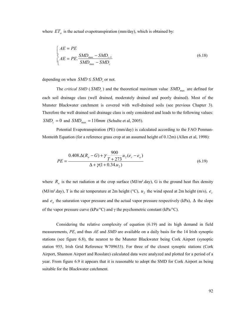
92
where aET is the actual evapotranspiration (mm/day), which is obtained by:
−
−=
=
−
c
t
SMDSMD
SMDSMDPEAE
PEAE
max
1max. (6.18)
depending on when cSMDSMD ≤ or not.
The critical SMD ( cSMD ) and the theoretical maximum value maxSMD are defined for
each soil drainage class (well drained, moderately drained and poorly drained). Most of the
Munster Blackwater catchment is covered with well-drained soils (see previous Chapter 3).
Therefore the well drained soil drainage class is only considered and leads to the following values:
0=cSMD and mmSMD 110max = (Schulte et al, 2005).
Potential Evapotranspiration (PE) (mm/day) is calculated according to the FAO Penman-
Monteith Equation (for a reference grass crop at an assumed height of 0.12m) (Allen et al, 1998):
).34.01(
)(273
900)(.408.0
2
2
u
eeuT
GR
PEasn
++∆
−+
+−∆
=γ
γ
(6.19)
where nR is the net radiation at the crop surface (MJ/m².day), G is the ground heat flux density
(MJ/m².day), T is the air temperature at 2m height (°C), 2u the wind speed at 2m height (m/s), se
and ae the saturation vapor pressure and the actual vapor pressure respectively (kPa), ∆ the slope
of the vapor pressure curve (kPa/°C) and γ the psychometric constant (kPa/°C).
Considering the relative complexity of equation (6.19) and its high demand in field
measurements, PE, and thus AE and SMD are available on a daily basis for the 14 Irish synoptic
stations (see figure 6.8), the nearest to the Munster Blackwater being Cork Airport (synoptic
station 955, Irish Grid Reference W709633). For three of the closest synoptic stations (Cork
Airport, Shannon Airport and Rosslare) calculated data were analyzed and plotted for a period of a
year. From figure 6.9 it appears that it is reasonable to adopt the SMD for Cork Airport as being
suitable for the Blackwater catchment.
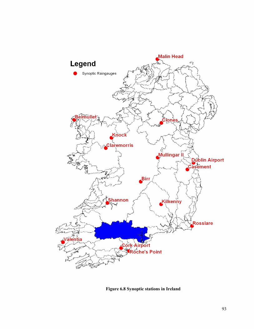
93
Figure 6.8 Synoptic stations in Ireland

94
Figure 6.9 Daily SMD values (mm/day) over the year 2005, for Cork, Shannon and Rosslare
Both API and SMD (and therefore CWI) values are calculated on a daily basis which is
not accurate enough to be used in a 1-hour step modeling. SMD and API are then readjusted by a
continuous accounting procedure through the storm event. This is done by reducing SMD by the
amount of any rain that has fallen in the previous time interval and by recalculating API as follows
(Houghton-Carr, 1999):
481
241 )5.0()5.0.(
T
t
T
tt PAPIAPI
∆
−
∆
− += (6.20)
where T∆ is the time step (usually 1 hour).
Using equations 6.21, it is then possible to calculate CWI from API and SMD at the end of
every data interval and therefore the corresponding percentage runoff for each interval:

95
=
=∑
FCWIPR
CWIrain
VolumeRunoffRapidF
ii
i
ii
*.
*
__
(6.21)
where irain and iCWI are respectively the rain and the CWI coefficient at the end of the ith data
interval.
Figure 6.10 Four examples of rainfall separation (CPL method)
As a comparison, figure 6.11 shows the application of the Phi-Index method to the same
four flood events that were plotted in figure 6.10. In this simple method, also called “constant loss
rate method”, the total rapid runoff volume is estimated and distributed uniformly across the storm
pattern, considering that the infiltration rate is constant with time. This arbitrary rate is applied
from the initiation of precipitation, and any rainfall which exceeds this rate contributes to the direct
runoff hydrograph while the reminder goes into the losses. While this technique insures that the
rainfall excess volume is exact, it does not reflect the time distribution of the effective rainfall.

96
Figure 6.11 Four examples of rainfall separation using the Phi-Index method
6.4.3 Sub-watershed delineation for the GUHR
The definition of sub-watersheds was performed using the GIS Arc Map (ESRI, date)
software. A Digital Elevation Model (DEM) with a 20 meters precision was created from
Ordinance Survey of Ireland (OSI) digital contours maps and was used to derive the drainage
network. It should be noted that the precision of the resulting drainage network depends on the
number of contributing points considered to define a stream and that this number was fixed at 1500
in this study. The sub-watersheds were then obtained from the derived drainage network and those
which had the same stream order were grouped together (see figure 6.12).

97
Figure 6.12 Geomorphological sub-watershed delineation

98
Table 6-2 Sub-watersheds areas (m2) for the 3 sub-catchments
Reservoir order Duarrigle Dromcummer Killavulen
1 4.8 32.3 51.3
2 92.6 88.7 73.3
3 35.9 77.9 71.9
4 112.2 215.4 149.1
5 --- 122.9 85.2
6 --- 159.2 121.0
7 --- 165.3 232.9
8 --- --- 183.3
9 --- --- 212.2
10 --- --- 112.2
6.5 A Graphic User Interface as an analysis tool
A Graphic User Interface (GUI) was created in the Matlab (Mathworks, 1999) platform to
run the different UH derivations (see figure 6.13). A plotting module built within this tool allows
the user to plot both the rainfall and the flow discharge distribution together, to identify the
corresponding rainfall events and peak hydrograph (see figure 6.14).
Figure 6.13 Screenshot of the developed Graphic User Interface
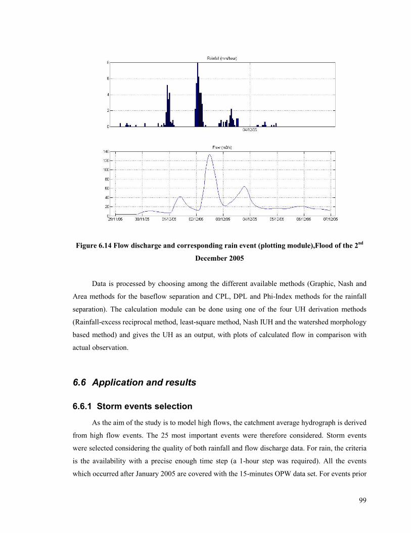
99
Figure 6.14 Flow discharge and corresponding rain event (plotting module),Flood of the 2nd
December 2005
Data is processed by choosing among the different available methods (Graphic, Nash and
Area methods for the baseflow separation and CPL, DPL and Phi-Index methods for the rainfall
separation). The calculation module can be done using one of the four UH derivation methods
(Rainfall-excess reciprocal method, least-square method, Nash IUH and the watershed morphology
based method) and gives the UH as an output, with plots of calculated flow in comparison with
actual observation.
6.6 Application and results
6.6.1 Storm events selection
As the aim of the study is to model high flows, the catchment average hydrograph is derived
from high flow events. The 25 most important events were therefore considered. Storm events
were selected considering the quality of both rainfall and flow discharge data. For rain, the criteria
is the availability with a precise enough time step (a 1-hour step was required). All the events
which occurred after January 2005 are covered with the 15-minutes OPW data set. For events prior

100
to this date, the information had to be extracted from hard-copy daily hyetograph in Met Éireann
headquarter in Dublin (see Chapter 4 – Rainfall Data). For the flow data, the shape of the direct
runoff peak was studied and selected if the peak was well defined. As can be seen on figure 6.15
and table 6.3, only 8 events were considered suitable for the catchment average unit hydrograph
construction.
Figure 6.15 The 25 highest floods in Duarrigle (selection of the suitable peaks).

101
Table 6-3 25 highest floods and those selected for the Catchment Average UH
Date River Height (m) Peak Flow discharge (m3/s) 21-Oct-88 3.818 195.5
30-Dec-98 3.714 186.9
8-Jan-05 3.464 166.9
28-Oct-04 3.462 166.7
30-Nov-00 3.439 164.9
21-Feb-82 3.416 163.1
22-Feb-95 3.327 156.3
11-Oct-88 3.324 156.1
6-Feb-84 3.212 147.6
9-Mar-95 3.202 146.8
12-Jan-88 3.169 144.3
6-Aug-86 3.167 144.2
20-Feb-02 3.114 140.3
22-Dec-99 3.095 139.0
6-Nov-00 3.094 138.8
18-Jun-82 3.083 138.0
25-Aug-86 3.050 135.7
14-Nov-03 3.043 135.1
1-Feb-02 3.042 135.1
29-Oct-96 3.040 135.0
19-Jan-88 3.034 134.5
31-Jan-83 3.032 134.4
2-Dec-05 3.020 133.5
31-Dec-00 2.986 131.1
17-Nov-97 2.979 130.6
The resulting catchment average UH is tested on floods which occurred during the period
2005-2006. Both simple and multiple peaks events with important enough direct runoff volumes
were selected.

102
6.6.2 GUHR model modification
As can be seen on figure 6.16, the original GUHR model formulation lead to poor results,
and the large size of the studied catchments (245km2 to 1292km2) was likely to be responsible.
Figure 6.16 Example of the original GUHR model in Duarrigle
It was therefore decided to keep the mathematical structure of the model (equations 6.12-
13) which is founded on acceptable theory and to modify the reservoir determination method that
did not fit the Munster Blackwater catchment. The number of reservoirs and their sizes were
directly derived from the data using an optimization process during a “calibration phase”. In order
to make the optimization process easier, two simplification morphology assumptions were made:
• The i+1th reservoir has to be greater than the ith reservoir.
• Sizes of two consecutives reservoirs are linearly related as CSS ii .1 =+ , where C is a
constant coefficient greater than 1
The optimization was first run to obtain the reservoir number and then to fix the C coefficient
(see table 6.4), which lead to the reservoir structure for each sub-catchment (see table 6.5).

103
Table 6-4 Number and size of reservoirs for the modified GUHR
Sub-catchment Number of Reservoir C
Duarrigle 5 1.325
Dromcummer 6 1.175
Killavullen 6 1.425
Table 6-5 Sub-watersheds areas (m2) for the 3 sub-catchments with the modified
GUHR
Reservoir Order
Duarrigle Dromcummer Killavulen
1 24.6 90.7 54.1
2 29.6 99.8 75.8
3 35.5 109.8 106.1
4 42.6 120.7 148.6
5 51.1 132.8 208.1
6 --- 146.1 291.3
In the remainder of this chapter, GUHR refers to the above modified GUHR.
6.6.3 Model evaluation
The simulated hydrographs are graphically observed in order to evaluate the agreement
between observed and modelled values. For a more precise evaluation, the Nash and Sutcliffe
Efficiency (NSE) indicator (Nash, 1970) was calculated:
( )
( )∑
∑
=
=
−
−
−=n
i
OBSOBSi
n
i
SIMiOBSi
NSE
1,
1
2
,,
1 (6.21)
where OBSiQ , and SIMiQ , are the observed and simulated flow values, and OBSQ the average value
of the observed flow over the full event time period.
The normalization of the variance of the observed time series of flows results in relatively
higher values of NSE in catchments with higher dynamics and lower values of NSE in catchments
with lower dynamics. An efficiency of lower than zero indicates that the mean value of the
observed time series would have been a better predictor than the model (Krause, 2005). As the
differences between the observed and predicted values are calculated as squares values, larger
values are overestimated whereas lower values are minimized. That makes the NSE an appropriate

104
efficiency indicator for flood hydrographs analysis, in which more importance is given to the flow
peak area.
Basic linear regression can also be used in order to see the correlation between the
observed and calculated time series. In this case, the slope coefficient (coefficient a if the line
equation is baxy += ) indicates the fit between the two time series (a slope coefficient equal to
one would mean that the results are perfected) and R2 (coefficient of determination) indicates the
strength of this fit.
6.6.4 Catchment Average UH derivation
The three different UH approaches (the ordinates method, the Nash IUH and the GUHR)
are applied to each of the 3 sub-catchments in the Blackwater for 8 storm events. These 8 storms
were selected for their high peak flows (among the 25 highest flows) but have different
characteristics in term of rainfall duration, peak discharge and percentage runoff, which leads to
obviously different UHs that reflect the heterogeneity of the catchment response. The 8 resulting
unit hydrographs are then averaged to obtain the catchment average UH (CAUH).
The application of each approach is shown graphically and is evaluated using the NSE
indicator.
6.6.4.1 Duarrigle
Table 6.6 lists the 8 floods used to derive the UH in Duarrigle, with the corresponding rain
event characteristics, flow response and volumes.
Table 6-6 Storm events selection in Duarrigle – CAUH derivation
Events Date rainfall duration (hours)
peak discharge (m3/s)
rainfall volume (mm)
direct runoff volume (mm)
Percentage Runoff
1 11-Oct-88 12 156.1 60.9 23.1 0.379
2 21-Oct-88 18 195.5 51.9 42.6 0.822
3 22-Feb-95 14 156.3 70.5 14.0 0.199
4 28-Oct-96 11 135.0 71.7 17.4 0.242
5 17-Nov-97 18 130.6 88.1 24.4 0.277
6 5-Nov-99 17 129.7 46.8 17.5 0.375
7 22-Dec-99 13 139.0 107.2 19.0 0.177
8 30-Nov-00 19 164.9 124.7 25.1 0.201

105
Figure 6.17 shows the application of the three different methods, in comparison with the
observed direct runoff flow. Calculated and observed values are compared in table 6.7 which also
gives NSE values for each event.
Figure 6.17 Observed and simulated direct runoff hydrographs in Duarrigle – CAUH derivation
Table 6-7 Time to peak, Peak discharge and NSE for the 8 events - Duarrigle
Observed Ordinates IUH GUHR
Events
Time to peak (hours)
Peak Discharge (m3/s)
Time to peak (hours)
Peak Discharge (m3/s)
NSE
Time to peak (hours)
Peak Discharge (m3/s)
NSE
Time to peak (hours)
Peak Discharge (m3/s)
NSE
1 14 141.23 14 129.42 0.9781 12 134.37 0.9406 13 148.65 0.8562
2 15 182.82 16 180.38 0.9962 16 182.28 0.9897 17 219.09 0.8636
3 10 130.43 11 103.17 0.7543 11 121.53 0.6896 11 111.8 0.6875
4 11 117.13 11 110.24 0.9904 9 121.75 0.9163 10 117.81 0.9157
5 15 106.79 18 103.67 0.9847 17 112.71 0.9543 18 120.49 0.9257
6 11 114.97 11 105.78 0.9725 11 128.25 0.9464 11 103.95 0.9615
7 11 120.34 11 108.37 0.9710 12 113.28 0.9629 12 100.98 0.9279
8 13 145.3 13 126.89 0.9757 12 138.99 0.9796 13 101.24 0.8181

106
Figure 6.18 Averaging the Unit Hydrograph with the 3 different methods - Duarrigle

107
Figure 6.19 3 Unit Hydrographs for Duarrigle
6.6.4.2 Dromcummer
Table 6.8 lists the 8 floods used to derive the UH in Dromcummer, with the corresponding
rain event characteristics, flow response and volumes.
Table 6-8 events selection in Dromcummer – CAUH derivation
Events Date rainfall duration (hours)
peak discharge (m3/s)
rainfall volume (mm)
direct runoff volume (mm)
PR
1 11-Oct-88 8 262.1 68.3 10.2 0.149
2 21-Oct-88 12 238.9 66.7 11.1 0.166
3 22-Feb-95 13 270.7 70.2 18.6 0.265
4 28-Oct-96 17 234.5 46.0 16.9 0.367
5 17-Nov-97 11 258.5 91.8 13.0 0.142
6 5-Nov-99 17 277.5 111.1 16.6 0.150
7 22-Dec-99 19 196.8 20.5 11.9 0.579
8 30-Nov-00 16 61.2 30.3 3.9 0.129

108
Figure 6.20 Observed and simulated direct runoff hydrographs in Dromcummer – CAUH derivation
Figure 6.20 shows the application of the three different methods, in comparison with the
observed direct runoff flow. Calculated and observed values are compared in table 6.9 which also
gives NSE values for each event.
Table 6-9 Time to peak, Peak discharge and NSE for the 8 events - Dromcummer
Observed Ordinates IUH GUHR
Events
Time to peak (hours)
Peak Discharge (m3/s)
Time to peak (hours)
Peak Discharge (m3/s)
E
Time to peak (hours)
Peak Discharge (m3/s)
E
Time to peak (hours)
Peak Discharge (m3/s)
E
1 11 187.53 11 184.46 0.9966 11 203.17 0.8814 14 162.52 0.6599
2 15 171.87 15 169.46 0.9942 12 215.26 0.8012 14 166.69 0.8016
3 17 206.38 17 204.88 0.9966 16 255.55 0.8816 20 266.51 0.6474
4 14 202.67 12 195.27 0.9460 10 243.12 0.9175 17 226.13 0.5508
5 12 184.33 13 185.92 0.9795 12 235.86 0.8008 14 181.76 0.6216
6 11 201.55 19 188.72 0.8951 14 265.44 0.7258 16 206.71 0.4696
7 21 152.4 21 152.13 0.9955 21 169.24 0.9638 23 149.96 0.8584
8 15 51.52 15 49.881 0.9987 16 44.838 0.9799 21 54.308 0.3476

109
Figure 6.21 Averaging the Unit Hydrograph with the 3 different methods -
Dromcummer

110
Figure 6.22 3 Unit Hydrographs in Dromcummer
6.6.4.3 Killavullen
Table 6.10 lists the 8 floods used to derive the UH in Killavulen, with the corresponding
rain event characteristics, flow response and volumes.
Table 6-10 events selection in Killavulen – CAUH derivation
Events Date Rainfall duration (hours)
Peak discharge (m3/s)
Rainfall volume (mm)
Direct runoff volume (mm)
Percentage Runoff
1 12-Oct-88 17 302.5 74.8 14.6 0.195
2 22-Oct-88 19 437.4 55.8 21.7 0.388
3 23-Feb-95 14 302.6 63.3 8.6 0.136
4 29-Oct-96 12 223.7 71.4 6.0 0.084
5 18-Nov-97 22 336.9 70.5 13.7 0.195
6 5-Nov-99 25 218.9 42.3 10.1 0.239
7 22-Dec-99 16 290.7 86.9 10.1 0.116
8 01-Ded-00 17 357.7 108.4 12.9 0.119

111
Figure 6.23 Observed and simulated direct runoff hydrographs in Killavulen – CAUH derivation
Figure 6.23 shows the application of the three different methods, in comparison with the
observed direct runoff flow. Calculated and observed values are compared in table 6.11 which also
gives NSE values for each event.
Table 6-11 Time to peak, Peak discharge and NSE for the 8 events - Killavullen
Observed Ordinates IUH GUHR
Events Time
to
peak
(hours)
Peak
Discharge
(m3/s)
Time
to
peak
(hours)
Peak
Discharge
(m3/s)
E Time
to
peak
(hours)
Peak
Discharge
(m3/s)
E Time
to
peak
(hours)
Peak
Discharge
(m3/s)
E
1 26 223.04 26 222.12 0.9812 18 290.68 0.6013 21 271.48 0.6799
2 21 363.67 21 331.22 0.9727 20 380.82 0.8580 23 366.54 0.8473
3 20 193.95 21 189.45 0.9747 15 214.34 0.5605 17 175.87 0.6688
4 21 130.72 22 141.77 0.9876 15 154.89 0.7251 16 118.94 0.8408
5 22 226.18 20 216.01 0.8313 20 257.91 0.6172 21 196.69 0.3543
6 21 171.26 21 166.9 0.9963 15 189.17 0.9193 19 165.91 0.8933
7 22 183.92 21 184.34 0.9868 16 227.85 0.6531 18 183.66 0.7251
8 20 226.69 20 223.48 0.9025 17 274.12 0.5067 20 232.52 0.5985

112
Figure 6.24 3 Unit Hydrographs in Killavulen

113
Figure 6.25 3 Unit Hydrographs in Killavulen
6.6.4.4 Interpretation of the results
Averaged NSE values (see table 6.12) show that the calculated direct runoff flow time
series obtained with the Ordinates Method (OM) give more accurate results than with the Nash
IUH or the GUHR. This is due to the fact that this method only uses the matrix inversion coupled
with data exploitation, and the UH construction is undertaken with the objective that its
convolution with the effective rainfall hyetograph will lead to the exact observed time series. The
slight error comes from the UH smoothing process and the NSE value would be 1 if this step was
not applied. On the other hand, this good agreement between the calculated and the observed time
series is not necessarily an advantage as the method produces poorly shaped unit hydrographs
(showing oscillation or negative values even after the smoothing process, see figure 6.18 for
example) that reflects the unrealistic nature of the solution.

114
Table 6-12 Average NSE values for the CAUH derivation phase
Ordinates Nash IUH GUHR
Duarrigle 0.9529 0.9224 0.8695
Dromcummer 0.9753 0.869 0.6196
Killavulen 0.9541 0.6801 0.701
The two other methods based on cascade of reservoirs leads to lower NSE but produces
well shaped UHs, with only slight differences between the different events (see figure 6.18 for
example), which is not the case with the Ordinates Method. The averaging process is therefore
more justifiable than in this first method. The NSE indicator results show that the Nash IUH
generally gives a greater efficiency indicator than the GUHR.
In each of the 3 sub-catchments, the CAUH obtained with the Nash IUH method has the
highest peak value and the shortest time to peak (see table 6.13). The GUHR method produces
CAUHs that appear to be between the Nash IUH and the Ordinates Method.
Table 6-13 Peak value and time to peak for the CAUH
Ordinates Nash IUH GUHR
Peak value (m3/s per unit of rainfall)
Time to peak (hours)
Peak value (m3/s per unit of rainfall)
Time to peak (hours)
Peak value (m3/s per unit of rainfall)
Time to peak (hours)
Duarrigle 7.68 5 9.14 4 6.75 5
Dromcummer 15.81 12 17.17 7 14.8 10
Killavullen 19.72 18 24.97 8 21.18 11
In order to compare the different calculated UHs on a same scale, hydrographs were
expressed in flow per unit of draining area. To do so, UHs were divided by the corresponding
catchment area in km2. Normalized average UHs are shown in figure 6.26, for each of the three
UH derivation methods.
It can be seen that the Duarrigle UH always has a significantly higher peak than the two
other stations. It can also be noted that its time to peak is smaller, and that its shape is steeper.
When important precipitations occur, the river flow in Duarrigle will respond quicker than in the
downstream stations, by rising quickly up to a high value, but lowering to its normal flow at a
same fast rate. This response type is explained by the size of the river before Duarrigle. The river
is indeed rising only 20 kilometres upstream and behaves more as a stream than a river up to this
point. With a narrow river channel (in both width and depth), and a smaller catchment area, the
contributing runoffs have higher intensities and flow is more quickly risen up.
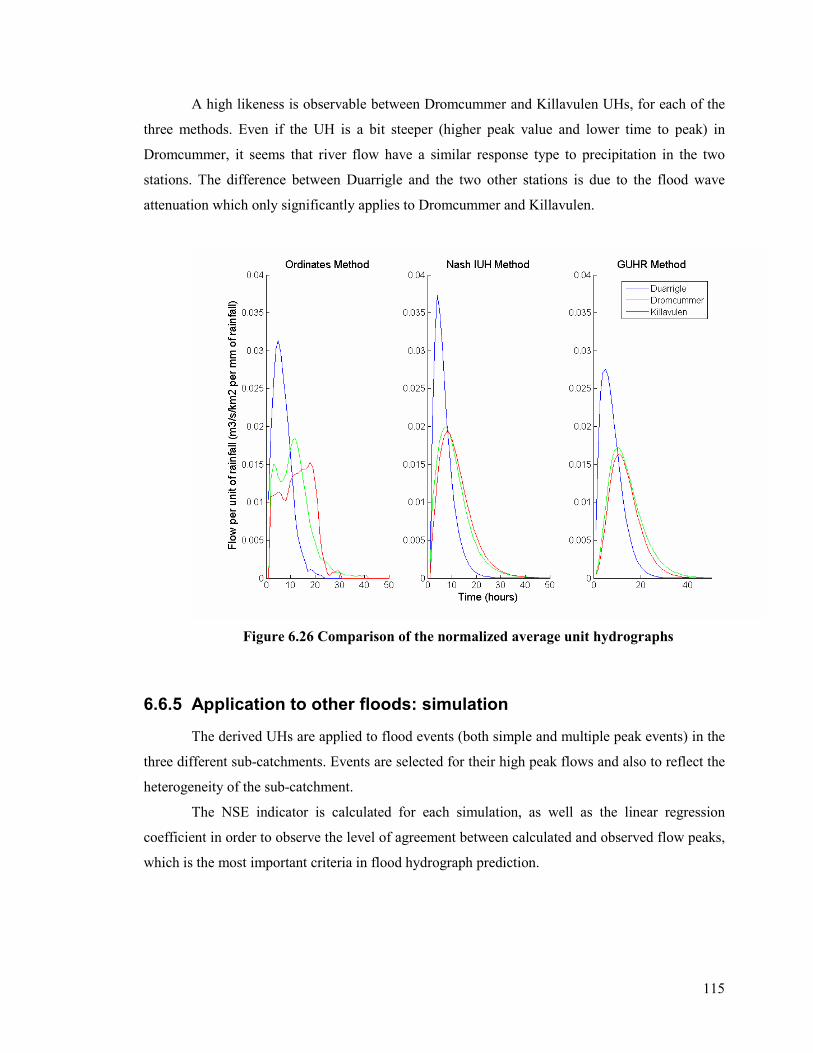
115
A high likeness is observable between Dromcummer and Killavulen UHs, for each of the
three methods. Even if the UH is a bit steeper (higher peak value and lower time to peak) in
Dromcummer, it seems that river flow have a similar response type to precipitation in the two
stations. The difference between Duarrigle and the two other stations is due to the flood wave
attenuation which only significantly applies to Dromcummer and Killavulen.
Figure 6.26 Comparison of the normalized average unit hydrographs
6.6.5 Application to other floods: simulation
The derived UHs are applied to flood events (both simple and multiple peak events) in the
three different sub-catchments. Events are selected for their high peak flows and also to reflect the
heterogeneity of the sub-catchment.
The NSE indicator is calculated for each simulation, as well as the linear regression
coefficient in order to observe the level of agreement between calculated and observed flow peaks,
which is the most important criteria in flood hydrograph prediction.

116
6.6.5.1 Duarrigle
Table 6.14 lists the 12 floods used to test the computed average UHs in Duarrigle, with the
corresponding rain event characteristics, flow response and volumes.
Table 6-14 Storm events selection in Duarrigle – Simulation
Events Date rainfall duration (hours)
peak discharge (m3/s)
rainfall volume
direct runoff volume
PR
1 22-Jan-05 18 104.5 41.5 19.6 0.471
2 12-Feb-05 63 125.4 73.2 37.6 0.514
3 30-Mar-05 9 21.1 11.6 2.9 0.253
4 6-Apr-05 47 38.5 43.0 13.5 0.314
5 17-Apr-05 16 35.8 29.7 4.1 0.140
6 28-Apr-05 14 37.9 28.7 4.5 0.158
7 27-May-05 36 56.5 59.9 18.9 0.316
8 24-Jul-05 18 40.5 48.1 5.2 0.109
9 2-Dec-05 12 133.3 56.6 16.6 0.294
10 13-Jan-06 19 122.3 56.6 22.1 0.390
11 19-Apr-06 19 28.8 22.0 4.5 0.207
12 22-May-06 20 104.1 64.2 20.4 0.318
Table 6.15 and figure 6.27 gives a comparison between observed and calculated values,
regarding to the three methods. Times to peak and peak values are calculated as well as NSE
indicator.
Table 6-15 Time to peak, Peak discharge and NSE for the 12 simulated events - Duarrigle
Observed Ordinates Nash IUH GUHR
Events Time to peak (hours)
Peak Discharge (m3/s)
Time to peak (hours)
Peak Discharge (m3/s)
E Time to peak (hours)
Peak Discharge (m3/s)
E Time to peak (hours)
Peak Discharge (m3/s)
E
1 18 87.937 16 88.153 0.98244 16 91.715 0.97042 17 85.302 0.95471
2 52 110.68 55 83.774 0.56254 54 90.712 0.58758 55 80.532 0.49418
3 8 16.909 10 19.036 0.80999 10 20.541 0.80591 10 17.592 0.81021
4 8 33.1 13 32.054 0.61932 14 33.112 0.63019 14 30.884 0.54122
5 10 29.665 10 22.677 0.91298 9 23.468 0.93491 11 21.022 0.83361
6 11 32.446 10 23.966 0.89439 9 24.636 0.8822 11 22.31 0.87744
7 14 51.011 13 57.417 0.89098 13 58.454 0.89166 13 54.419 0.87784
8 16 36.6 14 26.855 0.70372 14 27.933 0.68615 14 25.558 0.78123
9 11 117.44 10 105.36 0.95826 10 113.87 0.94115 11 96.927 0.91645
10 14 104.07 17 100.85 0.8334 17 104.69 0.83236 17 99.216 0.75055
11 12 23.278 11 19.276 0.81724 11 20.151 0.8007 11 17.989 0.85759
12 15 93.839 14 90.441 0.73764 14 90.875 0.72961 18 86.899 0.61679

117
Figure 6.27 Observed and simulated flow in Duarrigle

118
Figure 6.28 Simulated and observed peak discharge (direct runoff) – Duarrigle
A rapid graphic analysis of figure 6.27 tells us that the application of the 3 CAUH gives
really good results for a range of floods events.
The convolution of multi-peaks events (events 2, 4 and 7) also shows good agreement
between the calculated and observed even if the two lowest values of NSE, are obtained for the
events 2 and 4 (see table 6.15). The results obtained for the flood event 2 are good both in
hydrograph shape and peak value but shifted in time, which leads to the low NSE value. The peak
height prediction is nevertheless still acceptable.
In each of the 12 events, the highest calculated direct runoff flow is obtained with the
Nash IUH, followed by the GUHR and eventually the ordinates method UH. The linear regression
applied to the relationship between the observed and calculated peak flows (figure 6.28) gives the
best R2 (0.9639) to the Nash IUH, followed by the ordinates UH (0.9525) and eventually the
GUHR (0.9471). The average NSE for the 12 events put the ordinates first (0.8012), almost
equaled by the Nash IUH (0.8077), both before the GUHR (0.7759).

119
6.6.5.2 Dromcummer
Table 6.16 lists the 12 floods used to test the computed average UHs in Dromcummer,
with the corresponding rain event characteristics, flow response and volumes.
Table 6-16 Storm events selection in Dromcummer – Simulation
Events Date rainfall duration (hours)
peak discharge (m3/s)
rainfall volume (mm)
direct runoff volume (mm)
PR
1 22-Jan-05 19 196.8 20.5 11.7 0.570
2 18-Apr-05 17 41.9 27.2 2.4 0.090
3 2-Dec-05 12 228.7 52.4 10.9 0.207
4 12-Feb-05 60 176.3 50.9 20.1 0.394
5 30-Mar-05 10 30.4 11.0 1.4 0.126
6 7-Apr-05 53 65.9 34.7 8.7 0.250
7 28-Apr-05 16 61.2 30.3 3.9 0.128
8 28-May-05 40 76.2 57.7 9.8 0.171
9 24-Jul-05 21 76.5 50.1 5.1 0.102
10 13-Jan-06 20 243.9 56.7 18.2 0.321
11 19-Apr-06 19 34.6 16.3 1.5 0.093
12 22-May-06 20 220.8 61.3 12.6 0.206
Table 6.17 and figure 6.29 gives a comparison between observed and calculated values,
regarding to the three methods. Times to peak and peak values are calculated as well as NSE
indicator.
Table 6-17 Time to peak, Peak discharge and NSE for the 12 simulated events, Dromcummer
Observed Ordinates Nash IUH GUHR
Events Time to peak (hours)
Peak Discharge (m3/s)
Time to peak (hours)
Peak Discharge (m3/s)
E
Time to peak (hours)
Peak Discharge (m3/s)
E
Time to peak (hours)
Peak Discharge (m3/s)
E
1 20 151.2 19 132.3 0.9054 19 145.0 0.8476 21 133.6 0.8832
2 25 30.3 19 32.7 0.4362 17 36.2 0.1221 20 31.9 0.7613
3 10 180.7 16 156.3 0.7010 12 174.2 0.8108 15 151.8 0.2070
4 58 152.6 56 100.9 0.7637 58 115.1 0.7961 61 107.6 0.7143
5 13 24.1 17 19.1 0.8854 13 21.8 0.9168 16 19.0 0.8757
6 41 54.9 18 52.4 0.7680 15 56.8 0.7601 18 50.7 0.7995
7 15 51.4 15 51.7 0.9351 14 54.0 0.8922 17 48.4 0.9441
8 32 66.1 19 80.2 0.8217 16 83.4 0.7600 20 75.4 0.9344
9 21 74.1 21 63.9 0.9017 18 70.4 0.8805 21 63.0 0.8651
10 17 204.2 18 227.3 0.8713 19 243.9 0.9110 22 219.4 0.6487
11 14 25.5 18 17.9 0.4717 19 20.2 0.5643 22 18.2 0.1212
12 16 185.3 19 166.1 0.6066 17 168.3 0.7421 20 151.9 0.1496

120
Figure 6.29 Observed and simulated flow in Dromcummer

121
Figure 6.30 Simulated and observed peak discharge (direct runoff) - Dromcummer
The difference in derived CAUH is reflected in the three different simulations as the Nash
always produces the highest peak with the lowest time to peak.
The difference in shape in the events 2 (figure 6.29) is likely to be caused from a bad
quality flow data (interpolation for example) more than by the application of the UH convolution.
Events 3 and 12 (figure 6.29) show very low NSE values because of the fact that the
recession limb of the simulated hydrographs are not steep enough. Even if underestimating, the
calculated peak flow values are nonetheless acceptable with Nash IUH (respectively 96% and 90%
of the observed values).
The low slope coefficient (0.8916) of the linear regression (figure 6.30) for the GUHR
reflects the general underestimation produced by the application of this UH.

122
6.6.5.3 Killavullen
Table 6.18 lists the 12 floods used to test the computed average UHs in Duarrigle, with the
corresponding rain event characteristics, flow response and volumes.
Table 6-18 Storm events selection in Killavulen – Simulation
Events Date rainfall duration (hours)
peak discharge (m3/s)
rainfall volume (mm)
direct runoff volume (mm)
PR
1 23-Jan-05 18.8 235.59 17.2 8.6 0.499
2 12-Feb-05 57.8 199.2 47.0 15.6 0.331
3 22-Mar-05 38.8 98.691 31.0 4.1 0.132
4 7-Apr-05 52.8 106.5 32.8 6.0 0.184
5 18-Apr-05 47.8 91.291 27.7 3.2 0.118
6 28-May-05 33.8 112.34 57.4 7.4 0.129
7 24-Jul-05 22.8 124.01 47.2 3.6 0.076
8 10-Sep-05 27.8 64.635 24 2.5 0.103
9 24-Oct-05 50.8 188.97 35.4 9.5 0.268
10 30-Oct-05 63.8 248.31 41.5 17.2 0.415
11 3-Nov-05 77.8 261.65 61.9 18.3 0.296
12 1-Jan-06 15.8 215.51 40.2 6.2 0.155
Table 6.19 and figure 6.31 gives a comparison between observed and calculated values,
regarding to the three methods. Times to peak and peak values are calculated as well as NSE
indicator.
Table 6-19 Time to peak, Peak discharge and NSE for the 12 simulated events - Killavulen
Observed Ordinates Nash IUH GUHR
Events Time to peak (hours)
Peak Discharge (m3/s)
Time to peak (hours)
Peak Discharge (m3/s)
E Time to peak (hours)
Peak Discharge (m3/s)
E Time to peak (hours)
Peak Discharge (m3/s)
E
1 26 150.6 21 143.9 0.9251 19 157.1 0.7600 21 134.9 0.8514
2 55 147.4 53 131.28 0.6300 57 130.0 0.7284 59 108.5 0.5336
3 13 66.4 22 65.216 0.7867 14 64.3 0.9506 17 55.6 0.7538
4 37 70.5 22 51.971 0.1931 16 58.4 0.4133 19 50.1 0.1094
5 16 62.2 25 48.205 0.4606 19 58.6 0.7251 21 49.8 0.3907
6 12 92.6 23 89.185 0.6045 17 93.7 0.6857 20 81.4 0.4399
7 19 104 23 62.475 0.7154 19 72.0 0.8581 21 61.8 0.6849
8 19 50.2 22 34.001 0.6497 27 32.0 0.6645 29 26.7 0.5432
9 19 129.9 23 116 0.8072 18 127.1 0.9709 20 109.4 0.7926
10 23 174.3 28 198.04 0.6890 20 182.8 0.8021 22 158.2 0.6062
11 41 158.1 38 142.7 0.7404 32 155.3 0.6342 34 132.8 0.6787
12 16 148.9 21 112.22 0.6333 15 132.9 0.9158 18 113.5 0.6233

123
Figure 6.31 Observed and simulated flow in Killavulen
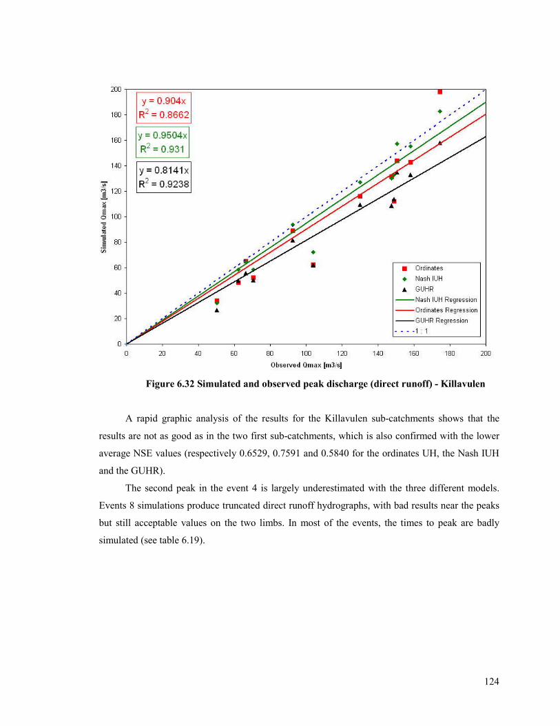
124
Figure 6.32 Simulated and observed peak discharge (direct runoff) - Killavulen
A rapid graphic analysis of the results for the Killavulen sub-catchments shows that the
results are not as good as in the two first sub-catchments, which is also confirmed with the lower
average NSE values (respectively 0.6529, 0.7591 and 0.5840 for the ordinates UH, the Nash IUH
and the GUHR).
The second peak in the event 4 is largely underestimated with the three different models.
Events 8 simulations produce truncated direct runoff hydrographs, with bad results near the peaks
but still acceptable values on the two limbs. In most of the events, the times to peak are badly
simulated (see table 6.19).
125
6.6.5.4 Interpretation of the results
The application of the CAUHs to the three nested sub-catchments shows generally good
agreement between it observed and modelled flow time series. Looking to the calculated NSE
values, it appears that the results are best for Duarrigle, good for Dromcummer and least accurate
for Killavulen (where average NSE values are respectively 0.7980, 0.7215 and 0.6654). The
accuracy of prediction decreases as the size of the catchment increases. With an average NSE close
from 0.8, results in Duarrigle (245 km2 of surface area) are considered as being good, while results
in both Dromcummer (861 km2 of surface area) and Killavulen (1292 km2 of surface area) could
be seen as reasonable. This tendency is not as obvious in the R2 slope coefficients calculated from
the linear regression applied to the relationship between observed and calculated peak flows. It can
then be concluded that the increasing error that we observed when moving to higher area
catchments mainly comes from the whole hydrograph shape and timing more than from the peak
flow value determination. The methods applied are therefore still acceptable for the prediction of
peak values.
When zooming to the sub-catchment scale, the same conclusion is made for the three areas:
Nash IUH provides the best modelling, followed by the ordinates method and the GUHR. This
conclusion comes from both graphical and indicator analysis. NSE values are indeed higher for
Nash IUH, which is also the method that produces slope coefficient (for the linear regression)
closest from 1 (see figures 1.25, 1.27 and 1.29). The Nash IUH indeed gives higher prediction than
the two other methods, which are therefore generally closer from the observed values. The
difference between the three CAUHs is more noticeable in Dromcummer (figure 6.29) and in
Killavulen (figure 6.31) than in Duarrigle (figure 6.27) where the three convolutions give similar
results. The gap is particularly important in Killavulen where the average NSE indicators are
respectively 0.7592, 0.6529 and 0.5840 for the Nash IUH, the ordinates method and the GUHR.
When results are still considered as being good with the Nash IUH, the two other methods have to
low NSE values.

126
6.7 Discussion
In this chapter, 3 different unit hydrograph methods (the ordinate least-squares method, the
Nash instantaneous unit hydrograph and the geomorphological unit hydrograph of reservoirs) were
applied to three sub-catchments of the Munster Blackwater catchment. In each sub-catchment,
three catchment average unit hydrographs (CAUH) were derived from 8 selected flood events and
were then applied to 12 other events. In both phases, baseflow and effective rainfall separation
were respectively undertaken using the Nash method (in order to have constancy in the procedure)
and the decreasing proportional loss method (in order to reflect the time distribution of the
effective rainfall).
First applications of the GUHR, which had been developed for its application to small
catchments, showed poor results in Duarrigle, Dromcummer and Killavulen. It was decided that
the original sub-watershed delineation process was not suitable for large catchments, and a
modification was therefore made, in which the different reservoirs characteristics were extracted
from the available data. An interesting work would be to test the original GUHR model on a
smaller subcatchment (approximately 10 km2) in order to test its applicability to the Blackwater
River.
During the CAUH derivation phase, the best fitting results were obtained with the ordinates
method, which only uses data exploitation and matrix inversion processes. The two other methods
are parameterized (respectively two and one parameters for the Nash IUH and the GUHR).
However, it should be noted that the ordinates method produces realistic solutions only when
applied to single peak events, and produces a high variability in term of UH shape, which makes
the averaging phase more uncertain. The two other methods show constancy in the UH derivation,
and can be applied to any kind of flood events. In the three sub-catchments, the CAUH obtained
with the Nash IUH method is greater and steeper than the two other.
The simulation phase showed that calculation lead to best results when the sub-catchment
area was smaller. Efficiency estimations indicate that results can be considered as being good in
Duarrigle, but lower in Dromcummer and Killavulen. From these results, it can be concluded that
the general UH theory should not be applied to sub-catchments draining too much important
surface area. This conclusion is in agreement with the common belief that the UH theory should
not be applied to catchments larger than 500 square kilometres (Shaw, 1994, pp433). The different
basic hypotheses made by the unit hydrograph theory are indeed more and more questionable
when the size of the studied area is growing. The assumption that the effective rainfall is constant
over the catchment and uniformly distributed in time appears to be unfounded for big catchments,
hence the low efficiency obtained for Dromcummer and Killavulen. An interesting work would be

127
to apply the same techniques to smaller sub-catchments within the Duarrigle sub-catchment, in
order to observe whether or not the results would be better.
A comparison between the three UH approaches lead to the conclusion that the Nash IUH
was the better method to be used. The results indeed showed better correlation between calculated
and observed flow time series in comparison with the ordinates and GUHR methods which
produced greater underestimations of the peak values. Calculated NSE values and linear regression
R2 make the Nash IUH the best predicting method, followed by the ordinates method and the
GUHR. This order in efficiency is also noticeable in Dromcummer and Killavulen sub-catchments,
where the Nash IUH gives best simulations for both peak flow value and time to peak. A better
understanding of the CAUH behaviour would have probably been obtained if the simulation had
been calculated for more than 12 storms. Unfortunately, the available 1hour-step data set was not
available for a long enough period of time.
Finally, it should be noted that the Ordinates method and the Nash IUF represent opposite
ends of the Unit Hydrograph theory spectrum, the former being analysis, the latter synthesis. The
Ordinates method is indeed purely based on data exploitation while the Nash IUH, with its Gamma
distribution, imposes a particular limited functional form. In the particular case of the Blackwater
River, this parametrically economic Gamma distribution proved to lead to creditable results. The
modified GUHR method, like the Nash IUH, is following a Gamma distribution, and is therefore
creating smoothed, infinite tail hydrographs. It is nevertheless positioned between the two previous
techniques, between analysis and synthesis, as its parameters are calculating through a calibration
phase that uses rainfall and flow data.

128
Chapter 7 Conclusion

129
7.1 Conclusions
With the installation of a 32 tipping bucket raingauges network in the catchment, which
provides precise time-scaled information about precipitation, the Munster Blackwater Valley has
seen its rainfall survey scheme significantly improved. From the rainfall analysis, the different
rainfall patterns and two main trends over the Munster Blackwater catchment were identified. An
intensity gradient from West to East was noticeable at all the different observations scales
(cumulative, monthly, daily and hourly rainfall). Coupled with this first factor is the impact of
elevation, which is clearly linked with higher depths of rainfall. These two relationships describe
the rainfall spatial variation, and explain some of the changes in river flows from West to East,
where flows per unit of area are lower. A particular meteorological phenomenon, called the
orographic effect was also identified as potentially responsible for a particularly wet area in the
extreme East of the catchment. The analysis also produced accurate information about the rainfall
time variation, and the way rainfall events usually occur.
Particular attention was given to the 2006 rainfall data, when significantly low values were
recorded. A drought assessment in comparison with known Irish droughts was undertaken and lead
to the conclusion that the 2006 and 1976 droughts were comparable. It was also concluded that
2006 rainfall data should be used in the future as a mean of comparison to determine the
importance of a given drought.
In the second part of the thesis, rainfall and river flow data were used as input in a rainfall-
runoff model based on different unit hydrograph approaches. The Ordinates method, purely data-
analysis-based, the synthetic Nash Instantaneous Unit Hydrograph, and the “in between”
Geomorphological Unit Hydrograph of Reservoirs (GUHR) showed good results when applied to
excess rainfall volumes. Simulated and observed river flow values were compared for a selection
of flood events, in three river stations along the Blackwater River. It was concluded, after looking
at efficiency indicators, that the parameterized Gamma distribution of the Nash Instantaneous Unit
Hydrograph was the best modelling method. This synthetic method is applicable to a wider range
of rain events than the Ordinates Method, and provides better simulation than the GUHR. A
difference was also noticeable regarding the size of the sub-catchment, and it appeared that the
three Unit Hydrograph approaches lead to better results in Duarrigle, the smallest of the three sub-
catchments, where the calculated average Nash-Sutcliffe Efficiency indicator (NSE) was
approximately 0.8. Results were still considered reasonable but lower in both Dromcummer (the
130
intermediary nested sub-catchment) and Killavulen (the largest sub-catchment), with respectively
0.72 and 0.66 as average NSEs.
Even if the Unit Hydrograph is sometimes considered as being a simple rainfall-runoff
solution, its application to the Munster Blackwater catchment showed good results in flood
hydrographs simulations. Choosing this metric approach to construct direct runoff hydrographs
from excess rainfall volumes appeared to be relevant, and suitable to the Blackwater River flow
response type. Accordance between calculated and observed values were indeed better than with
some more complicated models that have already been applied to this same catchment.
7.2 Recommendations for further research
The different analyses undertaken in this thesis have highlighted different points that should
be considered for further research. These recommendations mainly apply to the rainfall analysis,
and to the rainfall-runoff modelling effort.
7.2.1 Rainfall analysis
• At the time of the writing, rainfall data was only available up to July 2006. As the summer
2006 was a drought period, an interesting piece of research would be to run the drought
assessment with some more updated data, and to compare the results with previous
drought (e.g. 1976).
• Statistical analysis of monthly, daily and hourly rainfall showed good accordance between
observed depths and known probability distributions. It lets us believe that the Blackwater
rainfall data could be used as an input for rainfall prediction model. Particular attention
could be given to the use of an artificial neural network.
• Finally, the increasing data set of hourly rainfall could be used to explore the rainfall
disagregation, from daily or weekly data to smaller increments. If well calibrated, such a
work could significantly improve the quality of the different data sources.
7.2.2 Rainfall-Runoff modelling
• In the rainfall-runoff modelling, priority was given to rainfall separation and the Unit
Hydrograph derivation. The baseflow separation was undertaken with a widely accepted
but still simple method. Accuracy would certainly be improved by integrating a precise
module for the baseflow element that could take into account the Catchment Wetness

131
Index, the different infiltration processes and the contribution to the river channel flows
from the adjacent saturated soils.
• The application of Geomorphological Unit Hydrograph of Reservoirs, with its original
reservoirs delineation process, appeared not to be suitable for large watershed as the one
studied in this thesis (245 to 1265 km2). As it was originally developed and successfully
tested for a small catchment (4.7 km2, in North Spain), its applicability to the Blackwater
catchment should be re-considered with a smaller watershed within the Duarrigle sub-
catchment (~ 10 km2).
• The quality of the results quality from simulation with the three unit hydrograph
techniques (Ordinates method, Nash IUH and the modified GUHR) appeared to decrease
with the size of the sub-catchment. In order to comfort the idea that the Unit Hydrograph
will provide better results with smaller drainage areas, the same technique should be
applied to smaller nested sub-catchments and the upper threshold of catchment size for
unit hydrograph analysis should be delineated.
• For each of the three watersheds, the Catchment Average Unit Hydrographs were derived
from 8 events and were then applied to 12 different events for simulation purposes. These
numbers were chosen due to the sort dataset of 1-hour rainfall (from January 2005 to July
2006). A better understanding of the application of the catchment unit hydrographs will
certainly be obtained if a wider range of events could be studied.
• Finally, the investigation of built-in metric unit hydrograph based rainfall-runoff models
should be considered. A particular attention should be given to the IHACRES
(Identification of a unit Hydrograph And Component flows from Rainfall, Evaporation
and Streamflow data) that promises to give good results for the Munster Blackwater
Catchment.

132
References

133
Agirre U., Lopez J.J., Gimena F.N., Goni M., 2005. Application of a unit hydrograph based on
subwatershed division and comparison with Nash’s instantaneous unit hydrograph, Catena
64(2005), pp 321-332.
Ahmad S., Simonovic S.P., 2005. An artificial neural network model for generating hydrograph
from hydro-meteorological parameters, Journal of Hydrology 315 (2005), pp 236-251.
Allen, R.G., Pereira, L.S., Raes, D. and Smith, M. 1998. Crop evapotranspiration. Guidelines for
computing crop water requirements. FAO irrigation and drainage paper 56, 227 pages.
Anctil F., Michel C., Perrin C., Andreassian V., 2003, A soil moisture index as an auxiliary ANN
input for stream flow forecasting, Journal of Hydrology 286 (2004), pp 155-167
ASCE Task Committee on Application of Artificial Neural Networks in Hydrology, 2000.
Artificial Neural Networks in Hydrology. I: Preliminary concepts, Journal of Hydrology (2000), 2,
pp 115-123.
ASCE Task Committee on Application of Artificial Neural Networks in Hydrology, 2000.
Artificial Neural Networks in Hydrology. II: Hydrologic applications, Journal of Hydrology
(2000), 2, pp 124-137.
Bedient P.B., Huber W.C., 1992, Hydrology and Floodplain analysis, 2nd edition, New York,
Addison–Wesley Publishing Company.
Beven K.J., 2001, Rainfall-Runoff Modelling, The Primer, John Wiley and Sons, Ltd, Chichester,
England, 360pp.
Beven K.J., Kirkby M.J., 1979. A physically based, variable contributing area model of basin
hydrology. Hydrological Sciences Bulletin, 24(1), pp 43-69.
Beven K.J., 1984. Infiltration into a class of vertically non-uniform soils. Hydrological Sciences
Journal, 29(4), pp 425-434.

134
Beven K., 1989. Changing ideas in hydrology -- The case of physically-based models. Journal of
Hydrology, 105(1-2), pp 157-172.
Boorman D.B, Reed D.W., 1981. Derivation of a catchment average unit hydrograph, report 71,
Institute of Hydrology.
Brutsaert W., 2005. Hydrology, an Introduction, Cambridge University Press, pp605.
Cameron D., 2006. An application of the UKCIP02 climate change scenarios to flood estimation
by continuous simulation for a gauged catchment in the northeast of Scotland, UK (with
uncertainty), Journal of Hydrology, 328, pp 212-226.
Chahinian N., Moussa R., Andrieux P., Voltz M., 2004, Comparison of infiltration models to
simulate flood events at the field scale, Journal of Hydrology 306 (2005) pp191-214.
Yen B.C, Lee K.T, 1997. Unit Hydrograph derivation for ungauged Watersheds by Stream-Order
Laws, Journal of Hydrologic Engineering 2(1997), pp 1-9.
Chow V.T., Maidment D.R., Mays W., 1988. Applied Hydrology, McGraw-Hill International
Editions, Civil Engineering Series.
Corcoran G., 2004. Development and examination of flood warning systems for the Munster
Blackwater at Mallow. M.Eng.Sc Thesis, University College Cork, Cork, 145 pp.
Croke B., Cleridou N., Kolovos A., Vardavas I., Papamastorakis J., 2000. Water resources in the
desertification-threatened Messara Valley of Crete: estimation of the annual water budget using a
rainfall-runoff model, Environmental Modelling and Software 15(2000), pp 387-402.
Croke B., 2006. A technique for deriving an average even unit hydrograph from streamflow – only
data for ephemeral quick-flow dominant catchments, Advances in Water Resources 29 (2006), pp
493-502.
Dawson C.W., Abrahart R.J., Shamseldin A.Y., Wilby R.L., 2006. Flood estimation at ungauged
sites using artificial neural networks, Journal of Hydrology 319(2006), pp 391-409.

135
Dooge J.C., 1959. A General Theory of the Unit Hydrograph, Journal of Geophysical Research,
64(2), pp 241-256.
Dufour C., 1995. Analysis of thirty-one years of hourly rainfall at Cork, Ireland, Higher Diploma
Thesis, University College of Cork.
Fenton M., Guero P., McKeogh E., Leahy P., Kiely G., 2006. Flood Studies Update Programme,
Work Group 3 – Flood Hydrograph Analysis, Work Package 3.2, Flood Event Analysis.
Gallart F., Latron J., Llorens P., Beven K., 2006. Using internal catchment information to reduce
the uncertainty of discharge and baseflow predictions, in press, Water Resources.
Gupta V.K., Waymire E., Wang C.T., 1980. A representation of an instantaneous unit hydrograph
from geomorphology, Water Resource Research, 16(5), pp 855-862.
Houghton-Carr H., 1999, Restatement and application of the Flood Studies Report rainfall-runoff
method, Flood Estimation Handbook Volume 4, Institute of Hydrology.
Ivanov V.Y., Vivoni E.R., Bras R.L., Entekhabi, D., 2004. Preserving high-resolution surface and
rainfall data in operational-scale basin hydrology: a fully-distributed physically-based approach.
Journal of Hydrology, 298(1-4),pp 80-111.
Jakeman A.J., Littlewood I.G., Whitehead P.G., 1990. Computation of the instantaneous unit
hydrograph and identifiable component flows with application to two small upland catchments,
Journal of Hydrology, 117, pp 275-300.
Kildore L. J., 1997, Developpement and evaluation of a GIS-based spatially distributed unit
hydrograph model, Thesis submitted to the Faculty of the Virginia Polytechnic Institute and State
University
Kirkby M.J., 1975. Hydrograph modelling strategies. In: R. Peel, M. Chisholm and P. Hagget
(Editors), Processes in Physical and Human Geography. Heinemann, London, pp 69-90.

136
Kokkonen T.S, Jakeman A.J., 2001. A Comparison of metric and conceptual approaches in
rainfall-runoff modeling and its implications, Water Resources Research 37(9), pp 2345-2352.
Krause P., Boyle D.P., Base F., 2005. Comparison of different efficiency criteria for hydrological
model assessment, Advances in Geosciences, 5 pp 89-97.
Kumar S.A.R., Sudheer K.P., Jain S. K., Agarwal P.K., 2004. Rainfall-runoff modelling using
artificial neural networks: comparison of network types.
Hydrol. Processes, 2004, 19, No. 6, pp 1277-1291.
Lamb R., Beven K.J., Myrabo S., 1997. Discharge and water table predictions using a generalized
TOPMODEL formulation, Hydrological Processes, 11, pp 1145-1168.
Leahy P., Kiely G., Corcoran G., 2006. Minimal input artificial neural networks for flood
forecasting, Water Management Journal, in review.
Lee K.L., Chang C.H., 2005. Incorporating subsurface-flow mechanism into geomorphology-
based IUH modeling, Journal of Hydrology, 311 (2005), pp 91-105.
Lee K.L., Yen B.C., 1997. Geomorphology and Kinematic-Wave-Based Hydrograph Derivation,
Journal of Hydraulic Engineering, 123 (1997), pp 73-80.
Linsley R.K., Kolher M.A., Paulhus J.L.H., 1988. Hydrology for Engineers, SI Metric Edition,
McGraw-Hill Book Company.
Lopez J.J., Gimena F.N., Goni M., Agirre U., 2005. Analysis of a unit hydrograph model based on
watershed geomorphology represented as a cascade of reservoirs, Agricultural Water Management
77(2005), pp 128-143.
Lopez J.J., Gimena F.N., Goni M., Agirre U., 2005. Application of a unit hydrograph based on
subwatershed division and comparison with Nash’s instantaneous unit hydrograph, Catena 64
(2005), pp 312-332.

137
MacCárthaigh M., 1996. An assessment of the 1995 drought : including a comparison with other
known drought years, EPA, Wexford.
McCuen R.H., 2004. Hydrologic Analysis and Design, Third Edition, Pearson Prentice Hall
Editions.
McCullough W., Pitts W.H., 1943. A logical calculus of the ideas immanent in
nervous activity, Bull. Math. Biophys., 1943, 5, pp 115-133.
Nash J.E., 1957. The form of the instantaneous unit hydrograph. Int. Assoc. Sci. Hydrol. 45(3), pp
114-l 21.
Nash J.E., 1960. A unit hydrograph study, with particular reference to British catchments, Proc
Inst Civ Eng 17, pp 249-282.
Nash J.E., Sutcliffe J.V., 1970. River flow forecasting through conceptual models, Part I, A
discussion of principles, Journal of Hydrology, 10, pp 282-290.
Pedruco P., Indicative flood forecasting in Ireland, 2005. M.Sc Thesis, Imperial College of
Science, Technology and Medicine, London, 152 pp.
Rajurka M.P., Kothyari U.C., Chaube U.C., 2004. Modeling of the daily
rainfall-runoff relationship with artificial neural network. J. Hydrol., 2004, 285, pp 96-113.
Raymond I.J., Coon G.C., 2003. True Form of Instantaneous Unit Hydrograph of Linear
Reservoirs, Journal of Irrigation and Drainage Engineering, pp 11-17.
Reed D. W., 1992. Triggers to server floods: Extreme rainfall and antecedent wetness, Water
resources and reservoir engineering, Thomas Telford, London, 1992.
Rodriguez-Iturbe I., Valdes J.B., 1979. The geomorphologic structure of hydrologic response,
Water Resources Research, 15(6), pp 1409-1420.

138
Sahoo G.B., Ray C., DeCarlo E.H., 2006. Use of neural network to predict flash flood and
attendant water qualities of a mountainous stream Oahu, Hawaii, Journal of Hydrology (2006),
327, pp 525 538.
Scanlon T.M., Raffensperger J.P., Hornberger G.M., Clapp R.B., 2000. Shallow subsurface storm
flow in a headwater catchment: observations and modeling using a modified TOPMODEL, Water
Resources Research, 36, 9, pp 2575-2586.
Scanlon T.M., Kiely G., Quishi X., 2004. A nested catchment approach for defining the
hydrological controls on phosphorus transport, Journal of Hydrology, 291(3-4), pp 218-231.
Schulte R.P.O., Diamond J., Finkele K., Holden N.M. and Brereton A.J., 2005, Predicting the Soil
Moisture Conditions of Irish Grasslands. Irish Journal of Agricultural Research 44, pp 95-110.
Shaw M.S., 1994. Hydrology in Practice, Third Edition, Chapman and Hall Editions.
Sherman L.K., 1932. Stream flow from rainfall by the unit-graph method, Engrg. News Rec., 108,
pp 501-505.
Smith R.M.S, Evans D.J, Wheater H.S., 2005. Evaluation of two hybrid metric-conceptual models
for simulating phosphorus transfer from agricultural land in the River Enborne, a lowland UK
catchment, Journal of Hydrology, 304(2005), pp 366-380.
Soil Conservation Service (SCS), 1972. National Engineering Handbook, Section 4, Hydrology.
U.S. Dept. of Agriculture (available from U.S. Government Printing Office), Washington, DC.
Steinmann E., 2005. An Investigation of Flood Forecasting using a Physically-Based Rainfall-
Runoff Model, M.Eng.Sc Thesis, University College Cork, Cork, 119 pp.
Tilford K.A., Sen K., Chatterton J. B., Whitlow C., 2003. Environment Agency /DEFRA R&D
Technical Report W5C-013/5/TR.
Wagener T., Wheater H. S., Gupta H.V., 2004, Rainfall-Runoff Modeling in Gauged and
Ungauged Catchments, Imperial College Press, London, England, 306 pp.

139
Wagener T., lees M.J., Wheater H. S., 2000. Incorporating predictive uncertainity into a rainfall-
runoff modeling system. Proceedings of Hydroinformatics 2000 Conference, on CD, Iowa, USA.
Webster P., Ashfaq A., 2002, Comparison of UK flood event characteristics with design
guidelines, Water and Maritime Engineering 156 (2003), pp 33-40.
Wheater H.S., Jakeman A.J. and Beven K.J., 1993. Progress and direction in rainfall-runoff
modelling. In: A.J. Jakeman, M.B. Beck and M.J. McAleer (Editors), Modelling change in
environmental systems. John Wiley & Sons, pp. 101-132.
Wilson E.M., 1990. Engineering Hydrology, Fourth Edition, McMillan Education Ltd Editions.

140
Appendix A
Matlab Code for the rainfall and baseflow separation
%[RF,effective_rain]=RAINFALL_SEPARATION(R,F,flow_points,rain_points)
%INPUT
%stat=duar/drom/kill
%R=rainfall data vector
%F=flow data vector
%flow_points=start of the rising limb, peak, end of the runoff
hydrograph
%rain_points=start and en of the rain event
%OUTPUT
%RF= Response Flow
%effective rain=rain – losses
function
RF,effective_rain]=RAINFALL_SEPARATION(R,F,flow_points,rain_points)
if stat=='duar'
cd 'C:\matwork\duarigle';
load ('duar_rain.mat');
rain_stat=rain_duar;
cd 'C:\matwork\duarigle\OPW'
load UH_IUH.mat
area=245;
elseif stat=='drom'
cd 'C:\matwork\drom';
load ('drom_rain.mat');
rain_stat=rain_drom;
cd 'C:\matwork\drom\OPW'
load UH_IUH.mat
area=861;
elseif stat=='kill'
cd 'C:\matwork\killavulen';
load ('kill_rain.mat');
rain_stat=rain_kill;
cd 'C:\matwork\killavulen\OPW'

141
load UH_IUH.mat
area=1292;
end
%x=[x1,x2,x3]=start,peak,end
[flow_points(1,3).Position(1),flow_points(1,2).Position(1),flow_points(1
,1).Position(1)];
%Y=[y1,y2]
Y=[flow_points(1,3).Position(2),flow_points(1,2).Position(2),flow_points
(1,1).Position(2)];
%--------- LAG TIME -----------------------------------
r1_date=rain_points(1,2).Position(1,1);r1=floor(r1); %time of first rain
r2_date=rain_points(1,1).Position(1,1);r2=floor(r2); %time of last rain
r1= (r1_date - R(1,1)) / (1/24) +2; %index of R where the first rain is
r2= (r2_date - R(1,1)) / (1/24) +1; %index of R where the last rain is
%rain is extracted from R
for i=r1:r2
rain(i-r1+1,1)=R(i,1);
rain(i-r1+1,2)=R(i,2);
end
%rain_centroid : = (t1rain1 + t2rain2 + t3rain3 + ...) /
(rain1+rain2+rain3+...)
%(centroid is a kind of barycenter)
for i = 1 :length(rain)
tR(i) = rain(i,1)*rain(i,2);
end
rain_centroid= (sum(tR)) / (sum(rain(:,2)));
rain_centroid= floor( rain_centroid/(1/24) ) * (1/24);
for i=1:length(R)
if datestr(F(i,1),'dd-mmm-yyyy
HH:MM:SS')==datestr(rain_centroid,'dd-mmm-yyyy HH:MM:SS')
rain_centroid_index=i;break
end
end
%lag time = (flow peak) - (rain centroid)
LAG = flow_points(1,2).Position(1) - rain_centroid;

142
LAG = floor( LAG/(1/24) )* (1/24); % to make it multiple of (1/24 JD = 1
hour)
%1 index unit = 1 hour = 1/24 JD
LAG_index= LAG / (1/24);
end_index=r2 + 4*LAG_index;
%---------------------------------------------------------------
xi=[flow_points(1,3).Position(1):1/24:F(end_index,1)];%every hour
between x1 and x2
if xi(end)~=F(end_index,1) %because of the approximation 1/24=0.0417
xi=[xi,F(end_index,1)];
end
x=[flow_points(1,3).Position(1),F(end_index,1)];
Y=[flow_points(1,3).Position(2),F(end_index,2)];
yi = interp1(x,Y,xi); %interpolates the line between the two points =
baseflow
resp_flow=zeros(length(F),2);
for i=1:length(F) %date
resp_flow(i,1)=F(i,1);
end
%resp_flow=the peak with the whole time period
%RF=the peak only
for i=[flow_points(1,3).DataIndex:end_index]
resp_flow(i,2)=F(i,2)-yi(i-flow_points(1,3).DataIndex +1);
RF(i-flow_points(1,3).DataIndex+1,1)=resp_flow(i,1);
RF(i-flow_points(1,3).DataIndex+1,2)=resp_flow(i,2);
end
%flow_centroid : = (t1RF1 + t2RF2 + t3RF3 + ...) / (RF1+RF2+RF3+...)
for i = 1 :length(RF)
tRF(i) = RF(i,1)*RF(i,2);
end
RF_centroid= (sum(tRF)) / (sum(RF(:,2)));
RF_centroid= floor( RF_centroid/(1/24) ) * (1/24);
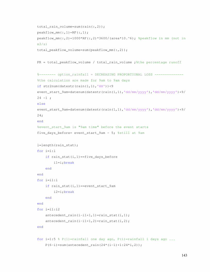
143
total_rain_volume=sum(rain(:,2));
peakflow_mm(:,1)=RF(:,1);
peakflow_mm(:,2)=1000*RF(:,2)*3600/(area*10.^6); %peakflow in mm (not in
m3/s)
total_peakflow_volume=sum(peakflow_mm(:,2));
PR = total_peakflow_volume / total_rain_volume ;%the percentage runoff
%-------- option_rainfall = DECREASING PROPORTIONAL LOSS --------------
%the calculation are made for 9am to 9am days
if str2num(datestr(rain(1,1),'HH'))<9
event_start_9am=datenum(datestr(rain(1,1),'dd/mm/yyyy'),'dd/mm/yyyy')+9/
24 -1 ;
else
event_start_9am=datenum(datestr(rain(1,1),'dd/mm/yyyy'),'dd/mm/yyyy')+9/
24;
end
%event_start_9am is "9am time" before the event starts
five_days_before= event_start_9am - 5; %still at 9am
l=length(rain_stat);
for i=1:l
if rain_stat(i,1)==five_days_before
i1=i;break
end
end
for i=i1:l
if rain_stat(i,1)==event_start_9am
i2=i;break
end
end
for i=i1:i2
antecedent_rain(i-i1+1,1)=rain_stat(i,1);
antecedent_rain(i-i1+1,2)=rain_stat(i,2);
end
for i=1:5 % P(1)=rainfall one day ago, P(i)=rainfall i days ago ...
P(6-i)=sum(antecedent_rain(24*(i-1)+1:24*i,2));

144
end
%API5 is the API5 value on the starting day at 9am
API5=0.5*(P(1)+0.5*P(2)+(0.5.^2)*P(3)+(0.5.^3)*P(4)+(0.5.^4)*P(5));
API=[];
l=length(rain_stat);
for i=1:l
if rain_stat(i,1)==event_start_9am
i3=i;break
end
end
%------------------------------------------------------------------
R1=rain_points(1,2).Position(1,1);
start_rain_fixed=floor(R1)+floor((R1-floor(R1))/(1/24))*1/24;
R1=start_rain_fixed;%time of first rain FIXED
R2=rain_points(1,1).Position(1,1);
enddate_rain_fixed=floor(R2)+floor((R2-floor(R2))/(1/24))*1/24;
R2=enddate_rain_fixed;%time of last rain FIXED
%------------------------------------------------------------------
for i=i3+1:l
if abs(rain_stat(i,1)-R2)<1/1440
i4=i;break
end
end
API(1,1)=event_start_9am;
API(1,2)=API5;
smd(1,1)=event_start_9am;
smd(1,2)=SMD( datestr(event_start_9am,'dd/mm/yyyy') );
for i=i3+1:i4
API(i-i3+1,1)=rain_stat(i,1);
API(i-i3+1,2)=API(i-i3,2)*(0.5.^(1/24))+rain_stat(i-
1,2)*(0.5.^(1/48));
smd(i-i3+1,1)=rain_stat(i,1);
smd(i-i3+1,2)=max(smd(i-i3+1-1,2)-rain_stat(i,2),0);
end
for i=i3:i4
RR(i-i3+1,1)=rain_stat(i,1);
RR(i-i3+1,2)=rain_stat(i,2);
CWI(i-i3+1,1)=API(i-i3+1,1);

145
CWI(i-i3+1,2)=125+API(i-i3+1,2)+smd(i-i3+1,2);%CWI= API + 125 (+SMD)
RCWI(i-i3+1,1)=API(i-i3+1,1);
RCWI(i-i3+1,2)=CWI(i-i3+1,2)*RR(i-i3+1,2);
end
Fa= total_peakflow_volume / (sum(RCWI(:,2))) ;
for i=1:length(CWI)
PR2(i,1)=CWI(i,1);
PR2(i,2)=CWI(i,2)*Fa;
end
for i=1:length(CWI)
if CWI(i,1)==rain(1,1)
i5=i;break
end
end
for i=i5:length(PR2)
effective_rain(i-i5+1,1)=PR2(i,1);
effective_rain(i-i5+1,2)=PR2(i,2)*RR(i,2);
infiltration(i,2)=(1-PR2(i,2))*RR(i,2);
end

146
Appendix B
Matlab code for the event Unit Hydrograph Derivation
%function DER stands for (UH) derivation
%stat=duar/drom/kill
%RF=Response flow=direct runoff
%effective_rain=rainfall - losses
%OUTPUT=UNIT HYDROGRAPH with OR ,Nash IUH and GUHR
function [U_ord,U_nas,U_mor]=DER(stat,RF,effective_rain)
%UNIT HYDROGRAPH DERIVATION = ORDINATES METHOD ------------------------
Y=RF(:,2);
p=length(effective_rain); %p=number of rainfall imputs
m=length(Y); %m=length of the peak hydrograph
n=m-p+1; %n=size oh the UH
X=zeros(m,n);
%convolution
for j=1:n
for i=1:p
X(i+j-1,j)=effective_rain(i,2);
end
end
U=inv(X'*X)*X'*Y;%U=Unit hydrograph, obtained by the least square method
UH_ord=U;
YY=X*UH_ord;
uh=U;
%smoothing process
uh_smoo=[0;uh;0];
ls=length(uh_smoo)-1;
for i=1:ls-2
uh_smoo(ls-i)=(uh_smoo(ls-i-1)+uh_smoo(ls-i)+uh_smoo(ls-i+1))/3;
end
for i=2:length(uh_smoo)-1
uh_smoo(i)=(uh_smoo(i-1)+uh_smoo(i)+uh_smoo(i+1))/3;
end
UH_ord_smoo=uh_smoo(2:end-1,1);

147
YYY=X*UH_ord_smoo;
RF_ord=YYY;
%----BASIC METHOD -----------------------------------------------------
RF_mm(:,2)=1000*RF(:,2)*3600/(area*10.^6);
tot_peak_vol=sum(RF_mm(:,2));
UH_bas=RF(:,2)/tot_peak_vol;
%convolution
for i=1:length(effective_rain)
for j=1:length(UH_bas)
resp_basic(j+i-1,i)=effective_rain(i,2)*UH_bas(j);
end
end
for i=1:length(resp_basic)
Y_basic(i)=sum(resp_basic(i,:));
end
RF_bas=Y_basic;
%-----NASH IUH -------------------------------------------------------
M1RF=0;%1st moment of storm runoff=SR=RF
M2RF=0;
SR(:,1)=(RF(:,1)-RF(1,1))*24;
SR(:,2)=RF(:,2);
for i=1:length(SR)
SQT(i)=SR(i,1)*SR(i,2);
SQT2(i)=(SR(i,1).^2)*SR(i,2);
end
M1RF=(sum(SQT)) / (sum(SR(:,2)));
M2RF=(sum(SQT2)) / (sum(SR(:,2)));
SR_area=sum(SR(:,2))*1; %toal area under the graph, in (m3/s).h
SR_arm=SR(:,1)+0.5;
for i=1:length(SR)
num_SR1(i)=SR_arm(i)*SR(i,2)*1; %1st moment numerator in h*m3/s*h
num_SR2(i)=(SR_arm(i).^2)*(SR(i,2)*1);
end
M1SR=sum(num_SR1)/SR_area; %first moment in h.
M2SR=sum(num_SR2)/SR_area; %second moment in h^2
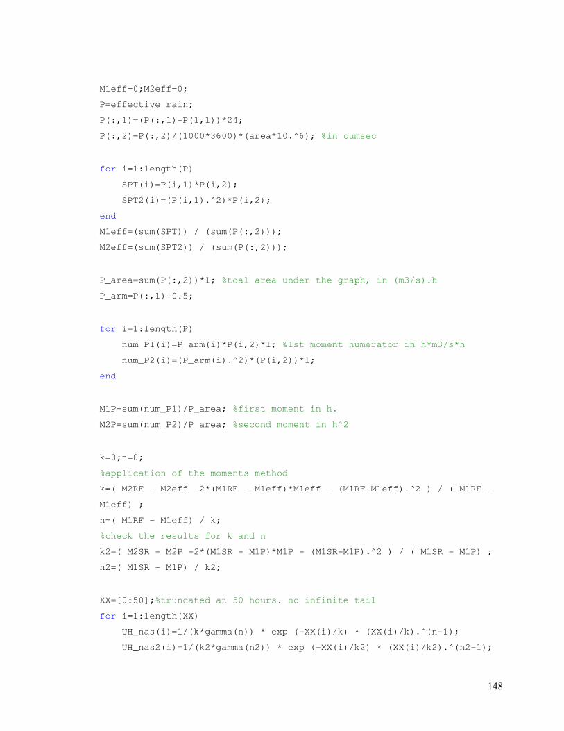
148
M1eff=0;M2eff=0;
P=effective_rain;
P(:,1)=(P(:,1)-P(1,1))*24;
P(:,2)=P(:,2)/(1000*3600)*(area*10.^6); %in cumsec
for i=1:length(P)
SPT(i)=P(i,1)*P(i,2);
SPT2(i)=(P(i,1).^2)*P(i,2);
end
M1eff=(sum(SPT)) / (sum(P(:,2)));
M2eff=(sum(SPT2)) / (sum(P(:,2)));
P_area=sum(P(:,2))*1; %toal area under the graph, in (m3/s).h
P_arm=P(:,1)+0.5;
for i=1:length(P)
num_P1(i)=P_arm(i)*P(i,2)*1; %1st moment numerator in h*m3/s*h
num_P2(i)=(P_arm(i).^2)*(P(i,2))*1;
end
M1P=sum(num_P1)/P_area; %first moment in h.
M2P=sum(num_P2)/P_area; %second moment in h^2
k=0;n=0;
%application of the moments method
k=( M2RF - M2eff -2*(M1RF - M1eff)*M1eff - (M1RF-M1eff).^2 ) / ( M1RF -
M1eff) ;
n=( M1RF - M1eff) / k;
%check the results for k and n
k2=( M2SR - M2P -2*(M1SR - M1P)*M1P - (M1SR-M1P).^2 ) / ( M1SR - M1P) ;
n2=( M1SR - M1P) / k2;
XX=[0:50];%truncated at 50 hours. no infinite tail
for i=1:length(XX)
UH_nas(i)=1/(k*gamma(n)) * exp (-XX(i)/k) * (XX(i)/k).^(n-1);
UH_nas2(i)=1/(k2*gamma(n2)) * exp (-XX(i)/k2) * (XX(i)/k2).^(n2-1);

149
end
UH_nas3=UH_nas*(area*10.^6)/(1000*3600);
%checking
for i=1:length(P(:,2))
for j=1:length(UH_nas)
Resp(j+i-1,i)=P(i,2)*UH_nas(j);
end
end
for i=1:length(Resp)
RESP(i)=sum(Resp(i,:));
end
RF_nas=RESP;
UH_nas=UH_nas3;
%-----GUHR -------------------------------------------------------
n=length(A); %number of reservoirs
GUHR=[];
for i=1:n
iA(i)=i*A(i);
end
K=sum(A)*(M1RF-M1eff)/sum(iA);
dt=1;
for t=1:50 % for t >dt
for i=1:n
for j=i:n
inter2(j)= 1/(gamma_paul(j-i))*( ((t-dt)/K).^(j-i)) *
sum(A(j:end) );
end
inter1(i)=1 / (gamma_paul(i-1)) * (t/K).^(i-1) *
sum(inter2(i:n));
inter3(i)=1 / (gamma_paul(i-1)) * (t/K).^(i-1) * sum(A(i:end));
end
GUHR(t)=1/dt*( exp(-(t-dt)/K)/sum(A)*sum(inter1) - exp(-
t/K)/sum(A)*sum(inter3) );
end
Resp_GUHR2=[];RESP_GUHR2=[];
for i=1:length(effective_rain)

150
for j=1:length(GUHR)
Resp_GUHR2(j+i-1,i)=effective_rain(i,2)*GUHR(j);
end
end
for i=1:length(Resp_GUHR2)
RESP_GUHR2(i)=sum(Resp_GUHR2(i,:));
end
UH_mor=GUHR;
RF_mor=RESP_GUHR2;

151
Appendix C
Matlab Code for the Unit Hydrograph Simulation
%[RF_nas,RF_ord,RF_mor]=SIM(stat,RF,effective_rain,A_ord,A_nas,A_mor)
%function SIM stands for simulation
%stat=duar/drom/kill
%RF=Response flow=direct runoff
%effective_rain=rainfall – losses
%A_ord,A_nas,A_mor are the respective UHs
%OUTPUT=Response Flows with OR ,Nash IUH and GUHR
function
[RF_nas,RF_ord,RF_mor]=SIM(stat,RF,effective_rain,A_ord,A_nas,A_mor)
%----------------------------------------------------------------------
%Unit hydrograph convolution : ORDINATES METHOD
X=[];UH=[];
UH=A_ord';
p=length(effective_rain); %p=number of rainfall imputs
n=length(UH);
m=n+p-1; %n=size oh the UH
X=zeros(m,n);
for j=1:n
for i=1:p
X(i+j-1,j)=effective_rain(i,2);
end
end
RF_ord=X*UH;
%-------------------Unit hydrograph convolution : NASH IUH METHOD
UH=[];X=[];UH=A_nas';
p=length(effective_rain); %p=number of rainfall imputs
n=length(UH);
m=n+p-1; %n=size oh the UH
X=zeros(m,n);
for j=1:n
for i=1:p
X(i+j-1,j)=effective_rain(i,2);

152
end
end
RF_nas=X*UH;
%----------------------Unit hydrograph convolution : GUHR METHOD
UH=[];X=[];UH=A_mor';
p=length(effective_rain); %p=number of rainfall imputs
n=length(UH);
m=n+p-1; %n=size oh the UH
X=zeros(m,n);
for j=1:n
for i=1:p
X(i+j-1,j)=effective_rain(i,2);
end
end
RF_mor=X*UH;
%------------------------plots the different simulation results
figure(222), plot(RF(:,2),'b'),hold on,
plot(RF_ord,'r')
plot(RF_nas,'g')
plot(RF_mor,'k')
legend('Observed','Odrinates','Nash IUH','GUHR')
hold off