NBER WORKING PAPER SERIES

RAILROADS OF THE RAJ:ESTIMATING THE IMPACT OF TRANSPORTATION INFRASTRUCTURE

Dave Donaldson

Working Paper 16487http://www.nber.org/papers/w16487

NATIONAL BUREAU OF ECONOMIC RESEARCH1050 Massachusetts Avenue

Cambridge, MA 02138October 2010

I am extremely grateful to Timothy Besley, Robin Burgess and Stephen Redding for their encouragementand support throughout this project. My thesis examiners, Richard Blundell and Chang-Tai Hsieh,and discussants, Costas Arkolakis and Samuel Kortum, provided detailed and valuable advice, andseminar audiences at Berkeley, BU, Brown, the CEPR (Development Economics Conference), Chicago,CIFAR, the Econometric Society European Winter Meetings, Harvard, the Harvard-Hitotsubashi-WarwickEconomic History Conference, IMF, LSE, MIT, Minneapolis Federal Reserve (Applied Micro Workshop),NBER Summer Institute (ITI), Northwestern, Nottingham, NYU, Oxford, Penn, Penn State, PhiladelphiaFederal Reserve, Princeton, Stanford, Toronto, Toulouse, UCL, UCLA, Warwick, Wharton, WorldBank, and Yale made thoughtful comments that improved this work. I am also grateful to ErasmusErmgassen, Rashmi Harimohan and Sritha Reddy for their help with the data; to the British Academy,the Nuffield Foundation, the Royal Economic Society, and STICERD for funding the data collection;and to the Bagri Fellowship and the DFID Program on Improving Institutions for Pro-Poor Growthfor financial support. The views expressed herein are those of the author and do not necessarily reflectthe views of the National Bureau of Economic Research.

NBER working papers are circulated for discussion and comment purposes. They have not been peer-reviewed or been subject to the review by the NBER Board of Directors that accompanies officialNBER publications.

© 2010 by Dave Donaldson. All rights reserved. Short sections of text, not to exceed two paragraphs,may be quoted without explicit permission provided that full credit, including © notice, is given tothe source.

Railroads of the Raj: Estimating the Impact of Transportation InfrastructureDave DonaldsonNBER Working Paper No. 16487October 2010JEL No. F15,N15,N75,O1,R13,R4

ABSTRACT

How large are the benefits of transportation infrastructure projects, and what explains these benefits?To shed new light on these questions, this paper uses archival data from colonial India to investigatethe impact of India's vast railroad network. Guided by four predictions from a general equilibriumtrade model, I find that railroads: (1) decreased trade costs and interregional price gaps; (2) increasedinterregional and international trade; (3) increased real income levels; and (4), that a sufficient statisticfor the effect of railroads on welfare in the model (an effect that is purely due to newly exploited gainsfrom trade) accounts for virtually all of the observed reduced-form impact of railroads on real incomein the data. I find no spurious effects from over 40,000 km of lines that were approved but - for fourdifferent reasons - were never built.

Dave DonaldsonMIT Department of Economics50 Memorial Drive, E52-243GCambridge, MA 02142-1347and NBERddonald@mit.edu

1 Introduction

In 2007, almost twenty percent of World Bank lending was allocated to transportation infras-

tructure projects, a larger share than that of education, health and social services combined

(World Bank, 2007). These projects aim to reduce the costs of trading. In prominent models

of international and interregional trade, reductions in trade costs will increase the level of real

income in trading regions. Unfortunately, despite an emphasis on reducing trade costs in both

economic theory and contemporary aid efforts, we lack a rigorous empirical understanding of

the extent to which transportation infrastructure projects actually reduce the costs of trading,

and how the resulting trade cost reductions affect welfare.

In this paper I exploit one of history’s great transportation infrastructure projects—the

vast network of railroads built in colonial India (India, Pakistan and Bangladesh; henceforth,

simply ‘India’)—to make three contributions to our understanding of transportation infras-

tructure improvements. In doing so I draw on a comprehensive new dataset on the colonial

Indian economy that I have constructed. First, I estimate the extent to which railroads im-

proved India’s trading environment (ie, reduced trade costs, reduced interregional price gaps,

and increased trade flows). Second, I estimate the reduced-form welfare gains (higher real

income levels) that the railroads brought about. Finally, I assess, in the context of a general

equilibrium trade model, how much of these reduced-form welfare gains could be plausibly

interpreted as newly exploited gains from trade.

The railroad network designed and built by the British government in India (then known to

many as ‘the Raj’) brought dramatic change to the technology of trading on the subcontinent.

Prior to the railroad age, bullocks carried most of India’s commodity trade on their backs,

traveling no more than 30 km per day along India’s sparse network of dirt roads (Deloche,

1994). By contrast, railroads could transport these same commodities 600 km in a day, and at

much lower per unit distance freight rates. As the 67,247 km long railroad network expanded

from 1853 to 1930, it penetrated inland districts (local administrative regions), bringing them

out of near-autarky and connecting them with the rest of India and the world. I use the

arrival of the railroad network in each district to investigate the economic impact of this

striking improvement in transportation infrastructure.

This setting is unique because the British government collected detailed records of eco-

nomic activity throughout India in this time period—remarkably, however, these records have

never been systematically digitized and organized by researchers. I use these records to con-

struct a new, district-level dataset on prices, output, daily rainfall and interregional and

international trade in India, as well as a digital map of India’s railroad network in which each

20 km segment is coded with its year of opening. This dataset allows me to track the evolution

of India’s district economies before, during, and after the expansion of the railroad network.

1

The availability of records on interregional trade is particularly unique and important here.

Information on trade flows within a country is rarely available to researchers, yet the response

of these trade flows to a transportation infrastructure improvement says a great deal about

the potential for gains from trade (as I describe explicitly below).

To guide my empirical analysis I develop a Ricardian trade model with many regions,

many commodities, and where trade occurs at a cost. Because of geographical heterogeneity,

regions have differing productivity levels across commodities, which creates incentives to trade

in order to exploit comparative advantage. A new railroad link between two districts lowers

their bilateral trade cost, allowing consumers to buy goods from the cheapest district, and

producers to sell more of what they are best at producing. There are thousands of interacting

product and factor markets in the model. But the analysis of this complex general equilibrium

problem is tractable if production heterogeneity takes a convenient but plausible functional

form, as shown by Eaton and Kortum (2002).

I use this model to assess empirically the importance of one particular mechanism linking

railroads to welfare improvements—that railroads reduced trade costs and thereby allowed

regions to gain from trade. The model makes four predictions that drive my four-step empirical

analysis:

1. Inter-district price differences are equal to trade costs (in special cases): That is, if a

commodity can be made in only one district (the ‘origin’) but is consumed in other

districts, then that commodity’s origin-destination price difference is equal to its origin-

destination trade cost. Empirically, I use this result to measure trade costs (which, like

all researchers, I cannot observe directly) by exploiting widely-traded commodities that

could only be made in one district. Using inter-district price differentials, along with a

graph theory algorithm embedded in a non-linear least squares routine, I estimate the

trade cost parameters governing traders’ endogenous route decisions on a network of

roads, rivers, coasts and railroads. This is a novel method for inferring trade costs in

networked settings. My resulting parameter estimates reveal that railroads significantly

reduced the cost of trading in India.

2. Bilateral trade flows take the ‘gravity equation’ form: That is, holding constant exporter-

and importer-specific effects, bilateral trade costs reduce bilateral trade flows. Empir-

ically, I use the estimate from a gravity equation, in conjunction with the trade cost

parameters estimated in Step 1, to identify all of the relevant unknown parameters of

the model.

3. Railroads increase real income levels: That is, when a district is connected to the railroad

network its real income rises. Empirically, I find that railroad access raises real income

2

by 16 percent. This reduced-form estimate could arise through a number of economic

mechanisms. A key goal of Step 4 below is to assess how much of the reduced-form

impact of railroads on real income can be attributed to gains from trade due to the

trade cost reductions found in Step 1.

4. There exists a sufficient statistic for the welfare gains from railroads: That is, despite the

complexity of the model’s general equilibrium relationships, the impact of the railroad

network on welfare in a district is captured by its impact on one endogenous variable:

the share of that district’s expenditure that it sources from itself. A prediction similar to

this appears in a wide range of trade models but has not, to my knowledge, been tested

before.1 Empirically, I test this prediction by regressing real income on this sufficient

statistic (as calculated using the model’s parameter estimates obtained in Steps 1 and

2) alongside the regressors from Step 3 (which capture the reduced-form impact of

railroads). When I do this, the estimated reduced-form coefficients on railroad access

(from Step 3) fall to a level that is close to zero. This finding provides support for

Prediction 4 of the model and implies that decreased trade costs account for virtually

all of the real income impacts of the Indian railroad network.

These four results demonstrate that India’s railroad network improved the trading envi-

ronment (Steps 1 and 2) and generated welfare gains (Steps 3), and suggest that these welfare

gains arose predominantly because railroads allowed regions to exploit gains from trade (Step

4).

A natural concern when estimating the impact of infrastructure projects is that of bias

due to a potential correlation between project placement and unobserved changes in the local

economic environment. These concerns are likely to be less important in my setting because

(as described in Section 2) military motives for railroad placement usually trumped economic

arguments, the networked nature of railroad technology inhibited the ability of planners to

target specific locations precisely, and planning documents reveal just how hard it was for

technocrats to agree on the efficacy of railroad plans. Nevertheless, to mitigate concerns of

selection bias I estimate the ‘effects’ of over 40,000 km of railroad lines that reached advanced

stages of costly surveying but—for four separate reasons that I document in Section 6—were

never actually built. Reassuringly, these ‘placebo’ lines never display spurious effects.

This paper contributes to a growing literature on estimating the economic effects of large

infrastructure projects,2 as well as to a literature on estimating the ‘social savings’ of rail-

1Arkolakis, Costinot, and Rodriguez-Clare (2010) show that this prediction applies to the Krugman (1980),Eaton and Kortum (2002), and Chaney (2008) models of trade, but these authors do not test this predictionempirically.

2For example, Dinkelman (2007) estimates the effect of electrification on labor force participation in South

3

road projects.3 A distinguishing feature of my approach is that, in addition to estimating

reduced-form relationships between infrastructure and welfare, as in the existing literature, I

fully specify and estimate a general equilibrium model of how railroads affect welfare.4 The

model makes auxiliary predictions and suggests a sufficient statistic for the role played by

railroads in raising welfare—all of which shed light on the economic mechanisms that could

explain my reduced-form estimates. Using a model also improves the external validity of my

estimates because the primitive in my model—the cost of trading—is specified explicitly, and

is portable to a range of settings (such as tariff liberalization or road construction) in which the

welfare benefits of trade cost-reducing polices might be sought. By contrast, my reduced-form

estimates are more likely to be specific to the context of railroads in colonial India.

This paper also contributes to a rich literature concerned with estimating the welfare

effects of openness to trade, because the reduction in trade costs brought about by India’s

railroad network rapidly increased each district’s opportunities to trade.5 Again, the fact that

my empirical approach connects explicitly to an estimable, general equilibrium model of trade

offers advantages over the existing literature. The model suggests a theoretically-consistent

way to measure ‘openness,’ sheds light on why trade openness raises welfare, and provides a

natural way to study changes in openness to both internal and external trade at the same

time.

The next section describes the historical setting in which the Indian railroad network was

constructed and the new data that I have collected from that setting. In Section 3, I outline a

model of trade in colonial India and the model’s four predictions. Sections 4 through 7 present

four empirical steps that test the model’s four predictions qualitatively and quantitatively.

Section 8 concludes.

Africa, Duflo and Pande (2007) estimate the effect of dam construction in India on agriculture, Jensen (2007)evaluates how the construction of cellular phone towers in South India improved efficiency in fish markets,and Michaels (2008) estimates the effect of the US Interstate Highway system on the skilled wage premium.An older literature, beginning with Aschauer (1989), pioneered the use of econometric methods in estimatingthe benefits of infrastructure projects.

3Fogel (1964) first applied the social savings methodology to railroads in the United States, and Hurd(1983) performed a similar exercise for India. In Section 6.5 I compare my estimates to those from using asocial savings approach.

4The use of general equilibrium modeling, on its own, to evaluate transportation projects here is not novel.For example, both Williamson (1974) and Herrendorf, Schmitz, and Teixeira (2009) use calibrated generalequilibrium models to study the impact of railroads on the antebellum US economy.

5Frankel and Romer (1999), Alcala and Ciccone (2004), Feyrer (2009) and others use cross-country regres-sions of real GDP levels on ‘openness’ (defined in various ways) to estimate the effect of openness on welfare.Pavcnik (2002), Trefler (2004), and Topalova (forthcoming) among others instead analyze trade liberalizationswithin one country by exploiting cross-sectional variation in the extent of liberalization across either industriesor regions.

4

2 Historical Background and Data

In this section I discuss some essential features of the colonial Indian economy and the data

that I have collected in order to analyze how this economy changed with the advent of railroad

transport. I go on to describe the transportation system in India before and after the railroad

era, and the institutional details that determined when and where railroads were built.

2.1 New Data on the Indian Economy, 1870-1930

In order to evaluate the impact of the railroad network on economic welfare in colonial India

I have constructed a new panel dataset on 235 Indian districts. The dataset tracks these

districts annually from 1870-1930, a period during which 98 percent of British India’s current

railroad lines were opened. Table 1 contains descriptive statistics for the variables that I use

in this paper and describe throughout this section. Appendix A contains more detail on the

construction of these variables.

During the colonial period, India’s economy was predominantly agricultural, with agricul-

ture constituting an estimated 66 percent of GDP in 1900 (Heston, 1983).6 For this reason,

district-level output data were only collected systematically in the agricultural sector. Data on

agricultural output were recorded for each of 17 principal crops (which comprised 93 percent

of the cropped area of India in 1900).7 Retail prices for these 17 crops were also recorded at

the district-level. I use these price figures to construct a nominal agricultural output series

for each district and year and then a real agricultural income per acre figure by dividing nom-

inal output by a consumer price index and district land area. The resulting real agricultural

income per acre variable provides the best available measure of district-level economic welfare

in this time period.

Real incomes were low during my sample period, but there was 22 percent growth between

1870 and 1930.8 Real incomes were low because crop yields were low, both by contemporaneous

international standards and by Indian standards today.9 One explanation for low yields, which

featured heavily in Indian agricultural textbooks of the day (such as Wallace (1892)), was

6Factory-based industry—which Atack, Haines, and Margo (forthcoming) argue benefited from access torailroads in the United States—amounted to only 1.6 percent of India’s GDP in 1900.

7These crops are: bajra, barley, bengal gram, cotton, indigo, jowar, kangni, linseed, maize, opium, ragi,rape and mustard seed, rice, sesamum, sugarcane, tur and wheat.

8For comparison, Heston (1983) estimates that in 1869, on the basis of purchasing power exchange rates,per capita income in the United States was four times that in India. This income disparity rises to ten ifmarket exchange rates are used instead of PPP rates.

9For example, the yield of wheat in India’s ‘breadbasket’, the province of Punjab, was 748 lbs/acre in 1896.By contrast, for similar types of wheat, yields in Nevada (the highest state yields in the United States) in1900 were almost twice as high (see plate 15 of United States Census Office (1902)) and yields in (Indian)Punjab in 2005 were over five times higher than those in 1896 (as calculated from the Indian District-wiseCrop Production Statistics Portal, http://dacnet.nic.in/apy/cps.aspx).

5

inadequate water supply. Only 12 percent of cultivated land was irrigated in 1885 and while

this figure had risen to 19 percent in 1930, the vast majority of agriculture maintained its

dependence on rainfall.10

Because rainfall was important for agricultural production, 3614 meteorological stations

were built throughout the country to record the amount of rainfall at each station on every

day of the year. Daily rainfall data were recorded and published because the distribution

of rainfall throughout the year was far more important to farmers and traders than total

annual or monthly amounts. In particular, the intra-annual distribution of rainfall governed

how different crops (which were grown in distinct stretches of the year) were affected by a

given year’s rainfall. In Sections 5 and 7 below, I use daily rainfall data collected from India’s

meteorological stations to construct crop-specific measures of rainfall and use these as a source

of exogenous variation in crop-specific productivity.

Commensurate with the increase in real agricultural income levels in India was a significant

rise in interregional trade. The final component of the dataset that I have constructed on

colonial India consists of data on these internal trades whenever they occurred via railroad,

river or sea (data on road trade was only very rarely collected). The role that these data play

in my analysis is explained in Section 5 below.

2.2 Transportation in Colonial India

Prior to the railroad era, goods transport within India took place on roads, rivers, and coastal

shipping routes.11 The bulk of inland travel was carried by bullocks, along the road network.

On the best road surfaces and during optimal weather conditions, bullocks could pull a cart

of goods and cover 20-30 km per day. However, high-quality roads were extremely sparse and

the roads that did exist were virtually impassable in the monsoon season. For this reason

most trade was carried by ‘pack’ bullocks (which carried goods strapped to their backs and

usually traveled directly over pasture land), which were considerably slower and riskier than

cart bullocks.

Water transport was far superior to road transport, but it was only feasible on the Brahma-

putra, Ganges and Indus river systems.12 In optimal conditions, downstream river traffic (with

additional oar power13) could cover 65 km per day; upstream traffic needed to be towed from

10These figures encompass a wide definition of irrigation, including the use of tanks, cisterns, and reservoirsas well as canals. See the Agricultural Statistics of India, described in Appendix A. 1885 is the first year inwhich comprehensive irrigation statistics were collected.

11The description of pre-rail transportation in this section draws heavily on the comprehensive treatmentsof Deloche (1994), Deloche (1995), and Derbyshire (1985).

12Navigable canals either ran parallel to sections of these three rivers or were extremely localized in a smallnumber of coastal deltas (Stone, 1984).

13Steamboats had periods of success in the colonial era, but were severely limited in scope by India’s seasonal

6

the banks and struggled to cover 15 km per day. Extensive river travel was impossible in the

rainy monsoon months or the dry summer months and piracy was a serious hazard. Coastal

shipping, however, was perennially available along India’s long coastline. This form of ship-

ping was increasingly steam-powered after 1840. Steamships were fast and could cover over

100 km per day but could only service major ports (Naidu, 1936).

Against this backdrop of costly and slow internal transportation, the appealing prospect

of railroad transportation in India was discussed as early as 1832 (Sanyal, 1930)—though it

was not until 1853 that the first track was actually laid. From the outset, railroad transport

proved to be far superior to road, river or coastal transport (Banerjee, 1966). Trains were

capable of traveling up to 600 km per day and they offered this superior speed on predictable

timetables, throughout all months of the year, and without any serious threat of piracy or

damage (Johnson, 1963). Railroad freight rates were also considerably cheaper: 4-5, 2-4, and

1.5-3 times cheaper than road, river and coastal transport, respectively. A principal goal of

Section 4 below is to estimate how much railroad technology reduced total trade costs, costs

which combine all of these attractions of railroads over other modes.

2.3 Railroad Line Placement Decisions

Throughout the history of India’s railroads, all railroad line placement decisions were made

by the Government of India. It is widely accepted that the Government had three mo-

tives for building railroads: military, commercial, and humanitarian—in that order of priority

(Thorner, 1950; Macpherson, 1955; Headrick, 1988). In 1853, Lord Dalhousie (head of the

Government of India) wrote an internal document to the East India Company’s Court of

Directors that made the case for a vast railroad network in India and military motives for

railroad-building appeared on virtually every page of this document14. These arguments gath-

ered new momentum when the 1857 ‘mutiny’ highlighted the importance of military commu-

nications (Headrick, 1988). Dalhousie’s 1853 minute described five “trunk lines” that would

connect India’s five major provincial capitals along direct routes and maximize the “political

advantages” of a railroad network.

Between 1853 and 1869, all of Dalhousie’s trunk lines were built—but not without signifi-

cant debate over how best to connect the provincial capitals. Dalhousie and Major Kennedy,

India’s Chief Engineer, spent over a decade discussing and surveying their competing—and

and shifting rivers.14For example, from the introduction: “A single glance...will suffice to show how immeasurable are the

political advantages to be derived from the system of internal communication, which would admit of fullintelligence of every event being transmitted to the Government...and would enable the Government to bringthe main bulk of its military strength to bear upon any given point in as many days as it would now requiremonths, and to an extent which at present is physically impossible.” (House of Commons Papers, 1853).

7

very different—proposals for a pan-Indian network (Davidson, 1868; Settar, 1999). This de-

bate indicates the vicissitudes of railroad planning in India and it was repeated many times

by different actors in Indian railroad history. I have collected planning documents from a

number of railroad expansion proposals that, along with Kennedy’s proposal, were debated

and surveyed at length, but were never actually built. As discussed in Section 6.4 below, I

use these plans in a ‘placebo’ strategy to check that unbuilt lines display no spurious ‘impact’

on the district economies in which they were nearly built.

As is clear from Figure 1, the railroad network in place in 1930 (by and large, the same

network that is open today) had completely transformed the transportation system in India.

67,247 km of track were open for traffic, constituting the fourth-largest network in the world.

From their inception in 1853 to their zenith in 1930, railroads were the dominant form of

public investment in British India. But influential observers were highly critical of this public

investment priority—the Nationalist historian, Romesh Dutt, argued that they did little to

promote agricultural development,15 and Mahatma Gandhi argued simply that, “there can be

little doubt that [railroads] promote evil” (Gandhi, 1938). In the remainder of this paper I

use new data to assess quantitatively the effect of railroads on India’s trading environment

and agricultural economy.

3 A Model of Railroads and Trade in Colonial India

In this section I develop a general equilibrium model of trade among many regions in the

presence of trade costs. The model is based on Eaton and Kortum (2002), but with more

than one commodity, and serves two purposes. First, it delivers four predictions about the

response of observables to trade cost reductions. Second, I estimate the unknown parameters

of the model and use the estimated model to assess whether the observed reduction in trade

costs due to the railroads can account, via the mechanism stressed in this model, for the

observed increase in welfare due to railroads. Both of these features inform our understanding

of how transportation infrastructure projects can raise welfare.

3.1 Model Environment

The economy consists of D regions (indexed by either o or d). There are K commodities

(indexed by k), each available in a continuum (with mass normalized to one) of horizontally

differentiated varieties (indexed by j). In my empirical application I work with data on prices,

15For example, on page 174 of his landmark textbook on Indian economic history: “Railways...did not addto the produce of the land.” (Dutt, 1904)

8

output and trade flows that refer to commodities, not individual varieties. While my empir-

ical setting will consider 70 years of annual observations, for simplicity the model is static; I

therefore suppress time subscripts until they are necessary.

Consumer Preferences:

Each region o is home to a mass (normalized to one) of identical agents, each of whom owns Lo

units of land. Land is geographically immobile and supplied inelastically. Agents have Cobb-

Douglas preferences over commodities (k) and constant elasticity of substitution preferences

over varieties (j) within each commodity; that is, their (log) utility function is

lnUo =K∑k=1

(µkεk

)ln

∫ 1

0

(Cko (j))εkdj, (1)

where Cko (j) is consumption, εk

.= σk−1

σk(where σk is the constant elasticity of substitution),

and∑

k µk = 1. Agents rent out their land at the rate of ro per unit and use their income

roLo to maximize utility from consumption.

Production and Market Structure:

Each variety j of the commodity k can be produced using a constant returns to scale produc-

tion technology in which land is the only factor of production. Let zko (j) denote the amount

of variety j of commodity k that can be produced with one unit of land in region o. I follow

Eaton and Kortum (2002) in modeling zko (j) as the realization of a stochastic variable Zko

drawn from a Type-II extreme value distribution whose parameters vary across regions and

commodities in the following manner

F ko (z)

.= Pr(Zk

o ≤ z) = exp(−Akoz−θk), (2)

where Ako ≥ 0 and θk > 0. These random variables are drawn independently for each variety,

commodity and region.16 The exogenous parameter Ako increases the probability of high

productivity draws and the exogenous parameter θk captures (inversely) how variable the

(log) productivity of commodity k in any region is around its (log) average.

There are many competitive firms in region o with access to the above technology; conse-

quently, firms make zero profits.17 These firms will therefore charge a pre-trade costs (ie, ‘free

16Costinot, Donaldson, and Komunjer (2010) show that the key features of the Eaton and Kortum (2002)model hold locally around a symmetric distribution of exogenous productivity terms Ako for any continuousproductivity distribution.

17My empirical application is primarily to the agricultural sector. This sector was characterized by millionsof small-holding farmers who were likely to be price-taking producers of undifferentiated products (varieties jin the model). For example, in the 1901 census in the province of Madras, workers in the agricultural sector

9

on board’) price of pkoo(j) = ro/zko (j), where ro is the land rental rate in region o.

Opportunities to Trade:

Without opportunities to trade, consumers in region d must consume even their region’s worst

draws from the productivity distribution in equation (2). The ability to trade breaks this

production-consumption link. This allows consumers to import varieties from other regions

in order to take advantage of the favorable productivity draws available there, and allows

producers to produce more of the varieties for which they received the best productivity

draws. These two mechanisms constitute the gains from trade in this model.

However, there is a limit to trade because the movement of goods is subject to trade

costs (which include transport costs and other barriers to trade). These trade costs take the

convenient and commonly used ‘iceberg’ form. That is, in order for one unit of commodity

k to arrive in region d, T kod ≥ 1 units of the commodity must be produced and shipped in

region o; trade is free when T kod = 1. (Throughout this paper I refer to trade flows between

an origin region o and a destination region d; all bilateral variables, such as T kod, refer to

quantities from o to d.) Trade costs are assumed to satisfy the property that it is always

(weakly) cheaper to ship directly from region o to region d, rather than via some third region

m: that is, T kod ≤ T komTkmd. Finally, I normalize T koo = 1. In my empirical setting I proxy for T kod

with measures calculated from the observed transportation network, which incorporates all

possible modes of transport between region o and region d. Railroads enter this transportation

network gradually over time, reducing T kod and creating more gains from trade.

Trade costs drive a wedge between the price of an identical variety in two different re-

gions. Let pkod(j) denote the price of variety j of commodity k produced in region o, but

shipped to region d for consumption there. The iceberg formulation of trade costs implies

that any variety in region d will cost T kod times more than it does in region o; that is,

pkod(j) = T kod pkoo(j) = ro T

kod/z

ko (j).

Equilibrium Prices and Allocations:

Consumers have preferences for all varieties j along the continuum of varieties of commodity

k. But they are are indifferent about where a given variety is made—they simply buy from

the region that can provide the variety at the lowest cost (after accounting for trade costs).

I therefore solve for the equilibrium prices that consumers in a region d actually pay, given

that they will only buy a given variety from the cheapest source region (including their own).

The price of a variety sent from region o to region d, denoted by pkod(j), is stochastic

(67.9 percent of the almost 20 million strong workforce) were separately enumerated by their ownership status,and 35.7 percent of these workers were owner-cultivators, or proprietors of extremely small-scale farms (Risleyand Gait, 1903).

10

because it depends on the stochastic variable zko (j). Since zko (j) is drawn from the CDF in

equation (2), pkod(j) is the realization of a random variable P kod drawn from the CDF

Gkod(p)

.= Pr(P k

od ≤ p) = 1 − exp[−Ako(roT kod)−θkpθk ]. (3)

This is the price distribution for varieties (of commodity k) made in region o that could

potentially be bought in region d. The price distribution for the varieties that consumers in d

will actually consume (whose CDF is denoted by Gkd(p)) is the distribution of prices that are

the lowest among all D regions of the world:

Gkd(p) = 1 −

D∏o=1

[1 −Gkod(p)],

= 1 − exp

(−

[D∑o=1

Ako(roTkod)

−θk

]pθk

).

Given this distribution of the actual prices paid by consumers in region d, it is straight-

forward to calculate any moment of the prices of interest. The price moment that is relevant

for my empirical analysis is the expected value of the equilibrium price of any variety j of

commodity k found in region d, which is given by

E[pkd(j)].= pkd = λk1

[D∑o=1

Ako(roTkod)

−θk

]−1/θk

, (4)

where λk1.= Γ(1 + 1

θk).18 In my empirical application below I treat these expected prices as

equal to the observed prices collected by statistical agencies.19

Given the price distribution in equation (3), Eaton and Kortum (2002) derive two im-

portant properties of the trading equilibrium that carry over to the model here. First, the

price distribution of the varieties that any given origin actually sends to destination d (ie,

the distribution of prices for which this origin is region d’s cheapest supplier) is the same

for all origin regions. This implies that the share of expenditure that consumers in region d

allocate to varieties from region o must be equal to the probability that region o supplies a

18Γ(.) is the Gamma function defined by Γ(z) =∫∞0tz−1e−tdt.

19 A second price moment that is of interest for welfare analysis is the exact price index over all varieties

of commodity k for consumers in region d. Given CES preferences, this is pkd.=[∫ 1

0(pkd(j))1−σkdj

]1/1−σk

,

which is only well defined here for σk < 1 + θk (a condition I assume throughout). The exact price index is

given by pkd = λk2pkd, where λk2

.= γk

λk1

and γk.= [Γ( θk+1−σk

θk)]1/(1−σk). That is, if statistical agencies sampled

varieties in proportion to their weights in the exact price index, as opposed to randomly as in the expectedprice formulation of equation (4), then this would not jeopardize my empirical procedure because the exactprice index is proportional to expected prices.

11

variety to region d (because the price per variety, conditional on the variety being supplied to

d, does not depend on the origin). That is Xkod/X

kd = πkod, where Xk

od is total expenditure in

region d on commodities of type k from region o, Xkd.=∑

oXkod is total expenditure in region

d on commodities of type k, and πkod is the probability that region d sources any variety of

commodity k from region o. Second, this probability πkod is given by

Xkod

Xkd

= πkod = λk3 Ako (roT

kod)

−θk (pkd)θk , (5)

where λk3 = (λk1)−θk , and this equation makes use of the definition of the expected value of

prices (ie, pkd) from equation (4).

Equation (5) characterizes trade flows conditional on the endogenous land rental rate, ro

(and all other regions’ land rental rates, which appear in pkd). It remains to solve for these land

rents in equilibrium, by imposing the condition that each region’s trade is balanced. Region

o’s trade balance equation requires that the total income received by land owners in region o

(roLo) must equal the total value of all commodities made in region o and sent to every other

region (including region o itself). That is:

roLo =∑d

∑k

Xkod =

∑d

∑k

πkod µk rd Ld, (6)

where the last equality uses the fact that (with Cobb-Douglas preferences) expenditure in

region d on commodity k (Xkd ) will be a fixed share µk of the total income in region d (ie,

of rdLd). Each of the D regions has its own trade balance equation of this form. I take the

rental rate in the first region (r1) as the numeraire good, so the equilibrium of the model is

the set of D-1 unknown rental rates rd that solves this system of D-1 (non-linear) independent

equations.

3.2 Four Predictions

In this section I state explicitly four of the model’s predictions. These predictions are pre-

sented in the order in which they drive my empirical analysis (ie, Steps 1-4) below.

Prediction 1: Price differences measure trade costs (in special cases):

In the presence of trade costs, the price of identical commodities will differ across regions. In

general, the cost of trading a commodity between two regions places only an upper bound on

their price differential. However, in the special case of a homogeneous commodity that can

only be produced in one origin region, equation (4) predicts that the (log) price differential

between the origin o of this commodity and any other region d will be equal to the (log) cost

12

of trading the commodity between them. That is:

ln pod − ln poo = lnT ood, (7)

where the commodity label k is replaced by o to indicate that this equation is only true for

commodities that can only be made in region o. This prediction is important for my empirical

work below because it allows trade costs (T ood), which are never completely observed, to be

inferred. But it is important to note that this prediction—essentially just free arbitrage over

space, net of trade costs—is common to many models of spatial equilibrium.20

Prediction 2: Bilateral trade flows take the ‘gravity equation’ form:

Equation (5) describes bilateral trade flows explicitly, but I re-state it here in logarithms for

reference: (log) bilateral trade of any commodity k from any region o to any other region d is

given by

lnXkod = lnλk + lnAko − θk ln ro − θk lnT kod + θk ln pkd + lnXk

d . (8)

This is the gravity equation form for bilateral trade flows, which is common to many widely-

used trade models: bilateral trade costs reduce bilateral trade flows, conditional on importer-

and exporter-specific terms.

Prediction 3: Railroads increase real income levels:

In this model, welfare in district o is equal to its real income (per unit land area), Wo, which

is given by real land rents:21

Wo =ro∏K

k=1(pko)µk

.=ro

Po. (9)

Unfortunately, the multiple general equilibrium interactions in the model are too complex to

admit a closed-form solution for the effect of reduced trade costs on welfare. To make progress

in generating qualitative predictions (to guide my empirical analysis) I therefore assume a

much simpler environment for the purpose of obtaining Prediction 3 only. I assume: there are

only three regions (called X, Y and Z); there is only one commodity (so I will dispense with the

k superscripts on all variables); the regions are symmetric in their exogenous characteristics

(ie, Lo and Ao); and the three regions have symmetric trade costs with respect to each other.

20A class of exceptions is those with some form of imperfect competition and in which producers cancharge separate prices in separate markets, as in Brander and Krugman (1983) or Melitz and Ottaviano(2007). However, my empirical application of this prediction will be to salt, which was produced under strictgovernment license at a small number of locations and then had to be sold (under conditions of the license) toan unrestricted trading community at the ‘factory’ gate (United Provinces of Agra and Oudh, 1868). That is,in this setting, producers only charged one factory gate price and could not price discriminate across markets.

21Recall that pko is the CES price index for commodity k in region o, defined in footnote 19.

13

I consider the comparative statics from a local change around this symmetric equilibrium

that reduces the bilateral trade cost symmetrically between two regions (say X and Y ). It is

straightforward to show (as is done in Appendix B) that:

dWX

dTY X< 0. (10)

That is, real income in a region (say, X) rises when the bilateral cost of trading between that

region and any other region (say, Y ) falls.

Prediction 4: There exists a sufficient statistic for the welfare gains from railroads:

Using the bilateral trade equation (5) evaluated at d = o, (log) real income per unit of land

can be re-written as

lnWo = Ω +∑k

µkθk

lnAko −∑k

µkθk

ln πkoo, (11)

where Ω.= −

∑k µk ln γk. This result states that welfare is a function of only two terms,

one involving (exogenous) local productivity levels (Ako), and a second term that I will refer

to as ‘autarkiness’ (ie, the fraction of region o’s expenditure that region o buys from itself,

πkoo, which equals one in autarky). Because of the complex general equilibrium relationships

in the model, the full matrix of trade costs (between every bilateral pair of regions), the full

vector of productivity terms in all regions, and the sizes of all regions all influence welfare

in region o. But these terms (that is, every exogenous variable in the model other than

local productivity) affect welfare only through their effect on autarkiness. Put another way,

autarkiness (the appropriately weighted sum of πkoo terms over goods k) is a sufficient statistic

for welfare in region o, once local productivity is controlled for. If railroads affected welfare

in India through the mechanism in the model (by reducing trade costs, giving rise to gains

from trade), then Prediction 4 states that one should see no additional effects of railroads on

welfare once autarkiness (πkoo) is controlled for.

3.3 From Theory to Empirics

To relate the static model in Section 3 to my dynamic empirical setting (with 70 years of annual

data) I take the simplest possible approach and assume that all of the goods in the model

cannot be stored, and that inter-regional lending is not possible. Furthermore, I assume that

the stochastic production process described in Section 3.1 is drawn independently in each

period. These assumptions imply that the static model simply repeats every period, with

independence of all decision-making across time periods. Throughout the remainder of the

paper I therefore add the subscript ‘t’ to all of the variables (both exogenous and endogenous)

14

in the model, but I assume that all of the model parameters θk, σk, and µk are fixed over time.

The four theoretical predictions outlined in Section 3.2 take a naturally recursive order,

both for estimating the model’s parameters, and for tracing through the impact of railroads

on welfare in India. I follow this order in the four empirical sections that follow below (ie,

Steps 1-4). In Step 1, I evaluate the extent to which railroads reduced trade costs within India

using Prediction 1 to relate the unobserved trade costs term in the model (T kodt) to observed

features of the transportation network. In Step 2, I use Prediction 2 to measure how much

the reduced trade costs found in Step 1 increased trade in India. This relationship allows

me to estimate the unobserved model parameter θk (the elasticity of trade flows with respect

to trade costs), and to relate the unobserved productivity terms (Akot)22 to rainfall, which is

an exogenous and observed determinant of agricultural productivity. Steps 1 and 2 therefore

deliver estimates of all of the model’s parameters.

In Step 3, I test Prediction 3 by estimating how the level of a district’s real income is

affected by the arrival of railroad access to the district. However, the empirical finding in Step

3 is reduced-form in nature and could arise through a number of possible mechanisms (such

as enhanced mobility labor, capital or technology). Therefore, in Step 4 I use the sufficient

statistic suggested by Prediction 4 to compare the reduced-form effects of railroads on the

level of real income (found in Step 3) with the effects predicted by the model (as estimated

in Steps 1 and 2).

4 Empirical Step 1: Railroads and Trade Costs

In the first step of my empirical analysis I estimate the extent to which railroads reduced the

cost of trading within India. Because this paper explores a trade-based mechanism for the

impact of railroads on welfare, it is important to assess whether railroads actually reduced

trade costs. Further, the relationship between railroads and trade costs, which I estimate in

this section, is an important input for Steps 2 and 4 that follow.

4.1 Empirical Strategy

Researchers never observe the full extent of trade costs.23 But Prediction 1 suggests a situation

in which trade costs can be inferred : If a homogeneous commodity can only be made in one

22The productivity terms Akot are unobserved because they represent the location parameter on region o’spotential productivity distribution of commodity k, in equation (2). The productivities actually used forproduction in region o will be a subset of this potential distribution, where the scope for trade endogenouslydetermines how the potential distribution differs from the distribution actually used to produce.

23Even when shipping receipts are observed, as in Hummels (2007), these may fail to capture other barriersto trade, such as the time goods spend in transit, or the risk of damage or loss in transit.

15

region, then the difference in retail prices (of that commodity) between the origin region and

any other consuming region is equal to the cost of trading between the two regions.24

Throughout Northern India, several homogeneous types of salt were consumed, but each

of these types could only be made in one unique location. Traders and consumers would speak

about ‘Kohat salt’ (which could only be produced at the salt mine in the Kohat region) as a

different commodity from ‘Sambhar salt’ (which could only be produced at the Sambhar Salt

Lake).25 I have collected data on salt prices in Northern India, in which the prices of eight

regionally-differentiated types of salt are reported in 124 districts annually from 1861-1930.

Crucially, because salt is an essential commodity, it was consumed (and therefore sold at

markets where its price could be easily recorded) throughout India both before and after the

construction of railroads.

I use these salt price data, with the help of Prediction 1, to estimate how Indian railroads

reduced trade costs. To do this I estimate equation (7) of Prediction 1 as follows:

ln podt = βoot︸︷︷︸=ln poot

+ βood + δ lnLCRED(Rt,α)odt + εoodt︸ ︷︷ ︸=lnT o

odt

. (12)

In this equation, podt is the price of type-o salt (that is, salt that can only be made in region

o) in destination district d in year t. I estimate this equation with an origin-year fixed effect26

(βoot) to control for the price of type-o salt at its origin o (ie, poot) because I do not observe

salt prices exactly at the point where they leave the source. (My price data are at the district

level and are based on records of the price of a commodity averaged over 10-15 retail markets

in a district.)

The remainder of equation (12) describes how I model the relationship between trade costs

T oodt, which are unobservable, and the railroad network (denoted by Rt), which is observable.

The core of this specification is the variable LCRED(Rt,α), which I describe in detail below.

This specification also includes an origin-destination fixed effect (βood) which controls for all

of the time-invariant determinants of the cost of trading salt between districts o and d (such

24In their survey of attempts to estimate trade costs, Anderson and van Wincoop (2004) suggest (on p. 78)the solution I pursue here: “A natural strategy would be to identify the source [region] for each product. We arenot aware of any papers that have attempted to measure trade barriers this way.” Recent work by Keller andShiue (2008) on 19th Century Germany and Andrabi and Kuehlwein (2010) on colonial India documents thatwhen two markets are connected by railroad lines, these markets’ prices (for similar commodities) converge.This approach demonstrates that railroads lowered trade costs, but does not aim to estimate the level of tradecosts or the magnitude of the effect of railroads on trade costs.

25The leading (nine-volume) commercial dictionary in colonial India, Watt (1889), describes the market forsalt in this manner, as do Aggarwal (1937) and the numerous provincial Salt Reports that were brought outeach year.

26That is, each salt origin o has its own fixed effect in each year t. I use this notation when referring tofixed effects throughout this paper.

16

as the distance from o to d, or caste-based or ethno-linguistic differences between o and d

that may hinder trade). Finally, εoodt is an error term that captures any remaining unobserved

determinants of trade costs (or measurement error in ln podt).27

The variable LCRED(Rt,α) in equation (12) measures the lowest-cost route effective

distance between the origin o and destination d districts in any year t. This variable models

the cost of trading goods between any two locations under the assumption that agents take

the lowest-cost route—using any mode of transportation—available to them. Two inputs are

needed to calculate the effective length of the lowest-cost route between districts o and d

in year t. The first input is the network of available transportation routes open in year t,

which I denote by Rt. A network is a collection of nodes and arcs. In my application, nodes

are finely-spaced points in space, and arcs are available means of transportation between the

nodes (hence an arc could be a rail, river, road or coast connection). In modeling this network

(detailed in Appendix A) I allow agents to travel on navigable rivers, the coastline, the road

network, and the railroad network open in year t.

The second input is the cost of traveling along each arc, which depends on which mode

of transportation the arc represents. I model these costs as being proportional to distance,

where the proportionality, the per unit distance cost, of using each mode is denoted by the

vector of parameters α.= (αrail, αroad, αriver, αcoast). I normalize αrail = 1 so the other three

elements of α represent costs relative to the cost of using railroads. Because of this nor-

malization, LCRED(Rt,α)odt is measured in units of railroad-equivalent kilometers; in this

sense, a finding that all of the non-rail elements of α are greater than one would imply

that India’s expanding railroad network shrunk ‘effective distance,’ or distance measured in

railroad-equivalent units.

The parameter α is unknown, so I treat it as a vector of parameters to be estimated.

Conditional on a value of α, it is possible to calculate LCRED(Rt,α)odt quickly using Dijk-

stra’s shortest-path algorithm (Ahuja, Magnanti, and Orlin, 1993). But since α is unknown,

I estimate it using non-linear least squares (NLS). That is, I search over all values of α, re-

computing the lowest-cost routes at each step, to find the value that minimizes the sum of

squared residuals in equation (12).

4.2 Data

I use data on retail prices of 8 types of salt, observed annually from 1861-1930 in 124 districts

of Northern India (in other regions reported salt prices were not broken down by region of

origin). Further details on the data I use in this and other sections of this paper are provided

27In this specification and all others in this paper I allow this error term to be heteroskedastic and seriallycorrelated within districts (or trade blocks, in Section 5) in an unspecified manner.

17

in Appendix A.

4.3 Results

Table 2 presents OLS estimates of equation (12). In column 1 I estimate the effect of the

lowest-cost route effective distance on trade costs when the relative costs of each mode (α) are

set to observed historical relative freight rates. I use the relative per unit distance freight rates

described in Section 2.2 (at their midpoints): αroad = 4.5, αriver = 3.0, and αcoast = 2.25 (all

relative to the freight rate of railroad transport, normalized to 1). Column 1 demonstrates that

the elasticity of trade costs with respect to the lowest-cost route effective distance, calculated

at observed freight rates, is 0.135.

However, as argued in Section 2.2, it is possible that these observed relative freight rates do

not capture the full benefits (such as increased certainty or time savings) of railroad transport

relative to alternative modes of transportation. For this reason the NLS specification in column

2 estimates the relative freight rates (ie, the parameters α) that minimize the sum of squared

residuals in equation (12). Column 2 is my preferred specification. When the mode-wise

distance costs (ie, α) are not restricted to be equal to the observed freight rates, the elasticity

of trade costs with respect to effective distance (ie, δ) rises to 0.247. Even when controlling

for all unobserved, time-constant determinants of trade costs between all salt sources and

destinations, as well as unrestricted shocks to the source price of each salt type, reductions

in trade costs along lowest-cost routes (estimated from time variation in these routes alone)

have a large effect on reducing salt price gaps over space.

The non-linear specification in column 2 also estimates the relative trade costs by mode

that best explain observed salt price differentials. The relative cost of each of the three al-

ternative modes of transport is larger than one, implying that these alternative modes are

more expensive (per unit distance) than rail travel. Further, each of these non-rail modes

has higher estimated (per unit distance) costs, relative to railroads, than historically observed

freight rates. This suggests that the advantages of railroads to encouraging trade were signif-

icant, and not entirely reflected in observed freight rates.

To summarize, the results in column 2 of Table 2 contain two important findings. First, the

coefficient on the lowest-cost route effective distance (δ) is positive, which implies that trade

costs increase with effective distance (in railroad-equivalent kilometers). And second, the

estimated mode-specific per-unit distance costs (α) are all much greater than one, implying

that railroads were instrumental in reducing effective distance when compared to alternative

modes of transportation. This railroad trade cost premium is especially large relative to roads,

the most important form of pre-rail transport, which I estimate to be almost eight times more

costly to use (per unit distance) than railroads. I use the estimates in column 2 in Steps 2

18

and 4 to follow.

5 Empirical Step 2: Railroads and Trade Flows

The first step of my empirical strategy demonstrated that India’s railroad network reduced

trade costs. I now estimate the extent to which this reduction in trade costs affected trade

flows within India. This step is important for two reasons. First, an expansion of trade

volumes as a result of the railroad network is a necessary condition for the mechanism linking

railroads to welfare gains in the model. Second, as I show below, estimating the model’s

gravity equation allows all of the model’s parameters to be inferred. Equipped with these

parameter estimates I am able to test Prediction 4 in Section 7 below.

5.1 Empirical Strategy

Prediction 2 of the model suggests a particular relationship between bilateral trade flows and

bilateral trade costs—a gravity equation describing trade between any two regions. Substi-

tuting the empirical specification for T kodt introduced in equation (12) into equation (8) yields

lnXkodt = βkod + lnAkot − θk ln rot − θkδ lnLCRED(Rt,α)odt

+ θk ln pkdt + lnXkdt + εkodt. (13)

Here, Xkodt refers to the value of exports of commodity k from region o to region d in year t

and the other variables were defined in Section 3.

I estimate a version of equation (13) in two stages, with two goals in mind. My first

goal is to estimate the unknown parameters θk. As is typical in the empirical gravity equation

literature, estimation of equation (13) is complicated by the presence of endogenous regressors

(rot, pkdt and Xk

dt). Fortunately, because my interest here lies in the coefficient θk—that is, in

how the trade cost reductions brought about by railroads translated into expansions in trade

flows—I estimate this equation in the following manner:

lnXkodt = βkot + βkdt + βkod + θkδ lnLCRED(Rt,α)odt + εkodt. (14)

In this specification, the term βkot is an origin-year-commodity fixed effect and βkdt is a destination-

year-commodity fixed effect (the inclusion of these two fixed-effects absorbs the terms lnAkot,

θk ln rot, ln pkdt and lnXkot in equation (13)) and βkod is an origin-destination-commodity fixed

effect (the inclusion of which was motivated in Section 4 by the concern that some costs

of trading may be unobservable). I then assume that the trade cost parameters (δ and α)

19

that I estimated in Step 1 above in relation to salt apply to all commodities. (Below I dis-

cuss some evidence that is consistent with this assumption.) Applying this assumption to

equation (14) implies that the coefficient on total trade costs (ie, on the generated regressor,

δ lnLCRED(Rt, α)odt) is identified as exactly θk.28 Intuitively, the scope for comparative

advantage (ie, the inverse of θk) governs how much a reduction in trade costs translates into

an expansion of trade. I estimate this equation separately for each of the 17 agricultural

commodities in my trade flows dataset, in order to estimate 17 values of θk (one for each

commodity k).

My second goal in estimating equation (13) is to estimate the determinants of the under-

lying productivity terms, Akot. Armed with estimates of θk, obtained from estimating equation

(14) above, it is possible to estimate the determinants of Akot in a second stage as follows. I

relate Akot to observables by assuming that Akot is a function of a crop-specific rainfall shock,

denoted by RAINkot. As argued in Section 2, rainfall was an important determinant of agricul-

tural productivity in India because most land was unirrigated. However, a given distribution

of annual rainfall would affect each crop differently because each crop has its own annual

timetable for sowing, growing and harvesting, and these timetables differ from district to dis-

trict. To shed light on these crop- and district-specific agricultural timetables, I use the 1967

edition of the Indian Crop Calendar (Directorate of Economics and Statistics, 1967), which

lists sowing, growing and harvesting windows for each crop and district in my sample. To

construct the variable RAINkot, I use daily rainfall data to calculate the amount of rainfall in

year t that fell between the first sowing date and the last harvest date listed for crop k in

district o.

It is then possible to estimate the relationship between rainfall and productivity by noting

that the exporter-commodity-year fixed effect (βkot) in equation (14) can be interpreted in

the model as βkot = lnAkot − θk ln rot, by comparing equations (13) and (14). I model the

relationship between productivity (Akot) and rainfall (RAINkot) in a parsimonious semi-log

manner: lnAkot = κRAINkot. Guided by this relationship, I estimate the parameter κ in the

following estimating equation:

βkot + θk ln rot = βko + βkt + βot + κRAINkot + εkodt. (15)

In this equation, βkot is the estimated exporter-commodity-year fixed effect, and θk is the

estimated technology parameter, both of which are estimated in equation (14) above. The

terms βko , βkt , and βot represent exporter-commodity, commodity-year and exporter-year fixed

effects, respectively. I include these terms to control for unobserved determinants of exporting

28Because δ lnLCRED(Rt, α)odt is a generated regressor I correct the standard errors in this regression toaccount for the presence of a generated regressor using a two-step bootstrap procedure.

20

success that do not vary across regions, commodities and time. For example, the exporter-

commodity fixed effect (βko ) controls for all time-invariant factors that make region o successful

at exporting commodity k (such as the region’s altitude). As a result, the coefficient κ is

estimated purely from the variation in rainfall over space, commodities and time. The final

term in equation (15) is an error term (εkodt) that includes any determinants of exporting

success, other than rainfall, that vary across regions, commodities and time.

In summary, the two-stage method described above estimates the parameter θk for each

of the 17 goods k for which I have trade data. This method also estimates the relationship

between the unobserved productivity terms Akot and crop-specific rainfall RAINkot (governed

by the parameter κ).

5.2 Data

I estimate equations (14) and (15) using over 1.3 million observations on Indian trade flows

that I have collected. The trade flow data relate to internal trade data (between 45 regions

known as trade blocks), over rail, river and coastal transport routes, for 17 commodities,

annually from 1880 to 1920. When estimating equation (15), I use the crop-specific rainfall

measure (RAINkot) described briefly above (and in more detail in Appendix A) and, lacking

reliable data on land rental rates, I use nominal agricultural output per acre as a measure of

rot (since in the model these two measures are equivalent).

5.3 Results

Table 3 presents OLS estimates of variants of equation (14). While the ultimate reason for

estimating equation (14) is to estimate the unknown parameters θk for each commodity k, I

begin by reporting estimates from a specification that pools estimates of equation (14) across

commodities. I do this to explore the plausibility of my assumption that the parameter δ,

which relates the lowest-cost route effective distance variable (LCRED(Rt, α)odt) to trade

costs, is constant across commodities.29

29A second potential concern with the application of the cost of trading salt to other commodities is thatthe relative per unit distance cost of using each mode of transportation (α) may also vary across commodities,so that my parameter estimates of α, also obtained from salt, do not carry over to other commodities. Onepiece of evidence that is inconsistent with this concern comes from data on district-to-district trade flows (foreach of 15 goods, one of which is salt) in Bengal from 1877 to 1881, observed separately along each of thethree modes of transport available in that area (rail, river and road). I regress log bilateral exports by roadrelative to exports by rail on exporter-importer-year fixed effects, and a fixed effect for each commodity. TheF-test that these commodity-level fixed effects are all equal to each other has a p-value of 0.34, so it cannotbe rejected at the 5 percent level. A similar test for a regression with exports by river relative to exports byrail has a p-value of 0.28. These results are consistent with the view that, within an exporter-importer-yearcell, goods do not have systematically different trade costs.

21

Column 1 of Table 3 presents estimates of equation (14) pooled across commodities. The

results in column 1 provide support for Prediction 2 of the model, as the lowest-cost route

measure is estimated to reduce bilateral trade (conditional on the fixed effects used) with a

statistically significant elasticity of (minus) 1.14. This pooled point estimate is in line with a

large body of work on estimating gravity equations reported in Head and Disdier (2008).

In column 2 of Table 3 I investigate the possibility that the elasticity of trade flows with

respect to lowest-cost route effective distance varies by commodity in a manner that would

suggest that trade costs differ in an important way across commodities. I do this by including

interaction terms between the LCRED(Rt, α)odt variable and two commodity-specific char-

acteristics: weight per unit value (as observed in 1880 prices, averaged over all of India), and

‘freight class’ (an indicator used by railroad companies in 1880 to distinguish between ‘high-

value’ and ‘low-value’ goods). The results in column 2 are not supportive of the notion that

commodities had elasticities of trade with respect to distance that depend on either weight or

freight class; that is, neither of these interaction terms is significantly different from zero (nor

are they jointly significantly different from zero). This lends support to the maintained as-

sumption throughout this paper that trade cost parameters for the shipment of salt (obtained

in Step 1 above) can be applied to other commodities, without doing injustice to the data.

Finally, I estimate equation (14) one commodity at a time (for each of the 17 agricultural

commodities in the trade flows data), in order to obtain estimates of the comparative ad-

vantage parameters θk for each commodity. The mean across all of these 17 commodities is

3.8 (with a standard deviation across commodities of 1.2). This is lower than the preferred

estimate of 8.28 in Eaton and Kortum (2002) obtained from intra-OECD trade flows in 1995,

treating all of the manufacturing sector as one commodity. However, by relaxing assumptions

in Eaton and Kortum (2002), as I do in the present paper, Simonovska and Waugh (2010)

and Costinot, Donaldson, and Komunjer (2010) obtain lower estimates of θ (ranging from 4.5

to 6.5) for the OECD in the 1990s.

As described above, the second goal in estimating equation (14) in this section is to estimate

κ, the parameter that relates crop-specific rainfall to (potential) productivity (Akot in the

model). I do this by estimating equation (15) and obtain a value of κ = 0.441 (with a

standard error of 0.082), implying that a one standard deviation (ie, 0.605 meters) increase

in crop-specific rainfall causes a 27 percent increase in agricultural productivity (as defined

by Akot in the model). This suggests that rainfall has a positive and statistically significant

effect on productivity, as expected given the importance of water in crop production and the

paucity of irrigated agriculture in colonial India (as discussed in Section 2).

In summary, the results from this section demonstrate that railroads significantly expanded

trade in India. This finding is in line with Prediction 2 and suggests that the expansion of

22

trade brought about by the railroad network could have given rise to welfare gains due to

increasingly exploited gains from trade. A second purpose of this section was to use the

empirical relationship between trade costs (estimated in Step 1) and trade flows to estimate

the remaining unknown model parameters, θk and Akot. These parameters are important inputs

for Step 4 below.

6 Empirical Step 3: Railroads and Real Income Levels

Steps 1 and 2 above have established that Indian railroads significantly reduced trade costs and

expanded trade flows—findings which suggest that railroads improved the trading environment

in India. I now go on to investigate some of the welfare consequences of railroad expansion in

India by estimating the effect of railroads on real income levels.

6.1 Empirical Strategy

Prediction 3 of the model states that a district’s real income will increase when it is connected

to the railroad network. This prediction motivates an estimating equation of the form

ln(rotPot

)= βo + βt + γRAILot + εot. (16)

In this estimating equation, rotPot

represents real agricultural income per acre (the appropriate

welfare metric in the model) in district o and year t. There exist no systematic data on land

rents or values in this time period, but in the model nominal land rents are equal to nominal

output per unit area. As described in Section 2, plentiful output data were collected in the

agricultural sector (the dominant sector of India’s colonial economy), so I use this to measure

rot.30 Finally, I construct a consumer price index to measure Pot.

31

30Real income per acre is equal to welfare (for a representative agent) in the model, but may not be in myempirical setting because output per acre may diverge from output per capita if the population of each districtis endogenous, and related to railroad expansion. Population could be endogenous for two reasons. First,fertility and mortality may have been endogenous to railroad expansion in colonial India—in a Malthusianlimit, fertility and mortality would adjust to any agricultural productivity improvements (eg due to railroads)and hold output per capita constant. However, the potential for endogenous fertility and mortality responsesis likely to vary from setting to setting so while an effect of railroads on output per acre is transferable toalternative settings, an effect on output per capita is potentially less so. Second, migration could respond todifferential productivity improvements over space. Migration, however, was extremely limited in colonial Indiawhen compared to other countries in the same time period (a feature that is still true today, and that Munshiand Rosenzweig (2009) argue is due to informal insurance provided by localized caste networks), and the littlemigration that occurred was vastly skewed toward women migrating to marry (Davis, 1951; Rosenzweig andStark, 1989).

31In the model this price index is given in equation (9). However, it would be unsurprising if a price indexcalculated strictly as suggested by a theory fits that theory well. To perform a more powerful test of the modelI therefore use a flexible price index (the Tornqvist price index, of which the price index in equation (9) is a

23

The key regressor of interest in equation (16) is RAILot, a dummy variable that is equal to

one in all years t in which some part of district o is on the railroad network. I estimate equation

(16) using fixed effects at the district (βo) and year (βt) levels, so that the effect of railroads

is identified entirely from variation within districts over time, after accounting for common

shocks affecting all districts. The district fixed effect is particularly important because it

controls for permanent features of districts that may have made them both agriculturally

productive, and attractive places in which to build railroads.

Prediction 3 states that the coefficient γ on district o’s railroad access will be positive. A

number of alternative theories (whether stressing the gains from goods trade or otherwise)

could make similar predictions about the sign of this coefficient. For this reason, in Step 4

below I go beyond the qualitative test of the model provided by the sign of γ and assess the

quantitative performance of the model in predicting real income changes due to the expansion

of the railroad network.

I begin below (in Section 6.3) by estimating equation (16) using OLS. Unbiased OLS

estimates require there to be no correlation between the error term (εot) and the regressor

(RAILot), conditional on the district and year fixed effects. This requirement would fail if

railroads were built in districts and years that were expected to experience real agricultural

income growth, or if railroads were built in districts that were on differing unobserved trends

from non-railroad districts. For this reason, in Section 6.4 below I also estimate four different

‘placebo’ specifications in order to assess the potential magnitude of bias in my OLS results

due to non-random railroad placement.

6.2 Data

I estimate equation (16) using annual data on real agricultural income (per acre of land) in

235 districts, from 1870 to 1930. This variable (calculated as nominal agricultural output

calculated from the physical output of each of 17 crops valued at local retail prices, deflated

by a local consumer price index and then divided by the district’s land area) was described

briefly in Section 2 and in more detail in Appendix A. The variable RAILot is a dummy

variable for the presence of a railroad line anywhere in district o in year t.

6.3 Baseline Results

Column 1 of Table 4 presents OLS estimates of equation (16). The coefficient estimate is

0.164, implying that in the average district, the arrival of the railroad network raised real

agricultural income by over sixteen percent. This OLS estimate is in line with Prediction 3

special case) as is commonly done when constructing real GDP measures from national income accounts.

24

and suggests that railroads had a large effect on real income in India. In the following sub-

section I investigate the robustness of this finding to concerns over the non-random placement

of railroads.

6.4 Four ‘Placebo’ Checks

In this subsection I explore the plausibility of concerns about bias due to endogenous rail-

road placement by estimating the effects of ‘placebo’ railroad lines: over 40,000 km of railroad

lines that came close to being constructed but—for four separate reasons—were never actually

built. I group these placebo lines into four categories as follows:

Four-stage planning hierarchy:

From 1870-1947, India’s Railways Department used one constant system for the evaluation of

new railroad projects. Line proposals received from the Indian and provincial governments

would appear as ‘proposed’ in the Department’s annual Railway Report. This invited further

discussion, and if the proposed line survived this criticism it would be ‘reconnoitered.’ Pro-

viding this reconnaissance uncovered no major problems, every meter of the proposed line

would then be ‘surveyed,’ this time in painstaking and costly detail (usually taking several

years to complete).32 These detailed surveys would provide accurate estimates of expected

construction costs, and lines whose surveys revealed modest costs would then be passed on to

the Government to be ‘sanctioned,’ or given final approval. The railroad planning process was

therefore arranged as a four-stage hierarchy of tests that proposed lines would have to pass.

Column 2 of Table 4 presents an estimate of equation (16) that additionally includes re-

gressors for railroad lines abandoned at each of these four planning stages (with separate

coefficients on each). If line placement decisions were driven by unobservable determinants

of changes in agricultural income then unbuilt lines would exhibit spurious effects (relative

to the excluded category, areas in which lines were never even discussed) on agricultural in-

come in OLS regressions with district fixed effects. Further, it is likely that lines that reached

later planning stages would exhibit larger spurious effects than the lines abandoned early on

(because higher expected benefits would be required to justify the increasingly costly survey

process). However, the coefficients on unbuilt lines reported in column 2 are never statistically

significantly different from zero, or of the same order of magnitude as built lines. Importantly,

32Reconnaissance was a form of low-cost survey of possible track locations (typically within 100 m of theireventual location), along with a statement of all necessary bridges, tunnels, cuttings and embankments. AsDavidson (1868) and the standard engineer’s textbook of the day, Wellington (1877), make clear, surveyingwas much more detailed. The goal of a survey was to identify the exact position of the intended lines andto provide a precise statement of all engineering works (down to the estimated number of bricks required tobuild each bridge).

25

the coefficients on each hierarchical stage of the approval process do not display a tendency to

increase as they reach advanced stages of the planning process. These findings cast doubt on

the extent to which India’s Railways Department was selecting districts for railroad projects

on the basis of correlation with the error term in equation (16).

Lawrence’s proposal:

In 1868, Viceroy John Lawrence (head of the Government of India) proposed and had surveyed

a 30-year railroad expansion plan, broken into 5-year segments, that would begin where Dal-

housie’s trunk lines (described in Section 2.3) left off.33 Lawrence consulted widely about the

optimal routes for this railroad expansion, and drew upon his twenty-six years of experience

as an administrator in India. Upon his retirement in 1869, construction on Lawrence’s plan

had just begun. But Lawrence’s successor, the Earl of Mayo, immediately halted construction

and vetoed Lawrence’s proposal. Mayo was a newcomer to administration in India and a fiscal

conservative, and he wasted no time in criticizing the high costs of railroad construction in

India. Instead, Mayo followed a more cautious approach to railroad expansion and Lawrence’s

plan was never built. However, Lawrence’s plan provides a useful window on the trajectory

that he and his Government expected in the districts where they planned to expand the rail-

road network. If anyone was capable of forecasting developments in each district’s trading

environment, developments that may be correlated with the error term in equation (16), it

was likely to be Lawrence.

To check for this, I estimate equation (16) and additionally include lines that were part of

Lawrence’s proposal. Because Lawrence’s proposal was broken into six five-year segments, I

allow for separate coefficients on each of these segments and assume that the stated lines in

a given five-year period would have opened at the beginning of the period. This provides an

additional check: lines that Lawrence proposed to be built in relatively early time segments

were presumably more attractive, higher priority proposals, that in addition were made under

a shorter forecast horizon. Therefore, to the extent that Lawrence was able to forecast district-

level developments, larger spurious effects should be found on these segments.

Column 3 of Table 4 presents estimates of coefficients on the lines that were identified in

Lawrence’s proposal. The coefficients on these lines are all close to zero, an order of magni-

tude smaller than the coefficient on built lines, and never statistically significant. Further, the

estimated coefficients on Lawrence’s early proposals are no larger on average than those on

his later proposals. This is in contrast to what one would expect if Lawrence were attempting

to allocate railroads to districts he expected to grow, but where his ability to forecast growth

was weaker at more distant forecast horizons.

33These segments appear in the plan (published in 1868) as “to be built over the next 5 years,” “to be builtbetween 6 and 10 years from now,” etc.

26

Bombay and Madras Chambers of Commerce proposals:

In 1883, the Bombay and Madras Chambers of Commerce (bodies representing commercial

interests) were invited to submit railroad expansion proposals. Their proposals recommended

railroad expansion into areas with unrealized commercial potential (where the Chambers’ in-

terests lay). However, the Chambers’ proposals were dismissed for paying too little attention

to the potential costs of building these lines (costs that the Chambers would not incur). Be-

cause it is plausible that the Chambers possessed a great deal of expertise in the identification

of commercial opportunities,34 the Chambers’ expansion proposals provide a unique window

on the expected commercial trajectory in the regions where the Chambers recommended con-

struction.

Column 4 of Table 4 presents estimates of equation (16) that additionally include lines

that were mentioned in the Bombay and Madras Chambers of Commerce proposals. The

coefficients on the two Chambers’ proposed lines are positive but very close to zero and not

statistically significantly different from zero. And, as in columns 2 and 3, the coefficients

on unbuilt lines here are an order of magnitude smaller than the (statistically significant)

coefficients on built railroad lines. It thus appears that a group whose explicit remit was

to choose commercially attractive railroad projects was not allocating lines to districts with

growing unobserved determinants of agricultural prosperity. This finding calls into question

the ability for less commercially-interested agents, such as the Government of India (which

planned India’s railroad network), to systematically forecast commercial developments in In-

dia’s districts.

Kennedy’s proposal:

India’s early line placement followed the suggestions of Lord Dalhousie (then head of the Gov-

ernment of India), but only after Dalhousie’s decade-long debate with Major Kennedy (then

India’s Chief Engineer, who was charged with planning India’s first railroad lines) over optimal

route choice. Kennedy was convinced that railroad construction would be extremely expensive

in India (Davidson, 1868). He therefore sought to connect Dalhousie’s chosen provincial capi-

tals with a network of lines that followed the gentlest possible gradients, along river gradients

and the coastline wherever possible.35

34The potential for such expertise is clear in histories of the Bengal, Madras, Upper India, and IndianChambers of Commerce in Tyson (1953), Times of India (1938), Tirumalai (1986), and Namjoshi and Sabade(1967), respectively.

35The network that was built, by contrast, took straight lines in almost all circumstances, requiring in manycases (such as the Thal and Bhor Ghats) some of the most advanced railroad engineering works the world hadever seen (Andrew, 1883). By 1869 it was clear that Kennedy’s pessimistic construction cost estimates were,if anything, underestimates. Indeed, high construction costs were a major factor in Mayo’s decision to abortLawrence’s plan, as described above when introducing my second placebo variable.

27

Kennedy’s 1848 proposal is useful for my identification strategy because it singles out

districts with low perceived railroad construction costs. Geographical features that favor low

construction costs (such as topography, vegetation, and climate) may also favor agricultural

production, and may result in differential unobservable trends in the real agricultural income

of districts with favorable construction conditions; if favorable construction conditions drove

railroad placement decisions then OLS estimates of equation (16) would erroneously attribute

unobserved trends to railroad construction. I therefore estimate equation (16) while including

a variable that is an interaction between an indicator variable that captures districts that

would have been penetrated by Kennedy’s proposed network and a time trend. If this variable

predicts real agricultural income then this would be a concern for my identification strategy

as it would suggest that the features that Kennedy found favorable for railroad construction

(features that are presumably just as favorable to his successors) are correlated with real

agricultural income growth. Because Kennedy’s subdivided his proposal into high and low

priority lines I also look for differential trends across these designations.

Column 5 of Table 4 presents these results, which examine the extent to which locations

identified in Major Kennedy’s proposal—inexpensive districts in which to construct a vast

railroad network—display different real agricultural income trends from other districts. The

coefficients on Kennedy’s two types of identified lines (high and low priority) are both close

to zero and not statistically significantly different from zero. Crucially, the inclusion of this

variable does not change appreciably the coefficient on built railroads. This is reassuring,

as it suggests that controlling for the (time-varying effects of the) unobserved geographical

features that India’s chief engineer thought were important for building railroads cheaply has

little bearing on the results estimated above.

6.5 Summary and Relation to ‘Social Savings’ Methodology

The four sets of ‘placebo’ results in Table 4 display a consistent pattern. Regardless of the

expert choosing potential railroad lines (India’s public works department, India’s most senior

administrator at the height of his 26-year Indian career, the main commercial interest groups,

or India’s chief engineer), or their motivation in doing so (lines attractive to the government

for many potential reasons, commercially attractive lines, or low costs of construction) un-

built lines that these experts wanted to build are uncorrelated with time-varying unobservable

determinants of real agricultural income growth. These results cast doubt on the extent to

which the Government of India was willing or able to allocate railroads to districts on the

basis of their expected evolution (or factors correlated with this evolution) in real agricultural

income. This is perhaps unsurprising given the strong military motivations for building rail-

roads in India outlined in Section 2, the difficulty in forecasting the attractiveness of competing

28

railroad plans (as evidenced by the stark disagreements among top-level Indian administra-

tors described in Section 6.4), and the challenges of targeting precisely a highly networked

infrastructure such as railroads.

Taken together, the results in Table 4 suggest that my key estimate in column 1—that

railroads caused a large (16 percent) increase in real agricultural income in India—can be

interpreted as a plausibly unbiased estimate of the effect of railroads on real agricultural

income in India. This finding is also plausible when considered in the context of the large ‘social

savings’ literature on railroads. A social savings calculation in my context would estimate the

benefits of railroads to be a 14.8 percent rise in real agricultural income.36 However, because

numerous authors have pointed out that the social savings methodology suffers from both

positive bias (due, for example, to the typical assumption of elastic transport demand) and

negative bias (due, for example, to a neglect of returns to scale as in David (1969)), estimates

of the benefits of railroads from conventional econometric methodologies, like that I pursue

here, are of additional value.

The final step of my empirical analysis below explores whether the benefits due to railroads

estimated in this section (a 16 percent rise in real income) are plausible in the context of the

model in Section 3. That is, I explore whether it is plausible that the reduction in trade

costs due to railroads (estimated in Step 1 above), when introduced into the environment of

heterogeneous technologies that existed in colonial India (estimated in Step 2 above), could

have raised living standards by 16 percent.

7 Empirical Step 4: A Sufficient Statistic for Railroad

Impact

Steps 1 and 2 of this paper have argued that railroads significantly improved the trading

environment in India. Step 3 demonstrated that railroads also significantly raised the level

of real agricultural income. These two sets of results are qualitatively consistent with each

other, in the context of the model in Section 3 above—that is, when trade costs fall (and

trade flows expand) there should be gains from trade, and these gains will show up as a rise in

real income. In this section I explore whether these two sets of results are also quantitatively

36The social savings approach (Fogel, 1964) seeks to estimate the decrease in national income that wouldhave resulted had railroads not existed, and if the factors of production used in the railroad sector had insteadbeen employed in their next-best substitute (Fishlow (2000) reviews this literature). Hurd (1983) performs asocial savings calculation for India, which I adapt here. Hurd uses a transportation price reduction of a factorof four due to railroads; my results from Table 2 suggest that this was an underestimate, so I instead us areduction of a factor of 5.3 (the average reduction between any pair of districts in my sample). Using thisreduction of 5.3 rather than four leads to a social savings of 9.7 percent of aggregate GDP; expressed as afraction of real agricultural income this is 14.8 percent.

29

consistent with each other in the context of the model. Because the reduced-form impact

estimated in Step 3 above could arrive through a number of mechanisms, the exercise in this

section can also be thought of as determining the share of the observed reduced-form impact

of railroads that can be explained by the trade-based mechanism in the model.

7.1 Empirical Strategy

In order to compare the reduced-form impact of the railroad network on each district’s real

agricultural income (estimated in Step 3 above) to the impact that is predicted by the model,

I exploit Prediction 4. This prediction is equation (11), restated here for convenience:

ln(rotPot

)=∑k

µkθk

lnAkot −∑k

µkθk

ln πkoot. (17)

Prediction 4 thus states that real agricultural income ( rotPot

) is a function of only two terms:

technology (Akot) and ‘autarkiness’ (πkoot, the share of district o’s expenditure that it buys from

itself), each appropriately summed over all commodities k. The former term is taken to be

exogenous (and driven by rainfall), while the latter term is endogenous and captures all of the

(heterogeneous, general equilibrium) effects that railroads could generate in this model.

To estimate this equation I substitute in observable equivalents for the unobserved produc-

tivity terms Akot, the unknown parameters θk and µk, and the unobserved ‘autarkiness’ term

πkoot; I discuss these in turn. First, the goal of Step 2 above was to estimate the parameter κ in

the modeled relationship lnAkot = κRAINkot as well as the parameters θk; I use the estimates

obtained in Step 2 (in conjunction with the data on RAINKot ) here.37 Second, the parameters

µk are simply consumer expenditure shares and I estimate these as such.38 Finally, I obtain a

measure of predicted πkoot by solving for this variable in the model equilibrium (ie, by solving

equation (6)) conditional on all estimated parameters (Θ.= (θ, µ, α, δ, κ) ) and the value of

all exogenous variables (all districts’ rainfall series, denoted by the vector RAINt, the entire

transportation network, Rt, and all districts’ land sizes, L). I refer to the estimated autark-

iness term as πkoot(Θ,RAINt,Rt,L) to denote its dependence on both estimated parameters

and all exogenous variables.

Prediction 4 (ie, equation (17)) states that, once rainfall (through the relationship, lnAkot =

κRAINkot, estimated in Step 2 above) is controlled for (and weighted over commodities k in

37One exception concerns the estimated values of Akot I use for the four main port cities (Bombay, Calcutta,Karachi, and Madras) in India, whose exports to inland Indian destinations include all sea trade imported fromforeign countries (in which I do not observe rainfall). Appendix C below discusses my method for obtainingestimates of Akot, as well as of Lo, for these regions.

38I estimate these Cobb-Douglas weights as the average (over trade blocks and years) expenditure share forcommodity k, where expenditure is calculated as output plus net imports.

30

the manner suggested by this equation), autarkiness (πkoot) in year t is a sufficient statistic

for the impact of the entire railroad network open in year t on real income in year t. To test

Prediction 4 I estimate equation (16) from Step 3 above but additionally include the sufficient

statistic variable, autarkiness (πkoot), and adjust for rainfall:

ln(rotPot

)−

[∑k

µkθkκRAINk

ot

]= βo + βt + γRAILot

+ ψ

[∑k

µkθk

lnπkoot(Θ,RAINt,Rt,L)

]+ εot. (18)

If autarkiness (ie, πkoot) is truly a sufficient statistic for the impact of railroads, as predicted

by the model, then when autarkiness is included in equation (18) all other railroad variables

should lose predictive power. That is, Prediction 4 states that the coefficient γ should be

zero in this regression while it was significantly and economically different from zero in Step

3 above. Further, taking the model equation (17) literally, Prediction 4 also states that the

coefficient ψ will equal minus one.39

7.2 Results

The results from this section are presented in Table 5. As a benchmark, column 1 esti-

mates equation (18) while omitting the ‘autarkiness’ variable (ie, πkoot(Θ,RAINt,Rt,L)).

The coefficient on the railroad access dummy (ie, RAILot) is large and statistically signifi-

cant. Further, this coefficient estimate is very similar to that estimated in column 1 of Table

4 (which columns 2 through 5 of Table 4 argued did not appear to be driven by unobservable

determinants of agricultural income change that were correlated with railroad placement).

Given the effectively random nature of rainfall, this similarity should not come as a surprise.

While the reduced-form result in column 1 could reflect the increased opportunities to trade

that railroads brought about (an effect for which I found evidence in Step 1), other possible

mechanisms could also be at work.

Following the strategy laid out in equation (18), column 2 of Table 5 adds the ‘autarkiness’

variable (ie, πkoot(Θ,RAINt,Rt,L)) to the regression in column 1. Consistent with Prediction

4 of the model, the coefficient γ on the railroad access dummy variable—which was statistically

and economically significant in column 1—falls to a level that is close to zero (and whose 95

percent confidence interval includes zero). This is consistent with the notion that autarkiness

39The computed autarkiness term, πkoot(Θ,RAINt,Rt,L), is a generated regressor, so conventional standarderrors obtained when using it will be incorrect. This is of little consequence here, however, because the empiricalprocedure in this section is concerned primarily with the magnitude of point estimates rather than statisticalinference about these estimates.

31

is a sufficient statistic for the impact of railroads on real agricultural income, as predicted by

the model.

In further agreement with Prediction 4, the coefficient on the autarkiness term is close

to minus one, implying that autarkiness, when measured in a model-consistent manner, is a

strong determinant of real agricultural income. Notably, the model parameters that enter the

autarkiness term were not estimated using data that enters the current estimating equation,

so the impressive fit of the autarkiness term was not preordained.

Finally, taking the point estimate of 0.023 on railroad access (RAILot) seriously, implies

that only 14 percent (ie, 0.023 divided by 0.169) of the total impact of the railroads estimated in

column 1 cannot be explained by the mechanism of enhanced opportunities to trade according

to comparative advantage, represented in the model. That is, 86 percent of the total impact

of the railroads on real income in an average district can be explained by the model.

The results in Table 5 establish a firm, quantitative connection between the earlier results

in this paper—that railroads improved the ability to trade within India (Steps 1 and 2) and

that railroads raised real incomes (Step 3). These results suggest that the important welfare

gains that railroads brought about can be well accounted for by the specific mechanism of

comparative advantage-based gains from trade.

8 Conclusion

This paper has made three contributions to our understanding of the effects of large trans-

portation infrastructure projects in the context of an enormous expansion in transportation

infrastructure—the construction of colonial India’s railroad network. Using a new panel of

district-level data that I have collected from archival sources, my first contribution is to es-

timate the effect of India’s railroads on the trading environment there. I find that railroads

reduced the cost of trading, reduced inter-regional price gaps, and increased trade volumes.

My second contribution is to estimate the effect of India’s railroads on a proxy for economic

welfare in colonial India. I find that that when the railroad network was extended to the

average district, real agricultural income in that district rose by approximately 16 percent.

While it is possible that railroads were deliberately allocated to districts on the basis of

time-varying characteristics unobservable to researchers today, I find little evidence for this

potential source of bias to my results in four separate placebo checks. These reduced-form

findings suggest that railroads brought welfare gains to colonial India, but say very little about

the economic mechanisms behind these gains.

Finally, my third contribution is to shed light on the mechanisms at work by relating

the observed railroad-driven reduction in trade costs to the observed railroad-driven increase

32

in welfare. To do so requires an estimable, general equilibrium model of trade with many

regions, many goods, and unrestricted trade costs. I extend the work of Eaton and Kortum

(2002) to construct such a model and estimate its unknown parameters using auxiliary model

equations. The model identifies a sufficient statistic for the effect of trade cost reductions

on real income, which, when estimated and computed according to the model’s equilibrium,

accounts empirically for virtually all of the observed real income effect of railroads. This

is consistent with a mechanism in which railroads raised real income in India because they

reduced the cost of trading, and enabled India’s heterogeneous districts to enjoy previously

unexploited gains from trade due to comparative advantage.

While the findings in this paper argue that railroads caused an increase in the level of real

incomes in India, a component of economic welfare about which this paper has been silent

concerns the volatility of real incomes over time. As in much of the developing world today,

colonial India’s precarious monsoon rains and its rain-fed agricultural technologies made real

income volatility extremely high. Famines were a perennial concern. An important question

for future research concerns the extent to which transportation infrastructure systems, like

India’s railroad network, can help regions to smooth away the effects of local weather extremes

on local well-being.

33

References

Aggarwal, S. (1937): The Salt Industry in India. Delhi: Government of India Press.

Ahuja, R. K., T. L. Magnanti, and J. B. Orlin (1993): Network Flows: Theory,

Algorithms, and Applications. New Jersey: Prentice Hall.

Alcala, F., and A. Ciccone (2004): “Trade and Productivity,” Quarterly Journal of

Economics, 119(2), 613–646.

Anderson, J. E., and E. van Wincoop (2004): “Trade Costs,” Journal of Economic

Literature, 42(3), 691–751.

Andrabi, T., and M. Kuehlwein (2010): “Railways and Price Convergence in British

India,” Journal of Economic History, 70, 351–377, mimeo Pomona.

Andrew, W. P. (1883): Indian Railways. London: W. H. Allen & Co.

Arkolakis, C., A. Costinot, and A. Rodriguez-Clare (2010): “New Trade Models,

Same Old Gains?,” MIT Working Paper.

Aschauer, D. A. (1989): “Is Public Expenditure Productive?,” Journal of Monetery Eco-

nomics, 23(2), 177–200.

Atack, J., M. R. Haines, and R. A. Margo (forthcoming): “Railroads and the Rise

of the Factory: Evidence for the United States, 1850-1870,” in Economic Evolution and

Revolutions in Historical Time, ed. by P. Rhode, J. Rosenbloom, and D. Weiman. Palo

Alto, CA: Stanford University Press.

Banerjee, T. (1966): Internal Market of India (1834-1900). Calcutta: Academic Publishers.

Brander, J., and P. R. Krugman (1983): “A “Reciprocal Dumping Model of International

Trade”,” Journal of International Economics, 15, 313–321.

Chaney, T. (2008): “Distorted Gravity: the Intensive and Extensive Margins of International

Trade,” American Economic Review, 98(4), 1707–1721.

Costinot, A., D. Donaldson, and I. Komunjer (2010): “What Goods Do Countries

Trade? A Quantitative Exploration of Ricardo’s Ideas,” MIT working paper.

David, P. A. (1969): “Transport Innovation and Economic Growth: Professor Fogel on and

off the Rails,” The Economic History Review, 22(3), 506–524.

Davidson, E. (1868): The railways of India: with an account of their rise, progress and

construction. London: E. and F. Spon.

Davis, K. (1951): The Population of India and Pakistan. Princeton: Princeton University

Press.

Deloche, J. (1994): Transport and Communications in India Prior to Steam Locomotion:

34

Volume I: Land Transport. Oxford: Oxford University Press.

(1995): Transport and Communication in India Prior to Steam Locomotion: Volume

2: Water Transport. Oxford: Oxford University Press.

Derbyshire, I. (1985): “Opening Up the Interior: The Impact of Railways upon the North

Indian Economy and Society, 1860-1914,” Ph.D. thesis, University of Cambridge.

Dinkelman, T. (2007): “The Effects of Rural Electrification on Employment: New Evidence

from South Africa,” Princeton University working paper.

Directorate of Economics and Statistics (1967): Indian Crop Calendar. Delhi: Gov-

ernment of India Press.

Duflo, E., and R. Pande (2007): “Dams,” Quarterly Journal of Economics, 122(2), 601–

646.

Dutt, R. (1904): The Economic History of India in the Victorian Age. London: Kegan.

Eaton, J., and S. Kortum (2002): “Technology, Geography and Trade,” Econometrica,

70(5), 1741–79.

Feyrer, J. (2009): “Trade and Income: Exploiting Time Series in Geography,” NBER

working paper 14910.

Fishlow, A. (2000): “Internal Transportation in the Nineteenth and Early Twentieth Cen-

turies,” in Cambridge Economic History of the United States (vol II), ed. by S. L. Enger-

man, and R. E. Gallman. Cambridge University Press.

Fogel, R. (1964): Railways and American Economic Growth. Baltimore: Johns Hopkins

Press.

Frankel, J. A., and D. Romer (1999): “Does Trade Cause Growth?,” American Economic

Review, 89(3), 379–399.

Gandhi, M. (1938): Indian Home Rule. Ahmedabad: Navajivan Publishing House.

Head, K., and A.-C. Disdier (2008): “The Puzzling Persistence of the Distance Effect on

Bilateral Trade,” Review of Economics and Statistics, 90(1), 37–48.

Headrick, D. R. (1988): The Tentacles of Progress: Technology Transfer in the Age of

Imperialism, 1850-1940. New York: Oxford University Press US.

Herrendorf, B., J. A. Schmitz, and A. Teixeira (2009): “Transportation and Devel-

opment: Insights from the U.S, 1840-1860,” Minneapolis Federal Reserve report 425.

Heston, A. (1983): “National Income,” in The Cambridge Economic History of India, Vol-

ume 2, ed. by D. Kumar, and M. Desai. Cambridge: Cambridge University Press.

House of Commons Papers (1853): “Correspondence from Governor General in India, rel-

35

ative to Railway Undertakings,” British Parliamentary Papers, 1852-53 (787), LXXVI.481.

Hummels, D. (2007): “Transportation Costs and International Trade in the Second Era of

Globalization,” Journal of Economic Perspectives, Summer 2007, 131–154.

Hurd, J. (1983): “Chapter VIII.2: Railways,” in Cambridge Economic History of India,

volume 2, ed. by D. Kumar. Cambridge: Cambridge University Press.

Jensen, R. T. (2007): “The Digital Provide: Information (Technology), Market Perfor-

mance, and Welfare in the South Indian Fisheries Sector,” Quarterly Journal of Economics,

122(3), 879–924.

Johnson, J. (1963): The Economics of Indian Rail Transport. Bombay: Allied Publishers.

Keller, W., and C. H. Shiue (2008): “Institutions, Technology, and Trade,” University

of Colorado working paper.

Krugman, P. (1980): “Scale Economies, Product Differentiation, and the Pattern of Trade,”

American Economic Review, 70(5), 950–970.

Macpherson, W. J. (1955): “Investment in Indian Railways, 1845-1875,” The Economic

History Review, 8(2), 177–186.

Melitz, M. J., and G. I. P. Ottaviano (2007): “Market Size, Trade, and Productivity,”

Review of Economic Studies, 75(1), 295–316.

Michaels, G. (2008): “The Effect of Trade on the Demand for Skill — Evidence from the

Interstate Highway System,” Review of Economics and Statistics, 90(4).

Munshi, K., and M. Rosenzweig (2009): “Why is Mobility in India so Low? Social

Insurance, Inequality, and Growth,” Brown University working paper.

Naidu, N. (1936): Coastal Shipping in India. Madras.

Namjoshi, M., and B. Sabade (1967): Chambers of Commerce in India. Poona: Gokhale

Institute of Politics and Economics.

Pavcnik, N. (2002): “The Long and Short of the Canada-U.S. Free Trade Agreement,”

Review of Economic Studies, 69(1), 245–276.

Risley, H., and E. Gait (1903): Census of India 1901, Volume 15, Madras. Calcutta:

Superintendent of Government Printing.

Rosenzweig, M. R., and O. Stark (1989): “Consumption Smoothing, Migration, and

Marriage: Evidence from Rural India,” The Journal of Political Economy, 97(4).

Sanyal, N. (1930): Development of Indian Railways. Calcutta: University of Calcutta Press.

Settar, S. (ed.) (1999): Railway Construction in India: Selected Documents (3 vols). New

Delhi: Northern Book Centre.

36

Simonovska, I., and M. Waugh (2010): “The Elasticity of Trade: Estimates and Evi-

dence,” NYU Stern working paper.

Stone, I. (1984): Canal Irrigation in British India. Cambridge: Cambridge University Press.

Thorner, D. (1950): Investment in Empire; British Railway and Steam Shipping Enterprise

in India, 1825-1849. Philadelphia: University of Pennsylvania Press.

Times of India (1938): Upper India Chamber of Commerce: 1888-1938. Bombay: Times of

India Press.

Tirumalai, R. (1986): The Voice of Enterprise: 150 Years of the Madras Chamber of

Commerce & Industry. Bangalore: Macmillan India.

Topalova, P. (forthcoming): “Factor Immobility and Regional Impacts of Trade Liberaliza-

tion: Evidence on Poverty from India,” American Economic Journal: Applied Economics.

Trefler, D. (2004): “The Long and Short of the Canada-U.S. Free Trade Agreement,”

American Economic Review, 94(4), 870–895.

Tyson, G. (1953): The Bengal Chamber of Commerce & Industry: 1853-1953, a Centenary

Survey. Calcutta: D.A. Lakin.

United Provinces of Agra and Oudh (1868): Report on the Administration of the

Northern India Salt Revenue Department. Allahabad: Salt Revenue Department.

United States Census Office (1902): United States Census; Volume VI (Agriculture),

Part II. Washington: United States Census Office.

Wallace, R. (1892): Indian Agriculture. Calcutta: Thacker, Spink and Co.

Watt, G. (1889): A dictionary of the products of India. London: J. Murray.

Wellington, A. M. (1877): The Economic Thory of the Location of Railways. New York:

John Wiley & Sons.

Williamson, J. G. (1974): Late Nineteenth-Century American Development: A General

Equilibrium History. Cambridge: Cambridge University Press.

World Bank (2007): Evaluation of World Bank Support to Transportation Infrastructure.

Washington DC: World Bank Publications.

37

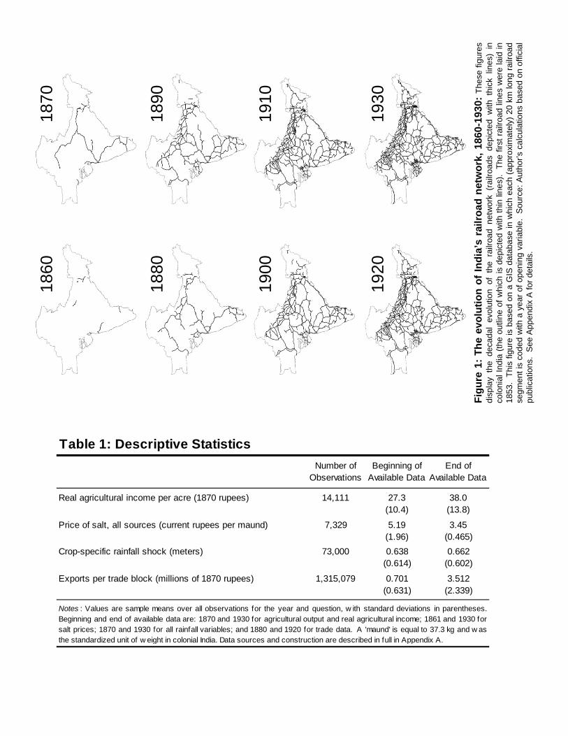
0000 The

sefig

ures

hic

klin

es)

ins

wer

ela

idin

lon

gra

ilroa

dse

do

nof

ficia

l

1930

1910

1890

1870

etw

ork

,18

60-1

930:

Tai

lroad

sd

epic

ted

with

ths)

.T

hefir

stra

ilroa

dlin

es

ch(a

ppro

xim

atel

y)20

kmA

utho

r’sca

lcul

atio

nsb

a s

860

880

900

920

fIn

dia

’sra

ilro

adn

eth

era

ilro

adne

two

rk(r

ais

depi

cte

dw

ithth

inlin

eIS

data

base

inw

hic

hea

cpe

ning

vari

able

.S

ourc

e:de

tails

.

18 18 19 19

1:T

he

evo

luti

on

of

hed

eca

dal

evol

utio

nof

ndia

(the

outli

neof

whi

chis

figur

eis

bas

edo

na

Gis

cod

edw

itha

year

ofop

ns.

See

App

endi

xA

for

d

Fig

ure

disp

lay

thco

loni

alIn

1853

.T

hse

gmen

ti

publ

icat

io

Table 1: Descriptive Statistics

Real agricultural income per acre (1870 rupees) 14,111 27.3 38.0(10.4) (13.8)

Price of salt, all sources (current rupees per maund) 7,329 5.19 3.45(1.96) (0.465)

Crop-specific rainfall shock (meters) 73 000 0 638 0 662

Number of Observations

Beginning of Available Data

End of Available Data

Crop-specific rainfall shock (meters) 73,000 0.638 0.662(0.614) (0.602)

Exports per trade block (millions of 1870 rupees) 1,315,079 0.701 3.512(0.631) (2.339)

Notes : Values are sample means over all observations for the year and question, w ith standard deviations in parentheses.Beginning and end of available data are: 1870 and 1930 for agricultural output and real agricultural income; 1861 and 1930 forsalt prices; 1870 and 1930 for all rainfall variables; and 1880 and 1920 for trade data. A 'maund' is equal to 37.3 kg and w asthe standardized unit of w eight in colonial India. Data sources and construction are described in full in Appendix A. g pp

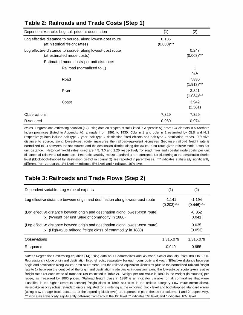
Table 2: Railroads and Trade Costs (Step 1)

Dependent variable: Log salt price at destination (1) (2)

Log effective distance to source along lowest-cost route 0 135Log effective distance to source, along lowest-cost route 0.135(at historical freight rates) (0.038)***

Log effective distance to source, along lowest-cost route 0.247(at estimated mode costs) (0.063)***

Estimated mode costs per unit distance:

Railroad (normalized to 1) 1N/A

Road 7 880Road 7.880(1.913)***

River 3.821(1.034)***

Coast 3.942(2.581)

Observations 7,329 7,329

R-squared 0.960 0.974

Notes : Regressions estimating equation (12) using data on 8 types of salt (listed in Appendix A), from 124 districts in 5 NorthernIndian provinces (listed in Appendix A), annually from 1861 to 1930. Column 1 and column 2 estimated by OLS and NLSrespectively; both include salt type x year, salt type x destination fixed effects and salt type x destination trends. 'Effectivedistance to source, along low est-cost route' measures the railroad-equivalent kilometres (because railroad freight rate isnormalized to 1) betw een the salt source and the destination district, along the low est-cost route given relative mode costs perunit distance. 'Historical freight rates' used are 4.5, 3.0 and 2.25 respectively for road, river and coastal mode costs per unitdistance, all relative to rail transport. Heteroskedasticity-robust standard errors corrected for clustering at the destination district

Table 3: Railroads and Trade Flows (Step 2)

Dependent variable: Log value of exports (1) (2)

level (block-bootstrapped by destination district in column 2) are reported in parentheses. *** indicates statistically signif icantlydifferent from zero at the 1% level; ** indicates 5% level; and * indicates 10% level.

Log effective distance beween origin and destination along lowest-cost route -1.141 -1.194(0.203)*** (0.446)***

(Log effective distance beween origin and destination along lowest-cost route) -0.052x (Weight per unit value of commodity in 1880) (0.041)

(Log effective distance beween origin and destination along lowest-cost route) 0.035x (High-value railroad freight class of commodity in 1880) (0.053)

Observations 1,315,079 1,315,079

R-squared 0.949 0.955

Notes : Regressions estimating equation (14) using data on 17 commodities and 45 trade blocks annually from 1880 to 1920.Regressions include origin and destination fixed effects, separately for each commodity and year. 'Effective distance betw eenorigin and destination along low est-cost route' measures the railroad-equivalent kilometres (due to the normalized railroad freightrate to 1) betw een the centroid of the origin and destination trade blocks in question, along the low est-cost route given relativefreight rates for each mode of transport (as estimated in Table 2). 'Weight per unit value in 1880' is the w eight (in maunds) perg p ( ) g p g ( ) prupee, as measured by 1880 prices. 'Railroad freight class in 1880' is an indicator variable for all commodities that w ereclassif ied in the higher (more expensive) freight class in 1880; salt w as in the omitted category (low -value commodities).Heteroskedasticity robust standard errors adjusted for clustering at the exporting block level and bootstrapped standard errors(using a tw o-stage block bootstrap at the exporting block level) are reported in parentheses for columns 1 and 2 respectively.*** indicates statistically signif icantly different from zero at the 1% level; ** indicates 5% level; and * indicates 10% level.

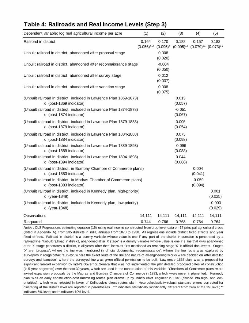
Table 4: Railroads and Real Income Levels (Step 3)

Dependent variable: log real agricultural income per acre (1) (2) (3) (4) (5)

R il d i di t i t 0 164 0 170 0 188 0 157 0 182Railroad in district 0.164 0.170 0.188 0.157 0.182(0.056)*** (0.095)* (0.095)** (0.079)** (0.073)**

Unbuilt railroad in district, abandoned after proposal stage 0.008(0.020)

Unbuilt railroad in district, abandoned after reconnaissance stage -0.004(0.050)

Unbuilt railroad in district, abandoned after survey stage 0.012(0 037)(0.037)

Unbuilt railroad in district, abandoned after sanction stage 0.008(0.075)

(Unbuilt railroad in district, included in Lawrence Plan 1869-1873) 0.013x (post-1869 indicator) (0.057)

(Unbuilt railroad in district, included in Lawrence Plan 1874-1878) -0.051x (post-1874 indicator) (0.067)

(Unbuilt railroad in district included in Lawrence Plan 1879 1883) 0 005(Unbuilt railroad in district, included in Lawrence Plan 1879-1883) 0.005x (post-1879 indicator) (0.054)

(Unbuilt railroad in district, included in Lawrence Plan 1884-1888) 0.073x (post-1884 indicator) (0.098)

(Unbuilt railroad in district, included in Lawrence Plan 1889-1893) -0.096x (post-1889 indicator) (0.088)

(Unbuilt railroad in district, included in Lawrence Plan 1894-1898) 0.044x (post 1894 indicator) (0 066)x (post-1894 indicator) (0.066)

(Unbuilt railroad in district, in Bombay Chamber of Commerce plans) 0.004x (post-1883 indicator) (0.041)

(Unbuilt railroad in district, in Madras Chamber of Commerce plans) -0.059x (post-1883 indicator) (0.094)

(Unbuilt railroad in district, included in Kennedy plan, high-priority) 0.001x (year-1848) (0.025)

(U b ilt il d i di t i t i l d d i K d l l i it ) 0 003(Unbuilt railroad in district, included in Kennedy plan, low-priority) -0.003x (year-1848) (0.029)

Observations 14,111 14,111 14,111 14,111 14,111

R-squared 0.744 0.766 0.768 0.764 0.764

Notes : OLS Regressions estimating equation (16) using real income constructed from crop-level data on 17 principal agricultural crops(listed in Appendix A), from 235 districts in India, annualy from 1870 to 1930. All regressions include district f ixed effects and yearfixed effects. 'Railroad in district' is a dummy variable w hose value is one if any part of the district in question is penetrated by arailroad line. 'Unbuilt railroad in district, abandoned after X stage' is a dummy variable w hose value is one if a line that w as abandonedrailroad line. Unbuilt railroad in district, abandoned after X stage is a dummy variable w hose value is one if a line that w as abandonedafter 'X' stage penetrates a district, in all years after then line w as first mentioned as reaching stage 'X' in off icial documents. Stages'X' are: 'proposal', w here the line w as mentioned in off icial documents; 'reconnaissance', w here the line route w as explored bysurveyors in rough detail; 'survey', w here the exact route of the line and nature of all engineering w orks w ere decided on after detailedsurvey; and 'sanction', w here the surveyed line w as given off icial permission to be built. 'Law rence 1868 plan' w as a proposal forsignif icant railroad expansion by India's Governor General that w as not implemented; the plan detailed proposed dates of construction(in 5-year segments) over the next 30 years, w hich are used in the construction of this variable. 'Chambers of Commerce plans' w ereinvited expansion proposals by the Madras and Bombay Chambers of Commerce in 1883, w hich w ere never implemented. 'Kennedyplan' w as an early construction-cost minimizing routes plan draw n up by India's chief engineer in 1848 (divided into high- and low -priorities) w hich w as rejected in favor of Dalhousie's direct routes plan Heteroskedasticity robust standard errors corrected forpriorities), w hich w as rejected in favor of Dalhousie s direct routes plan. Heteroskedasticity-robust standard errors corrected forclustering at the district level are reported in parentheses. *** indicates statistically signif icantly different from zero at the 1% level; **indicates 5% level; and * indicates 10% level.

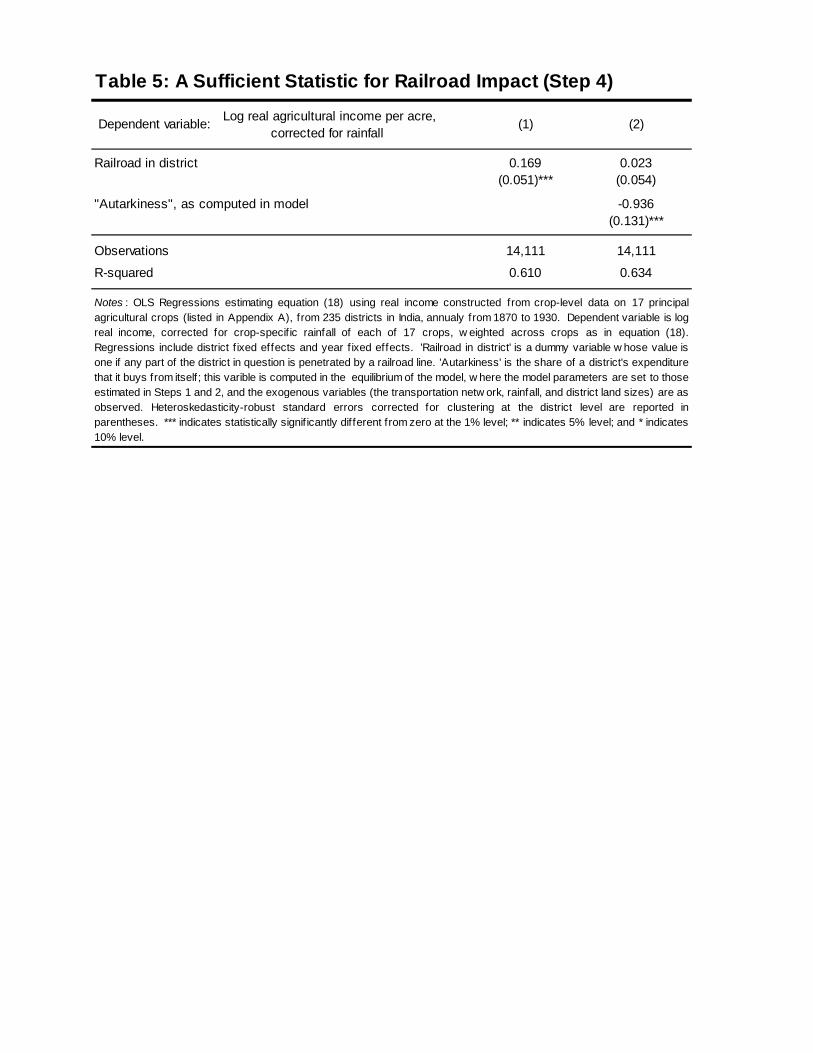
Table 5: A Sufficient Statistic for Railroad Impact (Step 4)

Log real agricultural income per acre,corrected for rainfall

Dependent variable: (1) (2) corrected for rainfall

Railroad in district 0.169 0.023(0.051)*** (0.054)

"Autarkiness", as computed in model -0.936(0.131)***

Observations 14,111 14,111

R-squared 0.610 0.634

Notes : OLS Regressions estimating equation (18) using real income constructed from crop-level data on 17 principalagricultural crops (listed in Appendix A), from 235 districts in India, annualy from 1870 to 1930. Dependent variable is logreal income, corrected for crop-specif ic rainfall of each of 17 crops, w eighted across crops as in equation (18).Regressions include district f ixed effects and year fixed effects. 'Railroad in district' is a dummy variable w hose value isone if any part of the district in question is penetrated by a railroad line. 'Autarkiness' is the share of a district's expenditurethat it buys from itself; this varible is computed in the equilibrium of the model, w here the model parameters are set to thoseestimated in Steps 1 and 2 and the exogenous variables (the transportation netw ork rainfall and district land sizes) are asestimated in Steps 1 and 2, and the exogenous variables (the transportation netw ork, rainfall, and district land sizes) are asobserved. Heteroskedasticity-robust standard errors corrected for clustering at the district level are reported inparentheses. *** indicates statistically signif icantly different from zero at the 1% level; ** indicates 5% level; and * indicates10% level.

A Data Appendix (Not for Publication)

This appendix provides information (supplementary to that in Section 2) on the data used

in this paper.

Sample of Districts:

The data cover the areas of modern-day India, Pakistan and Bangladesh, most of the area

known as British India. I work with a panel of 235 geographic units of analysis that I refer

to as districts, for as much of the period 1870 to 1930 as possible.1

Trade Cost Proxy Variables:

I construct trade cost proxy variables using a newly constructed GIS database on the Indian

transportation network, from 1851 to 1930. The database covers four modes of transporta-

tion: railroads, roads, rivers and coastal shipping. To construct this database, I begin with a

GIS database that contains the locations of contemporary railroad, river and coast lines from

the Digital Chart of the World. Each segment (approximately 20 km long) of the railroad

network is coded according to the year in which it was opened.2 For river transport I keep

only those rivers that are reported in Schwartzberg (1978) or Bourne (1849) as navigable in

1857. The final component of the colonial India GIS database that I construct is the location

of each district and salt source. To calculate district locations I digitize a map of the district

borders in India (as they existed in 1891) based on maps in the Indian Administrative Atlas

and Constable’s Hand Atlas of India (Bartholomew, 1893). I use this to calculate district

centroids, which I take to be the ‘location’ of each district. Finally, I obtain the location of

each salt source from contemporary maps.

I then convert the GIS database of transportation lines and district/salt source locations

into a graph of nodes and arcs, as is common in the transportation literature (Black, 2003).

1The majority of British India was under direct British control, and was divided into nine large, admin-istrative units known as provinces. Each province was further sub-divided into a total of 223 districts, but4 of these districts represent the four major port cities of colonial India (Bombay, Calcutta, Karachi andMadras) which do not report agricultural output consistently and I therefore leave these city-districts outof my sample (see Appendix C, however). Areas not under direct British control were known as ‘PrincelyStates’. For administrative purposes these were grouped into divisions similar to the provinces and districtsdescribed above, so in princely state areas I use the lower administrative units as my units of analysis andrefer to them as districts, following the Indian Administrative Atlas (Singh and Banthia, 2004). There were251 of these districts in my sample area, but data collection in the princely states was extremely incompleteand I include only 16 districts from the princely state regions in my final sample. In sum, I track 219agricultural districts of British districts plus 16 princely state districts annually from 1870-1930.

2To do this I use the publication History of Indian Railways, Constructed and in Progress (1918 and1966 volumes), the 1966 volume of which refers to railroad lines in modern-day India only. To obtain yearsof opening for line segments in modern-day Pakistan and Bangladesh from 1919 to 1930 I use the annualRailway Reports published by the Railways Department, which list all line section openings in each year.

1

I work with a simplified graph representation of the Indian transportation network, where

the number of nodes and the sparsity of arcs is low enough for network algorithms to be

feasibly operated on it using a desktop computer (the resulting network has 7651 nodes).

To do this, I use the ‘simplify’ command in ArcGIS. A line in ArcGIS is a series of vertices

connected by straight lines. The ‘simplify’ command removes vertices in such a way as to

minimize the sum of squared distances between the original line and the simplified line. The

original Digital Chart of the World railroad layer, for example, consists of approximately

33,000 vertices; I simplify the railroad layer to one of only 5616 vertices.

Because the density of informal roads was extremely high (Deloche, 1994), I allow road

transport to occur along the straight line between any two nodes on the network, but only if

the two nodes either represent districts or salt sources, or the two nodes are within 1000 km

of each other.3 The result is a network with 7651 nodes, 5616 of which represent the railroad

network, 660 of which represent the navigable river network, 890 of which represent coastal

shipping routes, 477 of which represent the centroids of the 477 districts in India (in 1891

borders), and 8 of which represent the locations of the sources of 8 different types of salt.

Because the railroad arcs are coded with a year of opening indicator, this network can be

restricted to represent the transportation network for any year from 1851 to 1930 by simply

turning these arcs on or off.

Finally, I use this network representation of the Indian transportation system to calculate

the variable LCRED(α,Rt), described in Section 4. This variable is a measure of the cost

of traveling between any two points (where a point is either a district or a salt source) in a

year using the lowest-cost route along the network (available in that year). The lowest-cost

route depends on the value of the relative per unit distance costs of using each mode (rail,

river, coast, or road), α, and the available transportation network, Rt, whose construction

was described above. Conditional on values of α, I use a standard algorithm from graph

theory and transportation science (Dijkstra’s algorithm, implemented using the Boost Graph

Library for Matlab) to calculate the shortest path between every pair of points, along the

transportation network available in each year from 1870 to 1930. The resulting measure,

LCREDodt(α,Rt), is in units of railroad-equivalent kilometers due to the normalization of

αrail = 1.

Bilateral Trade Flows:

3Allowing straight-line road travel between any two nodes would yield a network with over 58 millionarcs. The shortest path between each of the nodes on such a dense network cannot be calculated using adesktop computer, so I restrict many of these arcs to be non-existent; the result is that the 7651-by-7651matrix representing the network can be stored as a sparse matrix, and analyzed using sparse matrix routines(that increase computation speed dramatically) in Matlab.

2

The data I use on bilateral trade flows was collected from a variety of different sources, one

for each mode of transportation. I describe here each of these modes in turn, and then how

they were combined into aggregate data on trade flows.

Data on railroad trade within India were published separately for each province. The

geographic unit of analysis in these records is the ‘trade block’, which spans between four and

five districts.4 Four of these trade blocks represented the four major ports of colonial India

(Bombay, Calcutta, Karachi and Madras). When a port was represented in this publication

its imports included the sum of imports from other regions of India destined for export

out of the port city by sea (for either international export or export by coasting trade to

another port within India), or destined for consumption/absorption within the port city;

an analogous situation held for exports. After subtracting trade destined for coast-wise

trade (using the coasting trade data described below) I therefore treat these four port city

trade blocks as four economic units whose trade demands and supplies represent the sum of

both intra-city and international demands and supplies for and of goods. (This treatment

is described in detail in Appendix C below.) The railroad trade flow data, like that on all

modes of transportation described below, represents final shipments between two regions

(even if a shipment changed railroad companies).5 Only if a shipment was taken off the

railroad system and re-shipped onwards would it be counted as two separate shipments. I

collect this data from various annual, provincial publications from 1880 onwards.6

Data on river-borne trade within India were published in a similar manner to (and often

along side) the railroad trade data, for the Brahmaputra, Ganges and Indus river systems.

I collect the river-borne trade data from the railroad trade statistics publications for the

riverine provinces of Assam, Bengal, Northwestern Provinces, and Sind, and follow similar

procedures to those described for the rail data above.

Data on trade within India that occurred via coastal shipping were published by each of

the coastal provinces (Bengal, Bombay, Madras and Sind) in a similar manner to the railroad

4Trade blocks split into smaller blocks over time, but I aggregate over these splits to maintain constantgeographic units. The trade blocks were always drawn so as to include whole numbers of districts.

5All bilateral block-to-block intra-provincial trade flows were published, except that from a block to itself(which was always unreported). Inter-provincial trade flows were published from each internal block to eachexternal province (and vice versa), but not by trade block within the external province. I therefore create afull set of inter-provincial block-to-block flows by assigning a province’s trade block’s imports from each ofanother province’s trade blocks in proportion to the exporting blocks’ stated exports to the entire importingprovince (and vice versa for exports).

6The titles of these publications changed over time, from Returns of the Rail [and River-borne] Tradeof [Province] to Report on the trade carried by rail [and river] in [Province] to Report on Inland Trade of[Province]. In the province of Madras, these statistics were only published from 1909 onwards. Railroadtrade statistics were not published by the princely states themselves, but each province’s external tradeto/from each of the large princely states were published. I therefore treat each large princely state (CentralIndia Agency, Hyderabad, Mysore, Rajputana and Travancore) as a single trade block.

3

trade data. I collect the coastal trade data from various annual, provincial publications.7

Trade data by all modes of transport discussed above were published disaggregated by

commodities. In order to compare commodities across these different levels of aggregation,

I aggregate all data to the level of the 17 commodities (listed below) for which agricultural

output and price data are available. Finally, I aggregate the trade data on each of the modes

(for each commodity separately) into one trade dataset. All of the above trade data are

available from at least 1865 onwards, except for the railroad and river trade data which

starts in a coherent manner in 1880 and was discontinued in 1920. I therefore use bilateral

trade data from 1880 to 1920 only. This generates the variable Xkodt in the text.

Rainfall Data:

A thick network of 3614 rain gauges at meteorological stations scattered throughout colo-

nial India recorded daily rainfall amounts from 1891-1930. From 1901 onwards, these records

have been digitized by the Global Historical Climatology Network (Daily) project; the GHCN

dataset also provides the latitude and longitude of each station. For the years 1891-1900, I

collect the data from the publication, Daily Rainfall for India in the year.... In the years 1870

to 1890, very little daily rainfall data were published in colonial India, but monthly data from

365 stations (spread throughout India) were published by each province.8 I convert monthly

station-level data to daily station-level data using a modeling procedure that is common in

the meteorological statistics literature (eg, Ngo-Duc, Polcher, and Laval (2005)).9 I convert

station-level data to district-level data by simply averaging over the many stations in each

district.10 Finally, as described in Section 5, I use the Indian Crop Calendar (Directorate of

Economics and Statistics, 1967) to compute the total amount of rain that fell during each

crop’s growing season (as defined in the Crop Calendar), in each district and year.11 This

7The coastal trade data were published in publications whose titles changed from Annual Statement ofthe Sea-borne Trade and Navigation of [Province] to Report on the Maritime Trade of [Province].

8These publications included the Administration Reports for each province, described in the agriculturalprice data section below. I use additional data (to increase the number of stations) that were published inselected provinces’ Sanitary Reports.

9Specifically, using daily data from 1891 to 1930, I estimate the district-specific relationship between thepattern of monthly rainfall in a year and the rainfall on any day of that year; I then use these estimatedrelationships to predict the rainfall on any day in a given district and year from 1870 to 1890, conditionalon the pattern of monthly rainfall actually observed in that district and year. While these daily rainfallpredictions are likely to be imprecise, much of the imprecision is averaged over when I construct crop-specific rainfall shocks, which are measures of the total rainfall in a given period (a length ranging from 55to 123 days.)

10If a given district-day has no reported rainfall observations I impute this missing observation by using aninverse distance-weighted average of that day’s rainfall in the 5 closest reporting stations (know as “Shepard’smethod” in the meteorological literature (Shepard, 1968)).

11This crop calendar covers the regions of colonial India that are in modern-day India, but not Bangladeshor Pakistan. For districts in Bangladesh and Pakistan I assign growing seasons (to each crop) that reflect

4

generates the variable RAINkot used in the text.

Prices of Salt and Agricultural Commodities:

I use data on eight different types of salt12 for each of the six provinces in Northern India

as well as data on 17 agricultural commodities13 from all of India. I collect this price data

from various annual, provincial publications.14 Prices reported in these publication were an

average of observations taken by district officers once per fortnight at each of 10-15 leading

retail markets per district.

Real Agricultural Income:

I use data that present the area under each of 17 crops (the 17 for which price data are

available), and the yield per acre for each of these crops, in each district and year.15 I take

the product of each area and yield pair to create a measure of real output for each crop,

district and year. I then evaluate this bundle of 17 real output measures at the retail prices

prevailing for these crops (from the agricultural price data described above), in each district

and year, to create a measure of total nominal agricultural output for each district and year.

Finally, I divide nominal output by a consumer price index (the Tornqvist index) to create

a measure of real income.16

an average of the start and end dates (of the reported growing season) in the five nearest Indian districts.12These eight salt types are those from: the Bombay sea salt sources near the city of Bombay, salt from

the UK distributed via Calcutta, the Didwana salt source in Punjab, the Kohat mines in Punjab (principallythe Jatta mine, according to Watt (1889)), the Mandi mine in Punjab, the Salt Range mines in Punjab(principally the Mayo mine, according to Watt (1889)), the Sambhar Salt Lake in Rajputana, and theSultanpur source in the Central India Agency.

13These crops are: bajra, barley, bengal gram, cotton, indigo, jowar, kangni, linseed, maize, opium, ragi,rape and mustard seed, rice, sesamum, sugarcane, tur and wheat.

14These publications are: Prices and Wages in India; Administration Reports from all provinces; theSalt Report of Northern India; the Statistical Atlas of Andhra State with agricultural price data (for theMadras Presidency); the Season and Crop Reports from various provinces with agricultural price data; andthe Sanitary Reports from various provinces with data on prices of food grains.

15These data were published in Agricultural Statistics of India from 1884 to 1930. For the years 1870-1883I use data on crop areas and yields in the provincial Administration Reports, as described in the agriculturalprices data section above. Data on agricultural output were published in each province’s AdministrationReport except for Punjab and Bengal. For supplementary data I use each province’s Season and CropsReport between 1904 and 1930. While Blyn (1966), Heston (1973), and Dewey (1979) have discussed thepotential for measurement error in these sources, these authors have not been concerned with mechanismsthrough which measurement error might be correlated (conditional on the fixed effects in place) with theregressors I use in this paper.

16In order to compute this consumer price index I use district and year specific consumption weights,computing consumption as output minus net exports (assigning net exports, within each commodity, pro-portionally across districts within each trade block).

5

B Proof of Prediction 3 (Not for Publication)

Consider the simplified version of the model, as in Section 3.2 (the simplified version of which

was only assumed to obtain Prediction 3). That is, there are only three regions o (X, Y and

Z), one commodity, and the regions are initially symmetric (Lo = 1, Ao = Aλθ1, Tod = T

for all o 6= d, and Tod = 1 for all o = d). Now consider a symmetric change in trade costs

between regions X and Y only (ie dTXY = dTY X 6= 0) and solve for the change in region

X’s real income (dWX = drX − dpX). Let rX = 1 at all times (ie drX = 0) by choice of the

numeraire; by symmetry the same holds true for rY . Solving for the change in real income

is then simply a matter of solving for dpX , since dWX = −dpX .

Totally differentiating the price equation for pX (equation (4)) and evaluating this around

the symmetric initial equilibrium we obtain

p−(θ+1)dpX = AT−(θ+1)dTY X + AT−θdrZ , (1)

where po = p = A−1/θ(1 + 2T−θ)−1/θ. To obtain an expression for drZ , totally differentiate

region Z’s land market clearing condition (equation (6)) around the symmetric equilibrium

to obtain

[(1 + θ)A−1 − pθZ ]drZ = 2θpθ−1T−θdpX + θpθ−1dpZ , (2)

where this step uses the fact that, because of symmetry, dpX = dpY . Finally, note from

the price equation for region Z (ie equation (4)), total differentiation around the symmetric

equilibrium again implies

dpZ = Apθ+1drZ . (3)

Substituting equations (2) and (3) into equation (1) we obtain[1− 2θT−2θ

(1 + θ)A−2p−2θ − θ − A−1p−θ

]dpX = pθ+1AT−(θ+1)dTXY . (4)

Noting that A−1p−θ = (1 + 2T−θ), this simplifies to[1− 2θT−2θ

4(1 + θ)T−2θ + (4θ + 2)T−θ

]dpX = pθ+1AT−(θ+1)dTXY . (5)

Since the expression in square brackets is positive (for θ > 0, as maintained throughout the

paper) the change in region X’s prices (dpX) is of the same sign as the change in trade costs

(dTXY = dTY X). That is, real income in region X rises as trade costs between region X and

another region (here, region Y ) fall, which is Prediction 3. This concludes the proof.

6

C Including Port Cities (Not for Publication)

The four main port cities of colonial India (Bombay, Calcutta, Karachi and Madras) present

a number of circumstances that require them to be handled differently from other regions of

India. I describe here how these cities entered my analysis, section by section.

Section 4:

The 124 districts of Northern India that are included in my analysis of salt price data include

the two relevant Northern port cities of Karachi and Calcutta.

Section 5:

The 45 trade blocks included in my analysis of bilateral trade patterns include 4 blocks

that refer to the four main port cities. These blocks included, as described above, trade

data reporting each Indian region’s total trade with the given port city with no distinction

between whether that trade was with inhabitants of the city or with the wider world via

the particular port in question. Because of this, the four trade blocks should be interpreted

as representing the composite economic activity of two sub-economies: (i) the port city in

question, and (ii) the segments of the rest of the world that choose to trade with India via

the port in question. This decision has no bearing on the estimation of θk in equation (14)

due to the inclusion of importer and exporter fixed effects (separately for each commodity

and year). However, when estimating κ in equation (15) the four port city blocks are not

included. This is because I lack data on rot (nominal agricultural output per acre) for cases

in which o is a port city block, so I cannot equate the estimate, ln βkot + θ ln rot, to lnAkot.

Further, I do not observe the appropriate international equivalent of RAINkot required to

estimate equation (15) for these port city blocks. (Note that even if equivalent international

data on rainfall by crop were available, using this data would require me to take a stand on

the trade costs that separate each port city block from each country in the world. Estimating

these international trade costs would be challenging due to the absence of internationally

comparable price data like that used in Section 4. By contrast, the strategy I employ here

does not require data on these international trade costs.)

Section 6:

As discussed above, while the four port cities were each contained in eponymous districts of

British India, I do not include these four districts in my panel of 235 districts that are used

in the regressions in Sections 6 and 7. The reason for this is that my analysis is focused

on the determinants of real agricultural income, and these four port cities did not report

7

agricultural output data (because so little agriculture was taking place in these city-districts).

Section 7:

A final challenge presented by the four port cities (which, recall, are treated as a composite of

domestic and international economic regions) is that their demand for and supply of goods is

likely to have had important effects on the 235 non-port Indian districts in whom my interest

lies, and these effects will have changed as interior districts became connected by railroads

to the port cities and thence the wider world. For this reason, I compute the equilibrium to

the model with 239 separate regions: 235 Indian districts plus four port cities (which include

the rest of the world). Doing this requires data on the key exogenous variables—the effective

productivities (Akot) and land areas (Lo)—from the four port city regions, but such data are

unavailable. These exogenous variables are required to compute equation (6) (which depends

explicitly on Lo and implicitly, through the definition of πkod, on Ako). To circumvent this

data shortage I use the structure of the model to proceed as follows. To begin, note that

the estimates of eβkot obtained (in Section 5) for the port city regions are equal to Akotr

−θkot .

Since Akot appears in equation (6) only when multiplied by r−θkot I substitute the estimates of

eβkot (for the four port city blocks only) from Section 5 into equation (6). After this substitu-

tion has been made, the system of equations defined by equation (6) contains the unknown

endogenous variable ro for cases in which o is a port city region only when ro is multiplied

by Lo (which, for port city regions, is also unknown due to lack of data on land areas). I

therefore simply solve for the composite roLo (but only for the regions o referring to port

city regions) that satisfies the system of equations defined by equation (6).

8

Appendix References (Not for Publication)

Bartholomew, J. G. (1893): Constable’s Hand Atlas of India. London: A. Constable.

Black, W. R. (2003): Transportation: A Geographical Analysis. Guilford: The Guilford

Press.

Blyn, G. (1966): Agricultural Trends in India, 1891-1947: Output, Availability, and Pro-

ductivity. Philadelphia: University of Pennsylvania Press.

Bourne, J. (1849): Indian River Navigation. London: W. H. Allen.

Deloche, J. (1994): Transport and Communications in India Prior to Steam Locomotion:

Volume I: Land Transport. Oxford: Oxford University Press.

Dewey, C. (1979): “Patwari and Chaukidar: Subordinate Officials and the Reliability of

India’s Agricultural Statistics,” in The Imperial Impact in Africa and South Asia, ed. by

C. Dewey, and A. Hopkins. London.

Directorate of Economics and Statistics (1967): Indian Crop Calendar. Delhi:

Government of India Press.

Heston, A. (1973): “Official Yields per Acre in India, 1886-1947: Some Questions of

Interpretation,” Indian Economic and Social History Review, 10(40), 303–334.

Ngo-Duc, T., J. Polcher, and K. Laval (2005): “A 53-year Forcing Data Set for Land

Surface Models,” Journal of Geophysical Research, 110, 1–13.

Schwartzberg, J. E. (1978): A Historical Atlas of South Asia. Chicago: University of

Chicago Press.

Shepard, D. (1968): “A Two-Dimentional Interpolation Function for Irregularly-Spaced

Data,” Proceedings of the National Conference, ACM, 23, 517–524.

Singh, R., and J. Banthia (2004): India administrative atlas, 1872-2001. New Delhi:

Conroller of Publications.

Watt, G. (1889): A dictionary of the products of India. London: J. Murray.

9